Download Solution 2.0 SOLUTION TLB GROUP User`s Manual

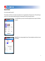
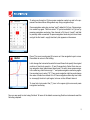
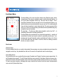
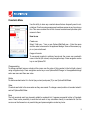
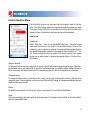
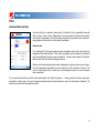
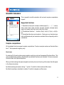
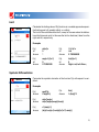
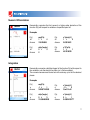
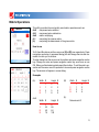
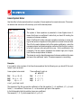
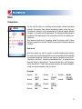
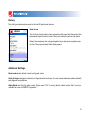
Solution 2.0
SOLUTION TLB GROUP
User’s Manual
Table of Contents
Introduction
3
Quick Start 4
User’s Interface
- Main Menu
- Help
- Functions Menu
- Constants Menu
- Custom Functions Menu
6
Plot
- General description
- Navigation
- More Functions Menu
12
Scientific Calculator
- Supported functions
- Complex computations
14
Analysis
- Limit
- Symbolic Differentiation
- Numeric Differentiation
- Integration
15
Matrix Operations
18
Solvers
- Non-linear Equation solver
- Linear-System Solver
- ODE Solver
19
More
- Conversions
- History
- Settings
22
Credits
24
End-User License Agreement
25
Disclaimer
26
Introduction
Solution is the most powerful mathematical application for mobile devices running Symbian OS Nokia
Series 60 3rd Edition. Solution contains lots of different instruments and provides smart interface which
makes using Solution quick and easy.
This document describes all the Solution features and abilities and the right way to use them.
In the 2nd chapter – Quick Start – you can find a detailed description of plotting exp(x) function. This simple
example will introduce the basic interface features.
In the 3rd chapter – User’s Interface – the interface utilities that are used in the whole program are widely
discussed. The main idea of Solution interface is in fact this simply one – to enter any data press navigation
centre key first and look at the appeared dialog if any.
In the 4th – 8th chapters you can find full description and detailed how-to-use instructions for all the Solution instruments such as Plot, Calculate, Analysis, Matrix and Solve.
In the 9th chapter – More – you can find descriptions of some more utilities and settings that can be used
in Solution.
We hope that you would find Solution useful and worthwhile application.
Good luck!
Quick Start
How to plot exp(x) function?
The interface of Solution is simple and provides a lot of opportunities at the same time. The best thing is
just to try it on the simple example and get the main ideas. So let’s plot exp(x) function!
In the Main Menu you see six icons that represent six main parts of Solution
program.
Select Plot icon using navigation keys. Press navigation centre key to open
Plot dialog.
To enter new formula in F(x) box press navigation centre key and in the appeared Functions Menu dialog select exp using navigation keys.
Press navigation centre key and see “exp()” added to F(x) box. Press navigation centre key again. This time select “x” symbol and add it to F(x) box by
pressing navigation centre key. Now formula in F(x) box is “exp(x)” and that
is precisely what we wanted. So press navigation centre key two more times
and get the first result – exp(x)-function’s plot appears on the screen.
Press [*] to zoom in and press [#] to zoom out. Use navigation keys to move.
Press back to return to Plot dialog.
Let’s change the horizontal bounds Xmin and Xmax that specify the original
position of function’s graph to -10 and 2 respectively. Select Xmin box using navigation keys (press down three times). To enter minus press navigation centre key, select minus sign “-” and press navigation centre key again.
Use number keys to enter “10”. Then press navigation right key and change
the value of Xmax from default 5 to 2. Press navigation centre key two times
to view exp(x)-function’s plot again, but now on the different interval.
To view help topic select the [?] icon in the upper-right corner and press
navigation centre key.
Now you are ready to start using Solution! To learn all the details concerning Solution instruments read the
following chapters.
User’s Interface
Main Menu
In the Main Menu you see six icons that represent six main parts of Solution
program.
The first item is Plot – using this utility you can plot any functions quickly
and easily. You can view several graphs on the same worksheet or vary
functions using parametric dependencies.
The second item is Calculate – you can evaluate any expression using this
scientific calculator that supports even complex computations. You may
create your own functions and remember frequently used constants and
then refer to them by name.
The third item is Analysis – it includes several powerful mathematical instruments concerning function analysis. Solution can evaluate limiting values,
numerically integrate and differentiate functions and even find out symbolic
derivatives.
The next item is Matrix – this utility includes widely-used matrix operations.
The next item is Solve – this instrument will help you to solve non-linear
equations, linear systems or ordinary differential equations quickly using
numerical methods with high accuracy in calculations.
The last item is More – there are several utilities and settings that could be
used in Solution.
Help
There is a help topic for each instrument of Solution program.
Help is available in any dialog. To view help topic for an instrument (plot, calculate etc) open the necessary utility and select [?] icon if it’s available and
press navigation centre key. In some menus (e.g. Functions Menu) there is
no such icon. In this case use Options/Help to open the related help topic.
Functions Menu
Functions Menu is the main tool that makes using Solution quick, smart,
nice and easy. This menu is available nearly in every instrument dialog – to
call it just press navigation centre key. The main idea is simple – Functions Menu indicates what you are able to do in the particular situation, e.g.
which function you can use and which one you can not. For mobile phones
it’s a well-known problem to enter formulas fast. The main purpose of this
utility is, of course, to make entering formulas as fast as possible using only
navigation keys and numbers.
The principle – “To enter any data press navigation centre key first” – is
something like Solution interface general rule.
Functions Menu also provides the very important opportunity – creation of
user-defined functions and quick access to previously saved ones. If expressions are big and frequently used in calculations it takes a lot of time
to print them each time you need to. So this is time for creating a custom
function or save a constant.
How to use
Standard items
To enter standard function or constant value select the necessary one using navigation keys and press the
navigation centre key. Any standard item that can’t be used in the particular case is marked grey.
User-defined items
You can define your own constant/function using Constants and Custom Functions menus respectively. To
call Constants menu press [*]. To call Custom Functions menu press [#]. Use these utilities to store any constants and functions that are frequently used. Give them unique names and then use them in any formula.
To learn more about creation, changing and using constants and custom functions open the appropriate
menu and call Options/Help there.
Details
Here are brief descriptions of every Functions Menu standard item.
x – independent variable
pi, e – constants.
sin, cos, tan, ctg, asin, acos, atan, actg – trigonometric functions
sh, ch, th, cth – hyperbolic functions
exp - exponent
ln – natural logarithm
log – logarithm of base 10
sqrt – square root of a number
abs – absolute value
i – imaginary unity
re, im – real and imaginary parts of a complex number
+ - ^ * / – arithmetic operations
! – factorial function
Ank = n!/(n-k)! – combinatorial function
Cnk = n!/(k!*(n-k)!) – combinatorial function
(), (, ) – brackets
, – delimiter between arguments in multidimensional user-defined function
A – numeric parameter in plotter
E – scientific notation sign, e.g. 2E3=2*10^3=2000
Ans – the last answer
y – desired function in Cauchy problem.
Constants Menu
Use this utility to store any constant values that are frequently used in calculations. Give them unique names and use these names in any formula you
like. This menu contains the full list of saved constants and provides quick
access to them.
How to use
Create new
Select “Add new…” item or use Options/Edit/Add new… Enter the name
and the value to be saved in the appeared dialogs. Some of the names (e.g.
pi or e) are not allowed.
Usage in formula
To use saved constant in arbitrary formula set the cursor over constant’s
name in the list (left column) using navigation keys. Press navigation centre
key or use Options/OK.
Change existing
To change constant (name or value) set the cursor over the value of this constant in the list (right column)
using navigation keys. Press navigation centre key or use Options/Edit/Change. In the appeared dialogs
enter new name and then new value.
Delete
To delete constant select it in the list (any column) and press [C] or use Options/Edit/Delete.
Order
Constants are listed in the same order as they were saved. To change current position of constant select it
and call Options/Edit/Order.
More
The last numerical result can be easily added to constants list. It appears as special button in Constants
menu. There is also possibility to save the last result of any calculation directly to constants list. Set the
cursor over the Answer box in parent dialog and press navigation centre key twice.
Custom Functions Menu
Use this utility to store any functions that are frequently used in calculations. Give them unique names and use these names anywhere you need.
This menu shows the full list of user-defined functions and provides quick
access to them. User-defined functions can be multidimensional.
How to use
Create new
Select “Add new…” item or use Options/Edit/Add new… Enter the unique
name and the formula to be saved in the appeared dialog. Some of the
names (e.g. sin or exp) are not allowed. To create multidimensional function
use several independent variables – the names of them should be “x1”, “x2”
etc. See the example below for details. The current function from parent
dialog can be easily saved. It appears as special button in Custom Functions menu.
Usage in formula
To use saved function set the cursor over it’s name in the list (left column) using navigation keys. Press navigation centre key or use Options/OK. If function is multidimensional it is added to parent dialog with brackets and commas. You should specify all the necessary arguments. See the example below for details.
Change existing
To change function (name or formula) set the cursor over the it’s formula (right column in the list) using
navigation keys. Press navigation centre key or use Options/Edit/Change. In the appeared dialog enter new
name and then new formula.
Delete
To delete function select it in the list (any column) and press [C] or use Options/Edit/Delete.
Order
Functions are listed in the same order as they were saved. To change current position of function select it
and call Options/Edit/Order.
10
Multidimensional function example
Suppose you want to save the function fun(x1,x2) = sin(x1)+x2. Select “Add new…” item and enter the
function’s name fun. Enter the formula (Functions Menu is available) sin(x1)+x2. Press OK or press centre
key twice.
To use new function select its name and press centre key. In the parent dialog fun(,) appears. The comma
separates arguments. Enter the values for both arguments (that can be numbers, other functions, variables
or expressions) and get the answer. fun(0,1) provides 1, fun(asin(1), -1) provides 0.
11
Plot
General Description
Use this utility to create a linear plot of function F(x) in specified bounds
Xmin, Xmax, Ymin, Ymax. Parameter A can be used in F(x) formula, specify
this value if necessary. This utility also provides an opportunity to view several graphs of functions on the same worksheet.
How to use
For entering F(x) formula quicker press navigation centre key and use the
appeared Functions Menu. This menu provides quick access to standard
and user-defined functions and constants. To learn more about Functions
Menu read User’s Interface chapter above.
When you finish entering data press navigation centre key two more times.
On the appeared worksheet you will see plot of F(x) function. Press [*] to
zoom in and press [#] to zoom out, use navigation keys to move through
the worksheet.
To view several functions on the same worksheet use “More functions…” menu (select this item and press
navigation centre key). You can change existing functions and add new ones to the same worksheet. To
learn more read the information below.
12
More Functions Menu
Use this utility to view several functions’ graphs on the same worksheet.
How to use
Create new
Select “Add new…” item or use Options/Edit/Add new… Enter the function
in the appeared dialog (Functions menu is available).
Change existing
To change the function (name or formula) select it from the list (left column)
using navigation keys. Press navigation centre key or use Options/Edit/
Change. In the appeared dialog make the necessary changes.
To change the color of function’s graph set the cursor over the right column
in the list and press navigation centre key. In the appeared dialog make the
necessary changes.
Delete
To delete function from the list select it (any column) and press [C] or use
Options/Edit/Delete.
Order
Functions are listed in the same order as they were saved. To change current position of function select it and call Options/Edit/Order.
Plot
To plot all the functions use Options/Plot.
13
Scientific Calculator
This is powerful scientific calculator with real and complex computations
support.
Supported functions
1. Standard functions (with complex-variable support): +, – , /, *, ^, sqrt(x),
sin(x), cos(x), tan(x), ctg(x), arcsin(x), arccos(x), arctan(x), arcctg(x) exp(x),
log(x), ln(x), abs(x), re(x), im(x), sh(x), ch(x), th(x), cth(x).
2. Combinatorial calculus: ! – factorial, A(n,k)= n!/(n-k)!, C(n,k) = n!/(k!*(nk)!).
3. User-defined functions and constants – Create your own functions (possibly multidimensional) and remember constants that are frequently used in
calculations.
Complex computations
All the standard functions support complex computations. To enter a complex number use Function Menu
item “i” that represents imaginary unity.
How to use
For entering F(x) formula quicker press navigation centre key and use the appeared Functions Menu. This
menu provides quick access to standard and user-defined functions and constants. To learn more about
Functions Menu call Options/Help there.
When you finish entering data press navigation centre key two more times to get the answer that will appear
in the Answer box below.
By default pressing [#] causes entering “.” symbol. To switch to Alpha mode use More menu.
By default everything is calculated in radians. To switch to degrees use More menu.
14
Analysis
This utility includes several function analysis tools such as: Limit, Symbolic
and Numerical Differentiation and Numerical Integration. The detailed description of each instrument is provided below.
How to use
For entering F(x) formula in each of these instruments quicker press navigation centre key and use the appeared Functions Menu. This menu provides
quick access to standard and user-defined functions and constants. To
learn more about Functions Menu read User’s Interface chapter above.
When you finish entering data press navigation centre key two more times
to get the answer that will appear in the Answer box below.
15
Limit
Calculates the limiting value of F(x) function as x variable approaches specified limiting point x0, possibly infinity, or –infinity.
The limit is the real bidirectional limit, except in the case where the bidirectional limit does not exist. In this case the limit is directional, taken from the
right and left, respectively.
Examples
F(x)
x0
Answer
F(x)
x0
Answer
sin(x)/x
0
1
exp(x+1)/(x+1)
0
2.718281828
F(x)
x0
Answer
F(x)
x0
Answer
(1+1/x)^x
+inf
2.7182804690
ln(x)/(x+1)
0
Right: -inf; Left: Error;
Symbolic Differentiation
Computes the symbolic derivative of the function F(x) with respect to variable x.
Examples
F(x)
Answer
F(x)
Answer
F(x)
Answer
exp(2*x)
2*exp(2*x)
F(x)
Answer
th(x)
1-(th(x))^2
sin(x)*exp(x)
sin(x)*exp(x)+exp(x)*cos(x)
x^(sin(x)+1)
(ln(x)*cos(x)+(1+sin(x))/x)*x^(1+sin(x))
16
Numeric Differentiation
Numerically computes the first, second, or higher–order derivative of the
function F(x) with respect to variable x at specified point x0.
Examples
F(x)
x0
Answer
F(x)
x0
Answer
exp(2*x)
1 k
4
118.224898
F(x)
x0
Answer
x^(sin(x)+1)
1 k
2
2.63014901
sin(x)*exp(x)
0 k
3
2
F(x)
x0
Answer
x^(2*pi*x)
1 k
1
45.7616029
Integration
Numerically computes a definite integral of the function F(x) with respect to
the variable x over the straight line from a to b (finite numbers).
The numerical answers are carried out with accuracy up to the five decimal
places.
Examples
F(x)
a
Answer
F(x)
a
Answer
exp(2*x)
-1 b
1
3.62687166380
sin(x)*exp(x)
0 b
3
11.8594882628
F(x)
a
Answer
F(x)
a
Answer
x^(sin(x)+1)
-1 b
0
Can’t Do It!
x^(sin(x)+1)
0 b
1
0.40824193777
17
Matrix Operations
This utility provides the most widely used matrix operations such as:
A+B
component-wise addition
A-B
component-wise subtraction
AxB
matrix multiplying
A-1
computing the inverse matrix
|A|
computing the determinant of the given matrix
How to use
To fill A and B matrices set the cursor over [A] or [B] icon respectively. Press
navigation centre key. In appeared dialog you can change the size and elements of matrix you’ve chosen.
To enter element set the cursor over its position and press navigation centre
key. Change the value and press navigation centre key once more or use
OK. When you finish entering data press Save button. To call the matrix operation set the cursor over the operation’s icon and press navigation centre
key. The answer will appear in a new dialog.
Examples
(A): Width 3
1
2
3
AxB:
1
1
4
7
Width 2
1
2
3
1
22
49
76
Width 2
Height 3
(B)
2
2
5
8
1
2
3
3
3
6
9
Height 3
|A|:
1
1
3
5
Height 3
2
2
4
6
Determinant: 0
2
28
64
100
18
Solvers
Non-linear Equation solver
Use this utility to find numerical solution to a single equation f(x)=0 solved
for a single unknown x over the straight line from a to b (finite numbers).
The numerical answers are carried out with accuracy up to the five decimal
places.
How to use
For entering F(x) formula quicker press navigation centre key and use the
appeared Functions Menu. This menu provides quick access to standard
and user-defined functions and constants. To learn more about Functions
Menu call Options/Help there.
When you finish entering data press navigation centre key two more times
to get the answer that will appear in the Answer box below.
Examples
F(x)
a
Answer
F(x)
a
Answer
sin(x)*exp(x)
-1 b
1
0
ln(x)+tan(x)
2 b
4
2.418229103088
F(x)
a
Answer
F(x)
a
Answer
x^2–2
0 b
2
1.41421222686
exp(2*x)
-1 b
1
Can’t Do It!
19
Linear-System Solver
Use this utility to find numerical solution to a system of linear equations for several unknowns. The numerical answers are carried out with accuracy up to the five decimal places.
How to use
The system of linear equations is presented in Linear Algebra terms. It
means that there is a coefficients’ matrix that you should fill minding the
sequence of unknown variables.
Select “Coefficients” button and press navigation centre key. In a new dialog set the number of equations in the system to be solved in Amount field.
Then fill in the matrix displayed with all the system coefficients – select the
necessary element and press navigation centre key. Mind that the k–column
is for the k–unknown value only and the n–row – for the coefficients in the
n–equation. The last column represents the constant right part of equations. See the example below for details.
The answer is a vector, where the sequence of unknown variables is the same
as it was in the coefficients’ matrix. The answer appears in a new dialog.
Examples
If you need to solve a system of the three linear equations like the following one you should fill the coefficients’ matrix as shown.
Linear system to be solved:
Then coefficients’ matrix is:
a1 a2 a3 C
Eq1 2x – y + 3z = 9;
Eq2 5x – y – z = 0;
Eq3
–2y + z = 1.
x is a1, y is a2 and z is a3.
Eq1 Eq2 Eq3
2 –1 3 9
5 –1 –1 0
0 –2 1 1
The elements of the first row are the coefficients of the first equation: 2 – x’s coefficient; (–1) – y’s coefficient; 3 – z’s coefficient. The last one – 9 – is the constant right part of the equation.
In the third equation the first variable x has a zero–coefficient.
The answer is (1 ; 2; 3), which means that x=1; y=2; z=3.
20
ODE Solver
Use this utility to solve initial value problems for ordinary differential equations (ODEs). Specified equation dy/dx= f(x,y), where y(x) is scalar function
depending on x, is numerically solved in the specified interval [x1, x2] using
Euler method.
How to use
For entering F(x) formula quicker press navigation centre key and use the
appeared Functions Menu. This menu provides quick access to standard
and user-defined functions and constants. To learn more about Functions
Menu call Options/Help there. Mind the special symbol “y” that represents
the desired unknown function and can be used in equation. When you finish
entering data press navigation centre key two more times to get the answer.
The numerically resolved answer is plotted in a new dialog.
Examples
dy/dx cos(x)
0
x2
6.3
x1
y(x1) 0
sin(x) is plotted
dy/dx 2*y
x1
0
x2
1
y(x1) 1
exp(2*x) is plotted
dy/dx 2*abs(x)
x1
-1
X2
1
y(x1) -1
y=x^2 for x>0 and y=-x^2 else is plotted
21
More
Conversions
You can use this utility for converting values between various numeration
systems. Conversions from decimal numeration system return the positive decimal numbers in a true representation; the whole negative decimal
numbers – in a complement representation. The fractional negative decimal
numbers are not represented in the complement form for not creating contradictions.
Also there are functions for converting values from binary, octal or hexadecimal numeration to decimal. These functions return the positive decimal
numbers.
How to use
Enter the number you want to convert to another notation (press navigation centre key to enter letters) and then use special buttons that represent
six available operations. In the first row there are “decimal to binary form”,
“decimal to octal form”, “decimal to hexadecimal form”. In the second row
there are “binary to decimal form”, “octal to decimal form” and “hexadecimal to decimal form”. Select the necessary operation and press navigation
centre key. Answer appears in the box below.
Examples
Number
Answer
Number
Answer
4.5
10->2
100.1
1000
[10->16]
3e8
Number
Answer
Number
Answer
-1
[10->2]
1111
Number
Answer
abcdef
[16->10]
11259375
11001
[2->10]
25
22
History
This utility provides quick access to the last 30 performed actions.
How to use
The first line of each history item represents utility used and the second line
represents object (function, matrix etc) upon which the action took place.
Select the necessary item using navigation keys and press navigation centre key. The proper already-filled dialog opens.
Additional Settings
Reset colors sets default values to all graph colors.
Units of Angle changes the behavior of trigonometric functions. You can choose between radians (default)
and degrees computations.
Alpha Mode sets the F(x) editor mode. Digits mode “123” is set by default, letters mode “Abc” is recommended for users of QWERTY-keyboard.
23
Credits
Alexander Taboriskiy
Nadezhda Baldina
Sergey Basheleyshvili
Dmitriy Kuznetsov
http://www.math-solution.com
[email protected]
24
End-User License Agreement
Solution is copyright (C) 2005 - 2008 SOLUTION TLB GROUP. All rights reserved.
This license describes the conditions under which you may use version 2.0 of Solution («the program»). If you are unable or unwilling
to accept these conditions in full, then, notwithstanding the conditions in the remainder of this license, you may not use the program
at all.
You are granted a non-exclusive license to use the program on one device at a time. The program may not be rented, leased or
transferred.
Any use of the program which is illegal under international or local law is forbidden by this license. Any such action is the sole responsibility of the person committing the action.
The program is distributed «AS IS» and you assume full responsibility for determining the suitability of the program and for results
obtained.
SOLUTION TLB GROUP makes no warranty that all errors have been or can be eliminated from the program software and, with respect thereto, SOLUTION TLB GROUP shall not be responsible for losses, damages, costs, or expenses of any kind resulting from
using or misusing the program including without limitation, any liability for business expenses, machine downtime, damages experienced by you or any third person as a result of any deficiency, defect, bug, error or malfunction. SOLUTION TLB GROUP shall not be
liable for any indirect, special, incidental, or consequential damages relating to or arising out of the subject matter of this Agreement
or actions taken hereunder.
NO WARRANTY OF ANY KIND IS EXPRESSED OR IMPLIED. YOU USE THE PROGRAM AT YOUR OWN RISK. SOLUTION TLB
GROUP DISCLAIMS ALL WARRANTIES, EITHER EXPRESS OR IMPLIED, INCLUDING THE WARRANTIES OF MERCHANTABILITY
AND FITNESS FOR A PARTICULAR PURPOSE. NOBODY WILL BE LIABLE FOR DATA LOSS, DAMAGES, LOSS OF PROFITS OR ANY
OTHER KIND OF LOSS WHILE USING OR MISUSING THIS SOFTWARE.
You may not distribute, copy, emulate, clone, rent, lease, sell, modify, decompile, disassemble, otherwise reverse engineer, or transfer
the program, or any subset of the program, except as provided for in this agreement. Any such unauthorized use shall result in immediate and automatic termination of this license and may result in criminal or civil prosecution.
All rights not expressly granted here are reserved by SOLUTION TLB GROUP.
SOLUTION TLB GROUP reserves the right to make exceptions to any of these conditions, or alter these conditions, at any time. However, you may always use these conditions instead of any altered version if you prefer (note that this license explicitly applies only to
one version of the program; therefore, if SOLUTION TLB GROUP make new conditions in connection with a future version, you do not
then have the right to apply these conditions to that version instead).
Installing or using the program signifies acceptance of these terms and conditions of the license.
If you do not agree with the terms of this license you must remove the program files from your storage devices and cease to use the
program.
25
Disclaimer
This document describes the features and user interface of program Solution 2.0 by SOLUTION TLB
GROUP. This program is intended for mobile phones running Symbian OS Nokia Series 60 3rd Edition. For
complete list of supported devices please consult phone manufacturer’s website. However, SOLUTION
TLB GROUP makes no warranty that the program will work properly at all devices listed there.
The information contained in this document is for general information purposes only and should not be
used or relied on for any other purpose whatsoever. While SOLUTION TLB GROUP has taken great care in
the preparation of this document, it makes no warranty or guarantee about the suitability or accuracy of the
information contained in this document. No part of this material may be reproduced without the express
written permission of SOLUTION TLB GROUP.
All registered trademarks mentioned in this document are property of their legal owners.
The program Solution is protected by copyright law and international treaties. Unauthorized reproduction
or distribution of this program, or any portion of it, may result in severe civil and criminal penalties, and will
be prosecuted to the maximum possible under the law.
26