1
Standalone ATLAS Analysis Project
Sam Meehan 1
The University of Chicago
High Energy Physics
1
Introduction
Presently, the LHC is delivering luminosity to ATLAS at a rate of approximately
35 × 1032 cm−2 s−1 2 . This luminosity translates into 106 collisions per second (That’s
a lot of collisions). However, most of these collisions will not be interesting, the definition of which is left up to you. So it is the job of physicists to develop clever
ways to sort through these events and determine interesting signatures that can
distinguish the haystack from the needle, unless of course you are looking at the
”haystack”, in which case you have a different set of challenges.
However, because of the scale of the ATLAS experiment, the computing infrastructure can take a considerable amount of work to understand and is in such a
constant state of flux, that it can be more of a hinderance when working on something like a BA thesis or a summer project. However, thanks to the work of a lot
of smart people, there are analysis tools that can be used to approximate (and they
do a pretty good job), the physics that goes on at the LHC using ATLAS. And the
great thing is, these tools can be used on your personal laptop, so you can do LHC
physics anywhere!!! This project will introduce you to those tools, help you set them
up on your computer3 .
2
Your Project
Within ATLAS, heavy particles, like W and Z bosons, are created in numerous
different ways. Sometimes they may be created from interesting physics (q q̄ →
H → ZZ ∗ ), and sometimes they may be created from standard model processes
(q q̄ → Zq q̄). But what comes into the ATLAS detector is the decay products of these
W and Z bosons. These decay products can be leptons or partons and we can use
the measurements we make of the kinematics of these decay products to reconstruct
the W and Z bosons. Much work has been done to understand the kinematics of
leptonically decaying W and Z bosons [4] [5] [7], but those that decay hadronically
are more difficult to understand. This is because the quarks coming from Z → q q̄
do not interact with the detector in the same way. In fact they cannot even stay
as single quarks because of something called confinement [1]. This confinement
causes the quarks to hadronize and produce a shower of particles that enter into
the ATLAS detector calorimeters. These showers of particles are what we measure
and are called jets [2] [6] [3] [13]. In contrast to reconstructing a leptonic decay
1
The author can be contacted at [email protected]
This is as of 19 December 2011 with current running conditions found at http://opwebtools.web.cern.ch/op-webtools/vistar/vistars.php?usr=LHC1
3
If you are a student of UC HEP, then work on the local machine mjolx2. This has been
configured with proper setups for some of the tools such as Root, python, and the compilers you
will need in this project.
2
1
from clean, well measured electrons or muons, reconstructing a hadronic decay from
jets is a much messier business. For this reason, we are interested in investigating
techniques that can be used to extract the most information we can from a jet. This
is a field of study that is called jet substructure [10] [12] [14]. To start with, once
you have set up the analysis tools described in the following sections, try to do the
following to start your analysis:
• You’ve got a bunch of leptons (electrons and muons) in your ntuple (you’ll
know what this is later), do all of them fall within the ATLAS detector (think
polar angle)? Do they all have enough energy to be detected? Put some cuts
on kinematic variables to select ”good” leptons.
• The ”signal” Monte Carlo that you are working with has the processes Z → ``.
By selecting only events with two “good” leptons, can you reconstruct the
invariant mass of the dilepton system and see the leptonically decaying Z
boson peak?
• The “signal” Monte Carlo that you are working with also has the processes
Z → qq. By selecting only events with two “good” jets, can you reconstruct
their invariant mass and see the hadronically decaying Z boson?
• Which one of these two resonant peaks would be easy to distinguish from a
background? Why? (NOTE: the answer is the leptonically decaying Z peak.
If you don’t see this, then ask.)
• With MadGraph, produce a large set (1 million) Z+jets events to simulate your
background and a large set of ZZ/WZ events where the decay is semileptonic,
meaning that the Z decays to `+ `− pair and the other boson decays to a pair
of jets. Analyze both samples in the same way, only selecting events where
a good dilepton pair has a mass close to that of the Z boson (91 GeV ) and
on the same set of axes, overlay the invariant mass plot of the two highest pT
jets, be sure to scale each sample to the corresponding process cross section
and luminosity. If you had data collected from ATLAS, would it be easy to
distinguish an excess above the Z+jets background due to the inclusion of the
ZZ/WZ diboson physics?
• Is it possible, by making certain kinematic requirements on different physics
objects (for instance, pT (Z) > 100GeV ) that make it easier to distinguish such
an excess? Play around with different kinematic variables to see how good you
can do. How can you tell if a cut is beneficial or not? (Think Poisson statistics
and if this hint is not illuminating, ask someone)
• After working with kinematics as much as possible, you will start to go beyond
by using an aspect of jet substructure. Thinking about the decay of your
signal process (W/Z → jj) it is evident that these jets can onlybe produced
by quarks, so if we could have some way to discriminate quark-jets from gluonjets, we could use it to select these jets only. Take a look at some of these
papers [11] to learn more about. We don’t know much about this yet. You’re
job is to learn what you can about this topic, incorporate it into your analysis,
and then teach us what you know ^.
¨
2
3
Tools
As previously mentioned, the tools used to do official ATLAS analysis with data
from the LHC can, for some purposes, be more combersome than useful. For this
project, such is the case. However, there are two tools used in ATLAS analyses that
are fully open source and can be used by you to investigate things that, if useful,
can be incorporated into an official ATLAS analysis. These are:
• ROOT : The main analysis package used by the high energy physics community. ROOT is a derivative of c++ so if you already know that coding
language, great. If not, then you will have to do some additional homework.
• MadGraph : MadGraph is a tool used to generate Monte Carlo physics
events and can be used to generate pseudo-data that looks just like what you
would see from ATLAS. This pseudo-data can then be analyzed using ROOT
to get results that can be used to draw conclusions about the physics you are
investigating
3.1
Standalone ROOT nTuple Analysis
4
To perform standalone analysis, you will be using the c++ coding language.
One of the main websites with directions on how to use different features of this
language is http://www.cplusplus.com/. The official root website can be found at
http://root.cern.ch/drupal/. This contains documentation that will be useful as you
progress and want to use more complicatted tools from Root. The conventional way
to do analysis with root is to use something called the TSelector class, which can be
run within Root to perform a set of event selections. However, in this framework,
you will create a class (Physics) to analyze ntuples that can be used as a standalone,
compileable program that draws upon functionality from Root and FastJet.
3.1.1
Initial Setup
Before analysis, follow these steps to get c++ and Root set up on your machine.
This is easier to do for Linux or Mac machines. If you have a Windows machine,
we reccomend that you partition your hard drive and install Linux on part of your
hard drive. This way, you can use the Linux part of you machine to boot into the
environment that can be used for analysis. If you are working on a UChicago HEP
computer, these utilities are likely setup for you already.
• If you do not know how to program in c++, start by performing a few basic
tutorials to learn how to write compileable programs and use Makefiles. Such
tutorials can be found on http://www.cplusplus.com/doc/tutorial/
• If you do not already have Root set up on your machine and/or do not know
how to use it then start by downloading and installing the latest version of Root
on your machine. This is described on http://root.cern.ch/drupal/content/downloadingroot.
4
The steps presented here are adapted
muenchen.de/etp/index.php/ROOT grid analysis
3
from
the
tutorial
https://wiki.physik.uni-
• After installing Root, go ahead and try to work through as many of the examples on http://root.cern.ch/root/html/tutorials/ as you can stand. The more
examples you do here, the better.
• After you are comfortable with Root, you will use an automatic Root utility
to create a standalone “class” (you should know what this is in c++ speak)
that can be compiled and run to analyze an ntuple. This is described in the
next section.
3.1.2
Generate Class
Start by obtaining a Root ntuple that has the structure of a TTree (a Root class).
One such example of an nTuple can be found at http://hep.uchicago.edu/ meehan/StandaloneAnalysisTutorial/ with the suffix of .root. This is the same format of
nTuple as you will be producing in the next section of this tutorial, using MadGraph.
Download this and put it in a directory of your own called it MyAna. Open root
and use it to create the Physics.h and Physics.C class files.
root
root
root
Info
from
(Int
3.1.3
[1] TFile *f = new TFile("ZZWZ llqq 10000events ntuple 01.root")
[2] TTree *t = (TTree*)f->Get("Physics")
[3] t->MakeClass("Physics")
in <TTreePlayer::MakeClass>: Files: Physics.h and Physics.C generated
TTree: Physics
t)0
Modify Physics.h
Now that you have created the basic analysis class using root, you must modify the
necessary sections to make it a program that can be compiled as a standalone program and used to analyze the ntuple (or any ntuple with the same structure)
without Root. The first piece you will modify is the header file Physics.h.
At the top of the header file, folling the #define line, include the following lines:
#include <iostream>
#include "TFileCollection.h"
using namespace std;
Replace:
TTree *fChain; //!pointer to the analyzed TTree or TChain
By:
TChain *fChain; //!pointer to the analyzed TTree or TChain
Replace:
Physics(TTree *tree=0);
By:
TChain* chain;
Physics(const char* fileName);
4
Note that this is where one can include the declarations of extra functions you
need in your .C file ( e.g. int elec selection(int ielec); for selecting a subset of good electrons). It is alright if you don’t have any of these yet, however, if
you don’t know how to declare functions in c++, you may want to go back to your
c++ tutorials and review how to do this at this point.
Replace the constructor (another c++ word you should know associated to classes):
Physics::Physics(TTree *tree){
// if parameter tree is not specified (or zero), connect the file
// used to generate this class and read the Tree.
if (tree == 0){
TFile *f = (TFile*)gROOT->GetListOfFiles()
->FindObject("ZZWZ llqq 10000events ntuple 01.root");
if(!f){
f = new TFile("ZZWZ llqq 10000events ntuple 01.root");
}
tree = (TTree*)gDirectory->Get("physics");
}
Init(tree);
}
By the constructor:
Physics::Physics(const char* inputFile){
TChain * chain = new TChain("Physics","");
TFileCollection* fc = new TFileCollection("mylist", "mylist",inputFile);
chain->AddFileInfoList((TCollection*)fc->GetList());
std::cout << "Total number of entries in chain (all files) "
<< chain->GetEntries() << std::endl;
Init(chain);
}
Replace:
void Physics::Init(TTree *tree)
By:
void Physics::Init(TChain *tree)
Replace:
virtual void
By:
virtual void
Init(TTree *tree);
Init(TChain *tree);
5
3.1.4
Modify Physics.C
Start by including the basic headers one needs to do analysis with the Root tools
include the headers you need for your analysis:
#include <TROOT.h>
#include <TChain.h>
#include <TFile.h>
#include <TH1.h>
#include "TApplication.h" //mandatory
#include <stdio.h>
#include <stdlib.h>
#include <iostream>
#include <fstream>
#include <math.h>
#include <vector>
#include <list>
#include <string>
Include the following function just below the #include statements. Note that the
“input.txt” file contains a newline separated list of the ntuple files over which you
want to run the analysis code. You will create this file with a sample nTuple path
later.
int main(int argc, char **argv)
{
Physics a("input.txt"); //instance "a" of Physics with input.txt files
a.Loop();
//execute code in Loop() function of "a"
}
The main part of the analysis will be done in the Physics::Loop() function. From
what you know from doing the root tutorials, you will be able to implement things
as below. Start by removing all the comment lines and replace the remaining code
with the modified code below.
TH1F* h1 = new TH1F("h1","electron pt",1000,0,1000);
if (fChain == 0) return;
Long64 t nentries = fChain->GetEntriesFast();
Long64 t nbytes = 0, nb = 0;
for (Long64 t jentry=0; jentry<nentries; jentry++){
Long64 t ientry = LoadTree(jentry);
if (ientry < 0) break;
nb = fChain->GetEntry(jentry); nbytes += nb;
if(el n>0){
h1->Fill(el pt->at(0));
}
}
TFile outputfile("Physics output.root","RECREATE");
h1->Write();
outputfile.Close();
This is only a brief example and fills the histogram with the pT of only the first
6
electron in each event. Over time, your analysis will grow by adding things like this.
After adding a few basic things to (1) create, (2) fill, and (3) writeout histograms
for various variables, move on to the next section.
3.1.5
Make Compiling Tools
In the directory you have been working to create your analysis code make a new
textfile called “Makefile” and copy the following lines to it. This is your Makefile
(something you have hopefully learned about from your exploration of c++. This
is used to compile your analysis into an executable file and link to this any external
libraries necessary to do complicated things like scaling measured electron energies
to account for detector defects or calculating reweighting factors that account for
something called pileup (if you don’t know what this is, ask someone). You will
most like not have to deal with such things right away, but having the ability to do
so will help you convert your analysis code into something that can more easily be
used to do ATLAS analysis.
ROOTCFLAGS := $(shell root-config --cflags)
ROOTLIBS := $(shell root-config --libs) -lMinuit -lEG
CXX := g++
CXXFLAGS := -O -Wall -fPIC $(ROOTCFLAGS)
OBJS := Physics.o
Physics : $(OBJS)
$(CXX) -o $@ $(OBJS) $(CXXFLAGS) $(ROOTLIBS)
.cc.o :
$(CXX) -c $(CXXFLAGS) $<
clean :
rm -f *.o
Note that in this code, the lines indented must be indented using a tab and not
a string of spaces or the Makefile will not run properly. This file will compile the
source code scripts into executables and can be run by executing:
prompt> make
Now make a new textfile called “input.txt” and copy the name of the test dataset
files to it as below. Make a line break after each dataset file. Note that these
datasets can reside in any location and you must just provide the entire path to the
dataset if they are not in the same directory as your analysis code. If the file resides
in the same directory as your analysis code, they you use
ZZWZ llqq 10000events ntuple 01.root
but if it does not, then you would use
datasets/mysets/montecarlo/signal/ZZWZ llqq 10000events ntuple 01.root
7
if they reside in the directory datasets/mysets/montecarlo/signal. And as before, if
you have multiple files you want to string together and run in the same analysis,
then you can include their paths as new lines in this file. However, do not mix
physics processes! One should only need to link together multiple files when they
are limited by the number of events that can be stored in a single file for a single
process.
3.1.6
Compile and Run for First Time
After making the previous files, you are ready to run your analysis code. To compile
the code type:
prompt> source cppmake.sh
Be patient, this may take a while, and will take longer if you have an involved
code, or you are including multiple external libraries. Chances are you will have
bugs in your code, and you will need to fix these. However, once the code is compileable, this will produce an output executable Physics that can be run by typing:
prompt> ./Physics
This will run your analysis code, creating and filling any histograms you have specified it to, and printing out any messages you have specified it to print. It should
produce the output file Physics output.root that you told it to above. As you should
know from the Root tutorials, this file and its contents can be viewed by running
root:
root[0] new TBrowser
If you have done everything correctly, then this file should contain some histograms
of various things you have specified. You’re job now is to figure out if these histograms are ”correct” (Are they filled? Do they have the right shape? Do they have
too many bins? Too few?) and then elaborate on your code to produce histograms
of different variables, with different kinematic selections to investigate the different
aspects of the physics in which you are interested. Some things you may want to
consider adding to your code at this point, to allow for more flexibility, if you have
not done so already, are:
• The ability to pass the executable arguments (look up how to do this in the
c++ reference). This will allow you to pass it a char* argument that specifies
which set of input files to run over so that it can be made to analyze signal or
background. You can also specify the name of the output .root file this same
way so the output is different for signal or background.
• A loop that runs over all events in the data file.
• A section (it could be an external function or class if you know how to do
this) that selects electrons, muon, and/or jets that pass certain kinematic (or
quality) requirements like el pt->at(i)>30.0 GeV. This would have to be
run for each event.
8
• A conditional statement that only selects events that have exactly two good
(as defined above), oppositely charged leptons and combines their four vectors
into a single four vector representative of a dilepton (Z boson in some cases)
system. Try exploring the TLorentzVector class in Root to do this.
3.2
MadGraph Setup
MadGraph [9] is one of many different types of Monte Carlo physics generators
that can simulate particle physics events based on the analysis of Feynman diagrams
(matrix elements).
Figure 1: Hard scatter by MadGraph on left with subsequent phenomenological
showering by Pythia on right.
There are many different ways to use it and the procedures presented here are only
one path that can be followed and only uses a fraction of its functionality. It is based
on using MadGraph to produce something called STDHEP files which calculate the
kinematics of a “hard process” as shown in Fig 1 which is then ”showered” using
Pythia [15] as in Fig 1. This showering procedure produces hundreds of “final
state” particles, each of which is represented by a Lorentz 4-vector and would be
representative of the particles entering the ATLAS detector. Because there are
so many particles in this final state, these files are formatted in accordance with
the Les Houches accord [8] such that they conform to standards of the particle
physics community and there is well-developed software that can read them and put
them in terms of a .root file that you now know how to analyze from the previous
section. There are two main stages to this conversion. In the first step, the STDHEP
files are transformed to Root readable files using ExRootSTDHEPConverter which
creates a Root readable file that can then be sent through an “nTupler” program to
perform the organization of physics objects such as electrons, muons, MET (Missing
Transverse Energy), and jets. In the following, you will learn how to perform each
of these steps and how to modify them to suit your needs.
9
3.2.1
MadGraph Setup and Usage
Unless MadGraph is already set up on your machine, you will need to download and
install it yourself. To do so, go to the MadGraph site http://madgraph.hep.uiuc.edu/,
register yourself as a new user, and go to Downloads to download the latest tarball.
Place it in a working directory and untar it with
prompt> tar -xzvf MadGraph5 v* * *
Now go into the MadGraph working directory you just created (NOTE: for running
MadGraph, you will need a Fortran compiler g77, a c++ compiler gcc, and Python
v2.6 or later installed on your machine first.) If you do not have these installed then
install them as necessary for your machine. Once you have successfully installed the
software, start MadGraph and install all four packages, as follows:
prompt-MadGraph> ./bin/mg5
If Python2.6 is not the default version of python for your machine, then modify
the first line of the ./bin/mg5 file from:
#! /usr/bin/env python
to:
#! /usr/bin/env python26
This will ensure that MadGraph will use the Python2.6 version each time you start
it. Once MadGraph is started, execute:
mg5> help install
syntax: install pythia-pgs|Delphes|MadAnalysis|ExRootAnalysis
-- Download the last version of the program and install it
localy in the current Madgraph version. In order to have
a sucessfull instalation, you will need to have up-to-date
F77 and/or C and Root compiler.
mg5> install pythia-pgs
and then install Delphes, MadAnalysis, and ExRootAnalysis in the same way. Wait
for each to successfully complete because having each of these is important to be
able to output STDHEP files from MadGraph. Next, in the main MadGraph directory, copy the Template directory to a new directory, call it Zjets. Go into
the Zjets/Cards directory and make sure that all the proper cards are copied as
needed. To get the required STDHEP output, one only needs to copy the pythia
card as
prompt-MadGraph/Zjets/Cards> cp pythia card default.dat pythia card.dat
But, it is also good to have access to other outputs from MadGraph if your analysis
needs them in the future, so copy the other cards as
prompt-MadGraph/Zjets/Cards> cp delphes card ATLAS.dat delphes card.dat
prompt-MadGraph/Zjets/Cards> cp delphes trigger ATLAS.dat delphes trigger.dat
prompt-MadGraph/Zjets/Cards> cp param card default.dat param card.dat
10
prompt-MadGraph/Zjets/Cards> cp pgs card ATLAS.dat pgs card.dat
, prompt-MadGraph/Zjets/Cards> cp proc card mg5.dat proc card.dat
Now that you have all the necessary setup finished, go to your Zjets/Cards directory and modify the proc card mg5.dat file. This is the card that determines
the specific physics process (Feynman diagram) that will be calculated and simulated. Replace the lines:
generate p p > e- ve @1
add process p p > e- ve j @2
add process p p > t t @3
with:
generate p p > Z > l+ l-@0
add process p p > Z > l+ l- j @1
add process p p > Z > l+ l- j j @2
add process p p > Z > l+ l- j j j@3
This indicates that you want to generate three different process, the production
of a Z boson (and subsequent decay to `+ `− pair, in association with 0, 1, and 2
jets. Now modify the run card.dat file. This file controls many different parameters of events you will generate, but to begin with, only change the input beam
energies from 7000 (GeV) to 3500 (GeV) to correctly simulate the current LHC
beams. You are now ready to simulate events. Go into the Zjets/ directory and
execute:
prompt-MadGraph/Zjets> ./bin/new process mg5
which will draw all of the corresponding Feynman diagrams for the interaction you
specified in the proc card mg5.dat file. Now execute :
prompt-MadGraph/Zjets> ./bin/generate events
entering 0 to run the event generation in serial and then a descriptive title for
the run. This can be expediated, and later more easily implemented in bash by
executing something like:
prompt-MadGraph/Zjets> ./bin/generate events 0 Zplus0123jets 10000events
After MadGraph has finished producing all of the events and the prompt reappears, check the output by executing:
prompt-MadGraph/Zjets> open index.html
which will bring you to a web browser and you can view different information about
your events. Explore this page to see what information MadGraph automatically
generates. For instance, by clicking the Process Information link, and then a corresponding link to a specific process, one can see all the tree level Feynman diagrams
(NOTE: There are no loop diagrams, this is because MadGraph only generates
diagrams at tree level, can you guess what this means?) However, for our purposes,
11
you care about the Results and Events Database link. Go into this link and you will
see a number of files that can be downloaded as in Fig 2.
Figure 2: What the MadGraph page should look like with all the appropriate output
if you have installed everything correctly.
Download the STDHEP file corresponding to the process you just generated which
is a zipped file ending in the suffix .hep. Unzip it and place the and place the .hep
file into a new directory (call it Process) that will be dedicated to converting and
“nTupling” the files into the format you previously analyzed with Root.
3.2.2
ExRootSTDHEPConverter Usage
If you succesfully installed all the utilities then in the MadGraph directory, there
should appear an ExRootAnalysis directory which contains multiple executable
files. Copy the ExRootSTDHEPConverter to the Process directory you created earlier. Run the STDHEP file through this processor as
prompt-Process> ./ExRootSTDHEPConverter file in.hep file out.root
to output the Root readable pythia file file out.root. Open this file with a
TBrowser and look at its contents to see what information is currently there. Note
though that during the showering process, not all the particles whose kinematics are
contained in this file make it to the final state (determined by looking at their GenParticle.Status) and enter into the ATLAS detector. However, all of this information
is contained in this file you just produced. Furthermore, this file contains information on electrons, muon, and photons (all of which we can“measure” 4-vectors for)
but also on many other species of particles, identified by their GenParticle.PID, that
cannot be measured as cleanly, but will be clustered into jets using FastJet. This
process of organizing the Root file you just created, into a file that can be easily
analyzed as you previously did, is the topic of the next section.
3.2.3
FastJet Setup
The last step in creating an analyzeable ntuple from MadGraph is to transform the
showered particle file output from the ExRootSTDHEPConverter into a Root file
12
containing a TTree that, event by event, contains separate banks for the various
particle types, their respective 4-vectors, and any other measurement information
that may be useful in analysis (e.g. detector quality information - but you probably
won’t worry about this to begin with). To do this you need to start by setting up
FastJet which can be found on the web to download at http://fastjet.fr/. After you
have downloaded and unpacked the tarball of the FastJet version you plan to use
(I recommend installing version 3 or later to have access to features such as pruning,
merging, etc.).
Now download the user manual and follw the quickstart section of the manual,
following through until you are able to successfully run the simple example including in the manual. If you can do this, everything is set up properly. Note that in the
quickstart section of the manual, the main hangup that caused for confusion when
trying to compile a program using the FastJet libraries and namespace were that
to include the fastjet-install directory, one must be sure to use ” ‘ ” (the key in the
upper left of the keyboard) instead of an apostrophe ” ’ ”.
3.2.4
nTuple Creation
After having set up FastJet successfully, go to the site http://hep.uchicago.edu/ meehan/StandaloneAnalysisTutorial and download the following files:
• MakeFile : For compiling the nTupler
• NTupleMaker.h : The main header file for the nTupler containing all the information about the variables in the TTree produced from ExRootSTDHEPConverter
and the TTree that will be output from this nTupler, in addition to any other
variables, class, or function definition you need for any procedures you write.
• NTupleMaker.cc : The main nTupler. This is the piece of the code that
will be compiled into an executable and do the conversion of the file from
ExRootSTDHEPConverter output into an analyzeable Root TTree. If you want
to add any new routines, or variables to output, this is the file you will use to
incorporate these changes.
• ProcessFile.sh : Bash script that can be run as
prompt-MadGraph/Process> source ProcessFile.sh in.hep out.root
to convert a .hep file from MadGraph to a analyzeable output file in one line.
The Makefile here includes a directive that includes the FastJet libraries by pointing to the fastjet-install directory.
FASTJET=/Users/meehan/work/fastjet-install/
To work on your machine, change the path to point the directory in which you
created fastjet-install earlier. Now use the Makefile to compile the nTupler (JetClustering) by executing
prompt-MadGraph/Process> make
13
which will produce the executeable NTupler which can be run on an input file,
in.root, that was previously produced by ExRootSTDHEPConverter, to produce the output nTuple out.root, by executing:
prompt-MadGraph/Process> ./NTupler in.root out.root
If you have set up all components correctly, this should produce the file out.root
which is in the correct format to be analyzed as a Root TTree using the procedure
that was previously outlined in the Standalone ROOT nTuple Analysis.
If you have done enough Root tutorials and looked at enough examples, you should
know the basics of how a Root TTree is structured and how to read/write from it.
If you do not know these at this point, go back and do so, as it will be absolutely
necessary if you wish to be able to use this code to investigate new and different
kinematics and variables than it currently provides. Knowing these basics, the best
way to understand the code it to read through it line by line and understand what
is happenning at each step. Do this and see if you can identify the following pieces
of code and expound on the code by doing the following:
• Identifying where the program load an event from the input TTree into memory
• Identifying where the program loops through all the particles in a given event
• Identifying where the program determines if the particle is a final state particle
(based on PID infromation)
• Identifying where the program creates and fill block corresponding to electrons,
muons, and photons. These two things may happen in two different locations.
• Where MET (Missing Transverse Energy) is calculated. Does this calculation
make sense?
• What does the nTupler do with the leftover particles that are identified as
being in the final state, but not idenitified as electrons, photons, or muons?
FastJet is invoked here to create variable blocks corresponding to different jet
collections. Currently there are blocks corresponding AntiKt7 and AntiKt10
jets, see if you can create a block with the same structure of AntiKt4 jets and
one for Cambridge-Aachen jets. If these terms seem foreign to you, then go
back to FastJet and work through some of the tutorials, they will help explain
the nuts and bolts of how to get FastJet to do different things. And then ask
someone what these different jets are.
4
Encouraging Words
When doing data analysis there seem two be to main hurdles that you encounter:
1. ”Why doesn’t anything work?”
2. ”Why is this so damn hard?”
14
Hopefully this short guide has helped to adress the first and allow you to concentrate
more on the second over the coming days, weeks, and months. Good luck!
References
[1] ATLAS. confinement. arXiv:, November 2009.
[2] ATLAS. Measurement of inclusive jet and dijet cross sections in protonproton collisions at 7 tev centre-of-mass energy with the atlas detector.
arXiv:1009.5908v2, September 2010.
[3] ATLAS. Study of jet shapes in inclusive jet production in pp collisions at sqrt(s)
= 7 tev using the atlas detector. arXiv:1101.0070v1, December 2010.
[4] ATLAS. Measurement of the production cross section for w-bosons in association with jets in pp collisions at sqrt(s) = 7 tev with the atlas detector.
arXiv:1012.5382, February 2011.
[5] ATLAS. Measurement of the production cross section for z/gamma* in association with jets in pp collisions at sqrt(s) = 7 tev with the atlas detector.
arXiv:1111.2690, November 2011.
√
[6] CMS. Studies of jet production with cms in pp collisions at s=7 tev.
arXiv:1106.3360v1, June 2011.
[7] CMS. W, z + jets production with cms detector. arXiv:1111.3015v1, November
2011.
[8] Les Houches Conference. The qcd/sm working group: Summary report.
arXiv:0204316v1, April 2002.
[9] J. Alwall et. al. Madgraph 5 : Going beyond. arXiv:1106.0522v1, June 2011.
[10] D. Miller for ATLAS. Studies of the internal properties of jets and jet substructure with the atlas detector. arXiv:1110.5995v1, October 2011.
[11] M. Schwartz J. Gallicchio.
Quark and gluon tagging at the lhc.
arXiv:1106.3076v1, October 2011.
[12] K. Van Tilburg J. Thaler. jidentifying boosted objects with n-subjettiness.
arXiv:1011.2268v3, January 2011.
[13] G. Salam M. Cacciari and G. Soyez. The anti-kt jet clustering algorithm.
arXiv:0802.1189v2, April 2008.
[14] C. Vermillion S. Ellis and J. Walsh. Recombination algorithms and jet substructure: Pruning as a tool for heavy particle searches. arXiv:0912.0033v1,
December 2009.
[15] S. Mrenna T. Sjostrand and P. Skands.
arXiv:0603175v2, May 2006.
15
Pythia 6.4 physics and manual.