Download ASSA GUI User Manual

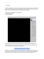
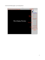
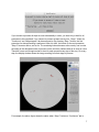
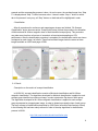
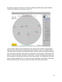
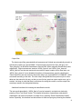
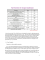
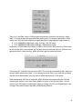
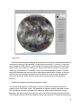
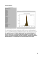
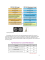
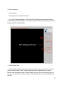
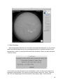
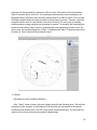
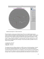
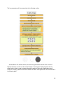
 ASSA GUI User Manual Version 1.12 Last Updated : 2015. 9. 14 1 1. Introduction ASSA is an abbreviation of Automatic Solar Synoptic Analyzer, which is a name of the software system developed by the Korean Space Weather Center of the Radio Research Agency and SELab, Inc in Korea. ASSA consists of the following three categories. 1) sunspot group identification and classification 2) coronal hole detection 3) filament detection For each category, ASSA receives necessary solar raw images and processes them in a designated procedure to yield resultant output files. The whole procedure is performed every hour, and the results are available on following website. http://www.spaceweather.go.kr/models/assa ASSA GUI is a standalone program which enables users to emulate the whole procedures of ASSA in their personal computers. It is developed with IDL and wrapped up as a distributable file package, so that every users can use it even if they don’t have IDL installed on their 2 computer. With this program, users can fully experience the detailed procedures of ASSA. It features algorithms for data receiving, image processing, generating output results, etc.. The current version 1.0 will be continuously updated based on feedbacks from users via this website. 2. Installation ASSA GUI is currently available on Windows and Mac OS X. Users can download the program package on the following link according to each OS. Windows :​
​
http://www.spweather.com/~lee/ASSA/ASSA_WIN32.zip Mac OS X :​
​
http://www.spweather.com/~lee/ASSA/ASSA_MAC64.zip Download the zip file and extract it anywhere you want on your hard drive. Inside the extracted folder, just double click a file named ‘ASSA_MAC64.app’ on Mac OS X or ‘ASSA_WIN32.exe’ on Windows. If you already have IDL 8.x version on your PC, the main GUI will appear. If you don’t have any IDL installed on your PC, ASSA GUI program will be runned under IDL virtual machine environment, thus two splash pop­ups will appear as followings. Just press buttons to continue and the main GUI will appear. If you can see the main GUI which 3 looks like the following figure, you’re ready and set. 4 3. Sunspot Group Detection and Classification 3.1 GUI Interface ­ Description on GUI of sunspot classification In the ‘Sunspot Classification’ tab, you can identify sunspot group and obtain McIntosh and Mt. Wilson magnetic classification results by processing SDO HMI continuum and magnetogram images. The classification algorithms required for this analysis are developed according to the descriptions on sunspot classification presented by SIDC(Solar Influences Data Analysis Center), which is available on the following link. http://sidc.oma.be/educational/classification.php 3.2 Getting Raw Data Date should be specified at the interface for date selection. Year, month, day, hour can be selected for the desired UT date. Any past date may also be selected as far as it can be selected from the pull­down menus. Select the date and time in GUI as the following figure. If you click “Current Date” button, date and time will be automatically set to latest available date and time. Then click “Load Data” button. ASSA program automatically checks the sub­directory called “data” to find out whether the appropriate files already exist. For sunspot classification, ASSA mainly uses SDO HMI solar continuum image(flattened) and magnetogram image named as ● [YYYY][MM][DD]_[hh][mm][ss]_Ic_flat_1k.jpg : continuum image ● [YYYY][MM][DD]_[hh][mm][ss]_M_1k.jpg : magnetogram image Additionally, SRS(Solar Region Summary) data issued daily by NOAA is also required. But in case the SRS data for the selected date is not available yet, the whole process continues without it. If there are no appropriate files in “data” directory, ASSA will show a pop­up window 5 as follows. Then press “OK”, and ASSA will connect to SDO FTP archive and download the files, which are saved in ASSA data diectory(“data”). If you already have such files in your local disk and these files are named appropriately, just copy them to ASSA data directory. It also works. When downloading SDO files is completed, ASSA will show the corresponding continuum and magnetogram images on the main display window as shown in the following figure. You can switch to continuum image or magnetogram image by clicking “Continuum” and “Magnetogram” tabs of Image Tab located at upper­right side of Main Display Window. 3.3 Data Processing ­ Processing continuum and magnetogram images After the appropriate data files are successfully downloaded and displayed, you may choose either to process all steps one by one by pressing each button or to process all steps at once automatically in order, in a pop­up window which looks as follows. Choose an option and press “Continue” button. 6 If you choose to process all steps at once automatically in order, you have only to wait for all processes to be completed. If you choose to process all steps one by one, “Step 1” button for “Continuum” and “Magnetogram” tab becomes active. By pressing “Step 1” button, the first procedure for data processing is performed. After it’s done, the button for the next procedure “Step 2” becomes active, and so on. The remaining buttons become active one by one in order according to the designated order of process, which intuitively indicate what to do next for users. Therefore, users can recognize what is done for each process every step of the way. For every step, the display window shows the image resulting from that stage of process. For example, the above figure shows the status when “Step 6” button on “Continuum” tab is 7 pressed and the corresponding process is done. As can be seen, the resultant image from “Step 6” is displayed and “Step 7” button becomes active. It doesn’t matter “Step 1” button on which tab is first pressed. In any way, all “Step” buttons on both tabs will be highlighted in order. ­ Classification After all procedures for continuum and magnetogram images are finished, “Do Sunspot Classification” button becomes active. Pressing this button invokes the procedure for estimation of McIntosh and Mt. Wilson magnetic class for each identified sunspot group. This procedure may take some time from a few tens of seconds to a few minutes depending on CPU performance. After the classification procedure is completed, the classification results are shown overlapped on each image, as follows. These final resultant images looks the same as those images available on ASSA web page of RRA. 3.4 Result ­ Description on the results of sunspot classification In ASSA GUI, sunspot classification consists of McIntosh classification and Mt. Wilson magnetic classification. The algorithms developed for McIntosh classification is applied to each sunspot group identified on continuum image, in order to determine Zpc class of each group. The algorithms developed for Mt. Wilson magnetic classification is applied to each sunspot group superposed on magnetogram image, in order to determine magnetic class of each group. The basic concept of classifications described by SIDC(Solar Influences Data Analysis Center) in the following link has been mainly referred in order to develop algorithms for classification process in ASSA. http://sidc.oma.be/educational/classification.php 8 The pioneering work of digital implementation of sunspot classification by Colak and Qahwaji (2007) was also referred in developing the classification algorithms for this program. The detailed work flow of both classification process in ASSA is shown in the following figure. As the figure shows, many kinds of quantitative parameters are estimated to be used for class decision. The key parameters will be summarized at the following section. The classification results are overlayed on the final resultant figures. As can be seen in the following figure, the McIntosh class (Zpc) estimated for each sunspot group is written on continuum image with brown colored letters along with the group number. The same kind of information from SRS(Solar Region Summary) issued by NOAA on the same day is also written with green colored letters for comparison. The issue date of SRS used for this figure is written at the bottom with green colored letters. It should be kept in mind that SRS is issued once in a day for 00:30 UT. The date of continuum image used for this analysis is also written at the top with violet colored letters. On the upper left side of the figure, the flare probabilities for C, M, X class are written with black colored letters. On the right bottom side of the figure, the Wolf number is also written with black colored letters. The following formula is used to calculate Wolf number. WN = k(10g+s) s : number of individual sunspots g : number of sunspot groups k : correction factor (assumed to be 1.0) The C, M, X flare probabilities are based on the result of statistical analysis of solar region and 9 flare data for a period of 1996~2011 which was performed by KSWC(Korea Space Weather Center). More details are described in section 3.5. The Mt. Wilson magnetic class estimated for each sunspot group is written on magnetogram image with brown colored letters along with the group number, as seen in the following figure. The same kind of information from SRS(Solar Region Summary) issued by NOAA on the same day is also written with blue colored letters for comparison. The issue date of SRS used for this figure is written at the bottom with green colored letters. The date of magnetogram image used for this analysis is also written at the top with violet colored letters. On the upper left side of the figure, the flare probabilities for C, M, X class are written with black colored letters. On the right bottom side of the figure, the Wolf number is also written with black colored letters. 10 ­ Output files The latest output files generated after all processes are finished are automatically stored in a sub­directory called “gui_figures/ASSA”. Output images are saved as “Spot_Mci.png” and “Spot_Mag.png” for McIntosh classification result and Mt. Wilson magnetic classification result, respectively. Output text data are saved as “ASSA_Spot.txt” and “ASSA_Spot_class.txt”. “ASSA_Spot.txt” has the text resuts such as number of spots, location, area, class letter, etc. “ASSA_Spot_class.txt” more detailed informations of the parameters used for classification. These output files are also stored in directories called “gui_figures/ASSA/YYYY/MM/DD”, which are named according to the date. The other output files generated from previous job for other dates are also stored in this way, so that you can find any previous output results once you’ve worked. Just keep in mind that there’s no buttons for saving the results, as all the output files are always saved in the designated directory. ­ Additional interfaces for browsing the classification results The text results described in “ASSA_Spot.txt” can be browsed in a simple text window by pressing “Show Text Result” button. The detailed information of parameters estimated for classification can also be browsed in a simple GUI by pressing “Show Classification Details” button. Especially, this interface has tab sections for each sunspot group showing the detailed 11 description on how the classification result was derived. Each tab also shows the individual view of the corresponding sunspot group. The following three figures show the examples of these two interfaces for inspecting the classification result more efficienly. ­ Physical parameters As described in the earlier section, there are many parameters derived in the course of classification process in order to make decision in each step. Each parameter has its default value, which is used to produce the public version of figures for classification result which are currently updated at the ASSA website of RRA. These parameters are summarized at the following table. 12 It should be noted that “Show Config” button and its related functionaly for adjusting parameter values are temporarily removed in this version (1.10). This feature will come back with more key parameters available to be adjusted in the upcoming version in near future. It would be helpful to note that such key parameters still can be adjusted by editing the contents of a text file named “config_gui_SC.txt”. But it should be noted that key parameters were determined with our many tests. So please keep in mind that any anomalous results due to changes of such parameters is up to your decision. 3.5 Flare Probability ­ Description on flare probability calculation The C, M, X flare probabilities denoted on the resultant image are based on the result of statistical analysis of solar region and flare data for a period of 1996~2011 which was performed by KSWC(Korea Space Weather Center). For this analysis, past archive of GOES X­ray flare data and McIntosh class data was used to calculate average flare rate for each McIntosh class. This result was then used to determine Poisson flare probabilities for each flare class. The analysis method presented in Bloomfield et al. (2012) was adopted for this work. The entire list of the result is shown in the following figure. 13 On the right bottom section of the resultant figures, flare probabilities for C, M, X class is written with black colored letters. Actually, the probability value for each flare class is a representative value for all sunspot groups on the entire solar disk. This probability for each flare class is calculated according to the following formula. Prob_total = 1 ­ (1­P1)*(1­P2)*(1­P3)*........*(1­Pn) Here n is the number of sunspot groups on the entire solar disk. And each P values are the Poisson probability from the above table. 14 4. Corona Hole Detection 4.1 GUI Interface If you select ‘Coronal Hole Detection’ at Task Tab, GUI for coronal hole detection becomes active, which looks like the following figure. In the ‘Coronal Hole Detection’ tab, you can identify coronal holes by processing SDO AIA 193A and HMI magnetogram images. 4.2 Getting Raw Data Date should be specified at the interface for date selection. Year, month, day, hour can be selected for the desired UT date. Any past date may also be selected as far as it can be selected from the pull­down menus. Select the date and time in GUI as the following figure. If you click “Current Date” button, date and time will be automatically set to latest available date and time. 15 Then click “Load Data” button. ASSA program automatically checks the sub­directory called “data” to find out whether the appropriate files already exist. For sunspot classification, ASSA mainly uses SDO HMI solar continuum image(flattened) and magnetogram image named as ● [YYYY][MM][DD]_[hh][mm][ss]_1024_0193.jpg : AIA 193 image ● [YYYY][MM][DD]_[hh][mm][ss]_HMIB.jpg : magnetogram image Additionally, UCOHO data issued daily by NOAA is also required. But in case the UCOHO data for the selected date is not available yet, the whole process continues without it. If there are no appropriate files in “data” directory, ASSA will show a pop­up window as follows. Then press “OK”, and ASSA will connect to SDO FTP archive and download the files, which are saved in ASSA data diectory(“data”). If you already have such files in your local disk and these files are named appropriately, just copy them to ASSA data directory. It also works. When downloading SDO files is completed, ASSA will show the corresponding AIA 193 and magnetogram images on the main display window as shown in the following figure. You can switch to AIA 193 image or magnetogram image by clicking “AIA 193” and “Magnetogram” tabs of Image Tab located at upper­right side of Main Display Window. 16 4.3 Data Processing After the appropriate data files are successfully downloaded and displayed, you may choose either to process all steps one by one by pressing each button or to process all steps at once automatically in order, in a pop­up window which looks as follows. Choose an option and press “Continue” button. If you choose to process all steps at once automatically in order, you have only to wait for all processes to be completed. If you choose to process all steps one by one, “Step 1” button for “AIA 193” and “Magnetogram” tab becomes active. By pressing “Step 1” button, the first procedure for data processing is performed. After it’s done, the button for the next procedure “Step 2” becomes active, and so on. The remaining buttons become active according to the designated order of process, which intuitively indicate what to do next for users. For every step, the display window shows the image resulting from that stage of process. Therefore, users can recognize what is done for each process every step of the way. For every step, the display window shows the image resulting from that stage of process. For example, the following figure shows the status when “Step 2” button on “AIA 193” tab is pressed and the corresponding process is done. As can be seen, the resultant image from “Step 2” is displayed and “Step 3” button becomes active. It doesn’t matter “Step 1” button on which tab is first pressed. In any 17 way, all “Step” buttons on both tabs will be highlighted in order. 4.4 Result ­ Description on result of corona hole detection After all necessary steps are completed, the final result is displayed by pressing “Show Final Result” button, as seen in the following figure. The polygons with red solid line correspond to the detected coronal holes by ASSA, whereas the polygons with blue solid line correspond to the coronal hole reported by UCOHO data issued for the same day by SWPC. UCOHO results are shown just for comparison. 18 ­ Output files The latest output files generated after all processes are finished are automatically stored in a sub­directory called “gui_figures/ASSA”. Output image is saved as “C_Hole.png”. Output text data is saved as “ASSA_Hole.txt”, which has the text resuts such as number of coronal holes, serial number, area, location of vertices, etc. These output files are also stored in directories called “gui_figures/ASSA/YYYY/MM/DD”, which are named according to the date. The other output files generated from previous job for other date are also stored in this way, so that you can find any previous output results once you’ve worked. Just keep in mind that there’s no buttons for saving the results, as all the output files are always saved in the designated directory. ­ Additional interfaces for browsing the detection results The text results described in “ASSA_Hole.txt” can be browsed in a simple text window by pressing “Show Text Result” button. The distribution of magnetic polarity inside each coronal hole can also be browsed in a simple GUI by pressing “Show Polarity Distribution” button. Especially, this interface has tab sections for each coronal hole showing each distribution plot. The following two figures show the examples of these two interfaces for inspecting the detection 19 result more efficienly. The detailed work flow of coronal hole detection in ASSA is shown in the following figure. It should be noted that the distribution of magnetic polarity inside each candidate area ofcoronal hole is examined. This is based on the final decision method of differentiating coronal holes from filaments, described in Krista and Gallagher (2009). If the skewness of distribution is sufficiently far from zero, the corresponding area can be regarded as a coronal hole. As the work flow in the following figure shows, many kinds of quantitative parameters are estimated to be used for decision. The key parameters will be summarized at the following section. 20 ­ Physical parameters As described in the earlier section, there are many parameters derived in the course of coronal hole detection in order to make crucial decision in some steps. Each parameter has its default value, which is used to produce the public version of figures for classification result which are currently updated at the ASSA website of RRA. These parameters are summarized at the following table. 21 5. Filament Detection 5.1 GUI Interface ­ Description on GUI of filament detection If you select ‘Filament Detection’ at Task Tab, GUI for filament detection becomes active, which looks like the following figure. In the ‘Filament Detection’ tab, you can identify filaments by processing GONG H­alpha images. 5.2 Getting Raw Data Date should be specified at the interface for date selection. Year, month, day, hour can be selected for the desired UT date. Any past date may also be selected as far as it can be selected from the pull­down menus. Select the date and time in GUI as the following figure. If you click “Current Date” button, date and time will be automatically set to latest available date and time. 22 Then click “Load Data” button. ASSA program automatically checks the sub­directory called “data” to find out whether the appropriate files already exist. For sunspot classification, ASSA mainly uses H­alpha image from Big Bear or Learmonth or El Teide named as ● [YYYY][MM][DD][hh][mm][ss]Bh.jpg : H­alpha image from Big Bear ● [YYYY][MM][DD][hh][mm][ss]Lh.jpg : H­alpha image from Learmonth ● [YYYY][MM][DD][hh][mm][ss]Th.jpg : H­alpha image from El Teide The choice of image file to be downloaded depends upon the operation hour of each observatory. The coverage hour for Big Bear data is 16~23 UT, 00~07 UT for Learmonth, and 08~15 UT for El Teide. It should be noted that only those image files for available hours can be downloaded. If there are no appropriate data files in “data” directory, ASSA will show a pop­up window as follows. Then press “OK”, and ASSA will connect to GONG H­alpha FTP archive and download the files, which are saved in ASSA data diectory(“data”). If you already have such files in your local disk and these files are named appropriately, just copy them to ASSA data directory. It also works. When downloading H­alpha files is completed, ASSA will show the corresponding H­alpha raw image on the main display window as shown in the following figure. 23 5.3 Data Processing After the appropriate data files are successfully downloaded and displayed, you may choose either to process all steps one by one by pressing each button or to process all steps at once automatically in order, in a pop­up window which looks as follows. Choose an option and press “Continue” button. If you choose to process all steps at once automatically in order, you have only to wait for all processes to be completed. If you choose to process all steps one by one, “Step 1” button for “AIA 193” and “Magnetogram” tab becomes active. By pressing “Step 1” button, the first 24 procedure for data processing is performed. After it’s done, the button for the next procedure “Step 2” becomes active, and so on. The remaining buttons become active according to the designated order of process, which intuitively indicate what to do next for users. For every step, the display window shows the image resulting from that stage of process. Therefore, users can recognize what is done for each process every step of the way. For every step, the display window shows the image resulting from that stage of process. For example, the following figure shows the status when “Step 2” button is pressed and the corresponding process is done. As can be seen, the resultant image from “Step 2” is displayed and “Step 3” button becomes active. Likewise, all “Step” buttons will be activated in order. 5.4 Result ­ Description on result of filament detection After “Step 5” button is press, the result typically looks like the following figure. The red lines correpsond to the “skeleton” of each filament, with the black dots correspond to the vertices connecting such skeleton lines. This is the main result of filament detection. The next and final result is just a mixture of this and the masked H­alpha image. 25 The final result of filament detection is displayed by pressing “Show Final Figure” button, as seen in the following figure. ­ Output files The latest output files generated after all processes are finished are automatically stored in a sub­directory called “gui_figures/ASSA”. Output image is saved as “Filaments.png”. Output text data is saved as “ASSA_Filaments.txt”, which has the text resuts such as number of filaments, serial number, length, location of vertices, etc. These output files are also stored in directories called “gui_figures/ASSA/YYYY/MM/DD”, which are named according to the date. The other output files generated from previous job for other dates are also stored in this way, so that you can find any previous output results once you’ve worked. Just keep in mind that there’s no buttons for saving the results, as all the output files are always automatically saved in the designated directory. 26 ­ Additional descriptions on filament detection Filament detection requires ground H­alpha image. There’s no H­alpha images not only routinely observed by satellite but also being provided to the public in realtime. GONG H­alpha archive provides near realtime H­alpha data observed at some representative ground solar observatories. The available observing hour differs from observatory to observatory. In ASSA system, H­alpha images from Big Bear, Learmonth and El Teide Solar Observatory are used, because their entirely different time coverage in UT(as follows) makes it possible to cover as many hours as possible. (1) Learmonth : 00~07 UT (2) El Teide : 08~15 UT (3) Big Bear : 16~23 UT The detailed work flow of filament detection in ASSA is shown in the following figure. It should be noted that morphology opening plays a very important role in discriminating features of elongated shape typical of filaments. For this purpose, structuring elements of elongated shape with various direction angles are used for morphological opening (Shih and Kowalsky 2003). As the figure shows, many kinds of quantitative parameters are estimated to be used for decision. 27 The key parameters will be summarized at the following section. As described in the earlier section, there are many parameters derived in the course of filament detection in order to make crucial decision in some steps. Each parameter has its default value, which is used to produce the public version of figures for classification result which are currently updated at the ASSA website of RRA. These parameters are summarized at the following table. 28 ● References 1. Bloomfield, D. S., Higgins, P. A., McAteer, R. T. J., Gallagher, P. T., ApJL, 747, L41, 2012 2. Colak, T., and Qahwaji, R., Solar Physics, 248, 277, 2007 3. Krista, L. D. and Gallagher, P. T., Solar Physics, 256, 87, 2009 4. Shih, F. Y. and Kowalsky, A. J., Solar Physics, 218, 99, 2003 ● Acknowledgement License This software was developed at the Korean Space Weather Center of the Radio Research Agency by SELab, Inc. This software is a freeware. It is an experimental system and RRA assumes no responsibility whatsover for its use by other parties, and make no guarantees. Contact : Address: 198­6, Gwideok­ro, Hallim­eup, Jeju­si, Jeju­do 695­922 Korea Phone: +82­64­797­7031 Email: [email protected] feedback site : http://www.spaceweather.go.kr/assa 29 <Update note on version 1.12> 1. For filament detection, the list of H­alpha observation sites was changed (Big Bear, Udaipur ==>> Big Bear, Learmonth, El Teide) 2. Algorithms for filament detection was slightly modified to be compatible with the new data list 3. Some minor bug issues are fixed <Update note on version 1.10> 1. FL processing for filament detection is now fully supported 2. Download link for AIA 193 images for CH detection has been changed 3. Problem of Alpha­Delta has been fixed 4. SC output files are now produced even when there’s no sunspot at all 5. Flare probabilities shown on SC output files are now estimated based on the statistical analysis of the dependence of flaring probability on Zpc class obtained by applying ASSA algorithm to past archive of SOHO data archive (1996~2011) 6. N­S separation between sunspots are also considered in sunspot grouping 7. Problem of too many ‘C’ of Z class value has been fixed 8. Problem of multiple ROIs in disk masking has been fixed 9. Problem of showing wrong rectangular sector in ‘Show Classification Details’ interface has been fixed 10. Hole­shaped ROIs with minus area are now can be excluded 12. Many changes of internal algorithms as of September 2014 were fully applied 13. Screen size of main GUI is automatically adjusted by adopting scroll bars 14. Other minor problems are has been fixed <Update note on version 1.07> 1. Pressing 'Load Data' button launches a pop­up window for choice between two options of processing ("Step By Step" or "All Steps At Once"). It should be noted that "All Steps At Once" processes all steps at once without pressing each step button, but each step button doesn't become active after finish. 2. Two kinds of area are measured for each sunspot group. One is a sum of areas of all sunspots, the other is a sum of areas of only the sunspots with penumbra. These two kinds of areas are recorded in the resultant text file (ASSA_spot.txt). 3. Longitudinal extent of each sunspot group is added to the contents of the resultant text file (ASSA_spot.txt). 4. Magnetogram image of each sunspot group can also be shown on 'Show Classification Details' interface, in addition to continuum image. 5. Numbering order of sunspot groups is reversed (W­>E) 6. Some minor bug issues are fixed. <Update note on version 1.03> 1. Method of calculating flare probabilities for entire solar disk has been changed. 2. Problem of estimating sunspot group area based on morphology close method has been fixed. 30 3. Problem of image view of sunspot group located near disk limb on 'Show Classification Details' interface has been fixed. 4. Problem of adjusting 'maximum separation between two spots' on 'Show Config' interface has been fixed. 5. Background color of task title string on Windows GUI is now the same as GUI background color. 6. Detected sunspot groups are now numbered according to its heliographic longitude. 7. Some minor issues are fixed. 31