1
New Directions for Surface Water ModelingCProceedings of the Baltimore Symposium, May 19891
IAHSPubl.no. 181,1989.
A modular model for simulating continuous or event runoff
D. Stephenson
Water Systems Research Group,
Johannesburg, South Africa
University
of
the
Witwatersrand,
ABSTRACT
A review of stormwater model arrangements is made.
Computer programs able to assemble loosely-connected elements are
simplest to use and understand. Arrangement of elements and assembly
in parallel or series enables all possible types
of models to be
accommodated. Hydraulic elements are used
for surface runoff
visualization and groundwater aquifers are simulated in parallel for
continuous or long term simulations.
INTRODUCTION
The accuracy of runoff models can be improved at the expense of more
and more data. There are many models available with differing levels
of sophistication for such studies. The author contends however the
biggest cost of modelling is often in learning the ins and outs of a
model, and its principles and limitations. On the lower levels of the
learning curve many users may wish to dabble with a model, and at the
upper end there are many technical aspects to remember. Time away
from the model causes users to forget aspects, and it is the ease of
initial or re-access which can inspire confidence in the user and
enable the model to be used to its fullest. Various types of models
are discussed bearing these points in mind.
Sub catchment arrangement
The interconnection of one sub-catchment or element with another can
be done in various ways (Fig. 1 ) :
i)
ii)
iii)
Finite difference grids In the case of a homogeneous type
catchment a rectangular grid can be superimposed. Thus flows
and water depths are computed at grid point. Either one or two
directional flow can be assumed. In general two flow vectors
must be assumed. An exception occurs if the flow is in one
direction parallel to one of the axes. For most undular
topography two-dimensional analysis is necessary.
Finite element The computations can be reduced and size and
shape of element varied to suite the topography if a finite
element approach is used. In general a two-direction flow
pattern must be assumed although if the boundaries of elements
are perpendicular to flow, one-directional flow can be assumed.
Modular The simplest and most versatile model is one made up of
modules which can be linked up at the ends. Generally the flow
is one directional along the axis but two dimensional
catchments can be made up of modules in parallel and series,
i.e. the orientation of the module is ignored because the
directional momentum of the water is not considered. It is the
latter configuration en which the model describes here is
based.
83
D. Stephenson
84
LONG
FLOW
DIRECTION
f
ALTERNATIVE , 2 - d FLOW
NEW SPACE GRID POSITON
6-
BACK BOUNDARY
LATERAL DISTANCE x
(a)
Finite difference grid
ALTERNATIVE, 2 - d
(b)
OUT-FLOW
Finite eiements
3
2
1
Cc)
Modules
Fig. 1 Alternative grids.
THEORETICAL BASIS
Hydrologioal models range from statistical to conceptual, embracing
probabilistic, curve fitting, black boxes, analogous e.g. cell type
(Diskin et al 1984), through to the more hydrodynamically correct.
Even the latter range from simplistic e.g. time area (Watson, 1981)
though first approximation kinematic type, diffusion equations and
hydrodynamic equations (SWMM, Huber et al, 1982). The latter are only
necessary for surface runoff simulation and even then are not always
warranted. For runoff determination accelerations and backwater
effects are not significant. On the other hand the time-area approach
which derived from the rational method, does not accommodate the
effect of water depth on concentration time. Mono time axes and
linear rainfall-runoff relationships have been taken to their extreme
in unit hydrograph theory, and as a result the hydraulic basis is
often overlooked in sophisticated models e.g. OTTHYMO (Wisner, 1980).
85
A modular model for simulating continuous or event runoff
It is into the more hydraulically based models that the majority
of research is now directed. By suitable selection of module
arrangement, one-dimensional flow can be assumed, i.e. the module
axis is taken in the general flow direction. Lateral flow time is
neglected, (which could introduce error in flood plane type modules).
Transverse i.e. lateral and vertical (for horizontal flow direction)
accelerations are also neglected but this is quite satisfactory for
all runoff modelling (see Fig. 2 ) .
Thus the hydrodynamic equations are narrowed down to the St.
Venant equations and their derivatives. Accelerations are not of
importance in overland or long river studies so these terms are
omitted, and backwater effects are only of importance in some channel
situations, so most modules are limited to kinematic type equations.
Flow is assumed uniform down the reach. That is, the water depth
is constant down the reach. There may be local backup which does
affect system storage however. Since inflow is thus spread over the
full length of a reach each time step, the routing effect can be
unrealistic unless the time step is sufficiently large. Methods of
minimizing numerical routing (or using it to approximate time
routing) have been investigated (Holden and Stephenson, Ï988).
LATERAL FLOW
MAIN
CHANNEL
ANOMALY
1
WITH
KINEMATIC
FLOW
ANOMALY
2
KITH
KINEMATIC
FLOW
Fig. 2 Problems with specific numerical methods.
D. Stephenson
86
It should be noted the kinematic assumption of energy gradient
parallel to conduit bed can cause complications at changes in slope.
Depressions do not correctly store inflow, and separate storage
modules are necessary.
CONTINUOUS SIMULATION
Groundwater flow capability with aquifer modules makes possible long
term simulation of catchment yield. Groundwater contributions lag
surface runoff by hours or even months. Recession limbs of stormwater
hydrographs can be due to contributions from perched water tables or
interflow. Longer term yields are from deeper aquifers.
Recharge of surface layers is however important from the point of
view of antecedent moisture and permeability for forthcoming storms.
The continuous simulation capability therefore improves estimation of
surface storm runoff. Surface layer moisture is also important for
estimating evaporation and losses.
The time scale of flow from deeper aquifers may be much longer
than from the higher water tables, and a greater time step could be
used once surface runoff is reduced.
The problem then arises as to future storm problems and their
infiltration. However from the total yield point of view it is not
critical if storm patterns are assumed.
ROUTING PROCESS
Kinematic waves are theoretically not subject to diffusion i.e.
spreading and attenuation, as no dynamic effects are included in the
equation. There may be changes in wave shape since dx/dt is a
function of depth, but there can be no change in peak flow unless
there is an inflow. The advantage of taking large distance increases
with the kinematic method therefore results in a sacrifice in
accuracy. Holden and Stephenson
(1988) proposed a method for
minimizing the numerical error and getting the best approximation to
hydrodynamic diffusion.
The wave diffusion can be accounted for using the slightly more
accurate equations, namely the diffusion equations, or the full
dynamic equations. However in some cases wave diffusion can be
reproduced numerically. From the mathematical point of view,
numerical diffusion can be controlled or minimised. Explicit solution
of the kinematic equations is often employed in preference to
implicit solution as the friction equation is non-linear, and
explicit schemes such as the backward centred, or semi explicit such
as the 4-point scheme of Brakensiek (1967) are reasonably accurate
and fast. Explicit schemes can be subject to numerical instability
unless the time increment is small enough, i.e. A t < Ax/(dx/dt), (the
Courant criterion) where dx/dt =
a my
. O n the other hand the
smaller At the greater the numerical diffusion as the numerical
effect travels at.a speed Ax/At. The optimum compromise is for Ax/At
= dx/dt. This is not always possible in an equispaced grid as dx/dt
varies. Ponce (1986) attempted to reproduce actual diffusion in
kinematic equations by writing the finite difference equations for
flow in a way similar to the Muskingum-Cunge routing equation.
Adopting a more practical approach the kinematic diffusion
process can be explained as follows. The routing process which occurs
with kinematic modelling is similar to reservoir routing where
discharge depends only on the stage at the outlet. A unique stage
87
A modular model for simulating continuous or event runoff
discharge relation is assumed i.e. no allowance is made for
accelerations or water surface gradient. A compromise could be made
by setting discharge a function oi stage at more than one point e.g.
average of upstream and downstream stages.
The resulting effect is similar to that employed in the Muskingum
method
and
in
addition
allows
for
non-linearity
in
the
stage-discharge relationship. It also has the advantage that the
parameters in the equations are physically measurable and not
empirical. To overcome the non-linear relationships the kinematic
equations can be solved in two steps, namely the continuity equation
to determine change in water depth, and discharge is obtained from
stage using the selected discharge equation.
The discharge equation is not limited to a channel type equation
such as that of Manning. Thus using a general discharge equation of
the form
Q = Kh m
if h is stage at discharge point and m = 5/3, one has the Manning
equation, if m = 5/2 one has a triangular weir, m = 3/2 is a
rectangular weir, m = 1/2
is an orifice and m = 1 is a deep
rectangular channel. If h is the difference between upstream and
downstream stages, then if m = 1/2 one has turbulent pipe flow, and
if m = 1 one has laminar flow in a closed conduit or contained
aquifer.
MANAGEMENT CAPABILITY
A drawcard of a model prepared on the above lines WITSKM (WITS STORM
KINEMATIC MODULAR MANAGEMENT MODEL) is its versatility when it comes
to redirecting flows and attenuating hydrographs. The facility of
readily being able to redirect flows along different routes means
channel storage or open versus closed conduit conveyance can be
explored. The re-routing of flows along circuitous routes may
increase channel storage. This in turn increases concentration time
and could reduce design peak flows. New townships layouts could be
varied until a suitable stormwater drainage pattern emerged.
The overflow facility also enables dual drainage to be used to
maximum advantage. Excess flow could be led to shallow channels (or
roadways) which will provide retardation or lead to channels which
are only used in emergencies, the overflow level can readily be
varied to permit difference risk storms to be accommodated in the
minor (underground conduit) system.
The aquifer option is also of use in urban catchment management
studies. Aquifers can be recharged by direct infiltration or with
water led to them from less pervious areas. In either case the
absorption of the aquifer is only limited by the depth-discharge
characteristics and initial moisture conditions.
A useful module for hydrograph attenuation is the storage module.
Reservoir surface area, dead storage and overspill crest level can be
varied to achieve an optimum balance between maximum water depth and
dam cost. The ability to vary the outlet discharge characteristic is
however the most versatile facility of the storage module. By means
of a general discharge equation of the form
Q = (WA)ym
any form of outlet control can be • used. For example an orifice is
represented if m = 1/2 and WA = Ca \/(2g),
where C is a discharge
coefficient, a is the orifice cross-sectional area and g is gravity.
For detention attenuation which has a decreasing effect with
D. Stephenson
88
inflow, m should be high and for high detention at all depths m
should be small. Again by trial, an optimum compromise between dam
cost and cost of conveying away the discharge can be achieved.
MODULES
The versatility of the computer programme is enhanced by the
possibility of fitting in various types of hydrological units or
modules into a system. Catchments, aquifers, conduits and storage
basins can be linked in any order. The various modules which can be
built-in are as follows (Fig. 3 ) .
I I I II I
I I I I I I
M ! I I 1
5
JlSiIIiii! w
E
2
Fig. 3 Graphs output for connectivity check.
Catchments
A basic catchment is a rectangular shape sloping in one direction.
The module reference number, its downstream module, initial water
depth, length, width and discharge coefficient (ratio of discharge to
depth to the power of 5/3) e.g. \/(S/n) where S is gradient and n is
Manning roughness, are required as input data. In addition the
surface permeability, suction at the ground wetting front, initial
moisture content and aquifer module number are required. An
infiltration process based on the soil physics model of Green and
Ampt (1911) is assumed.
Catchments can be linked in cascades (in series) for example
changing slopes or disconnected impervious surface, or in parallel,
for instance if portion has directly connected impermeable cover.
Circular conduits (pipes)
Urbanized catchments are normally sewered with underground pipes,
which run part full for most of the time. When they surcharge, the
89
A modular model for simulating continuous or event runoff
excess flow continues down roads and may be directed to channels.
Such a system ("major/minor" system) is common at high flows whether
intentional or not and provides roads free of ponding for all but
exceptional storms. The capability of modelling such systems is
therefore important.
Data required for this type of module are module reference
number,
downstream
module,
initial
depth,
length,
diameter,
conveyance (\/(S/n)), and overflow module number.
Trapezoidal channels
Open channels are the most common conduits, be they roadways,
gutters, ditches or canals. Where the channel is a simple trapezoid,
the data requirements are limited to module reference number,
downstream
module,
initial
flow
depth,
length, base
width,
conveyance, size slopes, maximum depth and overflow module.
Compound channels
Natural channels may be defined using an arbitrary number of
co-ordinates
across a section. The
stream
between
any
two
neighbouring points is treated as an independent section so that
velocity varies depending on flow depth and roughness. Flood planes
are thus accommodated with slow moving storage on the banks and a
more rapid stream between banks.
Data are module reference number, downstream module, initial
depth, length, slope, points, co-ordinates and roughness of each
section.
This facility can be used to calculate normal depth in compound
channels. An impermeable catchment upstream with an area of 3600m x
100m is fed with Rmm of catchment rain (where R is normal flow in
m 3 /s) and after a period of time the depth in the downstream channel
stabilizes at normal depth.
Storage basins
Where detention of retention is required, on- or off- channel storage
may be of use.
Data required are module reference number, downstream module,
initial water depth, length, width, conveyance a, discharge depth
coefficient m(Q = Way ), side slope of basin, dead storage before
discharge, and crest level of dam wall. By experimenting with the
outlet e.g. crest or orifice spillway, a best design may be achieved.
Aquifers
Water may infiltrate to aquifers from catchments or be discharged
directly into them from .any conduit or overflow. The aquifer acts as
a conduit albeit with a much slower flow rate. The aquifer will also
have a maximum depth and may leak to a lower aquifer. Stacking or
cascading of aquifers is possible. The kinematic equations are
entirely adequate for this type of flow as dynamic effects are
absent.
Data include aquifer reference number, downstream module number,
initial flow depth, length, width, conveyance defined as kS where k
is permeability and S is gradient, porosity, aquifer depth and
underneath aquifer number.
D. Stephenson
90
OTHER FACILITIES
A frequent source of error in stormwater programs arise when
downstream catchment number is changed or forgotten. A facility
exists for displaying graphically on a PC colour screen the entire
network once it is entered on the computer. Each module is drawn
according to the type e.g. pipe, catchment, channel, and is connected
upstream and downstream as indicated in the data. Overflow routes are
also indicated. In general
the model is designed
for easy
understanding and input and cross checking. It is especially useful
for stormwater management studies. The groundwater modules enable
continuous simulation to be performed, which
is useful
for
establishing antecedant moisture conditions for storms, and dry
weather flows (Fig. 4 ) .
GOOD PRACTICE
BAD PRACTICE
DISCONNECTED IMPERVIOUS AREA
DETENTION STORAGE
DUAL
DRAINAGE
Fig. 4 Management methods investigated with model.
91
A modular model for simulating continuous or event runoff
REFERENCES
Brakensiek, D.L. (1967)
Kinematic flood routing. Trans. Am. Soc. Agr. Engrs. 10(3), pp
340-343.
Diskin, M.H., Wyeseure, G. and Fayen, J. (1984)
Application of a cell model to the Bellebeek watershed. Nordic
Hydro]., 15.
Green, W.H. and Ampt, G.A. (1911)
Studies of soil physics, 1, the flow of air and water through
soils. J. Agric. Science, 4(1), p 1-24.
Holden, A.P. and Stephenson, D. (1988)
Improved 4-point solution of the kinematic equations. J. IAHR,
26(4), 1-11.
Huber, W.C. Heaney, J.P., Nix, S.J., Dickenson, P.E. and Pilman, D.J.
(1982)
Stormwater Management Models, User Manual, Dept. Environ. Eng.
Sciences, Univ. of Florida.
Ponce, V.M. (1986)
Diffusion wave modelling of catchment
dynamics. Journal
of
Hydraulic Engineering. ASCE, 112(8), pp 716-727.
Watson, M.D. (1981)
Application of Illudas to stormwater drainage design in S.A..
Hydrol. Res. Unit. University of the Witwatersrand.
Wisner, P.E. (1980)
0TTHYM0, A planning model for master drainage plans in urban areas.
Toronto.