Download Installation Manual and User Guide

MAGNEFORCE SOFTWARE SYSTEMS, INC.
BLDC
Installation Manual
and User Guide
BLDC Installation Manual & User
Guide
© MagneForce Software Systems, Inc.
P.O. Box 4652
Timonium, MD 21094
Phone 716.646.8577 • Fax 716.646.1973
Copyright
Copyright 2001
MagneForce Software Systems, Inc.
All rights reserved
First printing, November 2001
MagneForce Software Systems, Inc.
P.O. Box 4652
Timonium, MD 21094
(716) 646-8577
STATEMENTS IN THIS DOCUMENT REGARDING THIRD PARTY
STANDARDS OR SOFTWARE ARE BASED UPON INFORMATION MADE
AVAILABLE BY THIRD PARTIES. MAGNEFORCE AND ITS AFFILIATES ARE
NOT THE SOURCE OF SUCH INFORMATION AND HAVE NOT
INDEPENDENTLY VERIFIED SUCH INFORMATION. THIS DOCUMENT IS
SUBJECT TO CHANGE WITHOUT NOTICE.
Trademarks
MagneForce, its logo and BLDC are registered trademarks and/or registered service
marks of MagneForce Software Systems, Inc.
Other parties’ trademarks or service marks are the property of their respective owners
and should be treated as such.
License
This Manual and the software described within is furnished under license and may only
be used or copied in accordance with the terms of such license. The information in this
manual is furnished for informational use only, is subject to change without notice, and
should not be construed as a commitment by MagneForce Software Systems, Inc.
MagneForce assumes no responsibility or liability for any errors or inaccuracies that may
appear in this book.
Limit of Liability/Disclaimer of Warranty
MagneForce has used its best efforts in preparing this software and manual. MagneForce
makes no representations or warranties with respect to accuracy or completeness.
MagneForce Software Systems, Inc. 2002 Software License Agreement
Software is defined as the MagneForce Software Systems, Inc.
(MagneForce) computer program with which this Software License
Agreement is included and any updates or maintenance releases thereto.
The use by You of any services or content accessible through the
Software may be subject to your acceptance of separate agreements with
MagneForce or third parties. This Agreement applies to all standard
versions of the Software and other branded or customized versions
unless otherwise agreed. Do not use the Software until you have
carefully read the following Agreement. This Agreement sets forth the
terms and conditions for licensing of the Software from MagneForce to
you, and installing and using the Software indicates that you have read
and understand this Agreement and accept its terms and conditions. If
you do not agree with this Agreement, promptly return the Software and
accompanying items to the place of purchase, or as provided below,
within sixty (60) days of purchase for a full refund.
License and Certain Restrictions
Trial Versions
If this Agreement is included with the trial versions of the Software, you
are granted a limited non-exclusive license to use a copy of the enclosed
Software for the specified number of uses or until the trial expiration
date has been reached, in the materials accompanying the trial versions
of the Software: (i) if using the single-user trial version, on a computer
used by a single individual. Thereafter, you may purchase the right to use
the appropriate full version of either the single-user or multi-user
versions of the Software which license terms are specified below, by
contacting MagneForce or your retailer. You may not copy the printed
materials accompanying the Software if any, or print multiple copies of
any user documentation. BY YOUR USE OF THE TRIAL VERSION
OF THE SOFTWARE YOU UNDERSTAND AND AGREE THAT
AFTER A CERTAIN DATE, YOU MAY NOT BE ABLE TO
CONTINUE TO ACCESS AND/OR USE THE SOFTWARE OR
ANY DATA YOU HAVE ENTERED INTO SUCH SOFTWARE
UNLESS YOU PURCHASE THE APPROPRIATE FULL VERSION
OF THE SOFTWARE.
Single-User Version
If you purchased a full, single-user version of the Software, you are
granted a limited non-exclusive license to use a copy of the enclosed
Software on the computer(s) used by a single individual. You may make
one (1) backup copy of the Software for your own use. You may not
copy the printed materials accompanying the Software if any, or print
multiple copies of any user documentation.
General
Making additional copies of the Software, or enabling others to use your
registration code(s), license file(s), security key(s) or serial number(s), if
any, is strictly prohibited. It is also prohibited to give copies to a person
who has not purchased the appropriate license for the Software from
MagneForce; to install the Software on computers used by individuals
who have not purchased the appropriate licenses for the Software from
MagneForce; or to duplicate the Software by any other means including
electronic transmission. The Software in its entirety is protected by the
copyright laws. The Software also contains MagneForce trade secrets,
and you may not decompile, reverse engineer, disassemble, or otherwise
reduce the Software to human-perceivable form or disable any
functionality which limits the use of the Software. You may not modify,
adapt, translate, rent or sublicense (including offering the Software to
third parties on an applications service provider or time-sharing basis),
assign, loan, resell for profit, or distribute the Software, disk(s), or related
materials or create derivative works based upon the Software or any part
thereof. You may not network the Software.
Termination
This Agreement may be terminated by MagneForce immediately and
without notice if you fail to comply with any term or condition of this
Agreement. Upon such termination, you must immediately destroy all
complete and partial copies of the Software, including all backup copies.
From time to time, MagneForce may change the terms and conditions of
this Agreement. MagneForce will notify you of any such change. For
the latest version of this Agreement, go to www.magneforcess.com, or
such other site designated by MagneForce. Your continued use of this
Software will indicate your agreement to the change.
Satisfaction Guaranteed
If you are not 100% satisfied with this Software, MagneForce's entire
liability and your exclusive remedy shall be return of the Software within
sixty (60) days of purchase to MagneForce Returns, P.O. Box 4652
Timonium, MD 21094 for such refund; or (2) return the Software within
sixty (60) days of purchase, to MagneForce Returns at the above address
for replacement of defective disks. If the disks are defective and you
would like replacement disks while this version is still commercially
available after sixty (60) days from date of purchase, you may obtain a
replacement by sending your defective disks and a check for thirty-five
dollars ($35.00), plus applicable tax, to MagneForce.
DISCLAIMER OF WARRANTIES
EXCEPT AS PROVIDED ABOVE, THIS SOFTWARE AND ANY
RELATED SERVICES OR CONTENT ACCESSIBLE THROUGH
THE SOFTWARE ARE PROVIDED "AS-IS," AND TO THE
MAXIMUM EXTENT PERMITTED BY APPLICABLE LAW,
MAGNEFORCE DISCLAIMS ALL OTHER REPRESENTATIONS
AND WARRANTIES, EXPRESS OR IMPLIED, REGARDING
THIS SOFTWARE, DISKS, RELATED MATERIALS AND ANY
SUCH SERVICES OR CONTENT, INCLUDING THEIR FITNESS
FOR A PARTICULAR PURPOSE, THEIR QUALITY, THEIR
SECURITY,
THEIR
MERCHANTABILITY,
OR
THEIR
NONINFRINGEMENT. MAGNEFORCE DOES NOT WARRANT
THAT THE SOFTWARE OR ANY RELATED SERVICES OR
CONTENT IS FREE FROM BUGS, VIRUSES, ERRORS, OR
OTHER PROGRAM LIMITATIONS NOR DOES MAGNEFORCE
WARRANT ACCESS TO THE INTERNET OR TO ANY OTHER
SERVICE OR CONTENT THROUGH THE SOFTWARE. SOME
STATES DO NOT ALLOW THE EXCLUSION OF IMPLIED
WARRANTIES, SO THE ABOVE EXCLUSIONS MAY NOT
APPLY TO YOU. IN THAT EVENT, ANY IMPLIED
WARRANTIES ARE LIMITED IN DURATION TO SIXTY (60)
DAYS FROM THE DATE OF PURCHASE OF THE SOFTWARE.
HOWEVER, SOME STATES DO NOT ALLOW LIMITATIONS
ON HOW LONG AN IMPLIED WARRANTY LASTS, SO THE
ABOVE LIMITATION MAY NOT APPLY TO YOU. THIS
WARRANTY GIVES YOU SPECIFIC LEGAL RIGHTS, AND YOU
MAY HAVE OTHER RIGHTS AS WELL, WHICH VARY FROM
STATE TO STATE.
LIMITATION OF LIABILITY AND DAMAGES
THE ENTIRE LIABILITY OF MAGNEFORCE AND ITS
REPRESENTATIVES (AS DEFINED BELOW) FOR ANY
REASON SHALL BE LIMITED TO THE AMOUNT PAID BY THE
CUSTOMER FOR THE SOFTWARE UNLESS OTHERWISE
SEPARATELY AGREED. TO THE MAXIMUM EXTENT
PERMITTED BY APPLICABLE LAW, MAGNEFORCE AND ITS
SUBSIDIARIES, AFFILIATES, LICENSORS, PARTICIPATING
FINANCIAL INSTITUTIONS, THIRD-PARTY CONTENT OR
SERVICE PROVIDERS, DISTRIBUTORS, DEALERS OR
SUPPLIERS ("REPRESENTATIVES") ARE NOT LIABLE FOR
ANY
INDIRECT,
SPECIAL,
INCIDENTAL,
OR
CONSEQUENTIAL DAMAGES (INCLUDING, BUT NOT
LIMITED TO: DAMAGES FOR LOSS OF BUSINESS, LOSS OF
PROFITS OR INVESTMENT, OR THE LIKE), WHETHER BASED
ON BREACH OF CONTRACT, BREACH OF WARRANTY, TORT
(INCLUDING NEGLIGENCE), PRODUCT LIABILITY OR
OTHERWISE,
EVEN
IF
MAGNEFORCE
OR
ITS
REPRESENTATIVES HAVE BEEN ADVISED OF THE
POSSIBILITY OF SUCH DAMAGES, AND EVEN IF A REMEDY
SET FORTH HEREIN IS FOUND TO HAVE FAILED OF ITS
ESSENTIAL PURPOSE. SOME STATES DO NOT ALLOW THE
LIMITATION AND/OR EXCLUSION OF LIABILITY FOR
INCIDENTAL OR CONSEQUENTIAL DAMAGES, SO THE
ABOVE LIMITATION OR EXCLUSION MAY NOT APPLY TO
YOU. THE LIMITATIONS OF DAMAGES SET FORTH ABOVE
ARE FUNDAMENTAL ELEMENTS OF THE BASIS OF THE
BARGAIN
BETWEEN
MAGNEFORCE
AND
YOU.
MAGNEFORCE WOULD NOT BE ABLE TO HAVE PROVIDED
THIS
SOFTWARE
OR
SERVICES
WITHOUT
SUCH
LIMITATIONS.
U.S. Government
The Software is a "commercial item," as that term is defined at 48 C.F.R.
2.101 (OCT 1995), consisting of "commercial computer software" and
"commercial computer software documentation," as such terms are used
in 48 C.F.R. 12.212 (SEPT 1995) and the Department of Defense
Federal Acquisition Regulations Sections 252.227-7014 (a) (1), (5).
Consistent with 48 C.F.R. 12.212 and 48 C.F.R. 227-7202-1 through
227-7202-4 (JUNE 1995), all U.S. Government End Users acquire the
MagneForce software (or Licensed Product) with only those rights set
forth herein. MagneForce Software Systems, Inc., P.O. Box 4652,
Timonium, MD 21094.
Export Restrictions
You acknowledge and agree that the MagneForce Software is subject to
restrictions and controls imposed by the Export Administration Act and
the Export Administration Regulations ("the Acts"). You agree and
certify that neither the MagneForce Software nor any direct product
thereof is being or will be used for any purpose prohibited by the Acts.
You agree and certify that you are not a citizen or permanent resident of
the following countries: Cuba, Iran, Iraq, North Korea, Libya, Sudan or
Syria.
General Provisions
This Agreement sets forth MagneForce's and its Representatives' entire
liability and your exclusive remedy with respect to the Software. You
acknowledge that this Agreement is a complete statement of the
agreement between you and MagneForce with respect to the Software,
and that there are no other prior or contemporaneous understandings,
promises, representations, or descriptions with respect to the Software.
This Agreement shall govern any services or content related to the
Software, unless such services or content are subject to a separate written
agreement between you and MagneForce or its Representatives.
However, the limitations of liability and disclaimer of warranties in this
Agreement shall apply to MagneForce and its Representatives with
respect to such content or services except to the extent provided
otherwise in a separate written agreement approved by MagneForce
between you and MagneForce or the applicable Representative(s).
This Agreement does not limit any rights that MagneForce may have
under trade secret, copyright, patent, or other laws. The Representatives
of MagneForce are not authorized to make modifications to this
Agreement, or to make any additional representations, commitments, or
warranties binding on MagneForce, other than in writing signed by an
officer of MagneForce. Accordingly, such additional statements are not
binding on MagneForce and you should not rely upon such statements.
If any provision of this Agreement is invalid or unenforceable under
applicable law, then it is, to that extent, deemed omitted and the
remaining provisions will continue in full force and effect. The validity
and performance of this Agreement shall be governed by Maryland law
(without reference to choice of law principles), except as to copyright
and trademark matters, which are covered by federal laws. This
Agreement is deemed entered into at Timonium, Maryland, and shall be
construed as to its fair meaning and not strictly for or against either
party.
Consumer Information and Privacy
For details about MagneForce's privacy policies, please refer to the
MagneForce Privacy Statement contained either in the Software or on a
website designated by MagneForce.
MagneForce, the MagneForce logo, BLDC, and BLDC, among others,
are registered trademarks and/or registered service marks of
MagneForce Inc. in the United States and other countries.
MagneForcess.com, among others, is a trademark and/or service mark
of MagneForce Software Systems, Inc. in the United States and other
countries. Other parties' trademarks or service marks are the property of
their respective owners and should be treated as such.
Copyright (c) 2002 MagneForce Software Systems Inc. All rights
reserved.
P. O. Box 4652
Timonium, MD 21094
Table of Contents
CHAPTE R
1
About BLDC
CHAPTE R
1
2
Minimum System Requirements
CHAPTE R
4
4
Starting BLDC
CHAPTE R
3
3
Installing BLDC
CHAPTE R
CHAPTE R
5
The Design Panel
The Run Panel
11
46
Parameters Tab
47
Load Test Tab
49
Transient Tab
52
Data Link Tab
54
Message Box
63
Run Simulation Check Box
64
CHAPTE R
6
7
8
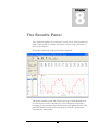
The Results Panel
65
Parameters Tab
67
Load Test Tab
71
Transient Tab
77
Lamination Geometry Tab
12
Materials Tab
16
CHAPTE R
Armature Winding Tab
18
The Field Explorer Panel
Mechanical Tab
21
Manual Excitation
82
Drive Circuit Tab
23
Existing Results
96
CHAPTE R
6
The Settings Panel
FE Solver & Mesh Control
34
35
User Defined Coefficients & Functions 36
Permanent Magnet Material
37
Steel Lamination Material
40
9
81
1
Chapter
About BLDC
BLDC is a brushless DC simulation environment. It is designed for quick learning, ease
of use, and the ability to provide powerful results. The goal of this software is to allow the
designer to experiment with such things as materials, geometries and winding
configurations, without ever having to build a prototype. The results provided by BLDC
are as good as test data but achievable in a much shorter time frame and at lower cost. As
you will see, BLDC provides parameterized results such as voltages, currents, torque and
power together with more esoteric results such as flux, iron loss and current density.
BLDC is divided into five distinct panels:
•
Settings Panel
This panel allows you to examine and adjust the material properties
of all magnetic materials loaded into the MagneForce suite of
simulators. Here you will find magnetic curves for both steel and
permanent magnet materials. You can also add new materials to the
MagneForce suite of simulators. This panel also contains global
software parameters that control such things as mesh density.
•
Design Panel
In this panel you will define the physical dimensions of the machine
as well as choose the armature and field materials plus define the
windings. Whenever you create or open a new or existing project,
you will first be placed at the design panel.
•
Run Panel
Once you have selected and described a machine, the run panel is
used to select the type of simulation plus initiate the simulation
process. Choices of simulation include parameter, load, fault study,
asymmetrical or special. Once a type is selected, you may then select
the number of load points, associated parameters and begin the
simulation.
1
•
Results Panel
Upon simulation completion, the performance results panel is used
to view the various parameterized output. Output ranges from the
open circuit machine parameters up to and including the complete set
of machine and load voltage and current waveforms, as well as
torque and power.
•
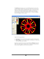
Field Explorer Panel
The field explorer panel is used to display the machine geometry,
finite element mesh, magnetic field density, current density and iron
loss density. These fields can be displayed for any of the load solution
points.
BLDC allows you to create a new project from a pre-defined list, modify the
project and then save it under a different name. In this way, you can work
with several design variations simultaneously. Projects can be opened and
saved at any time and the number of total projects is limited only to the size
of your hard disk drive.
2
2
Chapter
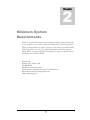
Minimum System
Requirements
BLDC is a powerful finite element based electromagnetic modeling software package, and
as such it performs a large amount of mathematical computations. The two largest factors
affecting system performance, in software of this type, are the processor speed and available
memory. Often times, users can gain a significant performance enhancement simply by
adding RAM. Accordingly, MagneForce recommends you equip your computer with the
maximum practical amount of RAM.
Pentium III
Windows NT, 2000 or XP
256 MB RAM
200 MB free hard drive space
SVGA monitor operating at 1024 X 768 resolution or
800 X 600 resolution if using small fonts
Mouse pointing device
3
3
Chapter
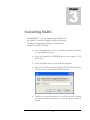
Installing BLDC
Installing BLDC is an easy multi-part procedure. First,
the software is installed. Secondly, the license.txt file must
be copied to the appropriate directory. And finally, the
hardware key must be attached.
•
Close all applications. It is best to perform the installation without
any other applications open.
•
Insert the MagneForce CD-ROM disk into your computer’s CDROM drive.
•
From the START menu, choose the RUN command
•
Type into the RUN command dialog box D:\SETUP.EXE, where
D: is the name of your computer’s hard disk drive.
•
Follow the onscreen instructions. You will be allowed to change
the software installation directory as well as the program folder, if
desired.
4
•
Depending upon your version of Windows, you may be instructed
to re-boot your computer and to re-run the installation routine.
Also some versions of Windows do not completely close the
installation DOS window. If this is the case, close the window
manually by clicking the X in the upper right hand corner.
•
After installation completion, copy the LICENSE.TXT file to the
C:\PROGRAM FILES\MAGNEFORCE subdirectory if you
accepted the default installation directory from step 4 above. If you
modified this directory structure, the LICENSE.TXT file must be
copied into the MAGNEFORCE directory, that is the directory
containing BLDC.EXE. The LICENSE.TXT file unlocks and
allows the appropriate simulators to run. If you do not have a
LICENSE.TXT file, please contact MagneForce.
•
Attach the security key, supplied with the software. The security
key will either be the parallel port variety or the USB variety. In the
case of the USB variety your computer will perform a brief
installation routine the first time that the key is inserted in each
USB port
•
Congratulations. Software installation is now complete.
5
4
Chapter
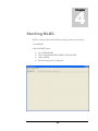
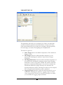
Starting BLDC
BLDC is written to follow normal Windows operating standards and conventions.
To start BLDC,
Click the START button
•
•
•
•
Go to PROGRAMS
Click on MAGNEFORCE SIMULATION SUITE
Click on BLDC
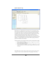
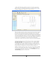
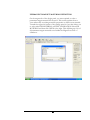
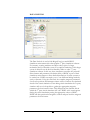
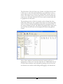
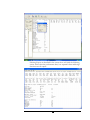
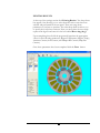
The following screen is displayed
6
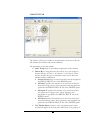
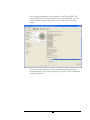
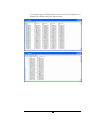
If this is the first time you have started BLDC or you have not saved any
projects, your only option will be to select NEW from the PANEL
TOOLBAR. Doing so will give you a list of default projects from which to
choose.
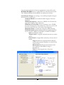
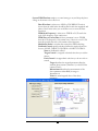
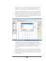
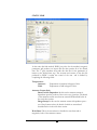
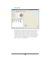
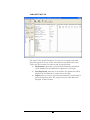
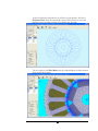
Choose a project that most closely resembles your desired project. Once a
choice has been made you will be prompted to save the project under a
new name. At this point you may choose to save the project to any folder
you wish. The default project location is C:\PROGRAM
FILES\MAGNEFORCE\BLDC\PROJECTS.
7
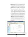
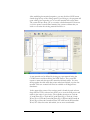
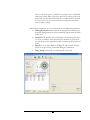
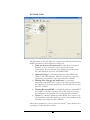
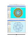
After Clicking SAVE, your newly named project will be opened and you
will be placed at the DESIGN panel.
8
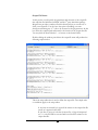
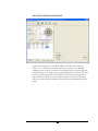
A listing of recently opened projects is available under the File menu. Click
FILE then scroll down the option list and highlight and click the desired
project.
9
10
5
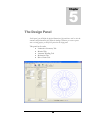
Chapter
The Design Panel
In this panel, you will define the physical dimensions of the machine as well as select the
armature and field materials plus define the windings. Whenever you create or open a
new or existing project, you will first be placed at the design panel.
This panel has five tabs:
• Lamination Geometry Tab.
• Material Tab.
• Armature Winding Tab.
• Mechanical Tab.
• Drive Circuit Tab.
11
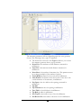
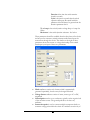
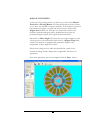
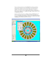
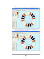
LAMINATION GEOMETRY TAB
This tab has sections on the left that describe the physical dimensions of
the field, armature and machine in general. On the right, is a cross
sectional drawing of the machine.
The field parameters will vary depending upon the exact rotor geometry
chosen. The following is for a type 613 permanent magnet rotor:
• The list button to the left of the Type field allows you to select
the rotor geometry from a pop up window.
• Outer Dia is the rotor outside diameter including magnets
measured in millimeters.
• Inner Dia is the diameter of the machine shaft measured in
millimeters.
• Num Poles allows you to select the number of poles of the
machine from the drop down list.
• Magnet Arc Style is set to 1 if the magnet arc is measured from
the rotor center or 2 if the arc is measured from the tip of the
magnet, if so enter arc value.
• Magnet Thk is the thickness of the permanent magnet material
measured in millimeters.
• Magnet Width is the width of each magnet piece in millimeters.
12
The armature parameters will vary depending upon the exact geometry
chosen. The following is for a type 703 armature:
• The list button to the left of the Type field allows you to select
the armature geometry from a pop up window.
• Outer Dia is the armature outside diameter, measured in
millimeters.
• Inner Dia is the armature inside diameter measured, in
millimeters.
• Num Slots is the number of armature slots. This parameter must
be an integer multiple of the number of phases.
• Tooth Width measured at the tooth stem in millimeters.
• Yoke Width is the distance from the bottom of the slot to the
outside diameter of the armature, in millimeters.
• Slot Open is the slot width at the opening, measured in
millimeters.
• Tip Def
• Tip Thickness at the slot opening in millimeters.
• Foot Thk foot back thickness in millimeters.
• Tip Rad tip radius in millimeters.
• Slot Top R corner radius at top of slot in millimeters.
• Slot Bottom R corner radius at bottom of slot in millimeters.
13
•
Slot Wedge Thk is used if slot wedges are used and is the
thickness from the inner diameter towards the outer diameter,
measured in millimeters.
The general machine parameters near the bottom of the screen are:
• Stack is the length of machine measured in millimeters.
• Skew is the machine skew end to end measured in slots.
• Weight is a calculated value of the rotor and stator lamination’s
weight in kilograms.
The program will calculate the machine air gap based upon your input
dimensions. If the resultant air gap is negative, it will be displayed in red.
Please note that when making large wholesale changes to the machine
dimensions, the graphical display may be left blank or seem distorted. This
is due to the fact that some geometry parameters have changed while
others have not yet been updated. Continue with your geometry change
inputs and the display will return to normal once all parameters have been
correctly updated.
14
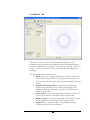
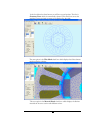
Under the drawing of the machine cross section is an APPLY and
CANCEL button. These buttons are used to apply or cancel changes in
the geometry figures from above. Next to these are four buttons for FIT
ALL, ZOOM IN, ZOOM OUT and MOVE. They can be used together
with the scroll bars to enlarge and inspect your geometry. When satisfied,
click the FIT ALL button to return the cross section to normal size.
The button MODIFY/DRAW button is used to launch ARBIDRAW
which is MagneForce’s stand alone drawing package that will allow you to
make major geometry changes to a slot module. Please see the ArbiDraw
user manual for further explanation.
After you are satisfied with your design, use the SAVE button on the panel
toolbar to commit your changes to disk.
15
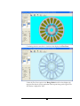
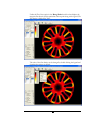
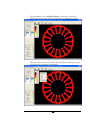
MATERIALS TAB
This tab has sections on the left that describe the attributes of the
permanent magnet material, steel laminations and other electromagnetic
materials as applicable to the design. On the right is a drawing of the cross
section of the rotor and below is an area that describes the damper bar
windings.
The permanent magnet parameters are:
• Grade is the type of magnet material that the field is made from,
select from the drop down list. If your particular material is not
listed you may add it using the settings panel described in the next
section.
• Magnetization Orientation describes how the permanent
magnets are magnetized. Choose radial if the magnetic field
emanates radially from the rotor or parallel if the field lines are
parallel to each other.
• Center Offset is active only when radial orientation is chosen. It
is the angle at which the field differs from straight radial.
• Relative Angle is active only when parallel orientation is chosen.
It is the angle that the field differs from straight parallel.
• Magnet Vol is a calculated value of the permanent magnet
volume measured in cubic millimeters.
16
The Lamination parameters are:
• Field Lam is the type of steel the field stack is constructed from,
please select from the drop down list.
• Armature Lam is the type of steel the armature stack is
constructed from, please select from the drop down list.
Please note that if your particular steel does not appear in the list you will
have a chance to add it utilizing the settings panel which will be explained
in the next section.
The damper bar parameters are:
• Bar Ohm Per Meter is the resistance of the bar material,
measured in ohms per meter.
• End Ring Ohm Per Meter is the resistance of the end ring
material, measured in ohms per meter.
• Bar R is a calculated parameter and is the actual machine bar
resistance in ohms.
• End Ring Rd is a calculated parameter and is the d-axis
resistance parameter of the end ring.
• End Ring Rq is a calculated parameter and is the q-axis
resistance parameter of the end ring.
• End Ring Full Connection should be checked if all bars are
connected to the end ring.
• Damper Winding Active should be checked if you would like
the simulation to proceed with the effects o
Under the drawing of the machine cross section is an APPLY and
CANCEL button. These buttons are used to apply or cancel changes in
the geometry figures from above. Next to these are four buttons for FIT
ALL, ZOOM IN, ZOOM OUT and MOVE. They can be used together
with the scroll bars to enlarge and inspect your geometry. When satisfied,
click the FIT ALL button to return the cross section to normal size.
After you are satisfied with your design, use the SAVE button on the panel
toolbar to commit your changes to disk.
17
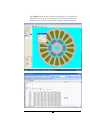
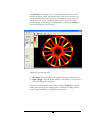
ARMATURE WINDING TAB
This tab describes the armature winding including wire size, numbers of turns,
and connection type. The tab has sections on the left that describe the
armature winding attributes. On the right, is a graphical representation of
the cross section of the rotor.
•
•
•
•
•
No of Phases is the number of phases of the armature
windings.
Connection can be either “Y” or Delta, choose from the drop
down list.
Branches is a parameter that describes how the coils are
connected to each other to form the winding. If they are
connected in series then branches are 1, if they are connected
in parallel then branches are 2 or higher. Simply put branches
is the number of parallel paths through a particular phase
winding.
Bi-Filer Wdgs can be set to either YES or NO, indicating
whether or not the drive circuit uses a b-filer design in which
there are no low side switches.
Insulation Thk is the thickness of the insulating material that
surrounds the interior of the slot in millimeters.
18
•
•
•
Wire Tension is the tension with which the coil is wound, this
tension can affect the resistance of the coil. A value of 1
indicates no deformation of the wire during winding.
Winding Type can be either set to standard or fractional,
select from the drop down list. A standard winding is one in
which full winding symmetry exists in each pair of poles. A
fractional winding is one in which full winding symmetry does
not exist in each pair of poles but does exist within each phase.
Wire Size-1 & Wire Size-2 is the gauge of the wire used to
wind the coils. Select these from the table by clicking the select
button to the left of the name. Also included in this table is the
Parallel Strands parameter. This parameter specifies the
number of parallel strands that the winding is composed of.
The reason there are two Wire Size parameters is so that a
winding may be composed of two wires of different sizes. The
actual existence of each size is specified in the winding table
below.
Based upon your input, several parameters are calculated
• Ra is the phase resistance as viewed from the machine’s
terminals.
• Min Slot Area is cross sectional area of the slot measured in
square millimeters.
• Max Slot Fill is the percentage fill of the fullest slot.
• Copper Weight is the weight in kg of the copper winding
specified in the winding table.
• Wdg Symmetry in Number of Poles is the symmetry if any
that exists in the winding as related to the number of poles.
This parameter can help spot an unintentionally unbalanced
winding and is used to determine how the machine is solved.
For example a 60 degree phase belt winding can be solved in
one pole while a 120 degree phase belt winding must be solved
in two poles.
The table below these parameters, together with the drawing to the right,
describe exactly how the coils are wound within the slots of the armature.
The table lists the coils (which are calculated based upon your input on the
lamination geometry tab) from beginning to end. To describe the winding,
fill in the columns CURRENT IN, CURRENT OUT, TPC and WIRE for
all coils.
•
•
CURRENT IN is the slot number, for this coil, in which current
would travel into the computer screen.
CURRENT OUT is the slot number, for this coil, in which
current would travel out from the computer screen.
19
•
•
TPC is the number of turns per coil. This is the physical number
of wires that belong to this coil, however be careful not to confuse
this with the number of strands. For instance a coil that is wound
with 5 strands in hand but only 2 turns per coil would have a TPC
setting of 2 and not 10.
WIRE can be set to SIZE 1, SIZE 2 or SIZE 1&2. Simply place
the cursor in the WIRE column on each line and click to toggle to
the correct setting. The actual size of the wire is specified above in
the WIRE SIZE tables.
Along the right hand side of the table are three tabs labeled PHASE A,
PHASE B and PHASE C. In the case of a standard winding the program
will complete the winding tables for PHASES B and C based upon your
input from PHASE A. In the case of a fractional winding you must click
each tab and complete the winding table for each phase individually.
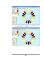
Just above the armature drawing are three check boxes for the three
phases of the machine. Checking each box will cause the corresponding
phases’ winding to be drawn. In this way one can often spot mistakes in
the winding table, by comparing winding symmetry among the phases.
Under the drawing of the machine cross section is an APPLY and
CANCEL button. These buttons are used to apply or cancel changes in
the geometry figures from above. Next to these are four buttons for FIT
ALL, ZOOM IN, ZOOM OUT and MOVE. They can be used together
with the scroll bars to enlarge and inspect your geometry. When satisfied,
click the FIT ALL button to return the cross section to normal size.
After you are satisfied with your design, use the SAVE button on the panel
toolbar to commit your changes to disk.
20
MECHANICAL TAB
This tab allows you to enter mechanical parameters that describe the
machine’s mechanical properties. The active parameters are:
• Fan Power Coeff is a parameter that describes the wattage
absorbed by the machine’s fan in Watts per cubic rpm.
• Stator HF Loss Coef estimated high frequency eddy current loss
in stator, in Watts per cubic rpm
• Rotor HF Loss Coef estimated high frequency eddy current loss
in rotor, in Watts per cubic rpm
• Thermal Model drop down box to select external user defined
thermal model (not yet implemented)
• Rotor M. I. is the calculated rotational moment of inertia of the
rotor.
• Additional M. I. is any additional moment of inertia that you
would like to add such as a fan or the load.
• Total M. I. is the sum of the above rotational and additional
moments of inertia.
• Gearing Efficiency is the efficiency of any gearing attached to the
motor in per unit.
• Viscous Torque Loss is any mechanical torque loss in the above
gearing.
21
In the lower right corner is an APPLY and CANCEL button. These
buttons are used to apply or cancel changes in the mechanical parameters
from above. After you are satisfied with your design, use the SAVE button on
the panel toolbar to commit your changes to disk.
22
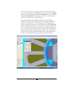
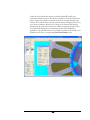
DRIVE CIRCUIT TAB
Within this tab you will describe the schematic layout of the machine’s drive
circuit. The tab is divided into two major sections, the schematic drawing area
to the right and a column to the left used for parameter settings and switch
visualization. The operation of the drawing section is similar to many popular
schematic drawing and capture packages. Using the drawing aids and
component buttons along the top of the schematic area you can, quickly &
easily, construct Brushless DC drive circuits ranging from simple rotor position
feedback to complex PWM control. The drive circuit topology will then be
used in the simulation of the machine.
The upper portion of the left hand column contains several parameter settings.
• Inverter Advanced Firing is the amount, in degrees, that you wish to
advance fire the inverter switches.
• Inverter Switch Dead Angle is the amount, in degrees, that you wish
to reserve between one inverter switch turning off and the next switch
turning on.
The middle portion of this column contains several symmetry settings. These
settings are used to conserve simulation time. The program will use these
23
settings in determining exactly how much of the machine and how much of
the complete AC cycle it needs to simulate.
• Phase to Phase can be checked if the machine exhibits drive phase to
phase symmetry.
• Bi-Polar can be checked if the drive circuit exhibits Bi-Polar
symmetry.
The lower portion of this column is a graphical representation of the switch
on-off sequence versus electrical degrees. In simple rotor position feedback
control this area can provide a quick visual confirmation that you have set all
of the switch on-off attributes correctly.
Beginning with a blank screen you may select any of the buttons above the
schematic drawing area. Select the button you wish by rolling your mouse
cursor over the item and clicking the left mouse button. Next move the mouse
cursor into the schematic drawing area and place by clicking the left mouse
button again. The selected item will now appear on the schematic drawing
area. Depending upon the item selected access the item’s attributes by rightclicking the item on the drawing area and selecting attributes. Each item has
attributes that are appropriate to itself. Additionally, right clicking an item will
allow you to rotate, flip, delete, copy and or paste the item. These options are
available to the appropriate items.
24
•
•
•
Armature will place an armature of the type that was selected on the
armature winding tab previously. For example if a 3-phase Y
connected winding was selected on the armature tab you will see a
schematic of this exact armature with access to the following leads A,
B, C and N. There are no attributes available for the armature item.
Excitation will place one of three voltage sources onto the schematic
drawing area. When initially selecting excitation you will be presented
with 3 additional choices, V source, AC Bridge and DC Excitation.
Choosing V source will place a simple ideal voltage source while
choosing AC Bridge will place a standard AC bridge rectifier voltage
source and choosing DC Excitation will place a standard voltage
source in series with a resistor, onto the drawing area. The attributes of
the actual voltage source in each of these excitation models can be
accessed by right clicking the source itself. Attribute options are AC or
DC, voltage magnitude and frequency if AC is selected. Additionally,
you can rotate or scale the objects size from this pop-up window as
well. The other items such as resistors and diodes contained in the AC
Bridge and DC Excitation models also have attributes that may be
displayed by right clicking the actual device.
Inverter will place onto the drawing area a standard drive circuit
inverter based upon the exact armature selected on the armature tab
previously. This inverter will be composed of the appropriate number
of switches and diodes connected in a manner suitable to drive the
selected armature. Each individual component in this preconfigured
inverter is selectable and its attributes modifiable by right clicking the
component itself.
25
Once the above three major components are placed onto the schematic
drawing surface any additional components such as filter capacitors or
inductors, shut resistors, extra switches or diodes may be placed onto the
drawing surface. Each individual component will have a specific set of
attributes, detailed below, available for setting and accessed by right clicking the
component itself. Each component’s attribute box will allow the component
to be scaled in size or rotated on the page.
•
•
•
•
Resistor attributes include name and resistance. The resistor name is
automatically generated sequentially, however it may be changed if
desired and the resistance value is set in Ohms.
Inductor attributes include name and inductance. The inductor name
is automatically generated sequentially, however it may be changed if
desired and the inductance value is set in Henrys.
Capacitor attributes include name and capacitance. The capacitor
name is automatically generated sequentially, however it may be
changed if desired and the capacitance value is set in Farads.
Switch attributes include name, control, and a junction resistance
model.
Name the switch name is automatically generated
sequentially, however it may be changed if desired.
Control
Rotor Ang
Phase Ang in simple rotor position feedback
control, the degree at which the switch will
turn on.
Algorithm can be set to one of 4 different
choices, which determines simple rotor
position feedback (local square voltage) or
one of 3 different PWM control schemes
which are described in more detail in the next
section.
On Band Width amount of time the switch
will remain on, in degrees
Time the switch operates for a predetermined time as
described by the following parameters.
Delay the delay, in seconds, if any, before the
switch starts operating.
Algorithm Pulse-Local used to pulse the
switch according to the following parameters
or Time Local used to control the switch
according to time.
Frequency the frequency of the pulse
Duty Cycle in per unit, the ratio of the on to
off time of the switch
26
Duration is the time the switch remains
closed in seconds.
Cycle is the time in seconds that the whole
operation will repeat. Be careful with this
parameter it should always be greater than the
duration parameter above.
Vj at 1 amp is the switch junction voltage drop at 1 amp. See
below.
Resistance is the switch junction resistance. See below.
These parameters should be available from the data sheet of the device
and are used to construct a switch resistance model based upon the
current flow through the device. The window to the right of these
parameters shows the current vs voltage relationship of this switch
based upon your input of these two parameters.
•
•
•
•
Diode attributes consist only of name which is automatically
generated sequentially, however may be changed if desired.
Voltage Source attributes consist of name, source type AC or DC,
magnitude
Ground point must be set as a reference, typically on the negative lead
of the excitation source. The ground point does not have any
attributes.
Intersection point is used to connect multiple component leads to a
common voltage point within the circuit. It’s attributes consist only of
27
•
•
name which is automatically generated sequentially, however may be
changed if desired.
Ammeter can be placed anywhere within the circuit in which you
would like to know the current. Upon simulation the results of this
meter will appear in the results portion of the program. It’s attributes
consist only of name which is automatically generated sequentially,
however may be changed if desired.
Voltmeter can be placed across any portion of the circuit in which
you would like to know the voltage. Upon simulation the results of
this meter will appear in the results portion of the program. It’s
attributes consist only of name which is automatically generated
sequentially, however may be changed if desired.
Once all appropriate components have been placed upon the schematic
drawing area you may connect them to form the desired drive circuit. To
connect components roll your cursor over the device endpoint until a red
circle appears. At this point left click and drag to the next component. Please
note that as soon as you left click the first component the cursor will change to
28
a hand symbol and remain until the connection to the other component is
made. You may move individual components or connection lines by simply
clicking and dragging the component to its desired location.
When all suitable connections and movements have been made select Apply at
the bottom of the drawing area and your circuit will be saved. At any time
before you click Apply you can click Cancel and all changes in the drawing area
since the last Apply will be erased. To the left of the Apply and Cancel buttons
are the Select all and Clear All buttons. Use the Select All button to highlight all
components on the drawing area. You may then click and drag all the
components as a group. The Clear All button will clear the entire drawing area.
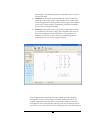
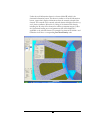
In the upper right hand corner of the drawing area there is a button labeled
ROTOR ANG PWM. This button allows access to the 3 different PWM
control schemes that are part of BLDC. The button is normally graded out
until a PWM control scheme is selected in the attributes of at least one of the
inverter switches. It is important to note that all switches should be set
similarly, it would not make any sense to have some of the switches operating
under one control scheme while others are following a different scheme. To
set each switch, double click it and select one of the SYSTEM modes in the
ALGORITHM parameter as shown below.
29
30
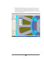
Once all system switches have been set appropriately you may click on the
ROTOR ANG PWM button to further define the selected control scheme.
The 3 different PWM modes that BLDC can simulate are as follows:
System Square Voltage uses a strategy to try and keep the phase voltage to
the motor to be a square wave.
Conduction Band is the conduction band in degrees of the base
waveform
PWM Style Frequency is either set to FIXED or Fc/Fb and is the
style of the frequency of the carrier wave.
PWM Freq or Carrier/Base if above parameter is set to FIXED
then this is the frequency of the carrier wave, if above is set to Fc/Fb
then this specifies the ratio of the carrier to base frequency.
Modulation Index is an index that controls the PWM switching
Feedback Control specifies whether feedback is employed and can
be set to NONE, TARGET-CONTROL or LIMIT-CONTROL.
None no feedback is utilized
Target Control is a targeted or desired value that you wish to
achieve
Limit Control is an upper limit value that you do not wish to
exceed.
Target describes the targeted parameter either the
armature phase current (Armature A) or the DC Bus
current (I am11)
Measurement describes the measurement of the
above parameter either RMS, Average or
Instantaneous.
Value the actual targeted value of the above
parameter.
31
System PWM Freeform employs a control strategy to try and keep the phase
voltage to the motor to be a sine wave.
Base Waveform is either set to SINE or FOURIER. If Fourier is
chosen then the table below should be filled in with the magnitude and
phase of the Fourier series you would like to use to create the Base
waveform.
PWM Style Frequency is either set to FIXED or Fc/Fb and is the
style of the frequency of the carrier wave.
PWM Freq or Carrier/Base if above parameter is set to FIXED
then this is the frequency of the carrier wave, if above is set to Fc/Fb
then this specifies the ratio of the carrier to base frequency.
Modulation Index is an index that controls the PWM switching
Feedback Control specifies whether feedback is employed and can
be set to NONE, TARGET-CONTROL or LIMIT-CONTROL.
None no feedback is utilized
Target Control is a targeted or desired value that you wish to
achieve
Limit Control is an upper limit value that you do not wish to
exceed.
Target describes the targeted parameter either the
armature phase current (Armature A) or the DC Bus
current (I am11)
Measurement describes the measurement of the
above parameter either RMS, Average or
Instantaneous.
Value the actual targeted value of the above
parameter.
32
System Bang-Bang Current employs a control strategy to try and keep the
motor phase current as close to a specified waveform (sine, trapezoidal or
square) as possible.
Base Waveform is either set to SINE, TRAPEZOID, SQUARE or
FOURIER. If Fourier is chosen then the table below should be filled
in with the magnitude and phase of the Fourier series you would like
to use to create the Base waveform.
Conduction Band active only for the Trapezoid or Square wave
options and is the width of the base wave
Peak Value is the maximum of the phase current that we are trying to
control.
Tolerance is the tolerance around the above peak value that the
control scheme will operate around.
33
6
Chapter
The Settings Panel
This panel allows you to examine and adjust the material properties of all magnetic
materials loaded into the MagneForce suite of simulators. Here you will find magnetic
curves for both steel and permanent magnet materials. This panel also contains global
software parameters that control such things as mesh density.
When first selected the settings panel will be displayed as:
34
FINITE ELEMENT SOLVER & MESH CONTROL
PARAMETERS
On the right side of this panel are several parameters that apply globally to
the solver and to the generation of the finite element mesh. The default
button can be used to restore these parameters to their original values.
• Min Distance is the minimum distance that will be allowed
between two nodes. This value should not normally need to be
adjusted.
• Rot. Mesh Density is a factor that controls the density of the
rotor mesh. A value of 1 indicates a “normal” mesh density.
Decreasing this parameter will cause the mesh density to decrease,
while increasing it will cause the mesh density to increase.
• Sta. Mesh Density is a factor that controls the density of the
stator mesh. A value of 1 indicates a “normal” mesh density.
Decreasing this parameter will cause the mesh density to decrease,
while increasing it will cause the mesh density to increase.
• Forced Air Gap Layers determines the number of node layers
that will be forced within the airgap. A value of -1 indicates that no
forcing of layers will be done. This setting allows the program to
determine the number of air gap layers. Values of 0, 1 or 2 indicate
this specific number of layers of nodes will be forced.
• 3D Field Correction is parameter that corrects for 3D effects. If
your machine is heavily saturated you can choose to add up to 10%
flux linkage & inductance due to the end effects with this
parameter.
• Order of Elements can be set to either 1 or 2 to use first or
second order finite elements. Please note that cogging torque
calculations always use second order elements.
35
USER DEFINED COEFFICIENTS & FUNCTIONS
Under the solver and mesh control parameters are several settings that
allow the user to describe end-turn effects and to invoke an iron loss
model and/or a permanent magnet overhang model. The default button
can be used to restore these parameters to their original values.
• Fld Wdg ET Permeance is a coefficient that describes the
permeance of the end-turn winding of the field.
• Arm Wdg ET Permeance is a coefficient that describes the
permeance of the end-turn winding of the armature.
• Iron Loss Model is currently not implemented within BLDC.
• Magnet Overhang Coeff is currently not implemented within
BLDC.
36
PERMANENT MAGNET MATERIAL DEFINITION
On the magnet tab of the design panel, you were required to select a
permanent magnet material for the rotor. This section explains how to
view and modify an existing material’s properties or define a new material.
Towards the upper left corner of the settings panel is a box that allows you
to select either PM MATERIAL or STEEL LAMINATION. Select PM
MATERIAL and then click OPEN to the right. This will bring up a list of
all permanent magnet materials saved within the MagneForce suite of
simulators.
37
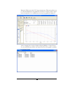
Select a material from the list and click OPEN.
This screen displays in tabular and graphical form several B-H curves for
the selected permanent magnet material. Each curve is at a different
temperature. The name of the selected material appears above the upper
table which is the B-H curve at 20 degrees Celsius. The lower table is the
temperature coefficient table which describes how the B-H curve changes
with increasing temperature. The columns in this table (C-M and C-H) are
temperature coefficients that are simply multiplied by the B-H values at 20
degrees Celsius. Doing so yields the successive curves in the graph at the
right. You will notice that the number of curves in the graph equals the
number of tabular entries in the temperature coefficient table.
Additionally, as you highlight an entry in this table, the corresponding
curve is accentuated.
The values in the two tables can be adjusted and the results reflected in the
curves to the right. Simply click on an entry and change it. The table will
be immediately sorted and the graph updated. Additional data points can
be added by using the scroll bars to position the cursor at the end of the
table. Simply enter your new values and the graph and table will again be
immediately updated.
38
The viewable size of the two tables and the graph area can be changed.
Simply position your cursor on the area between either the tables or
between a table and the graph area and click and drag to the desired size.
After modifying the material properties, you may click the SAVE button
along the top of the settings panel. Upon doing so, the program will open
a dialog box requesting you to save the material with a new name. The
system will not allow you to over-write a default material. If however you
have opened a user defined material the system confirms that you wish to
over-write the existing material and does so.
A new material can be defined by closing any open material, using the
CLOSE button and then clicking the NEW button. The system will
request a name and then open the material with blank tables. You can then
populate the tables with data points and when finished save the new
material. This new material will now be available to all MagneForce
Simulators.
In the upper right corner of the settings panel is the units selector drop
down box. This selector box allows you to view the B-H curves and tables
in the units of your choice. The available selections are Tesla & A/m or
Gauss & Oersted or KGauss & KOersted. Select the units you are most
comfortable with.
39
STEEL LAMINATION MATERIAL DEFINITION
Similar to the permanent magnet material, BLDC provides for the
characterization of different steel materials. On the settings panel in the
upper left corner, click STEEL LAMINATION, then to the right click
OPEN. A dialog box will appear requesting you to select a steel material
from a list of all materials saved within the MagneForce suite of
simulators.
40
Select a material and click OPEN.
Similar to the permanent magnet material, the B-H curve for the steel
material is displayed in both tabular and graphical format. The name of the
selected material appears just above the B-H tabular values, while a graph
of these points appears to the right.
The values in the table can be adjusted and the results reflected in the
curve to the right. Simply click on an entry and change it. The table will be
immediately sorted and the graph updated. Additional data points can be
added by using the scroll bars to position the cursor at the end of the
table. Simply enter your new values and the graph and table will again be
immediately updated.
The viewable size of the table and the graph area can be changed. Simply
position your cursor on the area between the table and the graph area and
click and drag to the desired size.
41
After modifying the material properties, you may click the SAVE button
found along the top of the settings panel. Upon doing so, the program will
open a dialog box requesting you to save the material with a new name.
The system will not allow you to over-write a default material. If however
you have opened a user defined material, the system confirms that you
wish to over-write the existing material and does so.
A new material can be defined by closing any open material using the
CLOSE button and then clicking the NEW button. The system will
request a name and then open the material with blank tables. You may
then populate the table with data points and when finished, save the new
material. This new material will now be available to all MagneForce
Simulators.
In the upper right corner of the settings panel is found the units selector
drop down box. This selector box allows you to view the B-H curves and
tables in the units of your choice. The available selections are Tesla &
A/m & Watts/Kg or Tesla & KA/m & Watts/Kg or Tesla & A/m &
Watts/Lb or Gauss & Oersted & Watts/Kg or KGauss & KOersted &
Watts/Kg or Gauss & Oersted & Watts/Lb or KGauss & KOersted &
Watts/Lb . Select the units with which you are most comfortable.
42
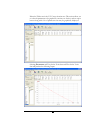
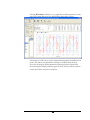
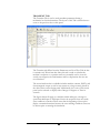
With STEEL LAMINATION still selected, click the IRON LOSS button.
A series of loss curves in Watts/Kg/Hz is displayed in both graphical and
tabular format. Each of the curves is at a certain frequency. The table to
the left indicates the frequency at which these losses have been
determined. Each curve is represented by the pair of columns titled B and
W with the same Frequency entry n. Use the scroll bars to see the table in
its entirety. The values in the table can be adjusted and the results reflected
in the curve to the right. Simply click on an entry and change it. The table
will be immediately sorted and the graph updated. Additional data points
can be added by using the scroll bars to position the cursor at the end of
or to the right of the table. Simply enter your new values and the graphs
and table will again be immediately updated.Additionally, the viewable size
of the table and the graph area can be changed. Simply position your
cursor on the area between the table and the graph area and click and drag
to the desired size.
As with the B-H curve the units of the loss curves can be changed. In the
upper right corner of the settings panel select from the drop down list the
units you are most comfortable with. The available selections are Tesla &
A/m & Watts/Kg or Tesla & KA/m & Watts/Kg or Tesla & A/m &
Watts/Lb or Gauss & Oersted & Watts/Kg or KGauss & KOersted &
Watts/Kg or Gauss & Oersted & Watts/Lb or KGauss & KOersted &
Watts/Lb .
43
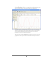
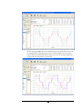
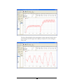
With STEEL LAMINATION and IRON LOSS still selected, click the
LOSS MODEL button.
Two additional graphs and one table will appear on your screen. The
graphs are the LOSS MODEL CURVES which plots Loss versus
Frequency, and the K & Y PARAMETERS CURVES which plots K & Y
versus Flux Density. The loss model curves are best fit curves to the
associated data points which is the loss expressed in Watts/Kg/Hz vs Hz
for a given flux density. The slope and Y intercept of these best fit curves
are then the K and Y parameters to the left, which are plotted vs the peak
flux density from a sinusoidal excitation. This loss model is used in the
program’s iron loss calculation. The table to the left contains the data
points for the K & Y Parameters. The values in the table can be adjusted
and the results reflected in the curves to the right. Simply click on an entry
and change it. The table will be immediately sorted and the graph updated.
Additional data points can be added by using the scroll bars to position the
cursor at the end of the table. Simply enter your new values and the graph
and table will again be immediately updated.
The viewable size of the table and the two graphs can be changed. Simply
position your cursor on the area between either the table and the graphs or
between the two graphs and click and drag to the desired size.
44
After modifying the material properties you may click the SAVE button
along the top of the settings panel. Upon doing so the program will open a
dialog box requesting you to save the material with a new name. The
system will not allow you to over-write a default material. If however you
have opened a user defined material, the system confirms that you wish to
over-write the existing material and does so.
In the upper right corner of the settings panel is the units selector drop
down box. This selector box allows you to view the B-H curves and tables
in the units of your choice. The available selections are Tesla & A/m &
Watts/Kg or Tesla & KA/m & Watts/Kg or Tesla & A/m & Watts/Lb
or Gauss & Oersted & Watts/Kg or KGauss & KOersted & Watts/Kg or
Gauss & Oersted & Watts/Lb or KGauss & KOersted & Watts/Lb .
Select the units with which you are most comfortable.
45
7
Chapter
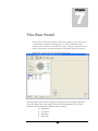
The Run Panel
Once you have selected and described a machine, the run panel is used to select the type
of simulation plus initiate the simulation process. Choices of simulation include
parameter, load, transient, or data link. Once a type is selected, you may then select the
number of data points, associated load parameters and finally begin the simulation.
When first selected the run panel will be displayed
The run panel has four tabs to the left, a message area to the upper right and a
check box field to the lower right. The tabs each correspond to a test of the
machine under certain load conditions they are titled:
• Parameters.
• Load Test.
• Transient.
• Data Link.
46
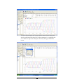
PARAMETERS TAB
The parameters tab can be set to calculate one of three very important
operational machine parameters described below. In many cases these
open circuit parameters can go along way to helping a designer quantify
his/her design, even before investigating the load parameters.
The tab has a space for
• Amb. Temp which is the ambient temperature of the machine in
degrees Celsius.
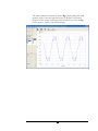
• OC Voltage check box which should be checked if you are
interested in obtaining the machine’s Open Circuit Voltages
Waveform.
• OC Wdg Inductances check box which should be checked if you
are interested in obtaining the machine’s Open Circuit Winding
Inductances versus rotor position. BLDC can calculate either the
apparent or incremental inductances. If you wish to calculate the
incremental inductances simply check the box otherwise the
apparent inductances will be calculated. In either case the complete
set of self and mutual inductances will be calculated.
• Cogging Torque check box which should be checked if you are
interested in obtaining the machine’s cogging torque waveform
versus rotor position. In the box enter the slot range over which
you would like the cogging torque calculated.
47
•
•
Total Pts drop down box which sets the number of data points
that the simulation will run for.
Wdg. Temp field is not active on this tab.
Underneath this area is where the individual parameters are set for each
load point. For the open circuit voltage and winding inductance test you
will supply the following:
• RPM is the speed of the machine in revolutions per minute.
• Hz is the frequency of the machine in Hertz. This is a calculated
value based upon the number of poles and the rpm.
• T_fld is the temperature of the field winding in Celsius.
• T_arm is the temperature of the armature winding in Celsius.
Below this area is a drop down box that specifies the finite element rotor
positions per slot pitch. This parameter is used to take advantage of
machine symmetry so that the number of finite element calculations can
be kept to a minimum and thus decrease simulation time. To the right is a
TOL CONTROL button that allows certain solution tolerances and
simulation starting points to be changed. The default values for these
parameters should work in almost all cases, therefore we do not
recommend changing these values unless directed to by MagneForce
technical support. To the right are the APPLY and CANCEL buttons that
allow you to commit or abandon your changes.
48
LOAD TEST TAB
The load test tab layout is similar to the parameters tab, however this tab
will simulate the machine under load conditions.
The parameters on this tab include:
• Amb. Temp which is the ambient temperature of the machine
• Driven By is a drop down box that can be set to one 4 choices,
Inverter Circuit, AC Sine V, AC Square V or AC Sine A. These
choices describe the type of excitation source used to drive the
machine under consideration.
• Inverter Circuit refers to the inverter drive circuit designed in
the DRIVE CIRCUIT tab of the DESIGN panel.
• AC Sine V specifies the machine to be run from an ideal AC
sinusoidal voltage source, whose frequency and magnitude are
specified in the DRIVE CIRCUIT tab of the DESIGN panel.
• AC Square V specifies the machine to be run from an ideal
AC square wave voltage source, whose frequency and
magnitude are specified in the DRIVE CIRCUIT tab of the
DESIGN panel.
• AC Sine A specifies the machine to be run from an ideal AC
sinusoidal current source, whose frequency and magnitude are
specified in the DRIVE CIRCUIT tab of the DESIGN panel.
• Use Tabular Input contains a series of parameters that when
checked will appear in the load point table below. The purpose of
49
this is to allow the user to override the settings of these individual
parameters on the Drive Circuit tab and use the values in the load
point table for each individual load. For example with Vs checked
it is very easy to set up a load run with several points that differ
only in supply voltage.
Below these parameters are several check boxes for additional parameters.
• Demag Prediction when checked the program will calculate any
potential demagnetization of the permanent magnet material while
under load.
• Load Pts field specifies the total number of load data points that
you wish to simulate. After specifying the number of points here
you will be given the opportunity later to further specify each load
point.
• Specify is set to either RPM or TORQUE and controls whether
speed or torque is being controlled during the simulation.
• Wdg. Temp is currently not implemented on this tab.
50
Below these parameters is the area where you further describe the load
points selected above. Depending upon the selections from above the
table may contain the following fields.
• RPM is the speed of the machine in revolutions per minute.
• Hz is the frequency of the machine calculated from the entry of
the above RPM value.
• Ckt Vs is the source voltage of the DC supply, remember this
value will override the value set on the Drive Circuit Tab.
• T_fld is the temperature of the field winding, in degrees Celsius.
• T_arm is the temperature of the armature winding, in degrees
Celsius.
Below this area is a drop down box that specifies the Finite Element (FE)
Rotor Positions Per Slot Pitch. This parameter is used to take advantage of
machine symmetry so that the number of finite element calculations can
be kept to a minimum and thus decrease simulation time. To the right is a
TOL CONTROL button that allows certain solution tolerances and
simulation starting points to be changed. The default values for these
parameters should work in almost all cases, therefore we do not
recommend changing these values unless directed to by MagneForce
technical support. To the right are the APPLY and CANCEL buttons that
allow you to commit or abandon your changes.
51
TRANSIENT TAB
The transient tab is similar to the load test tab in that it simulates machine
performance under load however it uses a time stepping solution method
that is capable of accurately calculating transient machine performance.
The solution technique used here will allow accurate calculation of the
actual machine parameters both during and after the transient has
occurred. This simulation will require more solution time therefore it is
not recommended for solution of a machine operating simply under steady
state conditions.
The parameters on this tab include:
• Amb. Temp which is the ambient temperature of the machine.
• End Time is the ending time of the simulation, in seconds. Be
sure to set this point an adequate amount beyond the Start Time of
the last load in the load point table below
• Max Step Size is the maximum width, in seconds, of the time
interval used during the simulation.
• Display Progress Every N Steps is a parameter used to control
how often data points are output to the screen when monitoring
the solution progress.
• Rotor Cycles for Steady State Calc specifies the number of AC
cycles at the end of each load point from which the steady state
parameters for that load point will calculated. For instance, setting
this parameter to 2 will result in the data from the last 2 AC cycles
52
•
of each load point being used to calculate the steady state
performance for each load point being studied.
Demag Prediction not available on the Transient Tab.
Below these parameters are several boxes for additional parameters.
• Total Steps is the number of total events or transitions from one
operating point to another during a solution.
• Specify is set to either RPM or TORQUE and controls whether
speed or torque is being given during the simulation.
• Wdg. Temp is currently not implemented on this tab.
Below these parameters is the area where you further describe the
operating points selected above. All operating points will require the
following parameters:
• Start Time is the time, in seconds, at which the operating point
will take effect. Note this point should be before the end time as
specified above.
• RPM is the speed of the machine in revolutions per minute.
• AF Angle is the advanced firing angle used during the simulation.
This parameter will override the setting on the Drive Circuit tab of
the DESIGN panel.
• T_fld is the temperature of the field winding, in degrees Celsius.
• T_arm is the temperature of the armature winding, in degrees
Celsius.
Below this area is a field labeled
• INITIAL RPM & Rotor Ang Deg are the initial speed and
rotor angle of the machine. This parameter is simply a starting
point, and used only when TORQUE is the given parameter, as
the speed will vary depending upon the operating point conditions.
To the right is a TOL CONTROL button that allows certain solution
tolerances and simulation starting points to be changed. The default values
for these parameters should work in almost all cases, therefore we do not
recommend changing these values unless directed to by MagneForce
technical support. To the right are the APPLY and CANCEL buttons
which allow you to commit or abandon your changes.
53
DATA LINK TAB
The Data Link tab is used to link MagneForce’s powerful BLDC
simulation environment with other popular 3rd party simulation software.
For instance, rotating machines are almost always part of a larger
mechanical and/or electrical system. If a complete simulation of this larger
system is desired it can be done in Simulink, Sabre or other 3rd party
simulation software. In this way these simulators can utilize the powerful
finite element and parameter calculation ability of BLDC as part of their
simulation environment to allow detailed simulations of entire systems to
be carried out. BLDC can employ one of two different linking methods,
static or dynamic. Using the static link, the complete magnetic parameters
for all rotor positions and armature current values of interest are calculated
ahead of the circuit simulation. Then during circuit simulation the 3rd party
simulator will use a lookup table to gather the appropriate magnetic
parameters for that instant in time. This differs from the dynamic link in
which the 3rd party circuit simulator will “call” BLDC at the certain points
during the circuit simulation passing the appropriate values to BLDC.
BLDC will then perform the magnetic solution and pass back the magnetic
parameters for that instant.
54
STATIC LINK
In the static data link method, BLDC pre-solves for the machine’s magnetic
parameters and produces an output data file that contains all of the desired
data. The 3rd party simulator then reads this data file for the parameters of
interest at the desired time step. The structure and content of the data file
produced by BLDC is under the control of the user and is defined by
completing the following fields:
Temperatures:
Armature:
Field:
Temperature of armature in degrees Celsius
Temperature of field in degrees Celsius
Armature Current Style:
Rotor Position Dependant: In this case the armature current is
dependent upon the position of the rotor at any given time. The details
of the armature current waveform are entered and described below in
the work sheet section.
Range Sweep: In this case the armature current is dependent upon a
set of fixed current values, the details of which are entered and
described below in the work sheet section.
Work Sheet: This is the area where we describe the waveform and or
magnitude/value of the armature current.
55
Style: Used in the Rotor Position Dependant case to describe the
waveform of the armature current, choices are:
None: Select when you wish to use the flux from the PM
materials only and to ignore any armature reaction.
Sinusoidal: Select when you wish to simulate using a
sinusoidal armature current waveform in addition to the PM
generated flux.
Square: Select when you wish to simulate using a square wave
armature current waveform in addition to the PM generated
flux.
Ref Frame: Specifies the frame of reference that the calculations and
data file will be produced in. Options are:
ABC: refers to the normal time domain ABC reference frame.
Multiple values can be entered, separated by a comma, so that
BLDC will calculate the magnetic parameters at each of the
specified current values. With this selection you will be
required to enter the following:
Ia pk (A): peak value of phase A current
Ia Ea (deg): angle between the A phase current and
resultant MMF.
DQ-1: refers to the popular dq reference frame in which
much control work is done. Multiple values can be entered,
separated by a comma, so that BLDC will calculate the
magnetic parameters at each of the specified current values.
Id (A): magnitude of q-axis current
Iq (A): magnitude of d-axis current
DQ-2: refers also to the dq refrence frame. Again multiple
values can be entered, separated by a comma, so that BLDC
will calculate the magnetic parameters at each of the specified
current values. However with this selection you will describe
the armature current by specifying the magnitude and phase of
Is, the resultant vector formed by Id & Iq:
Is (A): magnitude of Is
Is Er (deg): angle of Is
After setting the above parameters be sure to click the button titled CLEAR
TABLE and then click ADD TO TABLE. This will clear and then populate
the armature current table below with the appropriate values from the above
inputs. BLDC will populate the table with each combination of the above
parameters. For example the figures below show 2 values entered for the
magnitude of Ia and 2 values entered for the Ea angle. This will produce 4 lines
in the table since each magnitude needs to be paired with each angle. This table
can be thought of as the load point table from the parameter or load test tab.
When the static link is executed BLDC will sequentially calculate the output
data file using each of these 4 table entries as an input. In this way the output
56
file will consist of 4 distinct sections of output corresponding to each one of
these inputs.
57
Output File Name:
In this section you will specify the parameters and structure of the output file
that will form the link between BLDC and the 3rd party simulation package.
MagneForce provides a number of built in functions that you can choose to
form your output file. You also have the option of building your own
functions and writing any “C” code to be executed as the program runs. In this
box fill in the complete path and name for the location of the output data file.
You may click the button labeled … to browse to the desired folder.
Double clicking the window pane below the output file name will produce the
following script window.
This is the script editor that is used to define the output file. Two simple rules
or conditions apply to the script editor:
1. Any line not encased by $ signs will be written to the output data file
exactly as it appears in this table.
2. Any line or group of code that is encased by a $ sign is interpreted
as C++ code and will be executed and its result will be written to the
output data file.
58
There are two methods to include results in the output data file. First
MagneForce supplies many different functions for the most commonly
exported parameters. These can be accessed by clicking the FUNC MATLAB
or FUNC SPICE buttons located at the top of the window. The HELP button
will give detailed explanations of each of the parameters in a given function as
well as a sample of its correct usage. The second way to include results into
the output data file is for the user to write his/her own C++ code encased
again by the $ sign. Upon running the simulation the C code will be executed
and the results written to the output file. This option will only be necessary if
the desired parameter is not already included in one of the predefined
MagneForce functions.
Upon successful completion of the script editor click the OK button and then
click the EXECUTE button to run the actual simulation. A sample of the top
half and bottom half of the output data file for the above data link example
appears as the next two figures below. Notice how the lines not encased in the
$ sign have been explicitly written to the data file while code between the $
signs has been executed and the results written to the file. Also note the
corresponding section for each of the 4 distinct armature current runs.
59
The above file is now ready to be accessed by the 3rd party simulator.
60
DYNAMIC LINK
The parameters on this tab define the variables that will be passed between
BLDC and whatever other simulator is employed:
• Field and Armature Temperatures is either set to Constant or
Dynamic. If set to constant you must specify the actual
temperatures. If set to dynamic this parameter is passed in from
the other simulator for use by and within BLDC.
• Apparent Energy is a calculated parameter within BLDC and
output to the other simulator. Select the check box to cause this
parameter to be included in the output data files of BLDC.
• Winding Flux Linkage and Inductance is a calculated
parameter within BLDC and output to the other simulator. Select
the check box to cause this parameter to be included in the output
data files of BLDC.
• Winding Rotational EMF is a calculated parameter within BLDC
and output to the other simulator. Select the check box to cause
this parameter to be included in the output data files of BLDC.
• Torque is a calculated parameter within BLDC and output to the
other simulator. Select the check box to cause this parameter to be
included in the output data files of BLDC.
Below these parameters is a box to select the actual 3rd party simulator you
are linking to either Simulink or Sabre.
61
Once the above parameters are set correctly, CLICK the EXECUTE
button. BLDC will now prepare itself to be called by Simulink. A set of
data files will be prepared and written and you will see the following
screen:
You may now minimize this window, start Simulink and perform the
desired simulation. All viewing and plotting of results is done in Simulink
for these simulations.
62
MESSAGE BOX
The right hand portion of this panel contains a message box in which the
simulation progress is tracked. As the simulation proceeds you will see
messages from the various BLDC components. For example when the
meshing of the machine geometry is complete you will see a message
indicating the number of nodes as well as elements created. This window
contains a scroll bar to the right that allows you to scroll back through the
status messages to review the programs actions. Below this window is a
progress status bar that will indicate the progress of the finite element
solver or the spice solver as appropriate.
63
RUN SIMULATION CHECK BOX
Under this message box is the RUN SIMULATION check box that
allows you to select the simulation tests that you wish to run. Multiple
simulation tests, with the exception of the Data Link test, can be checked
simultaneously, for example you may select Parameters and Load Test and
both tests will be performed. The EXECUTE button to the right hand
side of this box begins the entire simulation process. Each test checked
will be run and the results stored for later analysis as described in the next
panel.
64
8
Chapter
The Results Panel
Upon simulation completion, the results panel is used to view the various parameterized
output. Output includes the complete set of machine and load voltages and currents, as
well as torque and power.
When first selected the results panel will be displayed:
This panel contains several tabs. In fact each type of load simulation has
its own tab just as in the run panel. As you would expect, output data
belonging to the parameter test will be found on the parameter tab of this
panel and load test results will be found on the load tab. All tabs have
essentially the same format.
65
The left portion of the tab, from top to bottom, is the data selection area,
it allows you to select the specific parameters you would like to view or
export. This area has two sections one entitled Tables and the other X-Y
Curves. The Tables section controls what will be seen in the tabular data
output area to the right, while the X-Y Curves section controls what will
be graphed in the area below.
The remaining portion of this tab contains a project design data sheet,
tabular data output area and a graphical data output area. The design data
sheet is a listing of all important design parameters entered previously on
the settings and design panels. The tabular and graphical data output areas
are where the selected results will be displayed in tabular and graphical
format.
Each of these windows contain horizontal and vertical scroll bars, as
appropriate, to allow you to view the entire data set. Additionally, the size
of each of these windows can be adjusted by placing your cursor on the
area between two windows and clicking and dragging to the desired size.
66
PARAMETERS TAB
The name of the specific Parameter Test that was executed on the Run
Panel will appear at the top of the data selection area. Below this is the
Tables area that contains two choices and an export button:
• Performance, when this is selected the performance parameters
will be displayed in the tabular data output area to the right.
• Loss Separation, when this is selected the loss parameters will be
displayed in the tabular data output area to the right.
• Export button is used to export the performance, loss data and/or
project design data sheet. The output can be in either Microsoft
Notepad, or Excel format.
67
Selecting Export as described in the screen above will yield the following:
68
Below the Tables area is the X-Y Curves selection area. This section allows you
to select the parameters to be graphed. It contains two choices and an export
button along with a list of parameters that may be graphically displayed:
Selecting Parameters and Torq for the X-axis data and Wtot for the Y-axis
data will produce the following output.
69
Selecting Waveforms will allow you to graph these machine parameters versus
time. For instance, phase A open circuit voltage can be displayed as:
The drop down box containing Load-1 can be set to any of the load points
specified on the Parameters tab of the Run panel. In this way you can graph
the same machine parameter for different load points and/or different
parameters for the same or different load points.
This section also contains an Export button which can be used to export the
graphical data. The output can be in either Microsoft Notepad or Excel.
70
LOAD TEST TAB
The layout of the Load Test Tab is similar to the Parameters Tab.
The name of the specific Load Test which was executed on the Run Panel
will appear at the top of the data selection area. Below this is the Tables
area that contains two choices and an export button:
• Performance, when this is selected the performance parameters
will be displayed in the tabular data output area to the right.
• Loss Separation, when this is selected the loss parameters will be
displayed in the tabular data output area to the right.
• Export button is used to export the performance, loss data and/or
project design data sheet. The output can be in either Microsoft
Notepad or Excel.
71
Selecting Export as described in the screen above will yield the following
screen. Notice that the performance data, loss separation data and design
data sheet are all output:
72
Below the Tables area is the X-Y Curves selection area. This section allows you
to select the parameters to be graphed. It contains two choices and an export
button along with a list of parameters that may be graphically displayed:
In the example above we have displayed Speed (RPM) vs. Output Power
(P_out) and Efficiency (Effic). An export data file of this graph is available
by selecting Export.
73
Selecting Waveforms will allow you to graph these machine parameters versus
time. In the graph below we have displayed the three phase voltages.
Often times you will want to see the same parameter graphed for different load
points. This can be accomplished by selecting a load point from the drop
down list, selecting the desired parameter, selecting another load point and
then selecting the desired parameter again. We have done this below for phase
current Ib for three successive load points.
74
When viewing multiple data sets simultaneously any particular data set can
be emphasized by clicking upon it in the Y Data column. In the picture
below notice the enhanced nature of the curve for the current in phase B
of the load for load point 2. (Load-2 Ib).
75
As you might expect, the tabular values, as well as the Fourier Coefficients, for
all graphs are available through the Export button.
76
TRANSIENT TAB
The Transient Tab is used to study machine parameters during a
mechanical or electrical transient. The layout of this Tab is similar but not
exact to the previous tabs on this panel.
The Transient tab differs from the Parameters and Load Test Tabs in that
it contains only Waveform data. Since this tab is used to calculate the
machine’s response to a transient and is not normally used to view the
steady state response the Performance and Loss Separation data sets are
not calculated.
The waveform data that is available includes machine currents, EMF’s, and
electromagnetic torque as well as any current or voltage sources placed in
the drive circuit on the design panel. Additionally, the x-axis of this result
panel can be selected to display either Omega t in degrees or Time in
seconds.
The figures below all apply to a machine which undergoes a change in
speed from 6000 rpm to 5000 rpm. Notice the response from one steady
state condition to another. Please note that the beginning of these plots
display a numerical transient because the exact starting condition can never
be known prior to running the simulation.
77
The above figure displays the electromagnetic torque response from the above
speed change, while the figure below displays the phase A current during the
same event.
78
The above figure displays the 3-phase machine currents before during and
after the rotational speed change. All of these parameters’ xy coordinate data
are available for export into Notepad or Excel by utilizing the EXPORT
button.
79
Once the parameters have been exported to Excel they can be graphed, saved
or used in any manner in which you desire. In the transient solution Fourier
coefficients are not available for calculation since the waveforms by their very
nature are not sinusoidal or periodic.
80
9
Chapter
The Field Explorer Panel
The field explorer panel is used to display the machine geometry, finite element mesh,
magnetic field density, current density and iron loss density.
When first selected the Field Explorer Panel will be displayed:
This panel is unique among all panels in that it does not contain any tabs.
All results can be displayed from this one screen. The panel is divided into
two sections the settings section and the display section. The settings
section is to the left and is where you specify the conditions and
parameters to be displayed. The display section is the larger of the two
sections and is where the cross sectional results are displayed.
81
MANUAL EXCITATION
At the top of the settings section is a check box to either select Manual
Excitation or Existing Results. The Manual Excitation selection allows
you to enter the machine’s excitation manually. If the machine in question
has permanent magnets you will be allowed to check or uncheck the
Magnet Active check box. With this box checked the effects of the
machine’s permanent magnets will be included and conversely the
permanent magnets effects will be ignored if left unchecked.
Below this is a Rotor Angle field. Enter the rotor angle in degrees for the
solution point you are interested in. Below this is a Magnet Temp field,
which, if the machine is equipped with permanent magnets is the
temperature of these magnets in Celsius.
Below these settings are two tables that describe the current in the
armature windings and the damper bars, if applicable. Fill these in as
appropriate.
Once these parameters have been completed click the Draw button.
82
In the box below the draw button you will have several options. The first is
Geometry Lines which is automatically selected. This check box causes the
machine’s cross-sectional geometry to be displayed to the right.
The next option is the Wire Mesh check box which displays the finite element
mesh used in the solution.
The next option is the Material Shade check box which displays the distinct
materials in the cross section with different colors.
83
Continuing with the same list is a check box that displays the Flux Lines.
Under the Flux Lines option is the Bmag Shade check box that displays the
magnetic flux density for this particular solution point along with a legend. The
flux density is diplayed in Tesla.
84
The scale of the flux density can be changed by double clicking the legend and
changing the settings as desired.
Br Shade is the next displayable parameter and when selected displays the
residual flux density in the permanent magnets.
85
The scale of the flux density can be changed by double clicking the legend and
changing the settings as desired.
The final parameter that can be displayed is the Current Density which when
selected will show the current density in Amps/square meter.
86
The scale of this parameter can also be adjusted by double clicking the legend
and adjusting the parameters as appropriate.
87
To the right of these check boxes are several sizing and information buttons.
To zoom in on the image use the Plus button or to zoom out click the Minus
button, to normalize the image size click the Normalize button or to shift the
image click the 4-Arrows button then move your cursor to the drawing area
and click and drag the image the desired distance.
The button labeled N is the nodal button which when clicked displays
information about the nodes. This button is most often used in conjunction
with the wire mesh check box. An information box will be displayed that
contains parameter information about two different nodes labeled P0 and P1
and you will be allowed to click on the wire mesh. The most recently clicked
node is P1 and the node clicked just prior is P0. In the nodal information box
the x, y, r, Theta and Az parameters are listed. Just below this is the differential
information between P0 and P1. Listed here are Delta x, Delta y, Delta Az as
well as the Vector Length and Direction. Below this is a Flux calculator that
will give you the flux in Webers for a given depth between P1 and P0.
88
Under the nodal information button is a button labeled E, which is the
elemental information button. This button is similar to the nodal information
button, except that it displays information about the currently selected finite
element. The centroid of the currently selected element is displayed both in x, y
and r, theta coordinates. Below this is a listing of the elements flux density,
including the Br values if the element lies within a permanent magnet. Under
the Operational heading are several parameters that will be displayed if
applicable to the selected element. For example if an element lies within a steel
lamination it will have a corresponding Iron Loss Density value.
89
When the Material Shade checkbox is active the material button, represented
by an M, is also activated. Clicking this button will allow you to change the
color that each material type is displayed with. Each winding slot is treated as a
separate material and as such can be assigned a distinct color, or you may wish
to set all slots to the same color.
90
The next informational button is labeled Info. When clicked general finite
element mesh information such as total number of nodes and elements is
displayed. The remainder of the information displayed in this window is
specific to the excitation and rotor angle that the machine is currently set to.
The parameters displayed are the Apparent Energy, Torque and the X and
Y components of Force.
Snapshot winding information is available by clicking the Go Calc button in
the lower right corner of this window. BLDC will calculate and display the
instantaneous Winding Flux Linkages, Inductances and Rotational EMF
Coefficients. When finished click the Close button.
91
The final informational button is labeled Bg. Clicking this button will
produce a plot of the mid-gap flux density in Webers vs Electrical
Degrees, at the current rotor angle and excitation level. Click the Bg
button again to return to the normal display.
92
The Export button allows a number of parameters to be exported in
Microsoft Excel format. The parameters that can be exported are the
machine’s cross sectional image and the complete finite element file.
93
The Animate button allows you to see the field parameters in action as the
machine would run. BLDC will step through a series of rotor positions and
calculate the field parameter, flux density for example, at each position. You
will then have the option of displaying these solutions one after another
thereby forming an animation of a rotating machine. Clicking the Animate
button will change the screen as below:
Input the following parameters:
•
•
Step Angle is the increment between each rotor position solution point.
Repeat Angle is the total angle that BLDC will calculate to. It will start at
zero and calculate up to this point.
Once the two parameters have been entered click the Calculate button and
BLDC will step through the desired positions calculating the field parameter
chosen. Upon completion you will see the screen below:
94
Click the Start/Resume button to start and stop the animation being
displayed. You may use the Animation Speed scroll bar to speed up or slow
down the animation. You may also use the Red Arrows and the Pause button
to step through each of the rotor positions manually. When finished viewing
the animation click the Exit button to return to the normal field explorer
display.
95
EXISTING RESULTS
At the top of the settings section click Existing Results. Two drop down
lists appear. One allowing you to select from the various tests that were
selected and performed on the run panel. These test range from
parameters to load test to transient. The other drop down list allows you
to specify the load point of interest. Next you must select the rotor angle
expressed in degrees and enter it in the box labeled Rotor Ang (deg).
Upon completing these fields the program will populate the appropriate
values for the following parameters, Magnet Temperature (Magnet Temp),
Armature Current (Arm Current) and Damper Bar Current (Dmp Bar
Current).
Once these parameters have been completed click the Draw button.
96
In the box below the draw button you will have several options. The first is
Geometry Lines which is automatically selected. This check box causes the
machine’s cross-sectional geometry to be displayed to the right.
The next option is the Wire Mesh check box which displays the finite element
mesh used in the solution.
97
The next option is the Material Shade check box which displays the distinct
materials in the cross section with different colors.
Continuing with the same list is a check box that displays the Flux Lines.
98
Under the Flux Lines option is the Bmag Shade check box that displays the
magnetic flux density for this particular solution point along with a legend. The
flux density is diplayed in Tesla.
The scale of the flux density can be changed by double clicking the legend and
changing the settings as desired.
99
Br Shade is the next displayable parameter and when selected displays the flux
density in the permanent magnets.
The scale of the flux density can be changed by double clicking the legend and
changing the settings as desired.
100
The next parameter that can be displayed is the Current Density which when
selected will show the current density in Amps/square meter.
The scale of this parameter can also be adjusted by double clicking the legend
and adjusting the parameters as appropriate.
101
The final parameter is the Iron Loss Density which when selected will
display the iron loss density in Watts/Kilogram in any lamination material.
The scale of this parameter can also be adjusted by double clicking the legend
and adjusting the parameters as appropriate.
102
To the right of these check boxes are several sizing and information buttons.
To zoom in on the image use the Plus button or to zoom out click the Minus
button, to normalize the image size click the Normalize button or to shift the
image click the 4-Arrows button then move your cursor to the drawing area
and click and drag the image the desired distance.
The button labeled N is the nodal button which when clicked displays
information about the nodes. This button is most often used in conjunction
with the wire mesh check box. An information box will be displayed that
contains parameter information about two different nodes labeled P0 and P1
and you will be allowed to click on the wire mesh. The most recently clicked
node is P1 and the node clicked just prior is P0. In the nodal information box
the x, y, r, Theta and Az parameters are listed. Just below this is the differential
information between P0 and P1. Listed here are Delta x, Delta y, Delta Az as
well as the Vector Length and Direction. Below this is a Flux calculator that
will give you the flux in Webers for a given depth between P1 and P0.
103
Under the nodal information button is a button labeled E, which is the
elemental information button. This button is similar to the nodal information
button, except that it displays information about the currently selected finite
element. The centroid of the currently selected element is displayed both in x, y
and r, theta coordinates. Below this is a listing of the elements flux density,
including the Br values if the element lies within a permanent magnet. Under
the Operational heading are several parameters that will be displayed if
applicable to the selected element. For example if an element lies within a steel
lamination it will have a corresponding Iron Loss Density value.
104
When the Material Shade checkbox is active the material button, represented
by an M, is also activated. Clicking this button will allow you to change the
color that each material type is displayed with. Each winding slot is treated as a
separate material and as such can be assigned a distinct color, or you may wish
to set all slots to the same color.
105
The next informational button is labeled Info. When clicked general finite
element mesh information such as total number of nodes and elements is
displayed. The remainder of the information displayed in this window is
specific to the excitation and rotor angle that the machine is currently set to.
The parameters displayed are the Apparent Energy, Torque and the X and
Y components of Force.
Snapshot winding information is available by clicking the Go Calc button in
the lower right corner of this window. BLDC will calculate and display the
instantaneous Winding Flux Linkages, Inductances and Rotational EMF
Coefficients. When finished click the Close button.
106
The final informational button is labeled Bg. Clicking this button will
produce a plot of the mid-gap flux density in Webers vs Electrical
Degrees, at the current rotor angle and excitation level. Click the Bg
button again to return to the normal display.
107
The Export button allows a number of parameters to be exported in Microsoft
Excel format. The parameters that can be exported are the machine’s cross
sectional image and the complete finite element file.
108
The Animate button allows you to see the field parameters in action as the
machine would run. BLDC will step through a series of rotor positions and
calculate the field parameter, flux density for example, at each position. You
will then have the option of displaying these solutions one after another
thereby forming an animation of a rotating machine. Clicking the Animate
button will change the screen as below:
Input the following parameters:
•
•
Step Angle is the increment between each rotor position solution point.
Repeat Angle is the total angle that BLDC will calculate to. It will start at
zero and calculate up to this point.
Once the two parameters have been entered click the Calculate button and
BLDC will step through the desired positions calculating the field parameter
chosen. Upon completion you will see the screen below:
109
Click the Start/Resume button to start and stop the animation being
displayed. You may use the Animation Speed scroll bar to speed up or slow
down the animation. You may also use the Red Arrows and the Pause button
to step through each of the rotor positions manually. When finished viewing
the animation click the Exit button to return to the normal field explorer
display.
110