1
JSS
Journal of Statistical Software
November 2007, Volume 21, Issue 11.
http://www.jstatsoft.org/
boa: An R Package for MCMC Output Convergence
Assessment and Posterior Inference
Brian J. Smith
The University of Iowa
Abstract
Markov chain Monte Carlo (MCMC) is the most widely used method of estimating
joint posterior distributions in Bayesian analysis. The idea of MCMC is to iteratively
produce parameter values that are representative samples from the joint posterior. Unlike
frequentist analysis where iterative model fitting routines are monitored for convergence
to a single point, MCMC output is monitored for convergence to a distribution. Thus,
specialized diagnostic tools are needed in the Bayesian setting. To this end, the R package
boa was created. This manuscript presents the user’s manual for boa, which outlines
the use of and methodology upon which the software is based. Included is a description
of the menu system, data management capabilities, and statistical/graphical methods
for convergence assessment and posterior inference. Throughout the manual, a linear
regression example is used to illustrate the software.
Keywords: Bayesian analysis, convergence diagnostics, Markov chain Monte Carlo, posterior
inference, R.
1. Introduction
In frequentist-based statistical modeling, estimated parameters and associated standard errors
are sought. Such estimates might be the limit of a sequence of parameter values generated
via iterative computational routines. In that setting, convergence assessment involves checking that the sequence has converged to a single point. In Bayesian modeling, interest lies
in estimating posterior distributions of model parameters rather than individual parameter
values and asymptotic standard errors. Nevertheless, iterative computational algorithms may
still be used to produce a sequence of parameter values. However, in the Bayesian setting,
convergence assessment involves checking that the sequence, or chain, has converged to and
provides a representative sample from the posterior distribution.
2
boa: MCMC Output Convergence Assessment and Posterior Inference in R
Markov chain Monte Carlo (MCMC) is a powerful and widely used method for iteratively
sampling from posterior distributions. Metropolis-Hastings sampling is one MCMC method
that can be utilized to generate draws, in turn, from full conditional distributions of model
parameters (Hastings 1970). Several other algorithmic approaches are available, such as
Gibbs, slice (Neal 2003), and adaptive rejection sampling (Gilks and Wild 1992). Additional implementation choices involve the decision to use a compiled language, such as C;
an interpreted language, such as R (R Development Core Team 2006); or existing software.
Programming of the algorithms directly requires (1) derivation of posterior full conditionals
for all model parameters — at least up to constants of proportionality; (2) familiarity with
various MCMC sampling techniques; and (3) scientific computing proficiency. Alternatively, a
wide range of Bayesian models can be fit with available software programs, such as WinBUGS
(Thomas, Best, and Spiegelhalter 2000) or its open-source counterpart OpenBUGS (Thomas,
O’Hara, Ligges, and Sturtz 2006), that have built-in algorithms for MCMC sampling. For
such programs, the user provides a model specification without needing to worry about the
implementation of the MCMC algorithm. Advantages of the programming approach include
applicability to a wider range of models and greater control over the sampling techniques
used in the MCMC implementation. The potentially significant trade-off is the increased
development time added to the analysis, relative to the use of available software.
Whether the choice is to implement an MCMC algorithm directly or to rely on available software, the goal is to obtain chains of parameter values that are representative samples from
the joint posterior distribution. This manuscript describes the R package boa designed for
convergence assessment and posterior inference of MCMC output. Development of boa began
in 2000 as a complete re-write of the functions and user-interface supplied by the CODA software of Best, Cowles, and Vines (1995). boa is designed for use from the supplied menu-driven
interface which has been designed to make the learning curve low for R novices. Consequently,
R programming proficiency is not a prerequisite for the package’s use. Plummer, Best, Cowles,
and Vines subsequently developed the R package coda mirroring the functionality of CODA
and boa and providing command-line access to its diagnostic functions. The object-oriented
library of functions provided by coda appeals to experienced R programmers interested in
incorporating convergence diagnostics into their own programs. A description of coda and
synopsis of the history and redesign of CODA can be found in Plummer et al. (2006). In the
sections that follow, the user’s manual for boa is presented along with examples of its use and
the methodology upon which the software is based.
2. Bayesian output analysis program (boa)
boa is a program for carrying out convergence diagnostics and statistical and graphical analysis
of Monte Carlo sampling output. It can be used as a post-processor for the WinBUGS software
or for any other program that produces sampling output.
2.1. Program installation
boa is available as an open-source package for the R system for statistical computing. The
package is publicly available from the Comprehensive R Archive Network at http://CRAN.
R-project.org/. Hence, on computers connected to the internet, boa can be downloaded
and installed automatically by entering the following at the R command line:
Journal of Statistical Software
3
R> install.packages("boa")
Thereafter, the supplied functions can be used by loading the package into R with the command
R> library("boa")
2.2. Linear regression example data
Example MCMC output is included with the boa package. The output comes from a simple
linear regression example that appears in the BUGS 0.5 manual (Spiegelhalter, Thomas, Best,
and Gilks 1996). The example presents a regression analysis of (x, y) observations (1, 1), (2,
3), (3, 3), (4, 3), and (5, 5) performed with the following Bayesian model:
yi ∼ N (µi , τ )
µi = α + β (xi − x̄)
where the normal distribution, as implemented in BUGS, is specified in terms of the precision
τ = 1/σ 2 . Completing the model are prior distribution specifications of
α ∼ N (0, 0.0001)
β ∼ N (0, 0.0001)
τ
∼ Gamma(0.001, 0.001).
Primary interest lies in posterior inference for the α, β, and standard deviation σ parameters.
MCMC output was generated in WinBUGS with the code shown below.
# Data
list(N = 5, x = c(1, 2, 3, 4, 5), y = c(1, 3, 3, 3, 5))
# Initial values for first chain
list(tau = 5, alpha = -5, beta =5)
# Initial values for second chain
list(tau = 0.01, alpha = 0.01, beta = 0.01)
# Model
main {
for(i in 1:N) {
y[i] ~ dnorm(mu[i], tau)
mu[i] <- alpha + beta * (x[i] - mean(x[]))
}
alpha ~ dnorm(0, 0.0001)
beta ~ dnorm(0, 0.0001)
tau ~ dgamma(0.001, 0.001)
}
4
boa: MCMC Output Convergence Assessment and Posterior Inference in R
In particular, two parallel chains of 200 iterations each were generated in separated runs of the
MCMC sampler started at different initial values. The resulting sampler output is included
in the R package. To load the data, type
R> data("line")
at the R command line. Two R matrices — line1 and line2 — will be loaded. As discussed later in Section 4.1, these matrices may be imported directly into boa. Likewise,
in subsequent sections, we assume that the output has been saved in CODA-format files
‘line1.ind’/‘line1.out’ and ‘line2.ind’/‘line2.out’. as well as in tab-delimited text files
‘line1.txt’ and ‘line2.txt’.
2.3. CODA output
One common format for saving output from MCMC samplers is the CODA format, which
can be imported into boa. The format consists of two tab-delimited text files. The first
(output) file provides the concatenated sampler output for monitored model parameters and
is traditionally saved with a ‘.out’ filename extension. The iteration number for the MCMC
sampler is given in each rows of the output file and is followed by the corresponding sampled
value. The second (index) file provides the parameter names and rows in the output file that
contain the sampled values for each. The index file is saved with a ‘.ind’ filename extension.
Parameter names are supplied in the first column of the file, followed by the beginning and
then ending row in the output file where the corresponding sampled values can be found.
CODA-formatted sampler output can be generated in WinBUGS. Here we describe how it
can be done for our regression example. After compiling the model in WinBUGS and loading
the data and initial values; alpha, beta, and tau are set in the “Sample Monitor Tool” dialog
box as nodes to be included in the sampler output. Then, MCMC samples are generated
via the “Update Tool” dialog box. Finally, CODA output is produced by entering an asterisk
in the Sample Monitor Tool “node” list box and pressing the “coda” button. Two windows
will appear — one with the sampler output and another with the names of the nodes that
were monitored. The results should be saved as text files with extensions ‘.out’ and ‘.ind’,
respectively. Follow the steps below to ensure that CODA output is saved in the proper file
format.
1. Select the window containing the CODA output to be saved.
2. Choose “File->Save As...” from the WinBUGS menu bar to bring up the “Save As”
dialog box.
3. Select “Plain Text (*.txt)” as the “Save as type”.
4. Enter the filename enclosed in quotation marks, e.g., ‘line1.out’, ‘line1.ind’,
‘line2.out’, or ‘line2.ind’.
5. Specify the directory in which to save the file.
6. Press the “Save” button to complete the save.
Journal of Statistical Software
5
If quotation marks are not used when entering the filenames, Microsoft Windows will automatically append unwanted ‘.txt’ extensions to the filenames when saving. Carefully follow
the previous steps to avoid import problems in boa that are a result of CODA files with
incorrect names or types.
3. boa menu interface
A menu-driven interface is supplied with boa to provide easy access to all analysis tools in
the package. To start the menu system, type
R> boa.menu()
Bayesian Output Analysis Program (BOA)
Version 1.1.7 for i386, mingw32
Copyright (c) 2007 Brian J. Smith <[email protected]>
This program is free software; you can redistribute it and/or
modify it under the terms of the GNU General Public License
as published by the Free Software Foundation; either version 2
of the License or any later version.
This program is distributed in the hope that it will be useful,
but WITHOUT ANY WARRANTY; without even the implied warranty of
MERCHANTABILITY or FITNESS FOR A PARTICULAR PURPOSE. See the
GNU General Public License for more details.
For a copy of the GNU General Public License write to the Free
Software Foundation, Inc., 59 Temple Place - Suite 330, Boston,
MA 02111-1307, USA, or visit their web site at
http://www.gnu.org/copyleft/gpl.html
NOTE: if the event of a menu system crash, type
"boa.menu(recover = TRUE)" to restart and recover your work.
BOA MAIN MENU
*************
1: File
2: Data Management
3: Analysis
4: Plot
5: Options
6: Window
>>
>>
>>
>>
>>
>>
Note the message given at startup: if the menu unexpectedly terminates, type
boa.menu(recover = TRUE) to restart and recover your work. Data checks are employed
throughout the code to minimize the likelihood of a menu crash. However, if an unexpected
6
boa: MCMC Output Convergence Assessment and Posterior Inference in R
termination does occur, the program can be restarted at its previous state with the recover
option so that no data is lost.
4. boa file menu
The first item in the Main menu is the File menu, which provides options for importing data,
loading previously saved boa sessions, saving the current session, and exiting the program.
FILE MENU
=========
1: Back
2: -----------------------+
3: Import Data
>> |
4: Save Session
|
5: Load Session
|
6: Exit BOA
|
7: -----------------------+
4.1. Importing data
boa can import MCMC output in a variety of formats, including CODA output from WinBUGS, ASCII text files, and R matrix objects. Data may be imported and added to the
analysis via the import submenu at any point during the boa session.
IMPORT DATA MENU
---------------1: Back
2: ---------------------------+
3: CODA Output Files
|
4: Flat ASCII File
|
5: Data Matrix Object
|
6: View Format Specifications |
7: Options...
|
8: ---------------------------+
CODA output files
CODA files generated with BUGS or WinBUGS can be imported into boa. A detailed description of the CODA format can be found in Section 2.3. Note that the output file should
be saved as a text file with a ‘.ind’ extension; whereas, the index file should be saved as a text
file with a ‘.out’ extension. boa will expect these files to be located in the Working Directory
(see Section 4.1.5). Upon choosing to import CODA files, the user will be prompted to
Enter index filename prefix without the .ind extension
[Working Directory: "L:/Projects/BOA"]
1: line1
Journal of Statistical Software
7
Enter output filename prefix without the .out extension
[Default: "L:/Projects/BOA/line1"]
1: line1
Only the filename prefixes need be specified. boa will automatically add the appropriate
extensions and load data from the ‘line1.ind’ and ‘line1.out’ files. The default is to use
the same prefix for both files. To accept this default, press the Enter key without typing a
new name for the ‘.out’ file at the second prompt.
Flat ASCII files
Also included in boa is an import filter for flat ASCII text files. This is particularly useful for
output generated by custom MCMC programs. The ASCII file should contain one run of the
sampler, with the monitored parameters stored in space or tab delimited columns and with
the parameter names in the first row. Iteration numbers may be specified in a column labeled
“iter.” The ASCII file should be located in the Working Directory. Upon selecting the option
to import an ASCII file, the user will be prompted to
Enter filename prefix without the .txt extension
[Working Directory: "L:/Projects/BOA"]
1: line1
Specify only the filename prefix. The import filter will automatically add a ‘.txt’ extension
and load data from the ‘line1.txt’ file. See Section 4.1.5 for instructions on specifying the
Working Directory and the default ASCII file extension.
Data matrix objects
MCMC output stored as an R object may be imported into boa. The object must be a numeric
matrix whose columns contain the monitored parameters from one run of the sampler. The
iteration numbers and parameter names may be specified in the dimnames. Upon choosing
the option to import a matrix object, the user will be asked to
Enter object name [none]
1: line1
Note that the R object line1 to be imported into boa must have been created in R previously.
View format specifications
This submenu item will display the format specifications for the three types of data that boa
can import.
CODA
- CODA index (*.ind) and output (*.out) files produced by \pkg{WinBUGS}
8
boa: MCMC Output Convergence Assessment and Posterior Inference in R
- Index and output files must be saved as ASCII text
- Files must be located in the Working Directory (see Options)
ASCII
- ASCII file (*.txt) containing the monitored parameters from one run of the
sampler
- Parameters are stored in space or tab delimited columns
- Parameter names must appear in the first row
- Iteration numbers may be specified in a column labeled ’iter’
- File must be located in the Working Directory (see Options)
Matrix Object
- R numeric matrix whose columns contain the monitored parameters from one
run of the sampler
- Iteration numbers and parameter names may be specified in the dimnames
Options. . .
The Options submenu allows the user to list and change global parameters that are used for
the importing of data files.
Import Parameters
=================
Files
----1) Working Directory: ""
2) ASCII File Ext:
".txt"
Specify parameter to change or press <ENTER> to continue
“Working Directory” defines the file path of the directory in which external MCMC output
files are stored. This is where boa looks for files to import. Users will typically want to specify
the Working Directory upon first starting their boa sessions. Forward slashes “/” must be used
as the directory separators when specifying the path (regardless of the operating system), and
the path should not be terminated with a slash. For instance, the following example shows
how to change the Working Directory to a Windows directory on a network drive:
DESCRIPTION: Use forward slashes (’/’) as directory separators and omit a
terminating slash
Enter new character string
1: L:/Projects/BOA
The “ASCII File Ext” item listed second among the global options defines the filename extension that appears on external flat ASCII files to be imported.
Journal of Statistical Software
9
4.2. Save session
All imported data and user settings may be saved at any time during a boa session. Selection
of this item will prompt users to
Enter name of object to which to save the session data [none]
1: boaline
The session data will be saved to the specified R object.
4.3. Load session
The Load Session menu item allows users to load previously saved boa sessions.
Enter name of object to load [none]
1: boaline
4.4. Exiting the program
Select this item to exit from the boa program. Users will be prompted to verify their intention
to exit in order to avoid unintended terminations.
Do you really want to EXIT (y/n) [n]?
Users wishing to save their work should go back and do so before exiting. boa will not save
the current session automatically.
5. boa data management menu
boa offers a wide array of options for managing imported MCMC chains. Two internal copies
of the chains are maintained by the program — one in the Master Dataset and another in
the Working Dataset. The Master Dataset is a static copy of the chains as they were first
imported. This copy remains essentially unchanged throughout the boa session. The Working
Dataset is a dynamic copy that can be modified by the user. All analyses are performed on
the Working Dataset. The Data Management menu offers the following options:
DATA MANAGEMENT MENU
====================
1: Back
2: ---------------------------+
3: Chains
>> |
4: Parameters
>> |
5: Display Working Dataset
|
6: Display Master Dataset
|
7: Reset
|
8: ---------------------------+
10
boa: MCMC Output Convergence Assessment and Posterior Inference in R
5.1. Chains
The Chains submenu provides options specific to the management of data that have been
imported, including the merging together of all chains into a single one, the deletion of chains,
and the subsetting of chains.
CHAINS MENU
----------1: Back
2: ----------+
3: Merge All |
4: Delete
|
5: Subset
|
6: ----------+
Merge all
Selecting this options will combine together all of the chains in the Working Dataset. Sequencing is preserved by concatenating together the different chains and then ordering by the
original iteration numbers. Note that this may result in a chain with multiple samples at a
given iteration. Additionally, the result will contain only those parameters common to all
chains.
Caution: Although possible to compute, convergence diagnostics and autocorrelations may
not be appropriate for combined chains. A combined chain in such analyses will be treated
as a single chain, which could potentially have multiple draws of the parameters at a given
iteration number. The convergence diagnostics supplied with boa assume a single chain with
one draw of the parameters per iteration.
Delete
Chains may be deleted during a boa session if they are no longer needed. This can free up a
substantial amount of computer memory. If this option is selected, the program will prompt
the user for the chain(s) to be deleted.
DELETE CHAINS
=============
Chains:
------1
2
"line1" "line2"
Specify chain index or vector of indices [none]
At the command prompt, users can specify the number of the chain (e.g. 1 or 2), a vector
of numbers (e.g. c(1, 2)), or a blank line. Specified chain(s) will be deleted immediately
from the Master Dataset. If the Working Dataset has not been modified, the chain(s) will be
Journal of Statistical Software
11
deleted from there as well. Otherwise, they will not until the user copies the Master Dataset
to the Working Dataset via the “Reset” option described later. Entering a blank line at the
prompt will result in the default action, given in brackets, which is to delete none of the
chains.
Subset
Portions of the MCMC sequences can be selected for analysis via the Subset submenu option.
Consider the following example.
SUBSET CHAINS
=============
Specify the indices of the items to be included in the subset. Alternatively,
items may be excluded by supplying negative indices. Selections should be in
the form of a number or numeric vector.
Chains:
------1
2
"line1" "line2"
Specify chain indices [all]
1: c(1, 2)
Parameters:
----------1
"alpha"
2
"beta"
3
"tau"
Specify parameter indices [all]
1: -2
Iterations:
+++++++++++
line1
line2
Min Max Sample
1 200
200
1 200
200
Specify iterations [all]
1: 51:200
12
boa: MCMC Output Convergence Assessment and Posterior Inference in R
In the above exchange, both chains were first selected for inclusion. Since the default is to
include all chains, a blank line could have been given instead. Next, the beta parameter is
excluded by supplying the negative of the index for that parameter. Finally, the subset is
limited to iterations 51–200. Users can verify that the subset was successfully constructed by
selecting the option, one menu level up, to display the Working Dataset.
In MCMC analyses, the term thinning refers to the practice of retaining every k th iteration
from a chain. Users can thin a chain by using the seq function when prompted by boa to
specify the iterations. For example, the following input could be given to discard the first 50
iterations and retain every 3rd subsequent one:
Specify iterations [all]
1: seq(51, 200, by = 3)
A description of the R function seq can be found in Appendix A.2.
5.2. Parameters
The Parameters submenu provides options specific to the management of the parameters
that have been imported, including specifying lower/upper bounds, deleting, and creating
new parameters.
PARAMETERS MENU
--------------1: Back
2: -----------+
3: Set Bounds |
4: Delete
|
5: New
|
6: -----------+
Set bounds
This option allows the user to specify the lower and upper bounds (support) of selected MCMC
parameters. Parameter support is taking into account in calculating the Brooks, Gelman, and
Rubin convergence diagnostic of Section 6.2.1.
SET PARAMETER BOUNDS
====================
Parameters:
----------1
"alpha"
2
"beta"
3
"tau"
Specify parameter index or vector of indices [none]
Journal of Statistical Software
13
1: 3
Specify lower and upper bounds as a vector [c(-Inf, Inf)]
1: c(0, Inf)
In this example, the variance parameter tau has been restricted to only non-negative values.
The defaults are to select all parameters and set bounds to (−∞, ∞).
Delete
Often times it may be desireable to delete parameters that are not of interest in the analysis.
This may arise in cases where data other than model parameters were saved to the output
file imported into boa. Alternatively, users may only be interested in functions of the original
parameters. Once a new parameter is created, using the methods described in the following
section, the parameter upon which it is based may be deleted. Fewer parameters will provide
for faster data manipulation and computations in boa.
DELETE PARAMETERS
=================
Parameters:
----------1
"alpha"
2
"beta"
3
"tau"
Specify parameter index or vector of indices [none]
Input for deleting parameters is specified analogous to that, described earlier, for the deletion
of chains.
New
boa includes the option to create new parameters. Most R functions can be used in the
specification of a new parameter. Typically, a new parameter is defined as a function of
existing parameters. For example, suppose interest lies in analyzing the standard deviation
√
σ = 1/ τ in our regression example. The following input illustrates how to create this new
parameter:
NEW PARAMETER
=============
Common Parameters:
-----------------[1] "alpha" "beta"
"tau"
New parameter name [none]
14
boa: MCMC Output Convergence Assessment and Posterior Inference in R
1: sigma
Define the new parameter as a function of the parameters listed above
1: 1 / sqrt(tau)
The sigma parameter is now added to the Master Dataset and can be included in subsequent
analyses.
5.3. Display working dataset
Selecting this option will display summary information for the Working Dataset, upon which
all analyses and plotting are based.
WORKING CHAIN SUMMARY:
======================
Iterations:
+++++++++++
line1
line2
Min Max Sample
51 200
150
51 200
150
Support: line1
--------------
Min
Max
alpha tau
-Inf
0
Inf Inf
Support: line2
-------------alpha tau
Min -Inf
0
Max
Inf Inf
Note, in particular, that the output reflects the subsetting that was performed earlier in which
the beta parameter was deleted and the first 50 iterations discarded. The Working Dataset
is a copy of the Master Dataset that is modified when subsetting is performed. Prior to
subsetting, the Working and Master Datasets are the same.
5.4. Display master dataset
Selecting this option will display summary information for the Master Dataset, which is
unaffected by subsetting changes made in the Chains submenu.
Journal of Statistical Software
15
MASTER CHAIN SUMMARY:
=====================
Iterations:
+++++++++++
line1
line2
Min Max Sample
1 200
200
1 200
200
Support: line1
-------------alpha beta tau sigma
Min -Inf -Inf
0 -Inf
Max
Inf Inf Inf
Inf
Support: line2
-------------alpha beta tau sigma
Min -Inf -Inf
0 -Inf
Max
Inf Inf Inf
Inf
Note that the Master Dataset contains the new sigma parameter that was created earlier,
whereas the Working Dataset does not. The reason for this is that the subsetting that had
been performed to create the latter dataset did not include the sigma parameter that was
created later. The “Reset” option, explained in the next section, may be used to add the new
parameter to the Working Dataset.
5.5. Reset
The Reset option copies the Master Dataset to the Working Dataset. This undoes any subsetting changes that had been made previously to the Working Dataset.
6. boa analysis menu
The statistical analysis procedures are accessible via the Analysis menu. Analytic methods
are divided into the following two categories: 1) Descriptive Statistics and 2) Convergence
Diagnostics.
ANALYSIS MENU
=============
1: Back
2: ---------------------------+
3: Descriptive Statistics >> |
16
boa: MCMC Output Convergence Assessment and Posterior Inference in R
4: Convergence Diagnostics >> |
5: ---------------------------+
All examples in this section are based on the two parallel chains in the regression example
data supplied with the boa package, subsetted to include all 200 iterations for the alpha, beta,
and sigma parameters.
6.1. Descriptive statistics
Options to compute autocorrelations, cross-correlations, and summary statistics are available
from the Descriptive submenu.
DESCRIPTIVE STATISTICS MENU
--------------------------1: Back
2: ---------------------------------------+
3: Autocorrelations
|
4: Correlation Matrix
|
5: Highest Probability Density Intervals |
6: Summary Statistics
|
7: Options...
|
8: ---------------------------------------+
Autocorrelations
This item produces lag-autocorrelations for the monitored parameters within each chain. High
autocorrelations suggest slow mixing of chains and, usually, slow convergence to the posterior
distribution.
LAGS AND AUTOCORRELATIONS:
==========================
Chain: line2
-----------Lag 1
Lag 5
Lag 10
Lag 50
alpha -0.10005297 0.04361973 0.001152681 -0.06391649
beta
0.07166133 0.10149584 -0.059398063 0.07936142
sigma 0.42629373 0.11736382 -0.103620199 -0.11424204
Option 1 in Section 6.1.5 allows users to set the lags at which autocorrelations are computed
— lags 1, 5, 10, and 50 are the defaults.
Correlation matrix
The within-chain correlation matrix for the parameters is obtained with this item. High
correlation among parameters may lead to slow convergence to the posterior. Corresponding
models may need to be reparameterized in order to reduce the amount of cross-correlation.
Journal of Statistical Software
17
CROSS-CORRELATION MATRIX:
=========================
Chain: line2
-----------alpha
beta
sigma
alpha 1
beta 0.1643217 1
sigma 0.0937184 0.0422862 1
Highest probability density intervals
Highest probability density (HPD) interval estimation is one common method of generating
Bayesian posterior intervals. HPD intervals span a region of values containing (1 − α)100% of
the posterior density, so that the posterior density within the interval is always greater than
that outside. Consequently, HPD intervals are of the shortest length of any of the methods for
computing Bayesian posterior intervals. The algorithm described by Chen and Shao (1999)
is used to compute the HPD intervals in boa under the assumption of unimodal marginal
posterior distributions. The α-level for the HPD can be modified through Option 2 in Section
6.1.5.
HIGHEST PROBABILITY DENSITY INTERVALS:
======================================
Alpha level = 0.05
Chain: line2
------------
alpha
beta
sigma
Lower Bound Upper Bound
1.9470000
3.937000
0.1762000
1.491000
0.3347497
2.074796
Summary statistics
The final item in the Descriptive Analysis submenu provides summary statistics for the parameters in each chain. The sample mean and standard deviation are given in the first two
columns. These are followed by three separate estimates of the standard error: 1) a naive
estimate (the sample standard deviation divided by the square root of the sample size) which
assumes the sampled values are independent, 2) a time-series estimate (the square root of
the spectral density variance estimate divided by the sample size) which gives the asymptotic
standard error (Geweke 1992), and 3) a batch estimate calculated as the sample standard
deviation of the means from consecutive batches of default size 50 divided by the square root
of the number of batches. The autocorrelation between batch means is given in the adjacent
18
boa: MCMC Output Convergence Assessment and Posterior Inference in R
column and should be close to zero. If not, the batch size should be increased. Quantiles appear after the batch autocorrelation. Finally, the minimum and maximum iteration numbers
and the total sample size complete the table.
SUMMARY STATISTICS:
===================
Bin size for calculating Batch SE and (Lag 1) ACF = 50
Chain: line2
-----------Mean
SD
Naive SE
MC Error
Batch SE Batch ACF
0.025
alpha 3.0214700 0.5210029 0.03684047 0.03306910 0.04842256 -0.7384625 2.0480500
beta 0.8120947 0.3519652 0.02488770 0.02727438 0.01329908 -0.7084603 0.2435375
sigma 0.9987152 0.5574588 0.03941829 0.06143982 0.06009981 0.2221603 0.3932961
0.5
0.975 MinIter MaxIter Sample
alpha 3.0115000 4.378725
1
200
200
beta 0.7870000 1.555925
1
200
200
sigma 0.8613953 2.214427
1
200
200
Options 3 and 4 in Section 6.1.5 allow users to change the batch size and the quantiles,
respectively. Appendix A.1 provides instructions on setting the number of significant digits
and display width for R output.
Options. . .
This submenu allows users to change the previously described settings for the calculation of
descriptive statistics.
Descriptive Parameters
======================
Statistics
---------1) ACF Lags:
2) Alpha Level:
3) Batch Size:
4) Quantiles:
c(1, 5, 10, 50)
0.05
50
c(0.025, 0.5, 0.975)
Specify parameter to change or press <ENTER> to continue
6.2. Convergence diagnostics
Posterior summaries of model parameters are ultimately of interest in Bayesian analyses.
These can be computed from MCMC chains, provided that the chains have converged to and
Journal of Statistical Software
19
provide representative samples from the joint posterior distribution. In all but the simplest
of models, the joint posterior has a non-standard distributional form. Convergence to an
unknown joint posterior cannot be proven, and hence diagnostic tests have been developed to
identify MCMC output that has not converged to a stationary distribution. Since diagnostic
tests do not provide proof of convergence, it is prudent to employ more than one when
assessing the quality of samples from an MCMC algorithm.
In the boa Convergence Diagnostics submenu, four commonly used diagnostic methods for
MCMC sampler output are provided.
CONVERGENCE DIAGNOSTICS MENU
---------------------------1: Back
2: ------------------------+
3: Brooks, Gelman, & Rubin |
4: Geweke
|
5: Heidelberger & Welch
|
6: Raftery & Lewis
|
7: Options...
|
8: ------------------------+
A brief explanation of each is given in the sections that follow. Users are referred to the
work of Cowles and Carlin (1996) and Brooks and Roberts (1998) for more in-depth reviews
and comparison of these methods. We present illustrative examples of MCMC convergence
diagnostics using the two parallel chains generated for the BUGS regression example. Each
chain consists of 200 autocorrelated samples. The need for a burn-in sequence will be discussed
as the specific diagnostic tests are introduced. Burn-in refers to a series of initial samples
that are not expected to have yet converged to the target distribution and are thus excluded
from subsequent analyses.
The generation of parallel chains is advisable when assessing convergence. Parallel chains
that do not mix well over the duration of the sampler are indicative of output that has not
converged to or adequately traversed the joint posterior distribution. In the past, some have
argued that a single chain allows for more efficient sampling from the joint posterior than,
say, two parallel chains that are each 1/2 as long (excluding burn-in). This may be true in
cases where single and parallel chains each require the same computing resources. However,
parallel chains are becoming easier to generate due to advances in computer hardware. For
instance, personal computers equipped with dual-core processors are readily available and
can be used to run the two aforementioned parallel chains in approximately 1/2 the time it
would take for the single chain. With this in mind, the current recommendation is to generate
parallel chains for the purpose of convergence diagnostics. In general, more parallel chains
are desirable as the number of model parameters increases.
Brooks, Gelman, and Rubin
For the purposes of assessing convergence, it is recommended that two or more parallel chains
be generated, each with different starting values which are overdispersed with respect to the
target distribution. Several methods can be used to generate starting values for MCMC
samplers (Gelman and Rubin 1992; Applegate, Kannan, and Polson 1990; Jennison 1993). A
20
boa: MCMC Output Convergence Assessment and Posterior Inference in R
commonly used diagnostic for the resulting parallel chains is that developed by Gelman and
Rubin (1992).
The Gelman and Rubin diagnostic was first proposed as a univariate statistic, referred to
as the potential scale reduction factor (PSRF), for assessing convergence of individual model
parameters. Calculation of this statistic is based on the last n samples in each of m parallel
chains. In particular, the PSRF is calculated as
r
n−1 m+1 B
P SRF =
+
n
mn W
where B/n is the between-chain variance and W is the within-chain variance. As chains
converge to a common target distribution and traverse said distribution, the between-chain
variability should become small relative to the within-chain variability and yield a PSRF that
is close to 1. Conversely, PSRF values larger than 1 indicate non-convergence. A corrected
scale reduction factor (CSRF) was subsequently proposed to account for sampling variability
in the estimate of the true variance for the parameter of interest and is computed as
s
df + 3
CSRF = P SRF
df + 1
where df is a method of moments estimate of the degrees of freedom, based on a t approximation in the posterior inference. In 1998, Brooks and Gelman provided an extension to the
diagnostic in the form of a multivariate potential scale reduction factor (MPSRF) that can be
used to assess simultaneous convergence of a set of parameters. The MPSRF has the property
that
max {PSRFi } ≤ MPSRF
i
where i indexes the parameters being examined. The interpretation of the values from this
statistic is similar to the univariate case. Quantiles can be computed for the scale reduction
factors under the assumption that the parameters are normally distributed. As a rule of
thumb, a 0.975 quantile greater than 1.20 is interpreted as evidence of non-convergence.
The following diagnostic information was obtained for our regression example:
BROOKS, GELMAN, AND RUBIN CONVERGENCE DIAGNOSTICS:
==================================================
Iterations used = 101:200
Potential Scale Reduction Factors
--------------------------------alpha
beta
tau
0.9962501 1.0019511 1.0099913
Multivariate Potential Scale Reduction Factor = 1.010112
Corrected Scale Reduction Factors
---------------------------------
Journal of Statistical Software
21
Estimate
0.975
alpha 1.107170 1.116686
beta 1.087270 1.131090
tau
1.027212 1.090423
The CSRFs do not provide evidence of non-convergence since the 0.975 quantiles are all
less than 1.20 nor does the MPSRF value of 1.01 calculated for the two chains and three
parameters. By default, only the second half of chains (iterations 101-200) is used in the
calculations. Option 2 in Section 6.2.5 can be used to vary the proportion of samples to be
included in the analysis.
It should be noted that this diagnostic is based on the assessment of convergence to the posterior means and variances when samples can be considered draws from a normal distribution.
The first implication is that the results are most relevant when interest lies in the first and
second moments of the posterior distribution. The second is that the appropriateness of the
distributional assumption may questionable when the marginal posteriors are non-normal. To
minimize violations of the normality assumption for parameters bounded above or below (or
both), boa applies a logarithmic (or logit) transformation to map the support to the entire
real line. The specification of parameter bounds is discussed in Section 5.2.1.
The boa implementation of Gelman and Rubin’s diagnostic is based on the itsim function
contributed to the Statlib archive by Andrew Gelman (http://lib.stat.cmu.edu/).
Geweke
The diagnostic of Geweke (1992) is univariate in nature and applicable to a single chain.
Convergence is assessed by comparing the sample mean in an early segment of the chain
{x1,j : j = 1, . . . , n1 } to the mean in a later segment {x2,j : j = 1, . . . , n2 }. Geweke originally
suggested that the comparison be between the first n1 = 0.1n and last n2 = 0.5n samples in
the chain, although the diagnostic can be applied with other choices. However, inference based
on the proposed diagnostic is only valid if the two segments can be considered independent.
Thus, the chosen segments should not overlap and be far enough apart so as to satisfy the
independence assumption. The statistic upon which this diagnostic is based has the general
form
x̄1 − x̄2
z=q
Ŝ1 (0) /n1 + Ŝ2 (0) /n2
where the variance estimate Ŝ (0) is calculated as the spectral density at frequency zero to
account for serial correlation in the sampler output. If the two segments are from the same
stationary distribution, the limiting distribution for this statistic is a standard normal. Thus,
a frequentist p-value can be computed for this statistic as a measure of evidence against the
two sequences being from a common stationary distribution.
The Geweke diagnostic was applied to the 200 samples in our regression example. As suggested, the first 10% of the samples (20) and the last 50% (100) were used to define the first
and second segments in the test statistic. Since the statistic is only applicable to a single
chain, the test was applied separately to each of the three chains. The results for the first
chain are given below.
22
boa: MCMC Output Convergence Assessment and Posterior Inference in R
GEWEKE CONVERGENCE DIAGNOSTIC:
==============================
Fraction in first window = 0.1
Fraction in last window = 0.5
Chain: line1
-----------alpha
beta
tau
Z-Score -0.2794438 -0.6378929 -0.6928952
p-value 0.7799043 0.5235434 0.4883753
The values of the test statistic are listed in the first row of the table, with the accompanying
two-sided p-values in the second row. If statistical significance is assess at the 5% level, these
results would be deemed non-significant. Therefore, the Geweke diagnostic does not provide
evidence of non-convergence.
Finally, note that the Geweke diagnostic is based on a comparison of the means. Therefore, it
is most applicable when interest lies in the means of the posterior distribution. Note too that
the use Geweke’s statistic does not require one to assume that the sampler output be normally
distributed. The limiting distribution of the test statistic is standard normal, regardless of
the underling distribution. In MCMC applications, the number of samples tends to be very
large, so that the asymptotic distribution provides for valid inference.
Heidelberger and Welch
Heidelberger and Welch (1983) proposed a diagnostic based on the methods of Schruben
(1982) and Schruben, Signh, and Tierney (1983). It is appropriate for the analysis of individual chains. Although, their approach was motivated by simulation work in operations
research, it is valid for assessing convergence of chains that are geometrically ergodic, a condition that is satisfied by many convergent MCMC algorithms. The diagnostic provides both
an estimate of the number of samples that should be discarded as a burn-in sequence and a
formal test for non-convergence. Given an MCMC chain {xj : j = 1, . . . , n}, the null hypothesis of convergence is based on Brownian bridge theory and uses the Cramer-von-Mises test
statistic
Z
1
Bn (t)2 dt
0
where
Tbntc − bntcx̄
p
nS (0)
0,
k=0
Tk = Pk
x
,
k≥1
j=1 j
Bn (t) =
and S (0) is the spectral density evaluated at frequency zero. In calculating the test statistic,
the spectral density is estimated from the second half of the original chain. If the null
hypothesis is rejected, then the first 0.1n of the samples are discarded and the test reapplied
Journal of Statistical Software
23
to the resulting chain. This processes is repeated until the test is either non-significant or 50%
of the samples have been discarded, at which point the chain is declared to be non-stationary.
If convergence is not rejected in the final step, a half-width test is performed by computing the
mean and associated (1 − α) 100% confidence interval. This test is passed if the half-width of
the confidence interval is less than a user-specified level of accuracy ε, otherwise the test is
failed.
Heidleberger and Welch diagnostics of the MCMC output for the regression example are
HEIDLEBERGER AND WELCH STATIONARITY AND INTERVAL HALFWIDTH TESTS:
=================================================================
Halfwidth test accuracy = 0.1
Chain: line1
-----------Stationarity Test Keep Discard
C-von-M Halfwidth Test
Mean
passed 200
0 0.22209049
passed 3.0214700
passed 200
0 0.07792854
passed 0.8120947
passed 200
0 0.07849145
failed 1.9402362
Halfwidth
alpha 0.06481425
beta 0.05345681
tau
0.35142731
alpha
beta
tau
For the alpha parameter in this chain, the results indicate that all iterations be retained
for posterior inference and none be discarded as a burn-in sequence. There is no significant
evidence of non-stationarity in the 200 retained iterations, with a Cramer-von-Mises test
statistic value of 0.22. Likewise, the halfwidth of the 95% confidence interval for the mean
is less than the specified accuracy of 0.1. The confidence level and accuracy can be modified
through Options 5 and 6, respectively, of Section 6.2.5. Failure of the halfwidth test implies
that a longer run of the MCMC sampler is needed to increase the accuracy of the estimated
posterior mean.
Raftery and Lewis
The methods of Raftery and Lewis (1992) are designed to estimate the number of MCMC
samples needed when quantiles are the posterior summaries of interest. Their diagnostic is
applicable for the univariate analysis of a single parameter and chain. For instance, consider
estimation of the following posterior probability of a model parameter θ:
P r [f (θ) ≤ a | y] = q
where y denotes the observed data. Raftery and Lewis sought to determine the number of
MCMC samples to generate and the number to discard in order to estimate q to within ±r
with probability s. In practice, users specify the values of q, r, and s to be used in applying
the diagnostic. Theoretical details may be found in the authors’ 1992 paper.
24
boa: MCMC Output Convergence Assessment and Posterior Inference in R
The Raftery and Lewis diagnostic was applied to the 200 MCMC samples from the regression
example. In particular, sample size requirements were sought to ensure that posterior estimates of the 0.025 tail probabilities (q) would be within ±0.02 (r) with probability equal to
0.9 (s). Options 7, 8, and 10 of Section 6.2.5 allow users to modify r, s, and q, respectively.
Option 9 controls the level of precision used in the computational routine for this diagnostic.
Given in the table below are sample size requirements based on the first chain.
RAFTERY AND LEWIS CONVERGENCE DIAGNOSTIC:
=========================================
Quantile = 0.025
Accuracy = +/- 0.02
Probability = 0.9
Chain: line1
-----------Thin Burn-in Total Lower Bound Dependence Factor
alpha
1
2
160
165
0.969697
beta
1
5
244
165
1.478788
tau
1
8
381
165
2.309091
For the alpha parameter, the results suggest that a total of 160 samples be generated of
which the first 2 be discarded as a burn-in sequence. The result labeled “Thin” indicates that
every (1) sample, after the burn-in sequence, be retained for posterior inference due to serial
autocorrelation. The “Lower Bound” results are the number of independent samples needed
to estimate the posterior probability within the specified degree of accuracy and coverage
probability. “Dependence Factor” is simply the total number of iterations divided by the
lower bound. It measures the sample size increase due to autocorrelation. Dependence factors
greater than 5.0 are indicative of convergence failure and a need to reparameterize the model.
Options. . .
This submenu allows users to change the previously described settings for the calculation of
convergence diagnostics.
Convergence Parameters
======================
Brooks, Gelman, & Rubin
----------------------1) Alpha Level:
0.05
2) Window Fraction:
0.5
Geweke
-----3) Window 1 Fraction: 0.1
4) Window 2 Fraction: 0.5
Journal of Statistical Software
Heidelberger & Welch
-------------------5) Accuracy:
6) Alpha Level:
0.1
0.05
Raftery & Lewis
--------------7) Accuracy:
8) Alpha Level:
9) Delta:
10) Quantile:
0.02
0.1
0.001
0.025
25
Specify parameter to change or press <ENTER> to continue
7. boa plot menu
Similar to the submenu for statistical analyses, the Plot menu divides the types of plots into
Descriptive and Convergence Diagnostic categories.
PLOT MENU
=========
1: Back
2: ---------------------------+
3: Descriptive
>> |
4: Convergence Diagnostics >> |
5: ---------------------------+
7.1. Descriptive plot
Options to generate autocorrelation, posterior density, running means, and trace plots are
available from the Descriptive Plot submenu.
DESCRIPTIVE PLOT MENU
--------------------1: Back
2: -----------------+
3: Autocorrelations |
4: Density
|
5: Running Mean
|
6: Trace
|
7: Options...
|
8: -----------------+
Autocorrelations
These plots provide the first 25 lag-autocorrelations for each parameter in each chain, as
26
boa: MCMC Output Convergence Assessment and Posterior Inference in R
10
15
5
1.0
0.0
10
15
20
1.0
0
5
10
tau
15
20
15
1.0
tau
20
line2
0.0
Autocorrelation
Lag
Lag
20
line2
Lag
10
15
0.0
−1.0
10
Autocorrelation
beta
line1
0
5
beta
0.0
−1.0
5
0
Lag
line1
0
Autocorrelation
20
line2
Lag
−1.0
5
−1.0
1.0
0
1.0
−1.0
0.0
line1
1.0
Autocorrelation
alpha
0.0
Autocorrelation
−1.0
Autocorrelation
alpha
0
5
10
15
20
Lag
Figure 1: Autocorrelation plots for the BUGS regression example.
shown in Figure 1.
Density
These plots display kernel density estimates of the marginal posterior distribution for each
parameter in each chain, as shown in Figure 2. Options 1 and 2 of Section 7.1.5 allow
specification of the function defining the bandwidth as well as the type of smoothing kernel
to be used. A more detailed description of these options can be found in the documentation
for the R function density.
Running mean
Running Mean plots display a time series of the running mean for each parameter in each
chain, as shown in Figure 3. The running mean is computed as the mean of all sampled values
up to and including the iteration displayed on the x-axis.
Trace
Trace plots show a time series plot of the individual, sampled value for each parameter in
each chain, as shown in Figure 4.
1.0
0.5
Density
line1
line2
0.0
0.4
0.0
Density
0.8
line1
line2
−4 −2
0
2
4
6
8
−5
0
5
10
beta
0.4
alpha
0.2
line1
line2
0.0
Density
27
1.5
Journal of Statistical Software
0
5
10
tau
Figure 2: Posterior marginal distributions for the BUGS regression example.
Options. . .
This submenu allows users to change the previously described settings for the descriptive
plots.
Descriptive Plot Parameters
===========================
Density
------1) Bandwidth:
2) Kernel:
function (x)
0.5 * diff(range(x))/(log(length(x)) + 1)
"gaussian"
Plot Parameters
===============
Graphics
-------3) Legend:
TRUE
boa: MCMC Output Convergence Assessment and Posterior Inference in R
1
28
0
−2
beta
0
50
100
150
200
5
Iteration
0
50
100
150
200
Iteration
3
4
line1
line2
0
1
2
tau
line1
line2
−4
1.5
0.5
alpha
2.5
line1
line2
0
50
100
150
200
Iteration
Figure 3: Running mean plots for the BUGS regression example.
4)
5)
6)
7)
8)
Title:
Keep Previous Plots:
Plot Layout:
Plot Chains Separately:
Graphical Parameters:
FALSE
FALSE
c(3, 2)
FALSE
list()
Specify parameter to change or press <ENTER> to continue
The options appearing in the “Graphics” category control the general layout of plots. Brief
descriptions are as follows:
3) If set to TRUE legends are included in the plots; otherwise, a value of FALSE will suppress
plot legends.
4) If set to TRUE titles are added to the plots; otherwise, a value of FALSE will suppress
plot titles.
5) If set to TRUE all plots generated in BOA will be kept open; otherwise, a value of FALSE
indicates that only the most recently opened plots be kept open.
beta
5
line1
line2
0
2
−5
−2 0
alpha
4
line1
line2
0
50
100
150
200
12
Iteration
0
50
100
150
200
Iteration
line1
line2
0 2 4 6 8
tau
29
10
6
Journal of Statistical Software
0
50
100
150
200
Iteration
Figure 4: Trace plots for the BUGS regression example.
6) The number of rows and columns, respectively, of plots to display in one graphics
window.
7) If set to TRUE only one chain is displayed per plot; otherwise, a value of FALSE forces all
of the chains to be displayed on the same plot.
8) An R list of graphical parameters passed to par for formatting of plots. Parameters
supported by par are described in the R help documentation.
7.2. Convergence diagnostics plot
In this submenu, plots for the Brooks, Gelman, and Rubin convergence diagnostic as well as
for that of Geweke are provided.
CONVERGENCE DIAGNOSTICS PLOT MENU
--------------------------------1: Back
2: ----------------+
3: Brooks & Gelman |
4: Gelman & Rubin |
30
boa: MCMC Output Convergence Assessment and Posterior Inference in R
5: Geweke
|
6: Options...
|
7: ----------------+
Brooks and Gelman
Included in the Brooks and Gelman plot are the multivariate potential scale reduction factor
and the maximum of the potential scale reduction factors (see Section 6.2.1) for successively
larger segments of the chains. The first segment contains the first 50 iterations. The remaining
iterations are then partitioned into equal bins and added incrementally to construct the
remaining segments. Option 1 of Section 7.2.4 controls the number of bins used for the
plot. Scale factors are plotted against the maximum iteration number in the segments. Cubic
splines are used to interpolate through the point estimates for the segments.
Gelman and Rubin
1.25
Gelman and Rubin plots display the corrected potential scale reduction factors (see Section
6.2.1) for each parameter in successively larger segments of the chain. The first segment
contains the first 50 iterations. The remaining iterations are then partitioned into equal bins
and added incrementally to construct the remaining segments. Options 5 and 6 of Section 7.2.4
control the error rate for the upper quantile and the number of bins, respectively. Option
7 determines the proportion of samples, from the end of the chains, to be included in the
analysis. The scale factor is plotted against the maximum iteration number for the segment.
Cubic splines are used to interpolate through the point estimates for the segments.
1.15
1.10
1.00
1.05
Shrink Factor
1.20
Rp
Rmax
50
100
150
200
Last Iteration in Segment
Figure 5: Brooks and Gelman diagnostic plot for the BUGS regression example.
Journal of Statistical Software
1.4
1.6
97.5%
Median
1.0
1.2
1.4
1.8
97.5%
Median
Shrink Factor
beta
1.0
Shrink Factor
alpha
31
50
100
150
200
Last Iteration in Segment
50
100
150
200
Last Iteration in Segment
1.4
1.8
97.5%
Median
1.0
Shrink Factor
2.2
tau
50
100
150
200
Last Iteration in Segment
Figure 6: Gelman and Rubin diagnostic plots for the BUGS regression example.
Geweke
Geweke plots include the Z statistic values (see Section 6.2.2) for each parameter in successively smaller segments of the chain. Each k = 1, . . . , K segment contains the last
(K − k + 1)/K × 100% of the iterations in the chain. Options 8 and 9 of Section 7.2.4
set the error rate for the confidence bounds and the number of bins included in the plot,
respectively. Options 10 and 11 control the fraction of iterations covered by the windows
for the Geweke diagnostic calculation. In certain instances, smaller subsets may contain too
few iterations to evaluate the test statistic. Such segments, if they exist, are automatically
omitted from the plot. The test statistic is plotted against the minimum iteration number for
the segment.
Options. . .
This submenu allows users to change the previously described settings for the plotting of
convergence diagnostics.
Convergence Plot Parameters
===========================
32
boa: MCMC Output Convergence Assessment and Posterior Inference in R
1
●
60
80
●
●
20
40
60
80
0
20
40
First Iteration in Segment
First Iteration in Segment
beta
beta
0
●
●
●
●
●
line2
1
1
line1
Z−Score
2
2
0
Z−Score
line2
●
−2
●
●
0
●
●
Z−Score
●
0
0
1
line1
●
−2
Z−Score
2
alpha
2
alpha
●
●
●
−2
−2
●
20
40
60
80
●
0
20
40
60
First Iteration in Segment
First Iteration in Segment
tau
tau
80
●
●
●
0
20
40
60
First Iteration in Segment
80
1
0
Z−Score
●
line2
●
●
●
●
●
20
40
−2
1
−1
line1
●
−3
Z−Score
2
0
0
60
80
First Iteration in Segment
Figure 7: Geweke diagnostic plots for the BUGS regression example.
Brooks & Gelman
--------------1) Number of Bins:
2) Window Fraction:
20
0.5
Gelman & Rubin
-------------3) Alpha Level:
4) Number of Bins:
5) Window Fraction:
0.05
20
0.5
Geweke
-----6) Alpha Level:
7) Number of Bins:
8) Window 1 Fraction:
9) Window 2 Fraction:
0.05
10
0.1
0.5
Plot Parameters
Journal of Statistical Software
33
===============
Graphics
-------10) Legend:
11) Title:
12) Keep Previous Plots:
13) Plot Layout:
14) Plot Chains Separately:
15) Graphical Parameters:
TRUE
FALSE
FALSE
c(3, 2)
FALSE
list()
Specify parameter to change or press <ENTER> to continue
Options 10–14 are described in Section 7.1.5.
8. boa options menu
The Options menu serves as a central location from which the combination of options in
Sections 4.1.5, 6.1.5, 6.2.5, 7.1.5, and 7.2.4 can be accessed.
GLOBAL OPTIONS MENU
===================
1: Back
2: ----------------+
3: Analysis...
|
4: Import Files... |
5: Plot...
|
6: All...
|
7: ----------------+
9. boa window menu
The Window menu allows users to switch between and save the active graphics windows.
WINDOW 2 MENU
=============
1: Back
2: ------------------------+
3: Previous
|
4: Next
|
5: Save to Postscript File |
6: Close
|
7: Close All
|
8: ------------------------+
The number of the active graphics window is displayed in the title of this menu. In this case,
the active window is graphics window 2.
34
boa: MCMC Output Convergence Assessment and Posterior Inference in R
9.1. Previous
Makes the previous graphics window in the list of open windows the active graphics window.
9.2. Next
Makes the next graphics window in the list of open windows the active graphics window.
9.3. Save to postscript file
Saves the active graphics window to a postscript file. The user is prompted to enter the name
of the postscript file in which to save the graphics window.
Enter name of file to which to save the plot [none]
The name of the file should be given, without the directory path. The file will automatically
be saved in the Working Directory (see Section 4.1.5). Microsoft Windows users can save the
graphics window in other formats directly from the R program menus.
9.4. Close
Closes the active graphics window.
9.5. Close all
Closes all graphics windows that were opened during the current boa session.
References
Applegate D, Kannan R, Polson NG (1990). “Random Polynomial Time Algorithms for
Sampling from Joint Distributions.” Technical Report 500, Carnegie-Mellon University.
Best N, Cowles MK, Vines K (1995). CODA: Convergence Diagnosis and Output Analysis
Software for Gibbs Sampling Output, Version 0.30. MRC Biostatistics Unit, University of
Cambridge, Cambridge, UK. URL http://citeseer.ist.psu.edu/best97coda.html.
Brooks S, Gelman A (1998). “General Methods for Monitoring Convergence of Iterative
Simulations.” Journal of Computational and Graphical Statistics, 7(4), 434–455.
Brooks SP, Roberts GO (1998). “Convergence Assessment Techniques for Markov Chain
Monte Carlo.” Statistics and Computing, 8(4), 319–335.
Cowles MK, Carlin BP (1996). “Markov Chain Monte Carlo Convergence Diagnostics: A
Comparative Review.” Journal of the American Statistical Association, 91, 883–904.
Gelman A, Rubin DB (1992). “Inference from Iterative Simulation Using Multiple Sequences.”
Statistical Science, 7, 457–511.
Geweke J (1992). Bayesian Statistics, volume 4, chapter Evaluating the Accuracy of SamplingBased Approaches to Calculating Posterior Moments. Oxford University Press, New York.
Journal of Statistical Software
35
Gilks WR, Wild P (1992). “Adaptive Rejection Sampling for Gibbs Sampling.” Applied
Statistics, 41(2), 337–348.
Hastings WK (1970). “Monte Carlo Sampling Methods Using Markov Chains and their Applications.” Biometrika, 57, 97–109.
Heidelberger P, Welch P (1983). “Simulation Run Length Control in the Presence of an Initial
Transient.” Operations Research, 31, 1109–1144.
Jennison C (1993). “Discussion of “Bayesian Computation via the Gibbs Sampler and Related
Markov Chain Monte Carlo Methods”.” Journal of the Royal Statistical Society B, 55, 54–
56.
Neal RM (2003). “Slice Sampling.” Annals of Statistics, 31, 705–767.
Plummer M, Best N, Cowles K, Vines K (2006). “coda: Convergence Diagnosis and Output Analysis for MCMC.” R News, 6(1), 7–11. URL http://CRAN.R-project.org/doc/
Rnews/.
Raftery AL, Lewis S (1992). Bayesian Statistics, volume 4, chapter How Many Iterations in
the Gibbs Sampler? Oxford University Press, New York.
R Development Core Team (2006). R: A Language and Environment for Statistical Computing.
R Foundation for Statistical Computing, Vienna, Austria. ISBN 3-900051-07-0, URL http:
//www.R-project.org/.
Schruben LW (1982). “Detecting Initial Bias in Simulation Output.” Operation Research, 30,
569–590.
Schruben LW, Signh H, Tierney L (1983). “Optimal Tests for Initialization Bias in Simulation
Output.” Operations Research, 31, 1167–1178.
Spiegelhalter D, Thomas A, Best N, Gilks W (1996). BUGS 0.5 Bayesian Inference Using
Gibbs Sampling Manual. MRC Biostatistics Unit, Institute of Public Health, Cambridge,
UK, version ii edition.
Thomas A, Best N, Spiegelhalter D (2000). “WinBUGS – A Bayesian Modelling Framework:
Concepts, Structure, and Extensibility.” Statistics and Computing, 10(4), 325–337.
Thomas A, O’Hara B, Ligges U, Sturtz S (2006). “Making BUGS Open.” R News, 6(1),
12–17. URL http://CRAN.R-project.org/doc/Rnews/.
36
boa: MCMC Output Convergence Assessment and Posterior Inference in R
A. R programming
A.1. Format of R output
The options function in R can be used to control the format of outputted text in boa. This
can be done prior to starting the boa menu. To set the number of significant digits to be
displayed, type
R> options(digits = <value>)
where <value> is the desired number of significant digits. The number of characters allowed
per line can be controlled with the command
R> options(width = <value>)
where <value> is the desired number of characters to display per line.
A.2. Syntax for R vectors
Several menu items in boa allow users to input vectors of data. Vectors in R can be supplied
in a number of ways. The simplest is with the concatenation function c:
R> c(<element 1>, <element 2>, ..., <element n>)
where the elements may be numbers, logical values, or character strings. Another way to
construct vectors is with the seq function:
R> seq(<starting value>, <ending value>, length = <number of values>)
or
R> seq(<starting value>, <ending value>, by = <step size>)
where length defines the number of values in the vector and by defines the spacing between
successive values in the vector. The : operator, which is a special case of the seq function,
can also be used to construct vectors. This operator is used as follows:
R> <starting value>:<ending value>
which is equivalent to the command seq(<starting value>, <ending value>, by = 1).
More detailed descriptions of these functions can be found in the R help documentation.
Journal of Statistical Software
37
Affiliation:
Brian J. Smith
Department of Biostatistics
The University of Iowa
200 Hawkins Drive, C22 GH
Iowa City, IA 52242-1009, United States of America
E-mail: [email protected]
URL: http://www.public-health.uiowa.edu/academics/faculty/brian_smith.html
Journal of Statistical Software
published by the American Statistical Association
Volume 21, Issue 11
November 2007
http://www.jstatsoft.org/
http://www.amstat.org/
Submitted: 2007-04-27
Accepted: 2007-10-14