Download IBM ILOG CP Optimizer User`s Manaul

IBM ILOG CP Optimizer V2.3
User's Manual
© Copyright International Business Machines Corporation 1987, 2009
US Government Users Restricted Rights - Use, duplication or disclosure restricted by GSA ADP Schedule Contract with IBM Corp.
C
O
N
T
E
N
T
S
Table of contents
Copyright notice.........................................................................................................9
Welcome to IBM ILOG CP Optimizer......................................................................11
Overview....................................................................................................................................12
About this manual.....................................................................................................................13
Prerequisites..............................................................................................................................14
Related documentation.............................................................................................................15
Installing IBM ILOG CP Optimizer............................................................................................16
Typographic and Naming Conventions...................................................................................17
How to use IBM ILOG CP Optimizer.......................................................................19
Overview....................................................................................................................................20
The three-stage method............................................................................................................21
Describe.....................................................................................................................................22
Model..........................................................................................................................................23
Overview.......................................................................................................................................................24
Decision variables........................................................................................................................................25
Constraints...................................................................................................................................................26
Solve...........................................................................................................................................27
Overview.......................................................................................................................................................28
Search space...............................................................................................................................................29
© Copyright IBM Corp. 1987, 2009
3
Initial constraint propagation........................................................................................................................30
Constructive search......................................................................................................................................31
Constraint propagation during search..........................................................................................................32
Scheduling in CP Optimizer.....................................................................................................33
Overview.......................................................................................................................................................34
Search parameter usage...........................................................................................................35
Overview.......................................................................................................................................................36
Setting parameters.......................................................................................................................................37
Time mode parameter..................................................................................................................................38
Modeling a problem with Concert Technology......................................................39
Overview....................................................................................................................................40
Creating the environment.........................................................................................................41
Overview.......................................................................................................................................................42
Environment and communication channels..................................................................................................43
Environment and memory management......................................................................................................44
Managing data...........................................................................................................................45
Overview.......................................................................................................................................................46
Arrays...........................................................................................................................................................47
Sets of tuples................................................................................................................................................49
Piecewise linear functions............................................................................................................................51
Step functions...............................................................................................................................................52
Defining decision variables and expressions.........................................................................53
Overview.......................................................................................................................................................54
Integer decision variables.............................................................................................................................55
Interval decision variables............................................................................................................................56
Interval sequence decision variables............................................................................................................58
Expressions..................................................................................................................................................59
Domains of variables and expressions.........................................................................................................61
Declaring the objective.............................................................................................................62
Adding constraints....................................................................................................................63
Overview.......................................................................................................................................................64
Arithmetic constraints...................................................................................................................................65
Specialized constraints.................................................................................................................................66
Combining constraints..................................................................................................................................67
Formulating a problem..............................................................................................................69
Constraints and expressions in CP Optimizer......................................................71
Overview....................................................................................................................................72
Arithmetic constraints and expressions.................................................................................73
Overview.......................................................................................................................................................74
4
U S E R ' S
M A N U A L
Arithmetic expressions.................................................................................................................................75
Element expressions....................................................................................................................................78
Division expression examples......................................................................................................................79
Logical constraints...................................................................................................................80
Compatibility constraints.........................................................................................................81
Specialized constraints on integer decision variables..........................................................83
Overview.......................................................................................................................................................84
All different constraint...................................................................................................................................85
Minimum distance constraint........................................................................................................................86
Packing constraint........................................................................................................................................87
Inverse constraint.........................................................................................................................................88
Lexicographic constraint...............................................................................................................................89
Distribution constraint...................................................................................................................................90
Constraints and expressions on interval decision variables................................................91
Expressions on interval decision variables...................................................................................................93
Forbidden values constraints........................................................................................................................94
Precedence constraints on interval variables...............................................................................................95
Logical constraints on interval variables.......................................................................................................97
Constraints on groups of interval variables..................................................................................................98
Sequence constraints on interval variables and interval sequence variables...............................................99
Constraints and expressions on cumulative (cumul) function expressions.................................................101
Overvew..........................................................................................................................................102
Cumul function expressions............................................................................................................103
Elementary cumul function expressions..........................................................................................104
Expressions on cumul function expressions...................................................................................105
Constraints on cumul function expressions.....................................................................................106
Constraints on state functions....................................................................................................................107
Constraint propagation in CP Optimizer..............................................................109
Overview..................................................................................................................................110
Basics of constraint propagation..........................................................................................111
Domain reduction....................................................................................................................112
Constraint propagation...........................................................................................................113
Propagation of arithmetic constraints...................................................................................115
Propagation of logical constraints........................................................................................117
Propagation of specialized constraints and expressions...................................................121
Overview.....................................................................................................................................................122
Inference levels...........................................................................................................................................124
The element expression.............................................................................................................................127
The counting expression............................................................................................................................129
U S E R ' S
M A N U A L
5
The distribution constraint..........................................................................................................................131
The compatibility and incompatibility constraints........................................................................................132
Constraint aggregation...........................................................................................................135
Search in CP Optimizer..........................................................................................137
Overview..................................................................................................................................138
Searching for solutions..........................................................................................................139
Overview.....................................................................................................................................................140
Solving an optimization problem.................................................................................................................141
Accessing intermediate solutions...............................................................................................................143
Solving a satisfiability problem...................................................................................................................144
The search log.........................................................................................................................147
Overview.....................................................................................................................................................148
Reading a search log.................................................................................................................................149
Search log parameters...............................................................................................................................152
Retrieving a solution...............................................................................................................153
Retrieving search information................................................................................................155
Setting parameters on search................................................................................................156
Tuning the CP Optimizer search...........................................................................157
Overview..................................................................................................................................158
Using alternative search types...............................................................................................159
Overview.....................................................................................................................................................160
Depth-first search.......................................................................................................................................161
Restart search............................................................................................................................................163
Multi-point search.......................................................................................................................................164
Setting parameters for directing the search................................................................................................166
Ordering variables and values...............................................................................................167
Grouping variables.....................................................................................................................................168
Defining a constructive strategy.................................................................................................................169
Simple variable selection............................................................................................................................170
Simple value selection................................................................................................................................171
Multi-criteria selection.................................................................................................................................172
Search phases with selectors.....................................................................................................................173
Defining your own evaluator.......................................................................................................................174
Search phases for scheduling....................................................................................................................176
Using multi-point search algorithms.....................................................................................177
Designing models..................................................................................................179
Overview..................................................................................................................................180
Decrease the number of variables.........................................................................................181
6
U S E R ' S
M A N U A L
Use dual representation.........................................................................................................183
Remove symmetries................................................................................................................185
Overview.....................................................................................................................................................186
Group by type.............................................................................................................................................187
Introduce order among variables................................................................................................................188
Introduce surrogate constraints............................................................................................190
Designing scheduling models...............................................................................191
Specifying interval bounds.....................................................................................................193
Specifying precedence relations between interval variables..............................................194
Modeling resource calendars.................................................................................................195
Chains of optional intervals...................................................................................................196
Different uses of the alternative constraint..........................................................................197
Modeling hierarchical models and “Work Breakdown Structures”....................................199
Modeling classical finite capacity resources........................................................................202
Modeling classical scheduling costs....................................................................................204
Increasing inference on alternative constraints in the engine............................................206
Debugging applications.........................................................................................207
Overview..................................................................................................................................208
Catching exceptions...............................................................................................................209
Testing with a known solution...............................................................................................211
Tracing propagation................................................................................................................213
Overview.....................................................................................................................................................214
Terse level trace..........................................................................................................................................215
Verbose level trace.....................................................................................................................................216
Developing an application with CP Optimizer.....................................................219
Overview..................................................................................................................................220
Preparing data.........................................................................................................................221
Clarifying the cost function....................................................................................................223
Overview.....................................................................................................................................................224
Dissect the cost function............................................................................................................................225
Approximate the cost function....................................................................................................................226
Defining a solution..................................................................................................................227
Identifying the constraints.....................................................................................................229
Overview.....................................................................................................................................................230
Define all constraints..................................................................................................................................231
U S E R ' S
M A N U A L
7
Distinguish constraints from preferable conditions.....................................................................................232
Abstracting a miniproblem.....................................................................................................233
Designing the model...............................................................................................................235
Overview.....................................................................................................................................................236
Decompose the model...............................................................................................................................237
Determine precision...................................................................................................................................238
Validate the model with data and constraints.............................................................................................239
Experiment with variant models.................................................................................................................240
Tuning Performance................................................................................................................241
Overview.....................................................................................................................................................242
Use multiple data sets for tuning................................................................................................................243
Optimize propagation and search...............................................................................................................244
Look at changes.........................................................................................................................................245
Use expertise from the problem domain.....................................................................................................246
Reconsider what makes a solution optimal................................................................................................247
Consider symmetry....................................................................................................................................248
Index........................................................................................................................249
8
U S E R ' S
M A N U A L
Copyright notice
© Copyright International Business Machines Corporation 1987, 2009.
US Government Users Restricted Rights - Use, duplication or disclosure restricted by GSA
ADP Schedule Contract with IBM Corp.
Trademarks
IBM, the IBM logo, ibm.com, Websphere, ILOG, the ILOG design, and CPLEX are trademarks
or registered trademarks of International Business Machines Corp., registered in many
jurisdictions worldwide. Other product and service names might be trademarks of IBM or
other companies. A current list of IBM trademarks is available on the Web at "Copyright
and trademark information" at http://www.ibm.com/legal/copytrade.shtml
Adobe, the Adobe logo, PostScript, and the PostScript logo are either registered trademarks
or trademarks of Adobe Systems Incorporated in the United States, and/or other countries.
Linux is a registered trademark of Linus Torvalds in the United States, other countries, or
both.
Microsoft, Windows, Windows NT, and the Windows logo are trademarks of Microsoft
Corporation in the United States, other countries, or both.
Java and all Java-based trademarks and logos are trademarks of Sun Microsystems, Inc. in
the United States, other countries, or both.
Other company, product, or service names may be trademarks or service marks of others.
© Copyright IBM Corp. 1987, 2009
9
10
U S E R ' S
M A N U A L
Welcome to IBM ILOG CP Optimizer
This section describes the IBM ILOG CP Optimizer User's Manual.
In this section
Overview
Describes CP Optimizer.
About this manual
Describes this manual.
Prerequisites
Describes the prerequisites for using this manual.
Related documentation
Lists the documentation related to this manual.
Installing IBM ILOG CP Optimizer
Describes where to find the installation instructions.
Typographic and Naming Conventions
Describes the typographic and naming conventions.
© Copyright IBM Corp. 1987, 2009
11
Overview
IBM® ILOG® CP Optimizer is a software library which provides a constraint programming
engine targeting both constraint satisfaction problems and optimization problems, including
problems involving scheduling. This engine, designed to be used in a “model & run”
development process, contains powerful methods for finding feasible solutions and improving
them. The strength of the optimizer removes the need for you to write and maintain a search
strategy.
IBM ILOG CP Optimizer is based on IBM ILOG Concert Technology. Concert Technology
offers a library of classes and functions that enable you to define models for optimization
problems. Likewise, CP Optimizer offers a library of classes and functions that enable you
to find solutions to the models. Though the CP Optimizer defaults will prove sufficient to
solve most problems, CP Optimizer offers a variety of tuning classes and parameters to
control various algorithmic choices.
IBM ILOG CP Optimizer and Concert Technology provide application programming interfaces
(APIs) for Microsoft® .NET Framework languages, C++ and Java™. The CP Optimizer part
of an application can be completely integrated with the rest of that application (for example,
the graphical user interface, connections to databases and so on) because it can share the
same objects.
12
U S E R ' S
M A N U A L
About this manual
This is the IBM ILOG CP Optimizer User’s Manual. It offers explanations of how to use IBM®
ILOG® CP Optimizer effectively. All of the CP Optimizer functions and classes used in this
manual are documented in the IBM ILOG CP Optimizer Reference Manuals. As you study
this manual, you will probably consult the appropriate reference manual from time to time,
as it contains precise details on classes and their members.
U S E R ' S
M A N U A L
13
Prerequisites
IBM® ILOG® CP Optimizer requires a working knowledge of the Microsoft® .NET
Framework, C++ or Java™. However, it does not require you to learn a new language since
it does not impose any syntactic extensions on your programming language of choice.
If you are experienced in constraint programming or operations research, you are probably
already familiar with many concepts used in this manual. However, no experience in
constraint programming or operations research is required to use this manual. The Getting
Started with IBM ILOG CP Optimizer manual provides a tutorial introduction to many of the
topics covered in this manual.
You should have IBM ILOG CP Optimizer and IBM ILOG Concert Technology installed in
your development environment before starting to use this manual. Moreover, you should be
able to compile, link and execute a sample program provided with IBM ILOG CP Optimizer.
14
U S E R ' S
M A N U A L
Related documentation
The following documentation ships with IBM® ILOG® CP Optimizer and will be useful for
you to refer to as you use this manual.
♦
The Getting Started with IBM ILOG CP Optimizer Manual introduces IBM ILOG CP
Optimizer with tutorials that lead you through describing, modeling and solving problems.
♦
The IBM ILOG CP Optimizer Reference Manuals document the IBM ILOG CP Optimizer
and IBM ILOG Concert Technology classes and functions used in the IBM ILOG CP
Optimizer User’s Manual. The reference manuals also explain certain concepts more
formally. There are three reference manuals; one for each of the available APIs.
♦
The IBM ILOG CP Optimizer Release Notes list new and improved features, changes in
the library and documentation and issues addressed for each release.
U S E R ' S
M A N U A L
15
Installing IBM ILOG CP Optimizer
In this manual, it is assumed that you have already successfully installed the IBM® ILOG®
Concert Technology and CP Optimizer libraries on your platform (that is, the combination
of hardware and software you are using). If this is not the case, you will find installation
instructions in your IBM ILOG Electronic Product Delivery package. The instructions cover
all the details you need to know to install IBM ILOG Concert Technology and CP Optimizer
on your system.
16
U S E R ' S
M A N U A L
Typographic and Naming Conventions
Important ideas are italicized the first time they appear.
In this manual, the examples are given in C++. In the C++ API, the names of types, classes
and functions defined in the IBM® ILOG® CP Optimizer and Concert Technology libraries
begin with Ilo.
The name of a class is written as concatenated words with the first letter of each word in
upper case (that is, capital). For example,
IloIntVar
A lower case letter begins the first word in names of arguments, instances and member
functions. Other words in the identifier begin with an uppercase letter. For example:
IloIntVar aVar;
IloIntVarArray::add;
Names of data members begin with an underscore, like this::
class Bin {
public:
IloIntVar
_type;
IloIntVar
_capacity;
IloIntVarArray _contents;
Bin (IloModel
model,
IloIntArray capacity,
IloInt
nTypes,
IloInt
nComponents);
void display(const IloCP cp);
};
Generally, accessors begin with the key word get. Accessors for Boolean members begin
with is. Modifiers begin with set.
Names of classes, methods and symbolic constants in the C# and the Java™ APIs correspond
very closely to those in the C++ API with these systematic exceptions:
♦
In the C# API and the Java API, namespaces are used. For Java, the namespaces are
ilog.cp and ilog.concert. For C#, the namespaces are ILOG.CP and ILOG.Concert.
♦
In the C++ API and the Java API, the names of classes begin with the prefix Ilo whereas
in the C# API they do not.
♦
In the C++ API and the Java API, the names of methods conventionally begin with a
lowercase letter, for example, startNewSearch, whereas in the C# API, the names of
methods conventionally begin with an uppercase letter, for example, StartNewSearch,
according to Microsoft® practice.
U S E R ' S
M A N U A L
17
To make porting easier from platform to platform, IBM ILOG CP Optimizer and Concert
Technology isolate characteristics that vary from system to system.
For that reason, you are encouraged to use the following identifiers for basic types in C++:
♦
IloInt stands for signed long integers;
♦
IloNum stands for double precision floating-point values ;
♦
IloBool stands for Boolean values: IloTrue and IloFalse.
You are not obliged to use these identifiers, but it is highly recommended if you plan to port
your application to other platforms.
18
U S E R ' S
M A N U A L
How to use IBM ILOG CP Optimizer
This section explains the basic steps in solving a problem in CP Optimizer.
In this section
Overview
Describes CP Optimizer.
The three-stage method
Describes how to approach a problem using CP Optimizer.
Describe
Describing a problem is the first step in solving a problem using CP Optimizer.
Model
Modeling a problem is the second step in solving a problem using CP Optimizer.
Solve
Searching for a solution is the third step in solving a problem using CP Optimizer.
Scheduling in CP Optimizer
Describes scheduling in CP Optimizer.
Search parameter usage
Describes the usage of search parameters.
© Copyright IBM Corp. 1987, 2009
19
Overview
IBM® ILOG® CP Optimizer is a software library which provides a constraint programming
engine targeting both satisfiability problems and optimization problems. This engine, designed
to be used in a “model & run” development process, contains powerful search methods for
finding feasible solutions and improving them. The strength of the optimizer removes the
need for you to write and maintain a search strategy.
IBM ILOG CP Optimizer is based on IBM ILOG Concert Technology. Concert Technology
offers a library of classes and functions that enable you to define models for optimization
problems. Likewise, CP Optimizer offers a library of classes and functions that enable you
to find solutions to the models. Though the IBM ILOG CP Optimizer defaults will prove
sufficient to solve most problems, CP Optimizer offers a variety of tuning classes and
parameters to control various algorithmic choices.
IBM ILOG CP Optimizer and Concert Technology provide application programming interfaces
(APIs) for Microsoft® .NET Framework, C++ or Java™. The CP Optimizer part of an
application can be completely integrated with the rest of that application (for example, the
graphical user interface, connections to databases and so on) because it can share the same
objects.
20
U S E R ' S
M A N U A L
The three-stage method
To find a solution to a problem using IBM® ILOG® CP Optimizer, you use a three-stage
method: describe, model and solve.
The first stage is to describe the problem in natural language. For more information, see
the section Describe.
The second stage is to use IBM ILOG Concert Technology classes to model the problem. The
model is composed of decision variables and constraints. Decision variables are the unknown
information in a problem. Each decision variable has a domain of possible values. The
constraints are limits or restrictions on combinations of values for these decision variables.
The model may also contain an objective, an expression that can be maximized or minimized.
For more information, see the section Model.
The third stage is to use IBM ILOG CP Optimizer classes to solve the problem. Solving the
problem consists of finding a value for each decision variable while simultaneously satisfying
the constraints and maximizing or minimizing an objective, if one is included in the model.
The IBM ILOG CP Optimizer engine (also called “the optimizer”) uses two techniques for
solving optimization problems: search strategies and constraint propagation. For more
information, see the section Solve.
In this section, the three stages of describe, model and solve are executed on a simple
problem to underscore the basic concepts in constraint programming.
The problem is to find values for x and y given the following information:
♦
x + y = 17
♦
x-y=5
♦
x can be any integer from 5 through 12
♦
y can be any integer from 2 through 17
U S E R ' S
M A N U A L
21
Describe
The first stage is to describe the problem in natural language.
What is the unknown information, represented by the decision variables, in this problem?
♦
The values of x and y, where x is an integer between 5 and 12 inclusive and y is as integer
between 2 and 17 inclusive.
What are the limits or restrictions on combinations of these values, represented by the
constraints, in this problem?
♦
x + y = 17
♦
x-y=5
Though the describe stage of the process may seem trivial in a simple problem like this one,
you will find that taking the time to fully describe a more complex problem is vital for creating
a successful program. You will be able to code your program more quickly and effectively
if you take the time to describe the model, isolating the decision variables and constraints.
22
U S E R ' S
M A N U A L
Model
Modeling a problem is the second step in solving a problem using CP Optimizer.
In this section
Overview
Describes modeling a problem in CP Optimizer.
Decision variables
Describes decision variables.
Constraints
Describes constraints.
U S E R ' S
M A N U A L
23
Overview
The second stage is to use IBM® ILOG® Concert Technology classes to model the problem.
The model is composed of decision variables and constraints. The model may also contain
an objective, although in this case it does not.
24
U S E R ' S
M A N U A L
Decision variables
Decision variables represent the unknown information in a problem. Decision variables differ
from normal programming variables in that they have domains of possible values and may
have constraints placed on the allowed combinations of theses values. For this reason,
decision variables are also known as constrained variables. In this example, the decision
variables are x and y.
Each decision variable has a domain of possible values. In this example, the domain of
decision variable x is [5..12], or all integers from 5 to 12. The domain of decision variable y
is [2..17], or all integers from 2 to 17.
Note: In IBM® ILOG® CP Optimizer and Concert Technology, square brackets denote the
domain of decision variables. For example, [5 12] denotes a domain as a set consisting
of precisely two integers, 5 and 12. In contrast, [5..12] denotes a domain as a range
of integers, that is, the interval of integers from 5 to 12, so it consists of 5, 6, 7, 8, 9,
10, 11 and 12.
U S E R ' S
M A N U A L
25
Constraints
Constraints are limits on the combinations of values for variables. There are two constraints
on the decision variables in this example: x + y = 17 and x - y = 5.
26
U S E R ' S
M A N U A L
Solve
Searching for a solution is the third step in solving a problem using CP Optimizer.
In this section
Overview
Describes searching for a solution to a problem using CP Optimizer.
Search space
Describes the basics of the search algorithm.
Initial constraint propagation
Describes the initial constraint propagation.
Constructive search
Describes constructive search.
Constraint propagation during search
Describes constraint propagation during search.
U S E R ' S
M A N U A L
27
Overview
The third stage of the process is to use IBM® ILOG® CP Optimizer classes to search for a
solution and solve the problem. A solution is a set of value assignments to the constrained
variables such that each variable is assigned exactly one value from its domain and such
that together these values satisfy the constraints. If there is an objective in the model, then
an optimal solution is a solution that optimizes the objective function. Solving the problem
consists of finding a solution for the problem or an optimal solution, if an objective is included
in the model. The CP Optimizer engine utilizes efficient algorithms for finding solutions to
constraint satisfaction and optimization problems.
28
U S E R ' S
M A N U A L
Search space
The IBM® ILOG® CP Optimizer engine explores the search space to find a solution. The
search space is all combinations of values. One way to find a solution would be to explicitly
study each combination of values until a solution was found. Even for this simple problem,
this approach is obviously time-consuming and inefficient. For a more complicated problem
with many variables, the approach would be unrealistic.
The optimizer uses two techniques to find a solution: search heuristics and constraint
propagation. Additionally, the optimizer performs two types of constraint propagation: initial
constraint propagation and constraint propagation during search.
U S E R ' S
M A N U A L
29
Initial constraint propagation
First, the IBM® ILOG® CP Optimizer engine performs an initial constraint propagation.
The initial constraint propagation removes values from domains that will not take part in
any solution. Before propagation, the domains are:
D(x) = [5 6 7 8 9 10 11 12]
D(y) = [2 3 4 5 6 7 8 9 10 11 12 13 14 15 16 17]
To get an idea of how initial constraint propagation works, consider the constraint x + y = 17.
If you take the smallest number in the domain of x, which is 5, and add it to the largest
number in the domain of y, which is 17, the answer is 22. This combination of values (x = 5,
y = 17) violates the constraint x + y = 17. The only value of x that would work with y = 17
is x = 0. However, there is no value of 0 in the domain of x, so y cannot be equal to 17. The
value y = 17 cannot take part in any solution. The domain reduction algorithm employed by
the constraint propagation engine removes the value y = 17 from the domain of y. Similarly,
the propagation engine removes the following values from the domain of y: 13, 14, 15 and
16.
Likewise, if you take the largest number in the domain of x, which is 12, and add it to the
smallest number in the domain of y, which is 2, the answer is 14. This combination of values
(x = 12, y = 2) violates the constraint x + y = 17. The only value of x that would work with
y = 2 is x = 15. However, there is no value of 15 in the domain of x, so y cannot be equal to
2. The value of y = 2 cannot take part in any solution. the propagation engine removes the
value y = 2 from the domain of y. For the same reason, the domain reduction algorithm
employed by the propagation engine removes the following values from the domain of y: 2,
3 and 4.
After initial propagation for the constraint x + y = 17, the domains are:
D(x) = [5 6 7 8 9 10 11 12]
D(y) = [5 6 7 8 9 10 11 12]
Now, examine the constraint x - y = 5. If you take the value 5 in the domain of x, you can
see that the only value of y that would work with x = 5 is y = 0. However, there is no value
of 0 in the domain of y, so x cannot equal 5. The value x = 5 cannot take part in any solution.
The propagation engine removes the value x = 5 from the domain of x. Using similar logic,
the propagation engine removes the following values from the domain of x: 6, 7, 8 and 9.
Likewise, the domain reduction algorithm employed by the propagation engine removes the
following values from the domain of y: 8, 9, 10, 11 and 12.
Returning to the other constraint, there are no further values that can be removed from the
variables. After initial propagation, the search space has been reduced in size. The domains
are now:
D(x) = [10 11 12]
D(y) = [5 6 7]
30
U S E R ' S
M A N U A L
Constructive search
After initial constraint propagation, the search space is reduced. IBM® ILOG® CP Optimizer
uses a constructive search strategy to guide the search for a solution in the remaining part
of the search space. It may help to think of the strategy as one that traverses a search tree.
The root of the tree is the starting point in the search for a solution; each branch descending
from the root represents an alternative in the search. Each combination of values in the
search space can be seen as a leaf node of the search tree.
The CP Optimizer engine executes a search strategy that guides the search for a solution.
The optimizer “tries” a value for a variable to see if this will lead to a solution. To demonstrate
how the optimizer uses search strategies to find a solution, consider a search strategy that
specifies that the optimizer should select variable x and assign it the lowest value in the
domain of x. For the first search move in this strategy, the optimizer assigns the value 10
to the variable x. This move, or search tree branch, is not permanent. If a solution is not
found with x = 10, then the optimizer can undo this move and try a different value of x.
U S E R ' S
M A N U A L
31
Constraint propagation during search
The IBM® ILOG® CP Optimizer engine performs constraint propagation during search.
This constraint propagation differs from the initial constraint propagation. The initial
constraint propagation removes all values from domains that will not take part in any solution.
Constraint propagation during search removes all values from the current domains that
violate the constraints. You can think of constraint propagation during search in the following
way. In order to “try” a value for a variable, the optimizer creates “test” or current domains.
When constraint propagation removes values from domains during search, values are only
removed from these “test” domains.
To continue the same example, suppose that, based on the search strategy, the optimizer
has assigned the value 10 to the decision variable x. Working with the constraint x + y = 17,
constraint propagation reduces the domain of y to [7]. However, this combination of values
(x = 10, y = 7) violates the constraint x - y = 5. The optimizer removes the value y = 7 from
the current domain of y. At this point, the domain of y is empty, and the optimizer encounters
a failure. The optimizer can then conclude that there is no possible solution with the value
of 10 assigned to x.
When the optimizer decides to try a different value for the decision variable x, the domain
of y is at first restored to the values [5 6 7]. It then reduces the domain of y based on the
new value assigned to x.
This simple example demonstrates the basic concepts of constructive search and constraint
propagation. To summarize, solving a problem consists of finding a value for each decision
variable while simultaneously satisfying the constraints. The CP Optimizer engine uses two
techniques to find a solution: constructive search with search strategies and constraint
propagation. Additionally, the optimizer performs two types of constraint propagation: initial
constraint propagation and constraint propagation during search.
The initial constraint propagation removes values from domains that will not take part in
any solution. After initial constraint propagation, the search space is reduced. This remaining
part of the search space, where the CP Optimizer engine will use constructive search with
a search strategy to search for a solution, is called the search tree. Constructive search is
a way to “try” a value for a variable to see if this will lead to a solution. The optimizer
performs constraint propagation during search. Constraint propagation during search
removes all values from the current or “test” domains that violate the constraints. If the
optimizer cannot find a solution after a series of choices, these can be reversed and
alternatives can be tried. The CP Optimizer engine continues to search using the constructive
search and constraint propagation during search until a solution is found.
32
U S E R ' S
M A N U A L
Scheduling in CP Optimizer
Describes scheduling in CP Optimizer.
In this section
Overview
Explains the basics of scheduling.
U S E R ' S
M A N U A L
33
Overview
In addition to constrained integer variables, IBM® ILOG® CP Optimizer provides a set of
modeling features for applications dealing with scheduling over time. Although in CP
Optimizer, time points are represented as integers, time is effectively continuous because
the range of time points is potentially very wide.
A consequence of scheduling over effectively continuous time is that the evolution of some
known quantities over time (for instance the instantaneous efficiency/speed of a resource
or the earliness/tardiness cost for finishing an activity at a given date t) needs to be compactly
represented in the model.
Most of the scheduling applications consist of scheduling in time a set of activities, tasks or
operations that have a start and an end time. In CP Optimizer, this type of decision variable
is captured by the notion of interval decision variable.
Several types of constraints are expressed on and between interval decision variables:
♦
to limit the possible positions of an interval decision variable (forbidden start/end or
“extent” values),
♦
to specify precedence relations between two interval decision variables and
♦
to relate the position of an interval variable with one of a set of interval decision variables
(such as with spanning, synchronization, or alternative constraints).
An important characteristic of scheduling problems is that intervals may be optional and
whether to execute an interval or not may be a decision variable. In CP Optimizer, this is
captured by the notion of a Boolean presence status associated with each interval decision
variable. Logical relations can be expressed between the presence of interval variables, for
instance to state that whenever interval a is present then interval b must also be present.
Another aspect of scheduling is the allocation of limited resources to time intervals. The
evolution of a resource over time can be modelled by three types of decision variables and
expressions:
♦
The evolution of a disjunctive resource over time can be described by the sequence of
intervals that represent the activities executing on the resource. CP Optimizer introduces
the notion of an interval sequence variable. Constraints and expressions are available to
control the sequencing of a set of interval variables.
♦
The evolution of a cumulative resource often needs a description of how the resource
accumulated usage evolves over time. CP Optimizer provides cumul function expressions
that can be used to constrain the evolution of resource usage over time.
♦
The evolution of a resource of infinite capacity, the state of which can vary over time is
captured in CP Optimizer by state functions. The dynamic evolution of a state function
can be controlled using transition distances and constraints for specifying conditions on
the state function that must be satisfied during fixed or variable intervals.
Some classical cost functions in scheduling are earliness/tardiness costs, makespan and
activities execution/non-execution costs. CP Optimizer generalizes these classical cost
functions and provides a set of basic expressions that can be combined together to express
a large spectrum of scheduling cost functions that can be efficiently exploited by the CP
Optimizer search.
34
U S E R ' S
M A N U A L
Search parameter usage
Describes the usage of search parameters.
In this section
Overview
Explains the usage of search parameters.
Setting parameters
Explains how to set a parameter.
Time mode parameter
Describes the time mode parameter.
U S E R ' S
M A N U A L
35
Overview
It is possible to set parameters on the IBM® ILOG® CP Optimizer object to control the
output, to control the constraint propagation, to limit the search and to control the search
engine. It is important to observe that any parameter change from its default is displayed
at the head of the search log; the log is explained in the section The search log.
36
U S E R ' S
M A N U A L
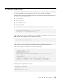
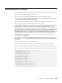
Setting parameters
In the C++ API of IBM® ILOG® CP Optimizer, you set a parameter on the optimizer with
a call to IloCP::setParameter. The first argument to this function is either IloCP::IntParam
or IloCP::NumParam. The second argument is a value of type IloInt, IloNum or the
enumerated type IloCP::ParameterValues. To set a parameter on the optimizer in the C++
API, you use the method IloCP::setParameter, for example:
IloCP cp(model);
cp.setParameter(IloCP::SearchType, IloCP::DepthFirst);
cp.solve();
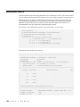
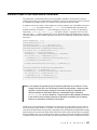
In the Java™ API of CP Optimizer, you set a parameter on the optimizer with a call to IloCP.
setParameter. The first argument to this function is either IloCP.IntParam or IloCP.
DoubleParam. The second argument is a value of type int or double or an instance of a
subclass of IloCP.ParameterValues. To set a parameter on the optimizer in the Java API,
you use the method IloCP.setParameter, for example:
IloCP cp = new IloCP();
// add variables and constraints
cp.setParameter(IloCP.IntParam.SearchType,
IloCP.ParameterValues.DepthFirst);
cp.solve();
Likewise, in the C# API of CP Optimizer, you set a parameter on the optimizer with a call
to CP.SetParameter. The first argument to this function is either CP.IntParam or CP.
DoubleParam. The second argument is a value of type Int32 or Double or an instance of a
subclass of CP.ParameterValues. To set a parameter on the optimizer in the C# API, you
use the method CP.SetParameter, for example:
CP cp = new CP();
// add variables and constraints
cp.SetParameter(CP.IntParam.SearchType,
CP.ParameterValues.DepthFirst);
cp.Solve();
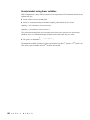
Some parameters may not be changed while there is an active search, such as between calls
to the optimizer methods startNewSearch and endSearch. You can change any limit, such
as ChoicePoinLimit, BranchLimit, TimeLimit, SolutionLimit and FailLimit during search.
The appropriate values are detailed in the IBM ILOG CP Optimizer Reference Manuals. Most
of the search parameters available for use in CP Optimizer are discussed in more detail
throughout this manual.
U S E R ' S
M A N U A L
37
Time mode parameter
IBM® ILOG® CP Optimizer uses time for both display purposes and for limiting the search.
These timings can be measured either by CPU time or by elapsed time, and the time mode
parameter defines how time is measured in CP Optimizer.
When multiple processors are available and the number of workers is greater than one, then
the CPU time can be greater than the elapsed time by a factor up to the number of workers.
In the C++ API of CP Optimizer, the time mode is controlled with the parameter
IloCP::TimeMode. A value of IloCP::CPUTime indicates that time should be measured as
CPU time, IloCP::ElapsedTime indicates that time should be measured as elapsed time.
The default is IloCP::CPUTime.
In the Java™ API of CP Optimizer, the time mode is controlled with the parameter IloCP.
IntParam.TimeMode. A value of IloCP.ParameterValues.CPUTime indicates that time should
be measured as CPU time, IloCP.ParameterValues.ElapsedTime indicates that time should
be measured as elapsed time. The default is IloCP.ParameterValues.CPUTime.
Likewise, in the C# API of CP Optimizer, the time mode is controlled with the parameter
CP.IntParam.TimeMode. A value of CP.ParameterValues.CPUTime indicates that time should
be measured as CPU time, CP.ParameterValues.ElapsedTime indicates that time should
be measured as elapsed time. The default is CP.ParameterValues.CPUTime.
38
U S E R ' S
M A N U A L
Modeling a problem with Concert
Technology
This section describes how to model a problem using Concert Technology.
In this section
Overview
Describes usage of Concert Technology classes to model a problem.
Creating the environment
Describes the use of an environment.
Managing data
Describes modeling data with arrays, sets of tuples, and piecewise linear functions.
Defining decision variables and expressions
Describes how to define decision variables and expressions in a Concert Technology model.
Declaring the objective
Describes the usage of an objective in a Concert Technology model.
Adding constraints
Describes the types of constraints available in Concert Technology for use in CP Optimizer.
Formulating a problem
Describes the method for formulating a problem.
© Copyright IBM Corp. 1987, 2009
39
Overview
In the introductory section, you learned about the three-stage method for using IBM®
ILOG® CP Optimizer. After describing your constraint satisfaction or optimization problem,
you use IBM ILOG Concert Technology classes to model the problem. A Concert Technology
model consists of a set of objects. Each decision variable, each constraint and the objective
function in a model are all represented by objects of the appropriate class. These objects
are known as modeling objects.
40
U S E R ' S
M A N U A L
Creating the environment
Describes the use of an environment.
In this section
Overview
Describes the use of an environment.
Environment and communication channels
Describes the communication channels provided in the environment.
Environment and memory management
Describes memory management as handled by the environment.
U S E R ' S
M A N U A L
41
Overview
The first step in an IBM® ILOG® Concert Technology application using the C++ API is to
create the environment, an instance of the class IloEnv.
The environment manages internal modeling issues; it handles output, memory management
for modeling objects and termination of search algorithms. In the Microsoft® .NET
Framework languages and Java™ APIs, issues regarding the environment are handled
internally.
Normally an application needs only one environment, but you can create as many
environments as you wish. Typically, the environment is created early in the main part of
an application, like this:
IloEnv env;
In the C++ API, every Concert Technology model and every optimizer object must belong
to an environment. In programming terms, when you construct a model, you must pass one
instance of IloEnv as an argument to that constructor.
In the Java API, the Concert Technology functions for creating modeling objects are defined
in the interface IloModeler and implemented in the class IloCP.
Likewise, in the C# API, the functions for creating modeling objects are defined in the
interface IModeler, and the class CP inherits them.
42
U S E R ' S
M A N U A L
Environment and communication channels
In the C++ API, an instance of IloEnv in your application initializes its default output
channels for general information, for warnings and for error messages.
Each environment maintains its own channels. The channels associated with an environment
are IloEnv::out, IloEnv::warning and IloEnv::error. By default, these output streams
are defined as std::cout. You can redirect these streams by calling IloEnv::setOut(ostream
&) and other related member functions of IloEnv.
In the Microsoft® .NET Framework languages and Java™ APIs, the native streams are used
directly. To redirect output generated by the optimizer, you use the method IloCP.setOut
in the Java API and the method CP.SetOut in the C# API. For example, in the C# API, the
output from the optimizer can be redirected to the native error stream using the following
code:
CP cp = new CP();
cp.SetOut(Console.Error);
U S E R ' S
M A N U A L
43
Environment and memory management
When your C++ application deletes an instance of IloEnv, Concert Technology will
automatically delete all models, algorithms (optimizers) and other objects depending on that
environment as well.
To allocate on the environment memory pool in C++, you must pass the environment as an
argument to the new operator:
MyObject*
myobject = new (env) MyObject();
Memory allocated in the environment is reclaimed when the environment is terminated by
the member function IloEnv::end. You must not use the delete operator for objects allocated
on the environment memory pool. The destructor of these objects will be called when the
memory is reclaimed.
To free memory used by a model in the Java™ API, you use the method IloCP.end. To free
memory used by a model in the C# API, you use the method CP.End.
Note: Environment
An instance of the class IloEnv manages the internal modeling issues, which include
handling output, memory management for modeling objects and termination of search
algorithms.
This instance is typically referred to as the environment. Normally an application needs
only one environment, but you can create as many environments as you wish.
In the C# and Java APIs, the environment object is not public. To free memory used
by a model in the Java API, you use the method IloCP.end. To free memory used
by a model in C# API, you use the method CP.End.
44
U S E R ' S
M A N U A L
Managing data
Describes modeling data with arrays, sets of tuples, and piecewise linear functions.
In this section
Overview
Describes modeling data using arrays and sets of tuples.
Arrays
Describes arrays in Concert Technology.
Sets of tuples
Describes sets of tuples in Concert Technology.
Piecewise linear functions
Describes piecewise linear functions.
Step functions
Describes step functions.
U S E R ' S
M A N U A L
45
Overview
Usually the data of a constraint programming problem must be collected before or during
the creation of the IBM® ILOG® Concert Technology representation of the model. Though,
in principle, modeling does not depend on how the data is generated and represented, this
task may be facilitated by the array and tupleset classes provided by Concert Technology.
46
U S E R ' S
M A N U A L
Arrays
The data for an IBM® ILOG® Concert Technology model is often presented in terms of
arrays.
In the Microsoft® .NET Framework languages and the Java™ APIs, the native array classes
are used to store data in arrays and are passed as arguments to many Concert Technology
functions. In the C++ API, objects of the class IloIntArray can be used to store integer
data in arrays.
Elements of the class IloIntArray can be accessed like elements of standard C++ arrays,
but the class also offers a wealth of additional functions. For example, Concert Technology
arrays are extensible; in other words, they transparently adapt to the required size when
new elements are added using the method add. Conversely, elements can be removed from
anywhere in the array with the method remove. Concert Technology arrays also provide
debugging support when compiled in debug mode by using assertion statements to ensure
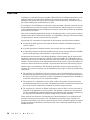
that no element beyond the array bounds is accessed. Input and output operators (that is,
operator<< and operator>>) are provided for arrays. For example, the code produces the
following output:
[1, 2, 3]
This output format can be read back in with the operator>>, for example:
std::cin >> data;
When you have finished using an array and want to reclaim its memory, call the method
end; for example, data.end. When the environment ends, all memory of arrays belonging
to that same environment is returned to the system as well. Thus, in practice you do not
need to call end on an array (or any other Concert Technology object) just before calling
IloEnv::end.
Note: Array of integer values
Arrays of integer values are represented by the class IloIntArray in the C++ API
of Concert Technology. These arrays are extensible.
When you use an array, you can access a value in that array by its index, and the
operator[] is overloaded for this purpose.
In the C# and Java APIs, the native arrays are used.
Finally, the C++ API of Concert Technology provides the template class IloArray<X> to
create array classes for your own type X. This technique can be used to generate
multidimensional arrays. All the functions mentioned here are supported for IloArray classes
except for input/output, which depends on the input and output operator being defined for
type X.
U S E R ' S
M A N U A L
47
Note: Extensible array
In the C++ API, Concert Technology provides the template class IloArray which
makes it easy for you to create classes of arrays for elements of any given class. In
other words, you can use this template to create arrays of Concert Technology objects;
you can also use this template to create arrays of arrays (that is, multidimensional
arrays).
When you use an array, you can access a value in that array by its index, and the
operator[] is overloaded for this purpose.
The classes you create in this way consist of extensible arrays. That is, you can add
elements to the array as needed.
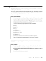
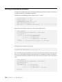
In the Java API, arrays used by a CP Optimizer method might be created as such:
int[] fixedCost ={ 1, 2, 4, 3 };
IloIntVar[] open = cp.intVarArray(4,0,1);
IloIntExpr obj = cp.prod(open, fixedCost);
In the C# API, arrays used by a CP Optimizer method might be created similarly to the
following:
int[] fixedCost ={ 1, 2, 4, 3 };
IIntVar[] open = cp.IntVarArray(4,0,1);
IIntExpr obj = cp.Prod(open, fixedCost);
48
U S E R ' S
M A N U A L
Sets of tuples
In many constraint applications, it is necessary to process a huge quantity of data. For
instance, the features of some products can be described as a relation in a database or in
text files. In this case, a useful data modeling object is a tupleset, or a set of tuples.
A tuple is an ordered set of values represented by an array. Tuples are useful for representing
allowed combinations of data in a model. A set of integer tuples in a model is represented
by an instance of a tupleset.
The elements of a tupleset are tuples of integer values, represented by arrays. The number
of values in a tuple is known as the arity of the tuple, and the arity of the tuples in a set is
called the arity of the set. (In contrast, the number of tuples in the set is known as the
cardinality of the set.)
In the C++ API of CP Optimizer, the class IloTupleSet represents tuplesets.
In the Java™ API of CP Optimizer, the interface IloTupleset represents tuplesets.
In the C# API of CP Optimizer, the interface ITupleSet represents tuplesets.
Note: Set of tuples
An integer tuple is an ordered set of values represented by an array. A set of integer
tuples in a model is represented by a tupleset.
The number of values in a tuple is known as the arity of the tuple.
Consider as an example a bicycle factory that can produce thousands of different models.
For each model of bicycle, a relation associates the features of that bicycle such as size,
weight, color and price. This information can be used in a constraint programming application
that allows a customer to find the bicycle that most closely fits a specification.
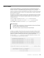
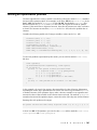
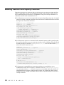
Then the tupleset bicycleSet defines the set of possible combinations of features. In the
C++ API, the tupleset is created and built as follows:
IloIntTupleSet bicycleSet(env, 5);
bicycleSet.add(IloIntArray(env, 5,
bicycleSet.add(IloIntArray(env, 5,
bicycleSet.add(IloIntArray(env, 5,
bicycleSet.add(IloIntArray(env, 5,
bicycleSet.add(IloIntArray(env, 5,
bicycleSet.add(IloIntArray(env, 5,
1,
2,
3,
4,
5,
6,
57,
57,
60,
65,
67,
70,
12,
13,
14,
14,
15,
15,
3,
5,
3,
7,
2,
2,
1490));
1340));
1790));
1550));
2070));
1990));
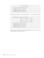
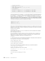
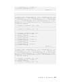
In the Java API, the tupleset is created using the method IloCP.intTable and built as follows:
IloIntTupleSet bicycleSet = cp.intTable(5);
int[][] tuples = {{1, 57, 12, 3, 1490},
{2, 57, 13, 5, 1340},
{3, 60, 14, 3, 1790},
U S E R ' S
M A N U A L
49
{4, 65, 14, 7, 1550},
{5, 67, 15, 2, 2070},
{6, 70, 15, 2, 1990}};
cp.addTuple(bicycleSet, tuples[0]);
cp.addTuple(bicycleSet, tuples[1]);
cp.addTuple(bicycleSet, tuples[2]);
cp.addTuple(bicycleSet, tuples[3]);
cp.addTuple(bicycleSet, tuples[4]);
cp.addTuple(bicycleSet, tuples[5]);
In the C# API, the tupleset is created using the method CP.IntTable and built as follows:
IIntTupleSet bicycleSet = cp.IntTable(5);
int[][] tuples = { new int [] {1, 57, 12,
new int [] {2, 57, 13,
new int [] {3, 60, 14,
new int [] {4, 65, 14,
new int [] {5, 67, 15,
new int [] {6, 70, 15,
cp.AddTuple(bicycleSet, tuples[0]);
cp.AddTuple(bicycleSet, tuples[1]);
cp.AddTuple(bicycleSet, tuples[2]);
cp.AddTuple(bicycleSet, tuples[3]);
cp.AddTuple(bicycleSet, tuples[4]);
cp.AddTuple(bicycleSet, tuples[5]);
3,
5,
3,
7,
2,
2,
1490},
1340},
1790},
1550},
2070},
1990}};
A tupleset can be used as an argument to a compatibility constraint in order to enforce the
possible combinations allowed for a solution.
50
U S E R ' S
M A N U A L
Piecewise linear functions
In IBM® ILOG® CP Optimizer, piecewise linear functions are typically used in modeling a
known function of time, for instance the cost incurred for completing an activity after a
known date. A piecewise linear function is a function defined on an interval [xmin, xmax)
which is partitioned into segments such that over each segment, the function is linear.
When two consecutive segments of the function are co-linear, these segments are merged
so that the function is always represented with the minimal number of segments.
In the C++ API of CP Optimizer, the interface IloNumToNumSegmentFunction represents
piecewise linear functions.
In the Java™ API of CP Optimizer, the class IloNumToNumSegmentFunction represents
piecewise linear functions..
In the C# API of CP Optimizer, the interface INumToNumSegmentFunction represents
piecewise linear functions.
Note: Piecewise linear function
A piecewise linear function is a function defined on an interval which is partitioned into
segments such that over each segment, the function is linear.
Each interval [x1, x2) on which the function is linear is called a segment.
When two consecutive segments of the function are co-linear, these segments are
merged so that the function is always represented with the minimal number of segments.
U S E R ' S
M A N U A L
51
Step functions
In IBM® ILOG® CP Optimizer, stepwise functions are typically used to model the efficiency
of a resource over time. A stepwise function is a special case of piecewise linear function
where all slopes are equal to 0 and the domain and image of the function are integer.
When two consecutive steps of the function have the same value, these steps are merged
so that the function is always represented with the minimal number of steps.
In the C++ API of CP Optimizer, the class IloNumToNumStepFunction represents step
functions.
In the Java™ API of CP Optimizer, the interface IloNumToNumStepFunction represents step
functions.
In the C# API of CP Optimizer, the interface INumToNumStepFunction represents step
functions.
Note: Step function
Step functions are a special case of piecewise linear function where all slopes are
equal to 0 and the domain and image of the function are integer.
Each interval [x1, x2) on which the function has the same value is called a step.
When two consecutive steps of the function have the same value, these steps are
merged so that the function is always represented with the minimal number of steps.
52
U S E R ' S
M A N U A L
Defining decision variables and expressions
Describes how to define decision variables and expressions in a Concert Technology model.
In this section
Overview
Describes using decision variables and expressions in a Concert Technology model.
Integer decision variables
Describes the usage of integer decision variables.
Interval decision variables
Describes the usage of interval decision variables.
Interval sequence decision variables
Describes the usage of interval decision sequence variables.
Expressions
Describes the usage of expressions.
Domains of variables and expressions
Describes the computation of domains of decision variables and expressions.
U S E R ' S
M A N U A L
53
Overview
Decision variables represent the unknown information in a problem. Expressions can be
built using decision variables, constants and other expressions.
54
U S E R ' S
M A N U A L
Integer decision variables
Integer decision variables represent unknown information in a problem.
Decision variables differ from normal programming variables in that they have domains of
possible values and may have constraints placed on the allowed combinations of theses
values.
These decision variables are defined by the lower bound and upper bound for the variable.
In the C++ API, the following constructor creates a constrained integer variable with bounds
-1 and 10:
IloIntVar myIntVar(env, -1, 10);
In the Java™ API, you create a constrained integer variable with bounds -1 and 10 with the
method IloCP.intVar:
IloIntVar myIntVar = cp.intVar(-1, 10);
In the C# API, you create a constrained integer variable with bounds -1 and 10 with the
method CP.IntVar:
IIntVar myIntVar = cp.IntVar(-1, 10);
In any solution, the value assigned by the optimizer to an integer decision variable must be
between the lower and upper bounds, inclusive, of that variable. During the modeling stage,
you may also modify the lower and upper bounds of a variable.
In the C++ API of CP Optimizer, the class IloIntVar represents integer decision variables.
In the Java API of CP Optimizer, the interface IloIntVar represents integer decision
variables.
In the C# API of CP Optimizer, the interface IIntVar represents integer decision variables.
Note: Integer decision variable
Integer decision variables represent unknown information in a problem.
Typically, the possible values are represented as a domain of integers with an upper
bound and a lower bound. These variables are said to be constrained because
constraints can be placed on them.
An interval variable can be specified as being optional, meaning that the interval can
be absent from the solution schedule
U S E R ' S
M A N U A L
55
Interval decision variables
An interval decision variable represents an unknown of a scheduling problem, in particular
an interval of time during which something happens (an activity is carried out) whose position
in time is unknown. An interval is characterized by a start value, an end value and a size.
The start and end of an interval variable must be in [IloIntervalMin..IloIntervalMax].
An important feature of interval decision variables is that they can be optional, that is, it is
possible to model that an interval variable can be absent from the solution schedule.
Sometimes the intensity of “work” is not the same during the whole interval. For example,
consider a worker who does not work during weekends (his work intensity during weekends
is 0%) and on Friday he works only for half a day (his intensity during Friday is 50%). For
this worker, 7 man-days work will span for longer than just 7 days. In this example 7 man-days
represent what is called the size of the interval: that is, the length of the interval would be
if the intensity function was always at 100%. To model such situations, a range for the size
of an interval variable and an integer stepwise intensity function can be specified. The length
of the interval will be at least long enough to cover the work requirements given by the
interval size, taking into account the intensity function.
In the C++ API of CP Optimizer, the class IloIntervalVar represents integer decision
variables.
In the Java™ API of CP Optimizer, the interface IloIntervalVar represents integer decision
variables.
In the C# API of CP Optimizer, the interface IIntervalVar represents integer decision
variables.
The domain of an interval variable is displayed as shown in this example:
A1[0..1: 10..990 -- (5..10)5..990 --> 25..1000]
After the name of the interval decision variable (here A1), the first range (here 0..1)
represents the domain of the boolean presence status of the interval variable. The presence
range 0..1 represents an optional interval variable whose status has still not been fixed, 0
an absent interval variable and 1 a present interval variable. An absent interval variable is
displayed as:
A1[0]
When the interval variable is possibly present, the remaining fields describe the position of
the interval variable:
♦
the first range in the remaining fields represents the domain of the interval start,
♦
the second range (between parenthesis) represents the domain of the interval size,
♦
the third range represents the domain of the interval length and
♦
the fourth and last range represents the domain of the interval end.
Note that the second range may be omitted in case the size and length of the interval variable
are necessarily equal. When the values are fixed, the ranges min..max are replaced by a
single value. For instance, the following display represents a fixed interval variable of size
5 that is present, starts at 10 and ends at 35:
56
U S E R ' S
M A N U A L
A1[1: 10 -- (5)25 --> 35]
Note: Interval decision variable
Interval decision variables represent unknowns of a scheduling problem
An interval has a start time, an end time, a size and a length. An interval variable allows
for these values to be variable in the model.
U S E R ' S
M A N U A L
57
Interval sequence decision variables
An interval sequence decision variable is defined on a set of interval variables The value of
an interval sequence variable represents a total ordering of the interval variables of the set.
Any absent interval variables are not considered in the ordering.
The sequence alone does not enforce any constraint on the relative position of interval end
points. For instance, an interval variable a could be sequenced before an interval variable
b in a sequence p without any impact on the relative position between the start/end points
of a and b (a could still be fixed to start after the end of b). Different semantics can be used
to define how a sequence constrains the positions of intervals. For instance, the no overlap
constraint on a sequence variable specifies that the interval variables in the set do not
overlap and that their start and end values are ordered according to the total ordering of
the sequence.
In the C++ API of CP Optimizer, the class IloIntervalSequenceVar represents integer
sequence decision variables.
In the Java™ API of CP Optimizer, the interface IloIntervalSequenceVar represents integer
sequence decision variables.
In the C# API of CP Optimizer, the interface IIntervalSequenceVar represents integer
sequence decision variables.
Note: Interval sequence variable
Interval sequence decision variables represent a sequences of interval variables. A
sequence can contain a subset of the variables or be empty. In a solution, the sequence
will represent a total order over all the intervals in the set that are present in the solution.
The assigned order of interval variables in the sequence does not necessarily determine
their relative positions in time in the schedule.
58
U S E R ' S
M A N U A L
Expressions
Decision variables are most often used to build expressions, which in turn are used to create
the objective and constraints of the model.
In the C++ API of IBM® ILOG® Concert Technology, expressions are generally represented
by the class IloExpr and its subclasses IloIntExpr, representing integer expressions, and
IloNumExpr, representing numeric (floating-point) expressions. Note that the parent classes
IloIntExprArg and IloNumExprArg are used internally by Concert Technology to build
expressions. You should not use IloIntExprArg or IloNumExprArg directly.
In the Java™ API of Concert Technology, expressions are generally represented by the
interfaces IloIntExpr, representing integer expressions, and IloNumExpr, representing
numeric expressions.
In the C# API of Concert Technology, expressions are generally represented by the interfaces
IIntExpr, representing integer expressions, and INumExpr, representing numeric expressions.
An integer expression can be written explicitly; for example, using the C++ API:
1*x[1] + 2*x[2] + 3*x[3]
where x is assumed to be an array of decision variables. Using the Java API, the same
expression could be written as:
cp.sum(cp.sum(cp.prod(1,x[1]),cp.prod(2,x[2])), cp.prod(3,x[3]))
Using the C# API, the same expression could be written as:
cp.Sum(cp.Sum(cp.Prod(1,x[1]),cp.Prod(2,x[2])), cp.Prod(3,x[3]))
Expressions can also be created incrementally, with a loop; for example using the C++ API:
IloIntExpr expr(env);
for (int i = 0; i < x.getSize(); ++i)
expr += data[i] * x[i];
Using the Java API, the same expression could be written as:
IloIntExpr expr = cp.constant(0);
for (int i = 0; i < x.length; ++i)
expr = cp.sum(expr, cp.prod(data[i], x[i]));
Using the C# API, the same expression could be written as:
U S E R ' S
M A N U A L
59
IIntExpr expr = cp.Constant(0);
for (int i = 0; i < x.Length; ++i)
expr = cp.Sum(expr, cp.Prod(data[i], x[i]));
In the C++ API, when you have finished using an expression (that is, you created a constraint
or objective with it) you can delete it by calling its method end, for example:
expr.end();
Many Concert Technology functions return expressions. You can build even more complicated
expressions by using the Concert Technology functions representing absolute value, integer
division, maximum, minimum and others. For example, IloAbs(x) - IloMax(y,z) is a valid
expression representing the difference between the absolute value of x and the maximum
of y and z.
Note: Expression
Values may be combined with decision variables and other expressions to form
expressions.
To combine values, variables and other expressions to form an expression, you can
use, among other functions, the operators:
♦ addition (+),
♦ subtraction (-),
♦ multiplication (*),
♦ division (/),
♦ self-assigned addition (+=) and
♦ self-assigned subtraction (-=).
Expressions are discussed in more detail in Constraints and expressions in CP Optimizer.
60
U S E R ' S
M A N U A L
Domains of variables and expressions
An integer decision variable is typically created with a lower bound and an upper bound.
The initial domain of the variable contains precisely the values from the lower bound to the
upper bound, inclusive. It is important to declare the initial domains to be as small as possible,
in order to keep the search space as small as possible. As the optimizer works to find a
solution for the problem, it will temporarily remove values from the domain of each decision
variable. The search algorithms are discussed in detail in Search in CP Optimizer.
During search, expressions have domains of possible values like decision variables. Unlike
variables, these domains are not stored but instead calculated as needed from the basic
elements of the expression.
Note: Declaring a domain
Domains for integer decision variables are declared as part of the model. In order for
the search to perform efficiently, it is important that the domains be as tight, or small,
as possible.
U S E R ' S
M A N U A L
61
Declaring the objective
An objective function is used to express the cost of each potential solution.
When an objective is added to a model, the problem is considered to be an optimization
problem. The IBM® ILOG® CP Optimizer search handles models with at most one objective
function, though the modeling API provided by Concert Technology does not impose this
restriction.
In the C++ API and the Java API, objective functions are represented by IloObjective.
In the C# API, objectives are represented by IObjective. An objective function can be
specified by creating an objective instance directly; however, it is common to use the functions
which return an instance of IloObjective. In the C++ API, the functions are IloMinimize
and IloMaximize. In the Java™ API, these functions are IloModeler.minimize and
IloModeler.maximize. In the C# API, these functions are IModeler.Minimize and IModeler.
Maximize. For example, in the C++ API, the following code defines an objective to minimize
the expression x[1] + 2*x[2] + 3*x[3]:
IloObjective obj
= IloMinimize(env,
x[1] + 2*x[2] + 3*x[3]);
Using the Java API, the same objective could be written using the method IloCP.minimize:
IloObjective obj
= cp.minimize(cp.sum(cp.sum(x[1],cp.prod(2,x[2])),cp.prod(3,x[3])));
Using the C# API, the same objective could be written using the method CP.Minimize:
IObjective obj
= cp.Minimize(cp.Sum(cp.Sum(x[1],cp.Prod(2,x[2])),cp.Prod(3,x[3])));
Note: Objective
An objective expresses the cost of possible solutions. The optimal solution to an
optimization problem is the feasible solution that, depending on the problem type,
minimizes or maximizes the cost.
After you create an objective, you must explicitly add it to the model in order for it to be
taken into account by the optimizer.
62
U S E R ' S
M A N U A L
Adding constraints
Describes the types of constraints available in Concert Technology for use in CP Optimizer.
In this section
Overview
Describes the types of constraints available in Concert Technology.
Arithmetic constraints
Describes arithmetic constraints.
Specialized constraints
Describes specialized constraints available in Concert Technology.
Combining constraints
Describes methods for combining constraints.
U S E R ' S
M A N U A L
63
Overview
IBM® ILOG® Concert Technology allows you to express constraints on decision variables
and expressions. In the C++ API and the Java™ API, constraints are represented by
IloConstraint. In the C# API, constraints are represented by the IConstraint interface.
64
U S E R ' S
M A N U A L
Arithmetic constraints
Arithmetic constraints can be created in a variety of ways.
In the C++ API, you can express constraints between expressions using the following
operators:
♦
equality (==),
♦
less than or equal to (<=),
♦
less than (<),
♦
greater than or equal to(>=),
♦
greater than (>) and
♦
not equal to (!=).
For example, you can write a constraint that one expression is not equal to another in the
C++ API:
x[1] + 2*x[2] + 3*x[3] != 4*x[1]*x[2]
Using the Java™ API, the constraint could be written as:
cp.neq(cp.sum(x[1],
cp.sum(cp.prod(2,x[2]), cp.prod(3,x[3]))) ,
cp.prod(4,cp.prod(x[1],x[2])))
Likewise, using the C# API, the constraint could be written as:
cp.Neq(cp.Sum(x[1],
cp.Sum(cp.Prod(2,x[2]), cp.Prod(3,x[3]))) ,
cp.Prod(4,cp.Prod(x[1],x[2])))
Explicitly, this constraint enforces that the values the CP Optimizer search assigns to the
decision variables x[1], x[2] and x[3] must be such that the expression x[1] + 2*x[2]
+ 3*x[3] does not equal the expression 4*x[1]*x[2].
After you create a constraint, you must explicitly add it to the model in order for it to be
taken into account by the optimizer.
For more details on expressing constraints, refer to the section Arithmetic constraints and
expressions.
U S E R ' S
M A N U A L
65
Specialized constraints
One of the most powerful features of IBM® ILOG® CP Optimizer is its provision for different
kinds of constraints.
You have already seen arithmetic constraints that enable you to combine decision variables
with the usual arithmetic operators (such as addition, subtraction, multiplication, division)
to create linear and nonlinear expressions. In addition, CP Optimizer supports constraints
on expressions that are not arithmetic: absolute value, minimum, maximum.
Specialized constraints make it possible to express complicated relations between variables,
for example, relations that would require an exponential number of arithmetic constraints
or relations that could not be expressed at all in arithmetic terms. Specialized constraints
enter into such considerations as counting values, maintaining load weights and other critical
activities.
Specialized constraints prove useful in a great many fields, in such mathematical puzzles
as magic sequences and magic squares, but also in very practical real-world problems of
allocation and scheduling. For example, the predefined “all different” constraint states that
the value assigned to each variable in an array must be different from the values assigned
to every other variable in that array.
Also, the single specialized all different constraint on n variables is logically equivalent to
(n-1)n/2 instances of the “not equal” constraint (!=), but in terms of performance, that single
constraint is much more efficient. In short, a specialized constraint such as is highly useful,
both in terms of ease of expression and computational performance.
For detailed information on the specialized constraints that are available in CP Optimizer,
refer to the section Specialized constraints on integer decision variables and Constraints
and expressions on interval decision variables in Constraints and expressions in CP Optimizer.
66
U S E R ' S
M A N U A L
Combining constraints
IBM® ILOG® CP Optimizer provides a simple yet powerful way to define a constraint by
combining other constraints.
This facility is based on the basic idea that constraints have value. The value of a constraint
is true (IloTrue in C++) if the constraint is satisfied and false (IloFalse) if the constraint
is not satisfied. Not only are they treated as if they have a Boolean value, such as true or
false, but effectively as if the value is 0 or 1.
Note: Logical constraint
A logical constraint is created by combining constraints or placing constraints on other
constraints. Logical constraints are based on the idea that constraints have value. CP
Optimizer handles constraints not only as if they have a Boolean value, such as true
or false, but effectively as if the value is 0 or 1. This allows you to combine constraints
into expressions or impose constraints on constraints.
You can use the following logical operators to combine constraints:
♦ not (!),
♦ and (&&),
♦ or (||),
♦ equivalence (==),
♦ exclusive or (!=) and
♦ implication (<=).
Furthermore, constraints can be combined using arithmetic operators.
Some of the specialized constraints cannot be used in logical constraints.
For more details on expressing logical constraints, please refer to the section Logical
constraints.
Note: Constraint
Constraints specify the restrictions on the values that may be assigned to decision
variables. To create a constraint for a model, you can:
♦ use an arithmetic operator between decision variables and expressions to return a
constraint,
♦ use a function that returns a constraint,
U S E R ' S
M A N U A L
67
♦ use a specialized constraint or
♦ use a logical operator between constraints which returns a constraint.
After you create a constraint, you must explicitly add it to the model in order for it to
be taken into account by the CP Optimizer engine.
Constraints are discussed in more detail in Constraints and expressions in CP Optimizer.
68
U S E R ' S
M A N U A L
Formulating a problem
A model is a container of modeling objects, such as objectives, variables and constraints.
You must explicitly add a constraint to the model or the IBM® ILOG® CP Optimizer search
engine will not use it in the search for a solution.
In the C++ API of CP Optimizer, a model is an instance of the class IloModel. Decision
variables, objectives and constraints can be added to the model with the method
IloModel::add.
In the Java™ API of CP Optimizer, the methods for adding object to the model are defined
in the interfaces IloModel and IloModeler and implemented in the class IloCP. In particular,
IloCP.add is one function for adding objects to the model.
Likewise, in the C# API of CP Optimizer, the methods for adding object to the model are
defined in the interface IModeler and IModelImpl and implemented in the class CP. In
particular, CP.Add is one function for adding objects to the model.
To create a model using the C++ API, the first step is to create an instance of the class
IloEnv:
IloEnv env;
(Note that creating an environment is not necessary in the C# and the Java APIs.)
The initialization of the environment creates internal data structures to be used in the rest
of the code. Once this is done, you can create model objects; here illustrated in the C++
API:
IloIntVar x(env, 0, 10);
IloConstraint ct = (x != 0);
In the Java API, you must create the IloCP object before creating the modeling objects:
IloCP cp = new IloCP();
IloIntVar x = cp.intVar(0, 10);
IloConstraint ct = cp.neq(x, 0);
Likewise in the C# API, you must create the CP object before creating the modeling objects:
CP cp = new CP();
IIntVar x = cp.IntVar(0, 10);
IConstraint ct = cp.Neq(x, 0);
Once this is done, you can create model and fill it with modeling objects; here illustrated in
the C++ API:
U S E R ' S
M A N U A L
69
IloModel model(env);
model.add(ct);
In the Java API, you have already created the IloCP object before creating the modeling
objects, so adding the constraint to the model is simply:
cp.add(ct);
Likewise in the C# API, you have already created the CP object before creating the modeling
objects, so adding the constraint to the model is simply:
cp.Add(ct);
As soon as the model is completed, you are ready to solve the problem. The processes for
searching for solutions to a model are introduced in Search in CP Optimizer.
When your problem solving is finished, you can reclaim memory for all modeling objects
and clean up internal data structures by calling IloEnv::end for every environment you
have created. This should be always be done before you exit your application.
To free memory used by a model in the Java API, you use the method IloCP.end.To free
memory used by a model in the C# API, you use the method CP.End.
Note: Model
A model is a container for modeling objects such as decision variables, objectives and
constraints.
70
U S E R ' S
M A N U A L
Constraints and expressions in CP Optimizer
This section describes the constraints and expressions available for CP Optimizer.
In this section
Overview
Describes the constraints and expressions available in CP Optimizer.
Arithmetic constraints and expressions
Describes arithmetic constraints and expressions.
Logical constraints
Describes logical constraints.
Compatibility constraints
Describes compatibility constraints.
Specialized constraints on integer decision variables
Describes specialized constraints on integer decision variables.
Constraints and expressions on interval decision variables
Describes expressions and constraints on interval decision variables.
© Copyright IBM Corp. 1987, 2009
71
Overview
This section introduces the constraints and expressions available in IBM® ILOG® CP
Optimizer. (More detail about the programming syntax of each of these features is available
in the reference manuals of CP Optimizer.) Constraints and expressions are building blocks
that can be used to create models in CP Optimizer applications.
72
U S E R ' S
M A N U A L
Arithmetic constraints and expressions
Describes arithmetic constraints and expressions.
In this section
Overview
Describes arithmetic constraints and expressions.
Arithmetic expressions
Describes arithmetic expressions.
Element expressions
Describes element expressions.
Division expression examples
Describes integer division expressions.
U S E R ' S
M A N U A L
73
Overview
An arithmetic constraint involves one or more decision variables in an arithmetic expression.
74
U S E R ' S
M A N U A L
Arithmetic expressions
2
2
An arithmetic expression consists of arithmetic terms, such as x, x , xy, or 3xy , combined
by arithmetic operations, such as addition, subtraction, multiplication and division.
Arithmetic expressions can appear in arithmetic relations, such as equality and inequality.
Arithmetic expressions may be linear (such as x < z + 3y) or nonlinear (such as
2
x < z + y*z + 3y). IBM® ILOG® CP Optimizer supports arithmetic constraints over integer
decision variables. It also supports integer or numeric (floating-point) expressions.
Note: CP Optimizer supports integer decision variables. Moreover, it is possible to constrain
floating-point expressions. It is also possible to use a floating-point expression as a
term in an objective function. For example, a floating-point cost function can be
calculated from expressions using integer decision variables, like this: cost = x/
1000 + y/3.
There are no inherent restrictions on the magnitude of arithmetic operations that you can
perform with CP Optimizer expressions and decision variables. The only limitation that you
must bear in mind in your CP Optimizer application is any possibility of overflow due to the
size and configuration of your platform (that is, limits on hardware and operating system).
For example, if you multiply the largest possible integer available on your platform by the
largest possible integer, you risk overflow because of limitations of your platform.
In the C++ API of CP Optimizer, there are overloaded operators for building arithmetic
expressions and stating constraints over them. For many arithmetic operations, such as
addition, exponentiation or modular arithmetic, there are global functions offering a variety
of signatures that accommodate many combinations of decision variables and integer or
numeric values in expressions.
In the Java™ API of CP Optimizer, there are methods to enable you to build arithmetic
expressions to state constraints. Many such methods are defined in the interface IloModeler,
implemented in the class IloCP.
Likewise, in the C# API of CP Optimizer, there are similar methods for building arithmetic
expressions and stating constraints over them. The interface IModeler defines these methods,
and the class CP inherits them.
Arithmetic operations for use in constraints summarizes the methods that support arithmetic
operations to create expressions to use in constraints. Arithmetic expressions for use in
constraints summarizes the methods and functions that return expressions for use in
constraints. Arithmetic constraints summarizes the methods that implement arithmetic
constraints. The reference manuals of the application programming interfaces (APIs)
document each method, operator or global function more fully.
In those tables, the names of applications where the expressions or constraints are used
appear in parentheses, like this (sports.cpp). The applications are part of the product,
available in the appropriate subdirectory of the examples directory of your installation.
U S E R ' S
M A N U A L
75
Arithmetic operations for use in constraints
Arithmetic operation C++ API
Java API
C# API
addition
operator+
IloModeler.sum
IModeler.Sum
IloSum
(Facility.java)
(Steelmill.cs)
operator-
IloModeler.diff
IModeler.Diff
IloDiff
(Sports.java)
(Sports.cs)
operator*
IloModeler.prod
IModeler.Prod
(Facility.java)
(Facility.cs)
(sports.cpp)
subtraction
multiplication
scalar product
IloScalProd
IloModeler.scalProd IModeler.ScalProd
(facility.cpp)
integer division
IloDiv
IloCP.div
CP.Div
(sports.cpp)
(Sports.java)
(Sports.cs)
floating-point division
operator/
IloCP.quot
CP.Quot
modular arithmetic
operator%
IloCP.modulo
CP.Modulo
(sports.cpp)
(Sports.java)
(Sports.cs)
Arithmetic expressions for use in constraints
Expression
C# API
CP.
StandardDeviation
minimum
IloMin
IloModeler.min
IModeler.Min
(talent.cpp)
(Sports.java)
(Sports.cs)
maximum
IloMax
IloModeler.max
IModeler.Max
counting
IloCount
IloCP.count
CP.Count
(teambuilding.cpp)
(Facility.java)
(Sports.cs)
IloAbs
IloModeler.abs
IModeler.Abs
(sports.cpp)
(Sports.java)
(Sports.cs)
IloElement
IloCP.element
CP.Element
element or index
U S E R ' S
Java API
standard deviation IloStandardDeviation IloCP.
standardDeviation
absolute value
76
C++ API
M A N U A L
Expression
C++ API
Java API
C# API
(Facility.java)
(Steelmill.cs)
Arithmetic constraints
Arithmetic constraint C++ API
Java API
C# API
equal to
operator== IloModeler.eq IModeler.Eq
not equal to
operator!= IloCP.neq
CP.Neq
strictly less than
operator<
IloCP.lt
CP.Lt
strictly greater than
operator>
IloCP.gt
CP.Gt
less than or equal to
operator<= IloModeler.le IModeler.Le
greater than or equal to
operator>= IloModeler.ge IModeler.Ge
U S E R ' S
M A N U A L
77
Element expressions
One arithmetic expression that deserves special consideration is the element expression.
An element expression indexes an array of values by a decision variable. In other words, it
allows you to treat the index into an array as a decision variable, as something that can be
constrained.
This kind of constrained indexing is conventionally expressed in other disciplines by a very
large number of binary (0-1) or Boolean variables. However, in IBM® ILOG® CP Optimizer
this indirect relation can be stated straight forwardly and efficiently as an expression that
can appear in constraints.
For example, in a logistics model you might use an element expression in a constraint to
index products available in warehouses. Or in a sports scheduling application, your model
might include two arrays, both listing all teams. An element expression might appear in
constraints between the two arrays to enforce which teams play each other.
In the C++ API of CP Optimizer, the global function IloElement has many signatures that
enable you to build element expressions. The index operator, operator[], allows you to
index an array of integers or constrained integer variables using a constrained integer
variable.
In the Java™ API of CP Optimizer, the methods IloCP.element allow you to build element
expressions. See the example Steelmill.java for a sample of this expression in an
application.
Likewise, in the C# API of CP Optimizer, the methods CP.Element represent element
expressions. For samples of this expression, see Teambuilding.cs, Facility.cs, or
Steelmill.cs.
78
U S E R ' S
M A N U A L
Division expression examples
Both integer division and floating-point division can be modeled in arithmetic expressions.
To clarify the distinction between integer division and floating-point division of decision
variables in constraints, consider these brief examples.
Let x be a decision variable that can assume the value 9:
♦
In the C++ API, IloIntVar x(env, 9, 9, "x");
♦
In the Java™ API, IloIntVar x = cp.intVar(9, 9);
♦
In the C# API, IIntVar x = cp.IntVar(9, 9);
Then integer division with IloDiv, or IloCP.div or CP.Div of x divided by 10 results in
the value 0 (zero).
♦
Consequently, a constraint stating "IloDiv(x, 10) == 0" is true.
♦
In contrast, a constraint stating "IloDiv(x, 10) >= 0.5" is false.
However, floating-point division with operator/, or IloCP.quot or CP.Quot of x divided
by 10 results in the value 0.9.
♦
Consequently, a constraint stating "x/10 == 0" is false.
♦
A constraint stating "x/10 >= 0.5" is true.
U S E R ' S
M A N U A L
79
Logical constraints
Logical constraints enforce logical relations.
Logical relations include:
♦
logical-and (conjunction); for example, a warehouse in a logisitics application must be in
the same region and stock the product;
♦
logical-or (disjunction); for example, a crew in a rostering application must include a
nurse or an emergency medical technician;
♦
logical-not (negation); for example, total cost must not exceed budget;
♦
if-then (implication); for example, if inventory is below threshold, then re-order.
A logical constraint makes it possible to express complicated relations between decision
variables, relations that would require an impractical number of arithmetic constraints or
relations that could not be expressed at all in arithmetic terms. Logical constraints in CP
Optimizer summarizes the logical constraints available in IBM® ILOG® CP Optimizer.
Logical constraints in CP Optimizer
Logical constraint
C++ API
Java™ API
C# API
logical-and (conjunction)
IloAnd
IloModeler.and
IModeler.And
IloOr
IloModeler.or
IModeler.Or
operator||
(Teambuilding.java) (Teambuilding.cs)
operator&&
(facility.cpp)
logical-or (disjunction)
(teambuilding.cpp)
logical-not (negation)
operator!
IloModeler.not
IModeler.Not
IloModeler.ifThen
IModeler.IfThen
IloCP.ifThenElse
(Ppp.cs)
IloNot
(talent.cpp)
logical if-then (implication) IloIfThen
(ppp.cpp)
80
U S E R ' S
M A N U A L
Compatibility constraints
IBM® ILOG® CP Optimizer offers two predefined constraints that enforce compatibility
among decision variables.
These compatibility constraints make it easier for you to declare allowed or forbidden values
that a decision variable or a group of decision variables may assume. These constraints can
apply to any number of variables simultaneously.
You use a tuple (that is, an ordered set, such as an array) to declare allowed or forbidden
values. This tuple has arity equal to the number of decision variables under consideration.
That is, the number of fields in the tuple is the same as the number of decision variables
that the constraint applies to. Each tuple declares an allowed or forbidden combination.
In the C++ API of CP Optimizer, the global functions IloAllowedAssignments and
IloForbiddenAssignments return compatibility constraints. For samples of these constraints,
see teambuilding.cpp or sports.cpp.
In the Java™ API of CP Optimizer, the methods IloCP.allowedAssignments and IloCP.
forbiddenAssignments represent compatibility constraints. For samples of these constraints,
see Teambuilding.java or Sports.java.
In the C# API of CP Optimizer, the methods CP.AllowedAssignments and CP.
ForbiddenAssignments represent compatibility constraints. For samples of these constraints,
see Teambuilding.cs or Sports.cs.
U S E R ' S
M A N U A L
81
82
U S E R ' S
M A N U A L
Specialized constraints on integer decision
variables
Describes specialized constraints on integer decision variables.
In this section
Overview
Describes the specialized constraints.
All different constraint
Describes the all-different constraint.
Minimum distance constraint
Describes the minimum distance constraint.
Packing constraint
Describes the packing constraint.
Inverse constraint
Describes the inverse constraint.
Lexicographic constraint
Describes the lexicographic constraint.
Distribution constraint
Describes the distribution constraint.
U S E R ' S
M A N U A L
83
Overview
Theoretically, these constraints can be written from elementary arithmetic constraints and
expressions, but IBM® ILOG® CP Optimizer offers you these specialized constraints, ready
to use in your application. They have been designed and implemented to reduce domains
of variables efficiently during a search.
84
U S E R ' S
M A N U A L
All different constraint
An all different constraint forces every decision variable in a given group to assume a value
different from the value of every other decision variable in that group.
In other words, no two of those decision variables will have the same integer value when
this constraint is satisfied.
For example, if the decision variables x, y and z share the domain of integers from 1 through
10, inclusive, then an all different constraint applied to x, y and z could return such solutions
as 1, 2, 3 or 4, 6, 8 or 9, 5, 2. However, 1,1, 2 would not be a solution to an all different
constraint over those three variables.
In the C++ API of CP Optimizer, the class IloAllDiff represents all different constraints.
For samples of this constraint, see teambuilding.cpp or sports.cpp.
In the Java™ API of CP Optimizer, the method IloCP.allDiff represents all different
constraints. For samples of this constraint, see Teambuilding.java or Sports.java.
In the C# API of CP Optimizer, the method CP.AllDiff represents all different constraints.
For samples of this constraint, see Teambuilding.cs or Sports.cs.
U S E R ' S
M A N U A L
85
Minimum distance constraint
A minimum distance constraint resembles an all different constraint in that it accepts a
group of decision variables (such as an array of integer decision variables) and ensures that
they differ from each other. In fact, it makes sure that they differ from one another by a
given amount, so that they are at least a certain distance apart from each other.
For example, the decision variables x, y and z share the domain of integers from 1 through
10, inclusive, and the minimum distance between them should be 3, then a minimum distance
constraint applied to x, y and z with distance 3 could return such solutions as 1, 4, 8 or
7, 10, 4. However, 2, 4, 6 would not be an acceptable solution because y would be closer to
x or z than the stipulated distance.
In the C++ API of CP Optimizer, the class IloAllMinDistance represents a minimum
distance constraint.
In the Java™ API of CP Optimizer, the method IloCP.allMinDistance represents a minimum
distance constraint.
In the C# API of CP Optimizer, the method CP.AllMinDistance represents a minimum
distance constraint.
86
U S E R ' S
M A N U A L
Packing constraint
A packing constraint maintains the load of a group of containers or bins, given a group of
weighted items and an assignment of items to containers.
To understand what a packing constraint can do, consider n items and m containers. Suppose
the containers are numbered consecutively from zero. Each item i has an integer weight wi.
Each item can go in only one container, and each item has associated with it a constrained
integer variable pi to specify in which container item i is placed. Associated with each
container j is an integer variable lj representing the load in that container. The load is the
sum of the weights of the items which have been assigned to that container. A container is
used if at least one item is placed in that container.
Given this scenario, you can use a packing constraint to do the following:
♦
You can set the capacity of each container. In other words, you can place an upper bound
on the load variable.
♦
With a packing constraint, you can also make sure that the total sum of the loads of the
containers is equal to the sum of the weights of the items being placed.
♦
You can specify the number of containers used. In fact, you can specify a particular group
of containers to use.
In the C++ API of CP Optimizer, the class IloPack returns a packing constraint. For samples
of this constraint, see ppp.cpp or steelmill.cpp.
In the Java™ API of CP Optimizer, the method IloCP.pack represents a packing constraint.
For samples of this constraint, see Ppp.java or Steelmill.java.
In the C# API of CP Optimizer, the method CP.Pack represents a packing constraint. For
samples of this constraints, see Ppp.cs or Steelmill.cs.
U S E R ' S
M A N U A L
87
Inverse constraint
An inverse constraint forces two groups of decision variables to be in strict correspondence
with each other. The two groups of decision variables are conventionally represented by
two arrays. An inverse constraint makes sure that the i-th item of one array is the inverse
of the i-th item of the other array, and vice versa.
In formal terms, if the length of the array f is n, and the length of the array invf is m, then
the inverse constraint guarantees that:
♦
for all i in the interval [0,n-1], if f[i] is in [0,m-1], then invf[f[i]]==i;
♦
for all j in the interval [0,m-1], if invf[j] is in [0,n-1], then f[invf[j]]==j.
In the C++ API of CP Optimizer, the class IloInverse represents inverse constraints. For
samples of this constraint, see sports.cpp or talent.cpp.
In the Java™ API of CP Optimizer, the method IloCP.inverse represents inverse constraints.
For a sample of this constraint, see Sports.java.
Likewise, in the C# API of CP Optimizer, the method CP.Inverse represents inverse
constraints. For a sample of this constraints, see Sports.cs.
88
U S E R ' S
M A N U A L
Lexicographic constraint
A lexicographic constraint maintains order between two groups of expressions. The two
groups of expressions are conventionally specified in two arrays that must be the same
length. A lexicographic constraint compares the expressions, index by index, to see which
is greater in lexicographic terms.
Informally, you might think of a lexicographic constraint as putting two arrays in alphabetic
order relative to each other.
In formal terms, a lexicographic constraint over two arrays x and y maintains that x is less
than or equal to y in the lexicographical sense of the term. That is, either both arrays are
equal, index by index, or there exists an index i strictly less than the length of the array x
such that for all j < i, x[j] = y[j] and x[i] < y[i].
In the C++ API of CP Optimizer, the global function IloLexicographic returns a
lexicographic constraint.
In the Java™ API of CP Optimizer, the method IloCP.lexicographic returns a lexicographic
constraint.
Likewise, in the C# API of CP Optimizer, the method CP.Lexicographic returns a
lexicographic constraint.
U S E R ' S
M A N U A L
89
Distribution constraint
A distribution constraint is a counting constraint used to count the number of occurrences
of several values among the constrained variables in an array of constrained variables. You
can also use an instance of this class to force the constrained variables of an array to assume
values in such a way that only a limited number of the constrained variables assume each
value.
To understand what a distribution constraint can do, consider an array of decision variables,
called vars. Given an array of integers values of length n called values and an array of the
same length of decision variables called cards. The i-th element of the array cards represents
the number of times the i-th element of values appears in the array of decision variables
vars.
When an instance of this class is created by a constructor with no “values” argument), then
the array of values that are being counted must be an array of consecutive integers starting
with 0 (zero). In that case, for each i, the i-th element of cards is equal to the number of
occurrences of i in the array vars.
In the C++ API of CP Optimizer, the class IloDistribute represents distribution constraints.
In the Java™ API of CP Optimizer, the method IloCP.distribute represents distribution
constraints.
Likewise, in the C# API of CP Optimizer, the method CP.Distribute represents distribution
constraints.
90
U S E R ' S
M A N U A L
Constraints and expressions on interval
decision variables
Describes expressions and constraints on interval decision variables.
In this section
Expressions on interval decision variables
Describes expressions on interval decision variables.
Forbidden values constraints
Describes forbidden value constraints on attributes of interval variables.
Precedence constraints on interval variables
Describes precedence constraints on interval variables.
Logical constraints on interval variables
Describes logical constraints on interval variables.
Constraints on groups of interval variables
Describes constraints on groups of interval variables.
Sequence constraints on interval variables and interval sequence variables
Describes sequence constraints on groups of interval variables.
Constraints and expressions on cumulative (cumul) function expressions
Describes cumulative function expressions and the expressions and constraints on cumulative
function expressions.
U S E R ' S
M A N U A L
91
Constraints on state functions
Describes constraints on state functions.
92
U S E R ' S
M A N U A L
Expressions on interval decision variables
Numerical expressions can be created from interval decision variables. These expressions
can be used to:
♦
define a term for the cost function and
♦
connect interval variables to integer and floating point expressions.
IBM® ILOG® CP Optimizer provides access to the integer expressions that represent the
start of, end of, length of and size of an interval variable. Special care must be taken in the
case of optional intervals: in this case an integer value dval must be specified which
represents the value of the expression when the interval is absent. If this value is omitted,
it is assumed to be 0.
Numerical expressions are also provided that allow you to evaluate a piecewise linear function
on these four attributes of an interval variable. A numerical value dval can be specified that
represents the value of the expression when the interval is absent. If this value is omitted,
it is assumed to be 0. The piecewise linear function used in ’eval’ expressions must be a
semi-convex function.
In the C++ API of CP Optimizer, the global functions IloStartOf, IloEndOf, IloLengthOf
and IloSizeOf return integer expressions representing the various attributes of an interval
decision variable. The global functions IloStartEval, IloEndEval, IloLengthEval and
IloSizeEval return numerical expressions representing the value of the given function
evaluated on the appropriate attribute the given of interval variable whenever the interval
variable is present.
In the Java™ API of CP Optimizer, the methods IloCP.startOf, IloCP.endOf, IloCP.
lengthOf and IloCP.sizeOf return integer expressions representing the various attributes
of an interval decision variable. The global functions IloCP.startEval, IloCP.endEval,
IloCP.lengthEval and IloCP.sizeEval return numerical expressions representing the
value of the given function evaluated on the appropriate attribute the given of interval
variable whenever the interval variable is present.
In the C# API of CP Optimizer, the methods CP.StartOf, CP.EndOf, CP.LengthOf and CP.
SizeOf return integer expressions representing the various attributes of an interval decision
variable. The global functions CP.StartEval, CP.EndEval, CP.LengthEval and CP.SizeEval
return numerical expressions representing the value of the given function evaluated on the
appropriate attribute the given of interval variable whenever the interval variable is present.
U S E R ' S
M A N U A L
93
Forbidden values constraints
It may be necessary to state that an interval cannot start, cannot end or cannot overlap a
set of fixed dates. IBM® ILOG® CP Optimizer provides constraints for modeling these
requirements. Given an interval variable and an integer stepwise function, the forbidden
start constraint states that whenever the interval is present, it cannot start at a point where
the function evaluates to zero. Given an interval variable a and an integer stepwise function
F, the forbidden end constraint states that whenever the interval is present, it cannot end
at a value t where F(t-1) = 0. Given an interval variable and an integer stepwise function,
the forbidden extent constraint states that whenever the interval is present, it cannot overlap
a point where the function evaluates to zero.
In the C++ API of CP Optimizer, the global functions IloForbidStart, IloForbidEnd and
IloForbidExtent return constraints representing restrictions on when an interval can start,
end or be placed.
In the Java™ API of CP Optimizer, the methods IloCP.forbidStart, IloCP.forbidEnd and
IloCP.forbidExtent return constraints representing restrictions on when an interval can
start, end or be placed.
In the C# API of CP Optimizer, the methods CP.ForbidStart, CP.ForbidEnd and CP.
ForbidExtent return constraints representing restrictions on when an interval can start,
end or be placed.
94
U S E R ' S
M A N U A L
Precedence constraints on interval variables
This section describes common constraints in scheduling, namely, precedence constraints.
These constraints restrict the relative temporal position of interval variables in a solution.
For instance a precedence constraint can model the fact that a given activity must end before
another given activity starts (optionally with some minimum delay). If one or both of the
interval variables of the precedence constraint is absent, then the precedence is systematically
considered to be true and thus, it does not impact the schedule.
Note: Precedence constraint
Precedence constraints are used to specify when one interval variable must start or
end with respect to the start or end time of another interval. The following types of
precedence constraints are available; if a and b denote interval variables, both interval
variables are present and delay is a number or integer expression (0 by default),
then:
♦ endBeforeEnd(a, b, delay) constrains that at least the given delay should
elapse between the end of a and the end of b. It imposes the inequality end(a)
+ delay <= end(b)
♦ endBeforeStart(a, b, delay) constrains that at least the given delay should
elapse between the end of a and the start of b. It imposes the inequality end(a)
+ delay <= start(b).
♦ endAtEnd(a, b, delay) constrains the given delay to separate the end of a
and the end of b. It imposes the equality end(a) + delay == end(b).
♦ endAtStart(a, b, delay) constrains the given delay to separate the end of
a and the start of b. It imposes the equality end(a) + delay == start(b).
♦ startBeforeEnd(a, b, delay) constrains that at least the given delay should
elapse between the start of a and the end of b. It imposes the inequality start(a)
+ delay <= end(b).
♦ startBeforeStart(a, b, delay) constrains that at least the given delay
should elapse between the start of a and the start of b. It imposes the inequality
start(a) + delay <= start(b).
♦ startAtEnd(a, b, delay) constrains the given delay to separate the start of
a and the end of b. It imposes the equality start(a) + delay == end(b).
♦ startAtStart(a, b, delay) constrains the given delay to separate the start
of a and the start of b. It imposes the equality start(a) + delay == start
(b).
If either interval a or b is not present in the solution, the constraint is automatically
satisfied, and it is as if the constraint was never imposed.
U S E R ' S
M A N U A L
95
In the C++ API of CP Optimizer, the global functions IloEndBeforeEnd, IloEndBeforeStart,
IloEndAtEnd, IloEndAtStart, IloStartBeforeEnd, IloStartBeforeStart, IloStartAtEnd
and IloStartAtStart return precedence constraints.
In the Java™ API of CP Optimizer, the methods IloCP.endBeforeEnd, IloCP.
endBeforeStart, IloCP.endAtEnd, IloCP.endAtStart, IloCP.startBeforeEnd, IloCP.
startBeforeStart, IloCP.startAtEnd and IloCP.startAtStart return precedence
constraints.
In the C# API of CP Optimizer, the methods CP.EndBeforeEnd, CP.EndBeforeStart, CP.
EndAtEnd, CP.EndAtStart, IloCP.startBeforeEnd, IloCP.startBeforeStart, IloCP.
startAtEnd and IloCP.startAtStart return precedence constraints.
96
U S E R ' S
M A N U A L
Logical constraints on interval variables
The presence status of interval variables can be restricted by logical constraints. The presence
constraint states that a given interval variable must be present. Of course, this constraint
may be used in logical constraints. For example, given two optional intervals a and b, a
logical constraint could be that if interval a is present then b must be present too. This can
be modeled using the presence constraint.
In the C++ API of CP Optimizer, the global function IloPresenceOf returns a constraint
that states that a given interval must be present.
In the Java™ API of CP Optimizer, the method IloCP.presenceOf returns a constraint that
states that a given interval must be present.
In the C# API of CP Optimizer, the method CP.PresenceOf returns a constraint that states
that a given interval must be present.
U S E R ' S
M A N U A L
97
Constraints on groups of interval variables
Constraints over groups of intervals allow hierarchical creation of the model by
“encapsulating” a group of interval variables by one “high level” interval.
The spanning constraint states that a given interval spans over all present intervals from a
given set. That is, the given interval starts together with the first present interval from the
set and ends together with the last one.
In the C++ API of CP Optimizer, the class IloSpan represents a spanning constraint.
In the Java™ API of CP Optimizer, the method IloCP.span returns a spanning constraint.
In the C# API of CP Optimizer, the method CP.Span returns a spanning constraint.
The alternative constraint models an exclusive alternative among a set of intervals. If a given
interval a is present then exactly one of the intervals of the set is present and interval a
starts and ends together with this chosen one.
In the C++ API of CP Optimizer, the class IloAlternative represents an alternative
constraint.
In the Java API of CP Optimizer, the method IloCP.alternative returns an alternative
constraint.
In the C# API of CP Optimizer, the method CP.Alternative returns an alternative constraint.
The synchronization constraint makes the intervals in the given set start and end together
with an interval a, if a is present.
In the C++ API of CP Optimizer, the class IloSynchronize represents a synchronization
constraint.
In the Java API of CP Optimizer, the method IloCP.synchronize returns a synchronization
constraint.
In the C# API of CP Optimizer, the method CP.Synchronize returns a synchronization
constraint.
98
U S E R ' S
M A N U A L
Sequence constraints on interval variables and interval sequence
variables
An interval sequence variable alone does not enforce any constraint on the relative position
of the end points of the interval variables. For instance, an interval variable a could be
sequenced before an interval variable b in a sequence p without any impact on the relative
position between the start/end points of a and b (a could still be fixed to start after the end
of b). Different semantics can be used to define how a sequence constrains the positions of
intervals.
There are four sequencing constraints available on sequence variables. The first in sequence
constraint on an interval variable and an interval sequence variable states that if the interval
variable is present, then it will be the first interval of the sequence. The last in sequence
constraint on an interval variable and an interval sequence variable states that if an interval
variable is present, it will be the last interval of the sequence. The before constraint on an
interval sequence variable and two interval variable states that if both interval variables are
present, then the first interval variable will appear in the sequence before the other interval.
The previous constraint on an interval sequence variable and two interval variable states
that if both interval variables are present then the first interval variable will be just before
the other in the sequence, that is, it will appear before the second and no other interval will
be sequenced between the two intervals.
In the C++ API of CP Optimizer, the functions IloFirst, IloLast, IloBefore and IloPrev
represent the sequencing constraints.
In the Java™ API of CP Optimizer, the methods IloCP.first, IloCP.last, IloCP.before
and IloCP.prev represent the sequencing constraints.
In the C# API of CP Optimizer, the methods CP.First, CP.Last, CP.Before and CP.Prev
represent the sequencing constraints.
The no overlap constraint on an interval sequence variable p states that the sequence defines
a chain of non-overlapping intervals, any interval in the chain being constrained to end
before the start of the next interval in the chain. This constraint is typically useful for
modeling disjunctive resources.
A transition distance matrix can be specified, which defines the minimal distance that must
separate two consecutive intervals in the sequence.
In the C++ API of CP Optimizer, the class IloNoOverlap represents a no overlap constraint.
In the Java API of CP Optimizer, the method IloCP.noOverlap returns a no overlap
constraint.
In the C# API of CP Optimizer, the method CP.NoOverlap returns a no overlap constraint.
U S E R ' S
M A N U A L
99
100
U S E R ' S
M A N U A L
Constraints and expressions on cumulative
(cumul) function expressions
Describes cumulative function expressions and the expressions and constraints on cumulative
function expressions.
In this section
Overvew
Gives an overview of cumulative function expressions and the expressions and constraints
on cumulative function expressions.
Cumul function expressions
Describes cumul functions and elementary cumul functions.
Elementary cumul function expressions
Describes the elementary cumul functions.
Expressions on cumul function expressions
Describes expressions on cumul functions.
Constraints on cumul function expressions
Describes constraints on cumul functions.
U S E R ' S
M A N U A L
101
Overvew
This section describes cumulative function expressions and the expressions and constraints
on cumulative function expressions. In the rest of this manual, the term “expression” is often
dropped from “cumul function expression” to increase readability.
102
U S E R ' S
M A N U A L
Cumul function expressions
In scheduling problems involving cumulative resources (also known as renewable resources),
the cumulated usage of the resource by the activities is usually represented by a function
of time. An activity usually increases the cumulated resource usage function at its start time
and decreases it when it releases the resource at its end time (pulse function). For resources
that can be produced and consumed by activities (for instance the content of an inventory
or a tank), the resource level can also be described as a function of time, production activities
will increase the resource level whereas consuming activities will decrease it. In these type
of problems, the cumulated contribution of activities on the resource can be represented by
a function of time and constraints can be posted on this function, for instance a maximal or
a safety level.
IBM® ILOG® CP Optimizer introduces the notion of cumulative (cumul) function expression
which is a function that represents the sum of individual contributions of intervals. A family
of elementary cumul function expressions describes the individual contribution of an interval
variable (or a fixed interval of time). These expressions cover the main use-cases mentioned
above: pulse for usage of a cumulative resource, step for resource production/consumption.
When the elementary cumul functions that define a cumul function are fixed (and thus, so
are their related intervals), the expression is fixed. CP Optimizer provides several constraints
over cumul functions. These constraints allow restriction of the possible values of the function
over the complete horizon or over some fixed or variable interval. For applications where
the actual quantity of resource that is used, produced or consumed by intervals is an unknown
of the problem, expressions are available for constraining these quantities.
In the C++ API of CP Optimizer, the class IloCumulFunctionExpr represents a cumul
function expression.
In the Java™ API of CP Optimizer, the method IloCP.cumulFunctionExpr returns a cumul
function expression.
In the C# API of CP Optimizer, the method CP.CumulFunctionExpr returns a cumul function
expression.
U S E R ' S
M A N U A L
103
Elementary cumul function expressions
The effects of an interval variable on a cumul function are modeled using elementary cumul
functions. An elementary pulse function increases or decreases the level of the function by
a given amount for the length of a given interval variable or fixed interval. An elementary
step function increases or decreases the level of the function by a given amount at a given
time. An elementary step at start function increases or decreases the level of the function
by a given amount at the start of a given interval variable. An elementary step at end function
increases or decreases the level of the function by a given amount at the end of a given
interval variable.
In the C++ API of CP Optimizer, the functions IloPulse, IloStep, IloStepAtStart and
IloStepAtEnd return elementary cumul functions.
In the Java™ API of CP Optimizer, the methods IloCP.pulse, IloCP.step, IloCP.
stepAtStart and IloCP.stepAtEnd return elementary cumul functions.
In the C# API of CP Optimizer, the methods CP.Pulse, CP.Step, CP.StepAtStart and CP.
StepAtEnd return elementary cumul functions.
104
U S E R ' S
M A N U A L
Expressions on cumul function expressions
The actual height of a cumul function may be an unknown of the problem. CP Optimizer
provides a family of integer expressions to control this height. Some of these expressions
define a range of possible values for the actual height of the function when a given interval
variable is present. The actual height is an unknown of the problem, and some integer
expressions to control this height are provided.
The height at start expression returns the value of the contribution of the given interval a
to the given cumul function evaluated at the start of a that is, it measures the contribution
of interval a to the cumul function at its start point. Similarly, the height at end expression
returns the value of the contribution of the given interval a to the given cumul function
evaluated at the end of a. An additional integer value dval can be specified at the construction
of the expression in which case that will be the value returned by the expression when the
interval is absent otherwise, if no value is specified, the expression will be equal to 0 when
the interval is absent.
In the C++ API of CP Optimizer, the functions IloHeightAtStart and IloHeightAtEnd
return integer expressions representing the total contribution of the start or and of an
interval variable to a cumul function.
In the Java™ API of CP Optimizer, the methods IloCP.heightAtStart and IloCP.
heightAtEnd return integer expressions representing the total contribution of the start or
and of an interval variable to a cumul function.
In the C# API of CP Optimizer, the methods CP.HeightAtStart and CP.HeightAtEnd return
integer expressions representing the total contribution of the start or and of an interval
variable to a cumul function.
U S E R ' S
M A N U A L
105
Constraints on cumul function expressions
Cumul functions can be constrained to evaluate within a certain range of values for a fixed
interval or an interval variable. A simple less than or equal constraint on inequality constraint
on a cumul function states that the domain of values of the cumul function cannot exceed
the given value anywhere along the temporal axis. An “always equal” range constraint on
a cumul function states that the cumul expression function must evaluate to a given value
everywhere on a fixed interval or from the start to end of a given interval variable. An “always
in” range constraint on a cumul function states that the domain of the cumul expression
function must evaluate to within a certain range at each point within a fixed interval or from
the start to end of a given interval variable.
Range constraints on cumul functions cannot be used in logical constraints of CP Optimizer,
because any logical constraint involving interval variables must be captured via the presence
Boolean value on the interval handled by the presence constraint.
In the C++ API of CP Optimizer, the functions IloAlwaysIn, IloAlwaysEqual, operator<=
and operator>= return range constraints on cumul functions.
In the Java™ API of CP Optimizer, the methods IloCP.alwaysIn, IloCP.alwaysEqual,
IloCP.le and IloCP.ge return range constraints on cumul functions.
In the C# API of CP Optimizer, the methods CP.AlwaysIn, CP.AlwaysEqual, CP.Le and CP.
Ge return range constraints on cumul functions.
106
U S E R ' S
M A N U A L
Constraints on state functions
A state function is a decision variable whose value is a set of non-overlapping intervals over
which the function maintains a particular non-negative integer state. In between those
intervals, the state of the function is not defined, typically because of an ongoing transition
between two states.
A set of constraints is available to restrict the evolution of a state function. These constraints
allow you to specify that:
♦
the state of the function must be defined and should remain equal to a given state
everywhere over a given fixed or variable interval.
♦
the state of the function must be defined and should remain constant (no matter its value)
everywhere over a given fixed or variable interval.
♦
the state of the function must be defined and should remain constant (no matter its value)
everywhere over a given fixed or variable interval.
♦
intervals requiring the state of the function to be defined cannot overlap a given fixed or
variable interval.
♦
everywhere over a given fixed or variable interval, the state of the function, if defined,
must remain within a given range of states.
In the C++ API of CP Optimizer, the functions IloAlwaysIn, IloAlwaysEqual,
IloAlwaysConstant and IloAlwaysNoState return state constraints.
In the Java™ API of CP Optimizer, the methods IloCP.alwaysIn, IloCP.alwaysEqual,
IloCP.alwaysConstant and IloCP.alwaysNoState return state constraints.
In the C# API of CP Optimizer, the methods CP.AlwaysIn, CP.AlwaysEqual, CP.
AlwaysConstant and CP.AlwaysNoState return state constraints.
U S E R ' S
M A N U A L
107
108
U S E R ' S
M A N U A L
Constraint propagation in CP Optimizer
This section describes constraint propagation in CP Optimizer.
In this section
Overview
Describes constraint propagation in CP Optimizer.
Basics of constraint propagation
Describes the basics of constraint propagation.
Domain reduction
Describes the principles of domain reduction.
Constraint propagation
Describes the general constraint propagation algorithm.
Propagation of arithmetic constraints
Describes propagation of arithmetic constraints.
Propagation of logical constraints
Describes propagation of logical constraints.
Propagation of specialized constraints and expressions
Describes the propagation of specialized constraints and expressions.
Constraint aggregation
Describes constraint aggregation.
© Copyright IBM Corp. 1987, 2009
109
Overview
IBM® ILOG® CP Optimizer solves a model using constraint propagation and constructive
search with search strategies. This section describes constraint propagation in detail and
illustrates the domain reduction process for most of the constraints that are available in CP
Optimizer. The algorithms that are available for searching for solutions will be described in
the following sections.
The examples in this section are for illustrating the effect of different propagation levels
and have been written using the C++ API.
110
U S E R ' S
M A N U A L
Basics of constraint propagation
The term constraint propagation refers to two distinct processes, domain reduction and
communicating these reductions amongst the constraints. These two processes are described
in a general sense first, then the details of domain reduction for each type of constraint
follow.
U S E R ' S
M A N U A L
111
Domain reduction
Each decision variable in an IBM® ILOG® Concert Technology model has a domain that is
the set of its possible values.
For instance, the domain of the decision variable
IloIntVar x(env, -1, 2);
is the set of values {-1, 0, 1, 2} , represented as [-1..2].
Note: In IBM ILOG CP Optimizer and Concert Technology, square brackets denote the
domain of decision variables. For example, [5 12] denotes a domain as a set consisting
of precisely two integers, 5 and 12. In contrast, [5..12] denotes a domain as a range
of integers, that is, the interval of integers from 5 to 12, so it consists of 5, 6, 7, 8, 9,
10, 11 and 12.
A constraint is stated over one or more decision variables and restricts the possible
assignments of values to these variables. The possible assignments are the solutions of the
constraint. For instance, the constraint x <= y allows the assignments x = 0, y = 1 or x =
2, y = 2 but not x = 3, y = 2.
A constraint can perform domain reduction on its decision variables to eliminate from their
domains values that do not belong to a solution of the constraint. When the domain reduction
algorithm is such that it removes all the values that do not belong to a solution, the process
is called full domain reduction. Full domain reduction sometimes can be very costly in terms
of computation time, so, in practice, the domain reduction performed by a constraint does
not necessarily eliminate all inconsistent values.
As an example, consider the variables x and y, each of which has the initial domain [1..10]
and the constraint x + y <= 5.
The domain of each variable is the set of integer values from 1 to 10. A solution to the
constraint x + y <= 5 is the assignment to x and y any combination of values from the set
{1, 2, 3, 4}. The assignment x = 5 does not lead to a solution for this constraint as there is
no value in the domain of y that satisfies the constraint when x = 5. A full domain reduction
for this constraint eliminates all values greater than 4 from the domains of x and y, and thus
the domains of x and y are reduced to the interval [1..4].
112
U S E R ' S
M A N U A L
Constraint propagation
Constraint propagation is the process of communicating the domain reduction of a decision
variable to all of the constraints that are stated over this variable.
This process can result in more domain reductions. These domain reductions, in turn, are
communicated to the appropriate constraints. This process continues until no more variable
domains can be reduced or when a domain becomes empty and a failure occurs. An empty
domain during the initial constraint propagation means that the model has no solution.
For example, consider the decision variables y with an initial domain [0..10], z with an initial
domain [0..10] and t with an initial domain [0..1], and the constraints
y + 5*z <= 4
t != z
t != y
over these three variables.
The domain reduction of the constraint y + 5*z <= 4 reduces the domain of y to [0..4] and
z to [0]. The variable z is thus fixed to a single value. Constraint propagation invokes domain
reduction of every constraint involving z. Domain reduction is invoked again for the constraint
y + 5*z <= 4, but the variable domains cannot be reduced further. Domain reduction of the
constraint t != z is invoked again, and because z is fixed to 0, the constraint removes the
value 0 from the domain of t. The variable t is now fixed to the value 1, and constraint
propagation invokes domain reduction of every constraint involving t, namely t != z and t
!= y. The constraint that can reduce domains further is t != y. Domain reduction removes
the value 1 from the domain of y.
Constraint propagation is performed on constraints involving y; however, no more domain
reduction can be achieved and the final domains are:
♦
y = [0 2..4],
♦
z = [0] and
♦
t = [1].
To invoke the constraint propagation process in IBM® ILOG® CP Optimizer, the propagate
function of the optimizer object is called. In the C++ API, this function is IloCP::propagate;
in the Java™ API, this function is IloCP.propagate; and in the C# API, this function is CP.
Propagate. This function invokes domain reduction on every constraint of the model and
propagates the domain reductions. It returns true (IloTrue in the C++ API) if propagation
succeeds; in other words, if no empty domains result. It returns false (IloFalse in the C++
API) otherwise.
As an example using the C++ API, a code that invokes propagation on the model above is;
IloIntVar y(env, 0, 10);
IloIntVar z(env, 0, 10);
IloIntVar t(env, 0, 1);
IloModel model(env);
U S E R ' S
M A N U A L
113
model.add(y + 5*z <= 4);
model.add(t != z);
model.add(t != y);
IloCP cp(model);
if (cp.propagate()){
cp.out() << “ Propagation
cp.out() << “ Domain of y
cp.out() << “ Domain of z
cp.out() << “ Domain of t
}else{
cp.out() << “ Propagation
}
succeeded: “ << std::endl;
= “ << cp.domain(y) << std::endl;
= “ << cp.domain(z) << std::endl;
= “ << cp.domain(t) << std::endl;
failed” << std::endl;
The call to the method IloCP::domain(IloIntVar x) is directed to an output stream to
display the current domain of the decision variable x. Running this code produces the output:
Propagation
Domain of y
Domain of z
Domain of t
114
U S E R ' S
succeeded:
= [0 2..4]
= [0]
= [1]
M A N U A L
Propagation of arithmetic constraints
In the C++ API, IBM® ILOG® CP Optimizer can handle arithmetic expressions created
with the operators +, -, * and /. Arithmetic constraints are created with arithmetic
expressions and operators like ==, <=, >=, < and >.
For example, the constraint 17*p*q + x/y <= 100, where p, q, x and y are decision variables,
can be handled by CP Optimizer. These operators are discussed in more detail in the section
Arithmetic constraints and expressions. The Java API and C# API equivalents of the operators
are listed there as well.
Apart from a few cases that are described below, arithmetic constraints do not achieve full
domain reduction because there does not always exist an efficient algorithm for full domain
reduction. Thus, domain reduction is mostly applied to bounds of decision variables and is
called bound reduction. Bound reduction is considered as a good trade-off between the
number of values removed and the efficiency of the domain reduction algorithm.
For example, consider the model:
IloIntVar x(env, -7, 7);
IloIntVar y(env, -7, 7);
IloModel model(env);
model.add(0.5*x + 3*y == 5);
The two solutions of this model are x = -2, y = 2 and x = 4, y = 1. Full constraint propagation
would give the domain of x as [-2 4] and the domain of y as [1 2]. However, ILOG CP Optimizer
does not perform this domain reduction. The constraint propagation engine does not create
“holes” in the domain of x. The reduced domain of x is [-2..4].
There are exceptions to this behavior. These are binary constraints of the form y == a*x +
b, where y and x are variables and a and b are numerical values. In this case, full domain
reduction is achieved.
For instance consider the constraint y == 2*x over the variables x with domain [1..3] and y
with domain [0..10]. This constraint forces y to be even. Full domain reduction is performed
and reduces the domain of y to [2 4 6]. The main reason for achieving full domain reduction
in this case is that it does not hurt the efficiency of constraint propagation, and it can be
effective to propagate holes in domains from a constraint to another when there are linking
constraints like x == y in a model.
Another case is that of linear inequalities such as x + 3y - 4z <= 10. Achieving bound
reduction for these constraints is sufficient to achieve full domain reduction.
CP Optimizer provides bound reduction for expressions such as absolute value, minimum,
maximum and piecewise linear functions. On these expressions, achieving bound reduction
is sufficient to maintain full domain reduction.
In the C++ API, an absolute value expression is created with the function IloAbs. Consider
the following code:
IloIntVar x(env, -10, 20);
IloIntVar y(env, -3, 4);
IloModel model(env);
U S E R ' S
M A N U A L
115
model.add(y == IloAbs(x));
IloCP cp(model);
cp.propagate();
cp.out() << “ Domain of x = “ << cp.domain(x) << std::endl;
cp.out() << “ Domain of y = “ << cp.domain(y) << std::endl;
Running this code, the domains of both x and y are reduced. The domain of y is reduced so
that it is positive and the domain of x is reduced to take into account the maximum value of
y:
Domain of x = [-4..4]
Domain of y = [0..4]
In the C++ API, minimum and maximum values expressions over a set of variables are
created with the IloMin and IloMax expressions. For example consider the model:
IloIntVar x(env, 0, 10);
IloIntVar y(env, 4, 6);
IloIntVar u(env, 2, 10);
IloModel model(env);
model.add(u == IloMin(x, y));
IloCP cp(model);
cp.propagate();
cp.out() << “ Domain of x = “ << cp.domain(x) << std::endl;
cp.out() << “ Domain of y = “ << cp.domain(y) << std::endl;
cp.out() << “ Domain of u = “ << cp.domain(u) << std::endl;
The value of u cannot exceed the smallest upper bound of x and y, that is 6. Moreover, x nor
y cannot have a value smaller than the lower bound of u, which is 2. The domains of the
variables after running this code are:
Domain of x = [2..10]
Domain of y = [4..6]
Domain of u = [2..6]
116
U S E R ' S
M A N U A L
Propagation of logical constraints
IBM® ILOG® CP Optimizer can process logical constraints. Logical constraints are stated
over arithmetic constraints and also over some specialized constraints.
The connectors for creating logical constraints are described in detail in Logical constraints.
♦
negation (!),
♦
conjunction (&&),
♦
disjunction (||),
♦
implication (<=),
♦
equivalence (==) and
♦
exclusive or (!=).
The semantics of these connectors are the usual logical semantics. The arguments of these
connectors are constraints that, in turn, possibly could be logical constraints. For instance,
consider two tasks whose durations are represented by the integer values dx and dy and
whose starting dates are represented by the decision variables x and y. To model the
constraint that the two tasks do not overlap, you can state the disjunction:
(x >= y + dy) || (y >= x + dx)
To impose this constraint only when another condition is true (for example when z == 3),
you can write the logical constraint (shown here using the C++ API):
IloIfThen(env, z == 3, (x >= y + dy) || (y >= x + dx))
To understand the domain reduction achieved by these constraints, it is important to observe
that a constraint has a truth value. Depending on the domains of the variables, the truth
value of a constraint is true when the constraint is definitely satisfied. The truth value is
false when the constraint is definitely violated. Otherwise, both values are possible.
Consider, for instance, the constraint z == 3. It has a truth value of false when the domain
of z is [0..2], that is, when it does not contain 3. It has a truth value of true when z is fixed
to 3. The truth value of this constraint is not yet determined when the domain of z contains
the value 3 and at least one other value. The truth value is undetermined if the domain of z
is [2..3]; it is not yet known if the constraint z == 3 will be satisfied (z = 3) or violated (z =
2).
In practice, each constraint appearing in a logical expression is associated with a boolean
decision variable whose value is the truth value of the constraint. These boolean variables
are mentioned in the search log as additional variables.
Here is an example of a logical model using the C++ API:
IloIntVar x(env, 0, 5);
IloIntVar y(env, 7, 20);
IloIntVar z(env, -10, 20);
U S E R ' S
M A N U A L
117
IloModel model(env);
model.add(x >= y || z < 7);
model.add(IloIfThen(env, z !=
IloCP cp(model);
cp.propagate();
cp.out() << “ Domain of x = “
cp.out() << “ Domain of y = “
cp.out() << “ Domain of z = “
10, y == 10));
<< cp.domain(x) << std::endl;
<< cp.domain(y) << std::endl;
<< cp.domain(z) << std::endl;
In the first disjunction, the constraint x >= y is obviously violated. To satisfy this disjunction,
the constraint z < 7 is imposed. This forces the maximum of the domain of z to be 6. The
domain reduction of the implication (IloIfThen) constraint is invoked since the domain of
z has changed. The left member of the implication (z != 10) is now satisfied and the constraint
imposes the constraint y == 10 which reduces the domain of y. No more domain reduction
can be done at this point and this code produces the output:
Domain of x = [0..5]
Domain of y = [10]
Domain of z = [-10..6]
This manner of reducing domains by imposing constraints is very efficient, but it has some
limitations. It reacts only to violation or satisfaction of constraints. For instance, the domain
reduction of the constraint
(x == 2) || (x == 3)
will not reduce the domain of x to [2..3]. It waits for one of the constraints to be violated
before imposing the other one.
Since any arithmetic or logical constraint can have a truth value, these constraints can
appear where any other expression can appear. In particular, such a constraint can be
combined in an arithmetic expression. An expression such as
1 + (x < 7)
is a valid expression and can be handled by CP Optimizer. Constraints can be created over
these expressions. For instance, recall the disjunction
(x >= y + dy) || (y >= x + dx)
It can be expressed by the constraint
(x >= y + dy) + (y >= x + dx) >= 1
Since only one of the disjunction members can be true, it can also be stated as
(x >= y + dy) + (y >= x + dx) == 1
Similarly, the implication (here in the C++ API)
IloIfThen(env, z == 3, (x >= y + dy) || (y >= x + dx))
can be expressed by
(z == 3) <= ((x >= y + dy) || (y >= x + dx))
or by
118
U S E R ' S
M A N U A L
(z == 3) <= (x >= y + dy) + (y >= x + dx)
A typical application of such constraints are cardinality constraints. When among a set of
constraints at least two of them must be true, one can state a constraint like
(x >= y[0]) + (x >= y[1]) + (x >= y[2]) + (x >= y[3]) + (x >= y[4]) >= 2
The statement of this constraint with only logical connectors is possible but would need a
large number of disjunctions.
U S E R ' S
M A N U A L
119
120
U S E R ' S
M A N U A L
Propagation of specialized constraints and
expressions
Describes the propagation of specialized constraints and expressions.
In this section
Overview
Describes the propagation of specialized constraints and expressions.
Inference levels
Describes constraint propagation inference levels.
The element expression
Describes the effect of various inference levels on the propagation of the element expression.
The counting expression
Describes the effect of various inference levels on the propagation of the counting expression.
The distribution constraint
Describes the effect of various inference levels on the propagation of the distribution
constraint.
The compatibility and incompatibility constraints
Describes the effect of various inference levels on the propagation of the compatibility and
incompatibility constraints.
U S E R ' S
M A N U A L
121
Overview
A fundamental and powerful feature of IBM® ILOG® CP Optimizer are the predefined
specialized constraints. In theory, basic constraints like arithmetic and logical ones can
model any kind of constraint. A specialized constraint is equivalent to a set of arithmetic or
logical constraints. In most of the cases, the specialized constraint achieves more domain
reduction than the equivalent set of basic constraints and performs domain reduction more
efficiently.
Specialized constraints prove useful in the practical real-world problems of allocation and
scheduling. These constraints make it possible to express complicated relations between
decision variables, for example, relations that would require a huge number of arithmetic
constraints. Specialized constraints enter into such considerations as counting values,
maintaining load weights and other such critical activities.
A typical example of the gain specialized constraints can provide is illustrated with the
following model implemented using the C++ API:
IloIntVar x(env, 1, 2);
IloIntVar y(env, 1, 2);
IloIntVar z(env, 1, 2);
IloModel model(env);
model.add(x != y);
model.add(x != z);
model.add(y != z);
Each decision variable has the values 1 and 2 in its domain, and the constraints state that
the variables must be all assigned different values. This model clearly has no solution.
However, no constraint can perform domain reduction. Examining the constraint x != y,
both x = 1, y = 2 and x = 2, y = 1 are solutions. Therefore, no value can be removed from
domains of x or y if the constraints are considered independently.
To achieve more domain reduction by having a more global view on this model, the three
constraints need to be replaced by the all different constraint:
model.add(IloAllDiff(env, IloIntVarArray(env, 3, x, y, z)));
In order to achieve full domain reduction, the inference level of this constraint, that is the
strength of its domain reduction, must be set to the extended level by changing the parameter
IloCP::AllDiffInferenceLevel:
cp.setParameter(IloCP::AllDiffInferenceLevel, IloCP::Extended);
Invoking propagation by running the code:
IloCP cp(model);
cp.setParameter(IloCP::AllDiffInferenceLevel, IloCP::Extended);
122
U S E R ' S
M A N U A L
if (cp.propagate()){
cp.out() << “ Propagation
cp.out() << “ Domain of x
cp.out() << “ Domain of y
cp.out() << “ Domain of z
}else{
cp.out() << “ Propagation
}
succeeded: “ << std::endl;
is “ << cp.domain(x) << std::endl;
is “ << cp.domain(y) << std::endl;
is “ << cp.domain(z) << std::endl;
failed” << std::endl;
produces the output:
Propagation failed
because the domain reduction has now created an empty domain for one the variables x, y,
or z.
U S E R ' S
M A N U A L
123
Inference levels
The inference level of a constraint, that is, the strength of the domain reduction is achieves,
is controlled by tuning parameters. There is a parameter for each specialized constraint
whose inference level can be changed.
In the C++ API, these parameters are:
♦
IloCP::AllDiffInferenceLevel,
♦
IloCP::DistributeInferenceLevel,
♦
IloCP::CountInferenceLevel,
♦
IloCP::SequenceInferenceLevel,
♦
IloCP::AllMinDistanceInferenceLevel,
♦
IloCP::ElementInferenceLevel,
♦
IloCP::PrecedenceInferenceLevel,
♦
IloCP::IntervalSequenceInferenceLevel,
♦
IloCP::NoOverlapInferenceLevel,
♦
IloCP::CumulFunctionInferenceLevel and
♦
IloCP::StateFunctionInferenceLevel.
For the Java™ API, the inference level parameter for the all different constraint is IloCP.
IntParam.AllDiffInferenceLevel. For the C# API, the inference level for the all different
constraint is CP.IntParam.AllDiffInferenceLevel. The parameters in the C# API and
the Java API for the other specialized constraints are similarly formed.
The effects of changing the values of these inference level parameters will be described in
the following sections.
In the C++ API, the possible values of these parameters are:
♦
IloCP::Default,
♦
IloCP::Low,
♦
IloCP::Basic,
♦
IloCP::Medium and
♦
IloCP::Extended.
For the Java API, the default value is IloCP.ParameterValues.Default. For the C# API,
the default inference level is CP.ParameterValues.Default.
The strength of the domain reduction increases as the parameter value moves from the low
value to the extended value. Consider the following model written in the C++ API where
the variables of an array must be all different:
124
U S E R ' S
M A N U A L
IloIntVarArray x(env);
x.add(IloIntVar(env, 1, 2));
x.add(IloIntVar(env, 1, 2));
x.add(IloIntVar(env, 0, 2));
x.add(IloIntVar(env, IloIntArray(env, 4, 1, 2, 4, 6, 8)));
x.add(IloIntVar(env, IloIntArray(env, 4, 1, 2, 4, 6, 8)));
x.add(IloIntVar(env, 1, 9));
x.add(IloIntVar(env, 8, 8));
IloModel model(env);
model.add(IloAllDiff(env, x));
Setting the inference level of the all different constraints to the basic level and propagating:
IloCP cp(model);
cp.setParameter(IloCP::AllDiffInferenceLevel, IloCP::Basic);
cp.propagate();
cp.out() << “ Domains of x are “ << cp.domain(x) << std::endl;
produces the output:
Domains of x are [[1..2] [1..2] [0..2] [1..2 4 6] [1..2 4 6] [1..7 9] [8]]
The basic level of the all different constraint reduces the domain of variables by eliminating
the value of fixed variables (here x[6]) from the domain of other variables (here x[3], x[4]
and x[5]).
When the inference level is set to the medium level, the bounds of the decision variables
are reduced further:
Domains of x are [[1..2] [1..2] [0] [4 6] [4 6] [3..7 9] [8]]
The values 1 and 2 are shared by the two decision variables x[0] and x[2] and thus cannot
appear in the domains of any other variables. This reasoning is applied to reduce bounds of
the decision variables. Finally, the extended inference level achieves full domain reduction:
Domains of x are [[1..2] [1..2] [0] [4 6] [4 6] [3 5 7 9] [8]]
More domain reduction involves more computation time, thus there is a trade-off when
solving a problem.
By default, the value of each of inference level is the default level. This level forces the
inference level of the constraints to be the value of the parameter (in the C++ API)
IloCP::DefaultInferenceLevel. Changing the value of this parameter is a way to change
the inference level of several constraint types at the same time. The possible values of this
parameter are all of the inference levels except for the default level. Its default value is the
basic level.
U S E R ' S
M A N U A L
125
In the C++ API, the code:
cp.setParameter(IloCP::DefaultInferenceLevel, IloCP::Extended);
specifies that the inference level of any constraint type whose inference level is unchanged
(or set to the default level) is the extended level.
In the Java API, the code for setting the default inference level to the extended level is:
cp.setParameter(IloCP.IntParam.DefaultInferenceLevel,
IloCP.ParameterValues.Extended);
In the C# API, the code for setting the default inference level to the extended level is:
cp.SetParameter(CP.IntParam.DefaultInferenceLevel,
CP.ParameterValues.Extended);
In the following sections, information about the domain reduction achieved by specialized
constraints with respect to their inference levels is provided.
126
U S E R ' S
M A N U A L
The element expression
The element expression indexes an array of values with a decision variable. This expression
is used to associate a cost or a distance to the value of a variable, for example.
Suppose there is a decision variable x that chooses a delivery customer and suppose that
the distances to the customers are:
♦
7 for customer 1,
♦
12 for customer 2,
♦
5 for customer 3 and
♦
21 for customer 4.
If the variable y is to be equal to the distance of the chosen customer, you can write:
IloIntArray distance(env, 4, 7, 12, 5, 21);
model.add(y == IloElement(distance, x));
This constraint states that y is equal to the x-th element of the distance array. In the C++
API, another way to state the same constraint is to write:
model.add(y == distance[x]);
This constraint achieves full domain reduction. In other words, after domain reduction, for
each value of x there is a value for y that satisfies the constraint and vice-versa.
Here is an example of a model with one element expression:
IloIntVar x(env, 0, 3);
IloIntVar y(env, 0, 20);
IloModel model(env);
model.add(y == IloElement(IloIntArray(env, 4, 7, 12, 5, 21), x));
IloCP cp(model);
cp.propagate();
cp.out() << “ Propagation succeeded: “ << std::endl;
cp.out() << “ Domain of x is “ << cp.domain(x) << std::endl;
cp.out() << “ Domain of y is “ << cp.domain(y) << std::endl;
Running this code produces the output:
Propagation succeeded:
Domain of x is [0..2]
Domain of y is [5 7 12]
U S E R ' S
M A N U A L
127
The value 3 is removed from the domain of x because the fourth element in the array is 21,
which does not belong to the domain of y. The domain of y is reduced to the set of values
that are indexed by values of x, that is 5, 7 and 12.
128
U S E R ' S
M A N U A L
The counting expression
The specialized counting expression counts the number of times a value appears in the
domain of a set of variables. This is useful to count or to constrain the number of times an
object or a feature is selected or used.
For instance, assume there are 5 customers, and for each customer, a supplier needs to be
chosen. For each customer, there is a list of compatible suppliers. Supplier 1 must not supply
more than 2 customers, and the expensive Supplier 2 must not supply more than one
customer.
To model the compatibility between suppliers and customers, a decision variable is introduced
for each customer that will be fixed to the value of the supplier that supplies it:
IloIntVarArray cust(env);
cust.add(IloIntVar(env, 1,
cust.add(IloIntVar(env, 1,
cust.add(IloIntVar(env, 1,
cust.add(IloIntVar(env, 0,
cust.add(IloIntVar(env, 1,
2));
2));
2));
5));
3));
The constraints can then be expressed the following way:
IloModel model(env);
model.add(IloCount(cust, 1) <= 2);
model.add(IloCount(cust, 2) <= 1);
To propagate the constraints of the model add:
IloCP cp(model);
cp.propagate();
cp.out() << “ Domains of cust are “ << cp.domain(cust) << std::endl;
Running this program produces the output:
Domains of cust are [[1..2] [1..2] [1..2] [0..5] [1..3]]
Using the default inference level of the constraint does not result in any domain reduction.
To get the highest level of domain reduction on this example, the inference level can be set
to the extended level by adding:
cp.setParameter(IloCP::CountInferenceLevel, IloCP::Extended);
The output becomes:
U S E R ' S
M A N U A L
129
Domains of cust are [[1..2] [1..2] [1..2] [0 3..5] [3]]
Since values 1 and 2 are the only values in the domain of cust[0], cust[1] and cust[3],
the counting constraints impose that one of these variables will have the value 2 and two
of them will have the value 1. Therefore these values are removed from the domains of cust
[3] and cust[4].
Setting the inference level of the counting expression to the basic or the low level provides
basic but efficient domain reduction. Setting the inference level to the medium level provides
a stronger reduction but on bounds only. Finally, setting the inference level to the extended
level provides full domain reduction.
130
U S E R ' S
M A N U A L
The distribution constraint
The specialized distribution constraint is an aggregation of counting expressions.
This constraint operates on an array of decision variables varArray, an array of values
valueArray and an array of cardinality variables cardArray.
In the C++ API, the constraint is written:
IloDistribute(env, cardArray, valueArray, varArray);
It constrains the number of occurrences of a value valueArray[i] in the array varArray to
be equal to cardArray[i].
For instance, reconsidering the example for the counting expression, the model:
IloModel model(env);
model.add(IloCount(cust, 1) >= 3);
model.add(IloCount(cust, 2) >= 1);
is equivalent to the model:
IloIntVarArray cardArray(env);
cardArray.add(IloIntVar(env, 3, IloIntMax));
cardArray.add(IloIntVar(env, 1, IloIntMax));
IloIntArray valueArray(env, 2, 1, 2);
IloModel model(env);
model.add(IloDistribute(env, cardArray, valueArray, cust));
Then, setting the inference level to the default level gives the same domain reduction as
counting expressions:
Domains of cust are [[1..2] [1..2] [1..2] [0..5] [1..3]]
Constraints using the counting expression are aggregated to distribution constraints and
thus provide a more global view than otherwise.
U S E R ' S
M A N U A L
131
The compatibility and incompatibility constraints
The compatibility constraint is a specialized constraint that is defined by explicitly specifying
the set of assignments that are solutions to the constraint.
Compatibility constraints are used frequently in constraint programming applications. There
are two broad categories of use:
1. when external data defines a constraint, and such a constraint is difficult to state with
arithmetic or logical constraints, and
2. when you want to improve the efficiency of the solving process by modeling a subproblem
by assignments.
External data as constraints
In many constraint applications, it is necessary to process a huge quantity of data. For
instance, the features of some products can be described as a relation in a database or in
text files.
Consider as an example a bicycle factory that can produce thousands of different models.
For each model of bicycle, a relation associates the features of that bicycle such as size,
weight, color, price. This information can be used in a constraint programming application
that allows a customer to find the bicycle that most closely fits a specification.
In the bicycle example, illustrated here using the C++ API, an array of decision variables
x is defined, where x[0] represents the identifier of the bicycle, x[1] its size, x[2] its weight,
x[3] its color and x[4] its price:
IloIntVarArray x(env, 5);
A compatibility constraint on x forces the values of x to be one of the combinations defined
in the tupleset:
model.add(IloAllowedAssignments(env, x, bicycleSet));
where bicycleSet defines the set of solutions to the constraint as an IloIntTupleSet:
IloIntTupleSet bicycleSet(env, 5);
bicycleSet.add(IloIntArray(env, 5,
bicycleSet.add(IloIntArray(env, 5,
bicycleSet.add(IloIntArray(env, 5,
bicycleSet.add(IloIntArray(env, 5,
bicycleSet.add(IloIntArray(env, 5,
bicycleSet.add(IloIntArray(env, 5,
1,
2,
3,
4,
5,
6,
57,
57,
60,
65,
67,
70,
12,
13,
14,
14,
15,
15,
3,
5,
3,
7,
2,
2,
1490));
1340));
1790));
1550));
2070));
1990));
Another bicycle variable can be created by construction another array of variables:
132
U S E R ' S
M A N U A L
IloIntVarArray y(env, 5);
The same compatibility constraint can be placed on y:
model.add(IloAllowedAssignments(env, y, bicycleSet));
It is important to note that tuplesets can be large, and thus they are shared over compatibility
constraints that use the same tupleset.
Here is a full example for illustrating domain reduction achieved by this constraint:
IloIntVarArray x(env,
x[0] = IloIntVar(env,
x[1] = IloIntVar(env,
x[2] = IloIntVar(env,
x[3] = IloIntVar(env,
x[4] = IloIntVar(env,
5);
0, 10);
40, 60);
10, 20);
5, 6);
1000, 5000);
IloIntTupleSet bicycleSet(env, 5);
bicycleSet.add(IloIntArray(env, 5,
bicycleSet.add(IloIntArray(env, 5,
bicycleSet.add(IloIntArray(env, 5,
bicycleSet.add(IloIntArray(env, 5,
bicycleSet.add(IloIntArray(env, 5,
bicycleSet.add(IloIntArray(env, 5,
1,
2,
3,
4,
5,
6,
57,
57,
60,
65,
67,
70,
12,
13,
14,
14,
15,
15,
5,
1,
5,
4,
2,
5,
1490));
1340));
1790));
1550));
2070));
1990));
//
//
//
//
//
//
tuple
tuple
tuple
tuple
tuple
tuple
0
1
2
3
4
5
IloModel model(env);
model.add(IloAllowedAssignments(env, x, bicycleSet));
IloCP cp(model);
cp.propagate();
cp.out() << “ Domains of vars = “ << cp.domain(x) << std::endl;
Running this code produces the output:
Domains of vars = [[1 3] [57 60] [12 14] [5] [1490 1790]]
There are only two possible solutions to the constraint due to the domains of the variables
in the array x. With the domain of x[3], only tuples 0, 2 and 5 are possible. The domain of
x[1] eliminates the tuple 5. Thus the final domains are the union of the possible values in
the two remaining solutions.
The forbidden assignments constraint plays a symmetrical role: the tupleset represents the
set of non-solutions of the constraint. This is useful when there are fewer non-solutions than
solutions.
Both constraints achieve full domain reduction and do not support inference levels.
U S E R ' S
M A N U A L
133
Improving efficiency: a compatibility constraint for a subproblem
A modeling trick that may dramatically reduce the computation time needed to solve a
problem consists in identifying a difficult subproblem, computing all the solutions of the
subproblem and storing them in a tuple set and then creating a compatibility constraint.
This approach is not restricted to constraint programming but is a general approach: facing
a difficult problem, it can be easier to solve it by:
♦
decomposing the problem into subproblems,
♦
solving the different subproblems and
♦
connecting the solutions of the subproblems to produce a solution to the whole problem.
An allowed assignments constraint forces the values of the variables of the problem to be
one of the solutions of the subproblem. Thus the connection of the solution of the subproblem
with the remainder of the problem is automatically handled. The advantage of this approach
is that when searching for a solution of the whole problem, instead of always retrieving the
solutions of the subproblem in the search, the allowed assignments constraint forces values
to one of these solutions. In other terms, the work of solving the subproblem is factored and
done only once, before the search, and not several times during the search (which is
potentially a huge number of times).
This approach also has a drawback: the solutions of the subproblem must be found first so
this must be practical (the solutions should not be too numerous). Allowed assignment
constraints with several hundreds of thousands of tuples can be handled, but subproblems
with billions of solutions cannot be handled in this way. Nevertheless, it is possible to set a
bound on the number of solutions of the subproblem to precompute and store in the tupleset.
In this case, the problem solved is a restriction of the initial problem, but this may be useful
in practice.
An example of such an approach is available in the file teambuilding.cpp in the examples/
src/cpp directory.
134
U S E R ' S
M A N U A L
Constraint aggregation
The IBM® ILOG® CP Optimizer engine may sometimes preprocess the model in order to
improve the efficiency of the propagation engine.
The optimizer may aggregate constraints by reducing some groups of basic constraints into
less basic ones. By doing this, the propagation algorithm may be able to achieve more domain
reduction. For example, if the model has a set of inequality constraints, the engine may work
to combine some of these into an all different constraint.
The constraint aggregator is on by default. It can be turned off by setting the value of the
aggregator parameter to “Off”.
In the C++ API, the parameter is IloCP::ConstraintAggregation and the value IloCP::Off.
For the Java™ API, the aggregator parameter is IloCP.IntParam.ConstraintAggregation
and the value is IloCP.ParameterValues.Off.
For the C# API, the aggregator parameter is CP.IntParam.ConstraintAggregation and
the value is CP.ParameterValues.Off.
U S E R ' S
M A N U A L
135
136
U S E R ' S
M A N U A L
Search in CP Optimizer
This section describes search in CP Optimizer.
In this section
Overview
Describes search in CP Optimizer.
Searching for solutions
Describes searching for solutions using CP Optimizer.
The search log
Describes the search log.
Retrieving a solution
Describes retrieving a solution.
Retrieving search information
Describes retrieving search information.
Setting parameters on search
Describes setting parameters on search.
© Copyright IBM Corp. 1987, 2009
137
Overview
A methodical approach to developing an application using IBM® ILOG® CP Optimizer
begins with a verbal description of the problem and moves directly to the model or
representation. Once the model is created, you are ready to solve it using the optimizer. For
most problems, using the basic solve function is all that is needed for solving the model.
Nonetheless, CP Optimizer offers a variety of controls that allow you to tailor the solution
process for your specific needs.
The CP Optimizer engine searches for an optimal solution or, if the problem is a satisfiability
one, a solution of a model. A solution is an assignment of values to variables such that every
constraint in the model is satisfied.
A naive way to find a solution would be to explicitly study each possible combination of
values for decision variables until a solution is found. The CP Optimizer search implicitly
generates such combinations but in a very efficient manner using constraint propagation.
It produces an optimal solution for optimization problems and at least one solution for
satisfiability problems.
The implicit generation of combinations uses constructive search strategies. A constructive
strategy attempts to build a solution by choosing a non-fixed decision variable and a value
for that variable. The chosen variable is then fixed to the chosen value, and constraint
propagation is triggered. This operation is called branching, and the fixing is also called a
“branch”. Constraint propagation reduces the domains of variables and, consequently, the
currently possible combinations. After propagation terminates, another non-fixed variable,
if one exists, is chosen, and the process repeats until all decision variables are fixed. However,
if a fixing fails because it cannot lead to a solution, the constructive strategy backtracks and
chooses another value for the variable.
The CP Optimizer constructive search strategies are guided towards optimal solutions in
order to converge rapidly. The CP Optimizer search uses a variety of guides and uses the
most appropriate one depending on the model structure and on constraint propagation. This
section explains the standard search algorithms used.
138
U S E R ' S
M A N U A L
Searching for solutions
Describes searching for solutions using CP Optimizer.
In this section
Overview
Describes searching for solutions using CP Optimizer.
Solving an optimization problem
Describes solving an optimization problem in CP Optimizer.
Accessing intermediate solutions
Describes accessing intermediate solutions in CP Optimizer.
Solving a satisfiability problem
Describes solving a satisfiability problem in CP Optimizer.
U S E R ' S
M A N U A L
139
Overview
IBM® ILOG® CP Optimizer provides a number of search strategies for you to use. While
the built-in algorithm will generally be sufficient, it may be helpful for you to know about
the other algorithms in the case that you need to tune the optimizer.
In the C++ API of CP Optimizer, you use the class IloCP, which is a subclass of
IloAlgorithm, to execute and control the search. The constructor for IloCP takes an
IloModel as its argument. As with the environment, once you are finished with the optimizer,
you call the method IloCP::end to reclaim the memory used by the optimizer.
In the Java™ API of CP Optimizer, you use the class IloCP to execute and control the search.
Likewise, in the C# API of CP Optimizer, you use the class CP to execute and control the
search to find a solution to a problem expressed in a model.
Note: CP optimizer
The class IloCP in the C++ API and the Java API and the class CP in the C# API can
be used to employ different algorithms for solving problems modeled with Concert
Technology modeling classes.
An object of this class is sometimes referred to as the optimizer.
140
U S E R ' S
M A N U A L
Solving an optimization problem
The basic algorithm for solving a model is invoked by calling the method solve, a member
function of the optimizer object. (For example, in the C++ API, this is IloCP::solve. In the
Java™ API, this method is IloCP.solve. In the C# API, this method is CP.Solve.) This
function returns true (IloTrue in the C++ API) when the engine has found an optimal
solution. If the model has no objective function, then this call returns true when a solution
is found. The function returns false (IloFalse in the C++ API) when the problem has no
solution.
Consider the following model with 3 integer variables, written in the C++ API:
IloIntVar x(env, 0, 7, “x”);
IloIntVar y(env, 0, 7, “y”);
IloIntVar z(env, 0, 7, “z”);
IloIntVarArray all(env, 3, x, y, z);
model.add(IloMinimize(env, IloSum(all)));
model.add(IloAllDiff(env, all));
model.add(y == IloElement(IloIntArray(env, 7, 3, 7, 8, 8, 0, 1, 4), x));
To solve the problem represented by this model, you can call the method IloCP::solve,
like this:
IloCP cp(model);
cp.setParameter(IloCP::LogVerbosity, IloCP::Quiet);
if (cp.solve()){
cp.out() << “ An optimal solution has been found”
<< “, objective value = “ << cp.getObjValue()
<< “, x = “ << cp.getValue(x)
<< “, y = “ << cp.getValue(y)
<< “, z = “ << cp.getValue(z) << std::endl;
} else {
cp.out() << “ The problem has no solution “ << std::endl;
}
In this example, the search log output is deactivated for the sake of brevity. Information
regarding the search log is presented in the section The search log.The method getValue,
a member function of the optimizer object, takes a decision variable as an argument and
returns the value of that variable in the solution that was found. The method getObjValue,
a member function of the optimizer object, returns the value of the objective for this solution.
Running this code produces the output:
An optimal solution has been found, objective value = 4, x = 0, y = 3, z = 1
In the C++ API of CP Optimizer, you use the class IloCP and the methods IloCP::solve,
IloCP::getValue and IloCP::getObjValue.
U S E R ' S
M A N U A L
141
In the Java API of CP Optimizer, you use the class IloCP and the methods IloCP.solve,
IloCP.getValue and IloCP.getObjValue.
In the C# API of CP Optimizer, you use the class CP and the methods CP.Solve and CP.
GetValue and the member CP.ObjValue.
142
U S E R ' S
M A N U A L
Accessing intermediate solutions
As the IBM® ILOG® CP Optimizer engine solves an optimization problem, a sequence of
solutions that improve the objective function are produced until an optimal solution is found.
In some cases, you may want to have access to this sequence of intermediate solutions. CP
Optimizer provides a simple interface that provides this access via member functions of the
optimizer object.
To prepare the optimizer for search, you call the member function startNewSearch, a member
function of the optimizer object. To instruct the optimizer to find a solution, you call the
method next. This method returns true (IloTrue in the C++ API) if the optimizer finds a
solution (not necessarily an optimal one) and false (IloFalse in the C++ API) if the problem
is infeasible. To find the next solution, you again call the method next. If the method returns
true, then the optimizer has found a new solution with a strictly better objective value than
the previous one. If the optimizer does not find another solution, the value returned by this
method is false. When you have finished searching, you can call the method end to free the
memory and reset the state of the optimizer. A typical code using these methods of the
optimizer object in the C++ API would be similar to:
IloCP cp(model);
cp.setParameter(IloCP::LogVerbosity, IloCP::Quiet);
cp.startNewSearch();
while(cp.next()){
cp.out() << “objective value = “ << cp.getObjValue()
<< “, x = “ << cp.getValue(x)
<< “, y = “ << cp.getValue(y)
<< “, z = “ << cp.getValue(z) << std::endl;
}
cp.end();
Running this code produces the output:
objective value = 5, x = 4, y = 0, z = 1
objective value = 4, x = 0, y = 3, z = 1
This run finds two solutions, one with an objective value of 5 and then one with an objective
value of 4, which is the optimum.
In the C++ API of CP Optimizer, you use the class IloCP and the methods
IloCP::startNewSearch and IloCP::next.
In the Java™ API of CP Optimizer, you use the class IloCP and the methods IloCP.
startNewSearch and IloCP.next.
In the C# API of CP Optimizer, you use the class CP and the methods CP.StartNewSearch
and CP.Next.
U S E R ' S
M A N U A L
143
Solving a satisfiability problem
The process for finding solutions to constraint satisfaction problems is similar to the process
for finding solutions to optimization problems.
Consider this satisfiability problem, written in the C++ API:
IloIntVar x(env, 0, 7, “x”);
IloIntVar y(env, 0, 7, “y”);
IloIntVar z(env, 0, 7, “z”);
IloIntVarArray all(env, 3, x, y, z);
model.add(IloAllDiff(env, all));
model.add(y == IloElement(IloIntArray(env, 7, 3, 7, 8, 8, 0, 1, 4), x));
A typical code for finding a solution to this model would look like:
IloCP cp(model);
cp.setParameter(IloCP::LogVerbosity, IloCP::Quiet);
if (cp.solve()){
cp.out() << “ A solution has been found”
<< “, x = “ << cp.getValue(x)
<< “, y = “ << cp.getValue(y)
<< “, z = “ << cp.getValue(z) << std::endl;
} else {
cp.out() << “ The problem has no solution “ << std::endl;
}
Running this code produces the output:
A solution has been found, x = 4, y = 0, z = 1
For constraint satisfaction problems, the search stops at the first solution encountered, thus
there are no intermediate solutions found. However, it is possible to produce all solutions
to a constraint satisfaction problem. For the model at the start of this section, running the
code:
IloCP cp(model);
cp.setParameter(IloCP::LogVerbosity, IloCP::Quiet);
cp.startNewSearch();
while(cp.next()){
cp.out() << “x = “ << cp.getValue(x)
<< “, y = “ << cp.getValue(y)
<< “, z = “ << cp.getValue(z) << std::endl;
}
cp.end();
144
U S E R ' S
M A N U A L
produces the 30 distinct solutions of the model:
x
x
x
x
x
x
x
x
x
x
x
x
x
x
x
x
x
x
x
x
x
x
x
x
x
x
x
x
x
x
=
=
=
=
=
=
=
=
=
=
=
=
=
=
=
=
=
=
=
=
=
=
=
=
=
=
=
=
=
=
4,
4,
4,
4,
4,
4,
0,
0,
0,
0,
0,
0,
5,
5,
5,
5,
5,
5,
1,
1,
1,
1,
1,
1,
6,
6,
6,
6,
6,
6,
y
y
y
y
y
y
y
y
y
y
y
y
y
y
y
y
y
y
y
y
y
y
y
y
y
y
y
y
y
y
=
=
=
=
=
=
=
=
=
=
=
=
=
=
=
=
=
=
=
=
=
=
=
=
=
=
=
=
=
=
0,
0,
0,
0,
0,
0,
3,
3,
3,
3,
3,
3,
1,
1,
1,
1,
1,
1,
7,
7,
7,
7,
7,
7,
4,
4,
4,
4,
4,
4,
z
z
z
z
z
z
z
z
z
z
z
z
z
z
z
z
z
z
z
z
z
z
z
z
z
z
z
z
z
z
=
=
=
=
=
=
=
=
=
=
=
=
=
=
=
=
=
=
=
=
=
=
=
=
=
=
=
=
=
=
1
2
3
5
6
7
1
2
4
5
6
7
0
2
3
4
6
7
0
2
3
4
5
6
0
1
2
3
5
7
In the C++ API of CP Optimizer, you use the class IloCP and the methods IloCP::getValue,
IloCP::getObjValue, IloCP::startNewSearch, IloCP::next and IloCP::end.
In the Java™ API of CP Optimizer, you use the class IloCP and the methods IloCP.solve,
IloCP.getValue, IloCP.getObjValue, IloCP.startNewSearch, IloCP.next and IloCP.end.
In the C# API of CP Optimizer, you use the class CP and the methods CP.Solve, CP.GetValue,
CP.GetObjValue, CP.StartNewSearch, CP.Next and CP.End.
U S E R ' S
M A N U A L
145
146
U S E R ' S
M A N U A L
The search log
Describes the search log.
In this section
Overview
Describes the search log.
Reading a search log
Describes how to read a search log.
Search log parameters
Describes the search log parameters.
U S E R ' S
M A N U A L
147
Overview
During search, information regarding the progress of the optimizer is displayed to the output
channel of the optimizer; this information is called the search log or simply the log.
148
U S E R ' S
M A N U A L
Reading a search log
The search log provides detailed information of the model and the search.
A sample of the log looks like:
! --------------------------------------------------------------------------!
!
!
!
!
!
-!
Minimization problem - 13 variables, 13 constraints
Preprocessing : 5 extractables eliminated, 1 constraint generated
Initial process time : 0.00s (0.00s extraction + 0.00s propagation)
. Log search space : 23.6 (before), 23.6 (after)
. Memory usage
: 315.4 Kb (before), 331.4 Kb (after)
-------------------------------------------------------------------------Branches
Non-fixed
*
218
0.02s
_int12
=
4
1718
*
489
0.03s
_int5
=
3
1430
1000
3
_int9
=
2
1430
2000
3
_int5
=
4
*
2035
0.09s
_int8
=
0
1393
*
2848
0.11s
_int12
=
0
1383
3000
3
_int5
=
2
!
!
-!
!
!
!
Branch decision
Best
F
1430
F
1383
Search terminated, replaying optimal solution
-------------------------------------------------------------------------Solution status
Number of branches
Number of fails
Total memory usage
: Terminated normally, optimal found (tol. = 0)
: 3012
: 1499
: 382.9 Kb (363.5 Kb CP Optimizer + 19.4 Kb Concert)
! Time spent in solve
: 0.12s (0.12s engine + 0.00s extraction)
! Search speed (br. / s) : 25100.0
! ---------------------------------------------------------------------------
The first line of the log indicates the type of problem, along with the number of decision
variables and constraints in the model. In this case, there is an objective included in the
model, so the problem is reported to be a “Minimization problem”. When the model does
not include an objective, the problem type is reported as a “Satisfiability problem”. The next
three lines of the log provide information regarding the initial constraint propagation. The
“Initial process time” is the time in seconds spent at the root node of the search tree where
the initial propagation occurs. This time encompasses the time used by the optimizer to load
U S E R ' S
M A N U A L
149
the model, called extraction, and the time spent in initial propagation. The value for “Log
search space” provides an estimate on the size of the depth-first search tree; this value is
the log (base 2) of the products of the domains sizes of all the decision variables of the
problem. Typically, the estimate of the size of the search tree should be smaller after the
initial propagation, as choices will have been eliminated. However, this value is always an
overestimate of the log of the number of remaining leaf nodes of the tree because it does
not take into account the action of propagation of constraints at each node. The memory
used by the optimizer during the initial propagation is reported. Also, any parameter change
from its default is displayed at the head of the search log.
In order to interpret the remainder of the log file, you may want to think about the search
as a binary tree. The root of the tree is the starting point in the search for a solution; each
branch descending from the root represents an alternative choice or decision in the search.
Each of these branches leads to a node where constraint propagation during search will
occur. If the branch does not lead to a failure and a solution is not found at a node, the node
is called a choice point. The optimizer can make an additional decision and create two new
alternative branches from the current node, or it can jump in the tree and search from
another node.
The lines in the next section of the progress log, are displayed periodically during the search
and describe the state of the search. The display frequency of the progress log can be
controlled with parameters of the optimizer.
The progress information given in a progress log update includes:
♦
Branches: the number of branches explored in the binary search tree;
♦
Non-fixed: the number of uninstantiated (not fixed) model variables, or the elapsed time;
♦
Branch decision: the decision made at the branch currently under consideration by the
optimizer;
♦
Best: the value of the best solution found so far, in the case of an optimization problem.
The final lines of the log provide information about the entire search, after the search has
terminated.
This information about the search includes:
♦
Solution status: the conditions under which the search terminated;
♦
Number of branches: the number of branches explored in the binary search tree;
♦
Number of fails: the number of branches that did not lead to a solution;
♦
Total memory usage: the memory used by IBM® ILOG® Concert Technology and the
IBM ILOG CP Optimizer engine;
♦
Time spent in solve: the elapsed time from start to the end of the search displayed in
hh:mm:ss.ff format;
♦
Search speed: average time spent per branch.
Note: The CP Optimizer search log is meant for visual inspection only, not for mechanized
parsing. In particular, the log may change from version to version of CP Optimizer in
150
U S E R ' S
M A N U A L
order to improve the quality of information displayed in the log. Any code based on the
log output may have to be updated when a new version of CP Optimizer is released.
U S E R ' S
M A N U A L
151
Search log parameters
The amount of information displayed by the log can be controlled with the log verbosity
parameter. The display frequency of the progress information is controlled with the log
period parameter.
In the C++ API of CP Optimizer, you set a parameter with a call to IloCP::setParameter.
Log verbosity is controlled with the parameter IloCP::LogVerbosity. A value of
IloCP::Quiet will suppress the log altogether. Suppressing the log is done with a line of
code (here in the C++ API):
cp.setParameter(IloCP::LogVerbosity,IloCP::Quiet);
The display frequency of the progress information is controlled with the parameter
IloCP::LogPeriod. By setting this parameter to a value of k, the log is displayed after every
k search decisions.
In the Java™ API of CP Optimizer, you set a parameter with a call to IloCP.setParameter.
Log verbosity is controlled with the parameter IloCP.IntParam.LogVerbosity. A value of
IloCP.ParameterValues.Quiet will suppress the log altogether. The display frequency of
the progress information is controlled with the parameter IloCP.IntParam.LogPeriod. By
setting this parameter to a value of k, the log is displayed after every k search decisions.
Likewise, in the C# API of CP Optimizer, you set a parameter with a call to CP.SetParameter.
Log verbosity is controlled with the parameter CP.IntParam.LogVerbosity. A value of CP.
ParameterValues.Quiet will suppress the log altogether. The display frequency of the
progress information is controlled with the parameter CP.IntParam.LogPeriod. By setting
this parameter to a value of k, the log is displayed after every k search decisions.
152
U S E R ' S
M A N U A L
Retrieving a solution
When the IBM® ILOG® CP Optimizer engine has found a solution, you can examine the
values that have been assigned to the model variables by using the method getValue, a
member function of the optimizer object, with the argument being the model variable.
In some cases, you may want to save all or part of a solution for use later. IBM ILOG Concert
Technology provides a solution class that is useful for transferring stored values from or to
the active model objects associated with a solution.
In the C++ API of CP Optimizer, you use the class IloSolution, which is created on the
environment.
In the Java™ API of CP Optimizer, you use the interface IloSolution to store and transfer
values.
Likewise, in the C# API of CP Optimizer, you use the interface ISolution to store and
transfer values.
You must use the methods add, member functions of the solution class to inform the solution
that it should store the decision variable or those in the array of decision variables that is
passed as an argument to the method. When the optimizer has found a solution that you
wish to store, you use the method store to store the solution.
Note: Solution class
The class IloSolution in the C++ API, the interface IloSolution in the Java API
and the interface ISolution in the C# API makes it possible to store the values from
decision variables and also to fix those variables with stored values.
To illustrate using the C++ API, the optimal solution found for the optimization model from
the section Solving an optimization problem can be stored like this:
IloCP cp(model);
IloSolution solution(env);
solution.add(all);
if (cp.solve()) {
solution.store(cp);
cp.out() << “An optimal solution is “ << solution << std::endl;
}
Running this code produces the output:
An optimal solution is IloSolution[ x[0] y[3] z[1] ]
In the C++ API of CP Optimizer, you use the class IloSolution and the methods
IloSolution::add and IloSolution::store.
U S E R ' S
M A N U A L
153
In the Java API of CP Optimizer, you use the interface IloSolution and the methods
IloSolution.add and IloSolution.store.
In the C# API of CP Optimizer, you use the interface ISolution and the methods ISolution.
Add and ISolution.Store.
154
U S E R ' S
M A N U A L
Retrieving search information
There are several ways to obtain information regarding the search. One way is by examining
the search log as discussed in the section The search log. Information about the search can
also be obtained using the method printInformation, a member function of the optimizer
object.
For the optimization example in the section Solving an optimization problem, adding a call
to the printInformation method produces the output:
Number of branches
Number of fails
Number of choice points
Number of variables
Number of constraints
Total memory usage
Time in last solve
Total time spent in CP
:
:
:
:
:
:
:
:
3
9
10
5
5
345.5 Kb (331.8 Kb CP + 13.7 Kb Concert)
0.00s (0.00s engine + 0.00s extraction)
0.00s
This output contains the number of branches (decisions) made by the constructive strategy
and the number of fails (decisions that produced an inconsistent state). On this example
there are more failures than branches because the IBM® ILOG® CP Optimizer engine has
made a few extra decisions to better guide the constructive search. The information reported
also includes the number of variables (additional variables are those added to the optimizer
to help with the search) and the number of constraints in the problem. These values can be
greater than the number of variables and constraints in the model because additional
variables and constraints may have been added internally when the optimizer loaded the
model. Finally, the memory consumption and some timings are reported.
A third way of retrieving information about the search is to use the method getInfo, a
member function of the optimizer object. You can have access to search information such
as the solving time, the number of branches, the number of failures and the memory usage.
In the C++ API of CP Optimizer, you use the method IloCP::getInfo. This function takes
one argument, either of type IloCP::NumInfo or IloCP::IntInfo. For example, to have
access to the solving time, use the argument IloCP::SolveTime.
In the Java™ API of CP Optimizer, you use the method IloCP.getInfo. This function takes
one argument, either of type IloCP.DoubleInfo or IloCP.IntInfo. For example, to have
access to the solving time, use the argument IloCP.DoubleInfo.SolveTime.
Likewise, in the C# API of CP Optimizer, you use the method CP.GetInfo. This function
takes one argument, either of type CP.DoubleInfo or CP.IntInfo. For example, to have
access to the solving time, use the argument CP.DoubleInfo.SolveTime.
For an exhaustive list of information that can be accessed, see the method IloCP::getInfo
in the C++ API reference manual, IloCP.getInfo in the Java API reference manual, or CP.
GetInfo in the .NET languages API reference manual.
U S E R ' S
M A N U A L
155
Setting parameters on search
Search parameterization is an important feature of IBM® ILOG® CP Optimizer. One use of
parameters is to limit the search. The parameter TimeLimit sets a time limit on the time
spent in search. The parameter BranchLimit limits the total number of branches (decisions)
that are performed by the optimizer.
When a limit is set on the search process of an optimization problem, the call to the optimizer
object member function solve terminates when the limit is reached. The function returns
true when a solution is available and false otherwise. Note that the number of branches and
the time limit can go slightly beyond the specified limit because the best solution found gets
"replayed" (regenerated), and this can produce some extra time or branches.
In general, to obtain information on the reason the search ended, you can query the engine
using the getInfo member function of the optimizer object (IloCP::getInfo in the C++
API, IloCP.getInfo in the Java™ API and CP.GetInfo in the C# API). with the argument
FailStatus (IloCP::FailStatus in the C++ API, IloCP.IntInfo.FailStatus in the Java
API, and CP.IntInfo.FailStatus in the C# API). The meanings of the return values of
this function are listed in the IBM ILOG CP Optimizer reference manuals.
Another important search parameterization is the one that defines optimality. A solution is
considered optimal if there does not exist a solution with a better objective function with
respect to an optimality tolerance. This tolerance can be absolute and is controlled with the
search parameter OptimalityTolerance. The relative optimality tolerance is controlled with
the search parameter RelativeOptimalityTolerance.
For instance, if you consider that an improvement of 10 on your objective function is
negligible, you can set this tolerance using the C++ API with the call:
cp.setParameter(IloCP::OptimalityTolerance, 10);
With this tolerance set, if an optimal solution of a minimization problem is found with an
objective value of 900, then there does not exists a solution with an objective value of 890.
There may exist solutions with objective values of 891 and higher, but these have been
missed due to the tolerance. The default value for this tolerance is 1e-9.
Another example: if you wish to find a solution within 3% of the optimal, you set the relative
optimality tolerance using the C++ API with the call:
cp.setParameter(IloCP::RelativeOptimalityTolerance, 0.03);
With this tolerance set, if an optimal solution of a minimization problem is found with an
objective value of 900, then there does not exists a solution with an objective value of 873
(= 900 - 900 *0.03). There may exist solutions with objective values of 874 and higher. The
default value for this tolerance is 0.0001.
It is important to note that when both a relative and an absolute optimality tolerance are
set, they act similarly to constraints, that is only the strongest applies.
156
U S E R ' S
M A N U A L
Tuning the CP Optimizer search
This section describes the different search algorithms available in CP Optimizer.
In this section
Overview
Describes the different search algorithms available.
Using alternative search types
Describes the alternative search types.
Ordering variables and values
Describes how to order decision variables.
Using multi-point search algorithms
Describes multi-point search algorithms.
© Copyright IBM Corp. 1987, 2009
157
Overview
The performance of search is crucial for rapid convergence towards good solutions. IBM®
ILOG® CP Optimizer guides the search towards good solutions by examining model structure
and observing constraint propagation and then choosing an adapted strategy.
In some cases, tuning the search may provide better performance than the built-in strategy.
Tuning the search is possible by setting parameters for selecting other search types and by
using tuning objects to provide additional structural information to the search. The latter
is done by specifying search phases. Search phases provide a simple way to specify important
variables, hierarchy between groups of variables and also the strategy for selecting decision
variables to fix and the values to which the variables should be fixed. This section discusses
how to set parameters on the optimizer, define evaluators for use in the search phase tuning
objects and use multi-point search algorithms.
158
U S E R ' S
M A N U A L
Using alternative search types
Describes the alternative search types.
In this section
Overview
Describes the alternative search types.
Depth-first search
Describes depth-first search.
Restart search
Describes restart search.
Multi-point search
Describes the multi-point search algorithm.
Setting parameters for directing the search
Describes how to set parameters to direct the search.
U S E R ' S
M A N U A L
159
Overview
The search of IBM® ILOG® CP Optimizer is based on constructive search, which is a search
technique that attempts to build a solution by fixing decision variables to values. While the
built-in CP Optimizer search is based on this technique, the optimizer also uses other
heuristics to improve search.
Three types of search are available in CP Optimizer: “restart”, “depth-first” and “multipoint”.
The default search is “restart”; however, the type of the search can be changed either to
improve performance or to debug a model or a strategy. The search type parameter controls
the type of search applied to a problem.
In the C++ API of CP Optimizer, you use the method IloCP::setParameter to set the
parameter IloCP::SearchType. This parameter has a default value of IloCP::Restart.
Other values of this parameter are IloCP::DepthFirst and IloCP::MultiPoint.
In the Java™ API of CP Optimizer, you use the method IloCP.setParameter to set the
parameter IloCP.IntParam.SearchType. This parameter has a default value of IloCP.
ParameterValues.Restart. Other values of this parameter are IloCP.ParameterValues.
DepthFirst and IloCP.ParameterValues.MultiPoint.
Likewise, in the C# API of CP Optimizer, you use the method CP.SetParameter to set the
parameter CP.IntParam.SearchType. This parameter has a default value of CP.
ParameterValues.Restart. Other values of this parameter are CP.ParameterValues.
DepthFirst and CP.ParameterValues.MultiPoint.
160
U S E R ' S
M A N U A L
Depth-first search
The depth-first search type applies constructive search directly. Depth-first search is a tree
search algorithm such that each fixing, or instantiation, of a decision variable can be thought
of as a branch in a search tree. The optimizer works on the subtree of one branch until it
has found a solution or has proven that there is no solution in that subtree. The optimizer
will not move to work on another section of the tree until the current one has been fully
explored.
This type of search is quite useful while debugging your model and tuning the search, but
generally will be less efficient than restart search because it does not easily recover from
poor branching decisions.
Consider the optimization model implemented with the C++ API of IBM® ILOG® Concert
Technology:
IloIntVar x(env, 0, 7, “x”);
IloIntVar y(env, 0, 7, “y”);
IloIntVar z(env, 0, 7, “z”);
IloIntVarArray all(env, 3, x, y, z);
model.add(IloMinimize(env, IloSum(all)));
model.add(IloAllDiff(env, all));
model.add(y == IloElement(IloIntArray(env, 7, 3, 7, 8, 8, 0, 1, 4), x));
Depth-first search can be applied to this problem with the following code:
IloCP cp(model);
cp.setParameter(IloCP::SearchType, IloCP::DepthFirst);
if (cp.solve()){
cp.out() << “ An optimal solution has been found”
<< “, objective value = “ << cp.getObjValue()
<< “, x = “ << cp.getValue(x)
<< “, y = “ << cp.getValue(y)
<< “, z = “ << cp.getValue(z) << std::endl;
}
Running this code produces the output:
!
-!
!
!
!
!
!
-!
-------------------------------------------------------------------------Minimization problem - 3 variables, 2 constraints
SearchType
= DepthFirst
Initial process time : 0.00s (0.00s extraction + 0.00s propagation)
. Log search space : 9.0 (before), 7.6 (after)
. Memory usage
: 249.3 Kb (before), 249.3 Kb (after)
-------------------------------------------------------------------------Branches
Non-fixed
Branch decision
U S E R ' S
Best
M A N U A L
161
*
5
*
4
!
!
-!
!
!
!
2
z
=
1
4
y
=
3
Search terminated, replaying optimal solution
-------------------------------------------------------------------------Solution status
Number of branches
Number of fails
Total memory usage
: Terminated normally, optimal found (tol. = 0)
: 4
: 1
: 345.2 Kb (331.8 Kb CP Optimizer + 13.4 Kb Concert)
! Time spent in solve
: 0.00s (0.00s engine + 0.00s extraction)
! Search speed (br. / s) : 400.0
! --------------------------------------------------------------------------An optimal solution has been found, objective value = 4, x = 0, y = 3, z = 1
162
U S E R ' S
M A N U A L
Restart search
The default search is called “restart”; in this type of search, the constructive search is
restarted from time to time and guided towards an optimal solution.
In restart search, a depth-first search is restarted after a certain number of failures. The
parameter RestartGrowthFactor controls the increase of this number between restarts. If
the last fail limit was f after a restart, then, for next run, the new fail limit will be f times
the value of this parameter. The initial fail limit can be controlled with the parameter
RestartFailLimit.
In the C++ API of CP Optimizer, you use the method IloCP::setParameter and the values
IloCP::RestartGrowthFactor and IloCP::RestartFailLimit.
In the Java™ API of CP Optimizer, you use the method IloCP.setParameter and the values
IloCP.DoubleParam.RestartGrowthFactor and IloCP.IntParam.RestartFailLimit.
In the C# API of CP Optimizer, you use the method CP.SetParameter and the values CP.
DoubleParam.RestartGrowthFactor and CP.IntParam.RestartFailLimit.
U S E R ' S
M A N U A L
163
Multi-point search
The third value for the search type parameter is for “multi-point” search. This search creates
a set of solutions and combines the solutions in the set in order to produce better solutions.
Multi-point search is more diversified than depth-first or restart search, but it does not
necessarily prove optimality or the inexistence of a solution. The search runs until the
optimizer considers that the best solution found cannot be improved. Therefore it is
recommended to set up a limit when using multi-point search.
For instance, to use multi-point search on the model above, you can write:
IloCP cp(model);
cp.setParameter(IloCP::SearchType, IloCP::MultiPoint);
cp.setParameter(IloCP::BranchLimit, 10000);
if (cp.solve()){
cp.out() << “ A solution has been found”
<< “, objective value = “ << cp.getObjValue()
<< “, x = “ << cp.getValue(x)
<< “, y = “ << cp.getValue(y)
<< “, z = “ << cp.getValue(z) << std::endl;
}
Running this code produces the output:
!
-!
!
!
!
!
!
!
-!
*
8
*
6
*
5
*
4
!
!
-!
!
!
164
U S E R ' S
-------------------------------------------------------------------------Minimization problem - 3 variables, 2 constraints
SearchType
= MultiPoint
BranchLimit
= 10000
Initial process time : 0.00s (0.00s extraction + 0.00s propagation)
. Log search space : 9.0 (before), 7.6 (after)
. Memory usage
: 331.8 Kb (before), 331.8 Kb (after)
-------------------------------------------------------------------------Branches
Non-fixed
Branch decision
23
0.00s
-
47
0.00s
-
159
0.00s
-
341
0.00s
-
Best
Search terminated, replaying optimal solution
-------------------------------------------------------------------------Solution status
Number of branches
Number of fails
M A N U A L
: Terminated normally, optimal found (tol. = 0)
: 342
: 170
! Total memory usage
: 361.3 Kb (347.8 Kb CP Optimizer + 13.5 Kb Concert)
! Time spent in solve
: 0.00s (0.00s engine + 0.00s extraction)
! Search speed (br. / s) : 34200.0
! ---------------------------------------------------------------------------
For more information on multi-point search, refer to Using multi-point search algorithms.
U S E R ' S
M A N U A L
165
Setting parameters for directing the search
You can set parameters to choose the search strategy and to tune the optimizer.
For example, to switch the search strategy from the default search to depth-first search,
you set the SearchType parameter to DepthFirst.
The search uses randomization in some strategies. The parameter RandomSeed sets the seed
of the random generator used by these strategies.
Parameters may not be changed while there is an active search.
166
U S E R ' S
M A N U A L
Ordering variables and values
Describes how to order decision variables.
In this section
Grouping variables
Describes cing variables.
Defining a constructive strategy
Describes how to define a constructive strategy.
Simple variable selection
Describes simple variable selection.
Simple value selection
Describes simple value selection.
Multi-criteria selection
Describes multi-criteria selection.
Search phases with selectors
Describes search phases with selectors.
Defining your own evaluator
Describes how to define your own evaluator.
Search phases for scheduling
Describes search phases for scheduling..
U S E R ' S
M A N U A L
167
Grouping variables
In many applications, there exists a group of key decision variables, such that once these
variables are fixed, it is easy to extend the partial solution to the remaining variables.
Information about key variables can be given to the search by way of tuning objects called
search phases. An instance of IloSearchPhase (ISearchPhase in the C# API) is created
with an array of decision variables and passed to the search as argument to the search
methods solve and startNewSearch.
Assume that in a model the decision variables in the array x are key variables. In the C++
API, you can pass this information to the search the following way:
cp.solve(IloSearchPhase(env,x));
This search phase forces the search to fix (instantiate) the decision variables from the array
x before instantiating any other variable in the model.
Instantiation of groups of decision variables can be ordered by using several search phases.
The search phases are passed to the search using a search phase array. The decision variables
in the first phase are instantiated before the variables in the second one and so on.
Consider for instance, the two phases:
IloSearchPhase xPhase(env, x);
IloSearchPhase yPhase(env, y);
If we solve a model by calling:
IloSearchPhaseArray phaseArray(env);
phaseArray.add(xPhase);
phaseArray.add(yPhase);
cp.solve(phaseArray);
Decision variables in x will be instantiated before variables in y that in turn will be
instantiated before any variables that are not in x and y.
It is important to observe that when using search phases, the phases do not need to cover
all variables of the model. The CP Optimizer search will instantiate all variables, and those
that do not appear in any search phase will always be instantiated last.
168
U S E R ' S
M A N U A L
Defining a constructive strategy
In addition to variables, a search phase can be used to tune a search strategy by specifying
the criteria for the order in which decision variables are chosen to be fixed and to which
values these variables should be fixed. This strategy is then used as a constructive strategy
to instantiate the decision variables of the phase.
In the C++ API, the constructor of a complete phase is:
IloSearchPhase(IloIntVarArray x,
IloIntVarChooser varChooser,
IloIntValueChooser valueChooser);
The variable chooser (IloIntVarChooser in the C++ API and the Java™ API,
IIntVarChooser in the C# API) defines how the next decision variable to fix in the search
is chosen.
The value chooser (IloIntValueChooser in the C++ API and the Java API,
IIntValueChooser in the C# API) defines how values are chosen for instantiating decision
variables.
Note: Search phase
A search phase an object that is used to define instantiation strategies to help the CP
Optimizer search. A search phase is composed of
♦ an array of decision variables to instantiate (or fix),
♦ a variable chooser that defines how the next variable to instantiate is chosen
♦ a value chooser that defines how values are chosen when instantiating variables.
U S E R ' S
M A N U A L
169
Simple variable selection
To chose decision variables, you evaluate the variables with an evaluator.
In the C++ API, a decision variable evaluator is an instance of IloIntVarEval. This class
implements the function:
IloNum IloIntVarEval::eval(IloCP cp, IloIntVar x);
that returns the evaluation of the variable x.
Several predefined evaluators exist in IBM® ILOG® CP Optimizer. For instance, the evaluator
returned by the C++ API function call IloDomainSize(env) returns the current size of the
domain of the variable that is being evaluated. Another example is the evaluator returned
by IloVarIndex(env, vars) that returns the index in the array vars of the evaluated
variable.
In order to select a decision variable with an evaluator, an instance of a variable selector
needs to be created with the evaluator as an argument. Here are two functions in the C++
API that can create such selectors:
IloVarSelector IloSelectSmallest(IloIntVarEval e);
IloVarSelector IloSelectLargest(IloIntVarEval e);
The selector created by IloSelectSmallest(IloDomainSize(env)) will select the variable
in the search phase that has the smallest domain. The selector returned by
IloSelectRandomVar(env) chooses a variable randomly. This selector is useful for breaking
ties.
In the C++ API of CP Optimizer, you use the classes IloIntVarEval and IloVarSelector
and the functions IloDomainSize, IloVarIndex, IloSelectSmallest and
IloSelectRandomVar.
In the Java™ API of CP Optimizer, you use the interfaces IloIntVarEval and IloVarSelector
and the methods IloCP.domainSize, IloCP.varIndex, IloCP.selectSmallest and IloCP.
selectRandomVar.
In the C# API of CP Optimizer, you use the interfaces IIntVarEval and IVarSelector and
the methods CP.DomainSize, CP.VarIndex, CP.SelectSmallest and CP.SelectRandomVar.
170
U S E R ' S
M A N U A L
Simple value selection
As with decision variables, values are evaluated with an evaluator.
In the C++ API, a value evaluator is an instance of IloIntValueEval. This class implements
the function:
IloNum IloIntValueEval::eval(IloCP cp, IloIntVar x, IloInt v)
that returns the evaluation of assigning the value v to the variable x.
Several predefined value evaluators exist in IBM® ILOG® CP Optimizer. For instance, the
evaluator returned by the C++ API function call IloValue(env) returns the value itself.
Another example is the evaluator returned by IloExplicitValueEval(env, valueArray,
evalArray) that returns the evaluation evalArray[i] when evaluating valueArray[i].
In order to select a value with an evaluator, an instance of a value selector needs to be
created with the evaluator as argument. Here are two functions in the C++ API that can
create such selectors:
IloValueSelector IloSelectSmallest(IloIntValueEval e);
IloValueSelector IloSelectLargest(IloIntValueEval e);
The selector created by IloSelectLargest(IloValue(env)) will select the largest value in
the domain of the selected variable. The selector returned by IloSelectRandomValue(env)
chooses a value randomly. This selector is useful for breaking ties.
In the C++ API of CP Optimizer, you use the classes IloIntValueEval and IloValueSelector
and the functions IloValue, IloExplicitValueEval, IloSelectLargest and
IloSelectRandomValue.
In the Java™ API of CP Optimizer, you use the interfaces IloIntValueEval and
IloValueSelector and the methods IloCP.value, IloCP.explicitValueEval, IloCP.
selectLargest and IloCP.selectRandomValue.
In the C# API of CP Optimizer, you use the interfaces IIntValueEval and IValueSelector
and the methods CP.Value, CP.ExplicitValueEval, CP.SelectLargest and CP.
SelectRandomValue.
U S E R ' S
M A N U A L
171
Multi-criteria selection
If it appears that several decision variables have the same smallest or largest evaluation,
the one with the smallest index in the array given to the search phase is selected. Similarly
for the selection of domain values, ties are broken by choosing the smallest value. To break
ties using a different criteria, you need to use multi-criteria selection.
Assume you want to select the decision variable having the smallest domain and break ties
with another selector by selecting the variable having the smallest minimum value in its
domain.
For this purpose, you can select variables with an array of selectors. To implement the
selection above in the C++ API, you need to create the array:
IloVarSelectorArray varSelArray(env);
varSelArray.add(IloSelectSmallest(IloDomainSize(env)));
varSelArray.add(IloSelectSmallest(IloDomainMin(env)));
Then a search phase whose variable chooser is the array of selectors is:
IloSearchPhase phase(env, varSelArray, IloSelectSmallest(IloValue(env)));
Furthermore, you can force the creation of ties by selecting several decision variables at
the selection stage. For instance, the following selector array selects at least five variables
among those having the smallest domain and break ties randomly:
IloVarSelectorArray varSelArray(env);
varSelArray.add(IloSelectSmallest(5, IloDomainSize(env)));
varSelArray.add(IloSelectRandomVar(env));
Multi-criteria selection can also be applied to value selection. For instance, the following
array of value selectors selects the 5 smallest values in the domain of the decision variable
and then chooses randomly among those values:
IloValueSelectorArray valueSelArray(env);
valueSelArray.add(IloSelectSmallest(5, IloValue(env)));
valueSelArray.add(IloSelectRandomValue(env));
172
U S E R ' S
M A N U A L
Search phases with selectors
A selector can be used with a search phase to indicate which variable should be instantiated
to which value.
A search phase that instantiates the decision variables in the array x by choosing the variable
having the smallest domain size and by assigning it to the largest value of its domain can
be defined like this in the C++ API:
IloSearchPhase phase(env, x,
IloSelectSmallest(IloDomainSize(env)),
IloSelectLargest(IloValue(env)));
A search phase or an array of search phases defined with selectors can be given to an
instance of the optimizer by invoking the method solve or startNewSearch:
cp.solve(phase);
U S E R ' S
M A N U A L
173
Defining your own evaluator
IBM® ILOG® CP Optimizer lets you control the order in which the values in the domain of
a decision variable are tried during the search for a solution through the use of search
phases.
In that way, you can exploit strategic information that you have about the problem to guide
the search for a solution. There are a few predefined evaluators for the variable chooser
and value chooser. However, you may encounter problems for which you would like to define
your own evaluators.
An evaluator of integer variables is an object that is used by selectors of variables to define
instantiation strategies. In the C++ API, an evaluator of integer variables is defined by
implementing the pure virtual member function IloNum IloIntVarEvalI::eval(IloCP cp,
IloIntVar x) that returns a floating-point evaluation of the integer variable x.
An evaluator of integer values is an object that is used by selectors of values to define
instantiation strategies. In the C++ API, an evaluator of integer value assignments is defined
by implementing the pure virtual member function IloNum IloIntValueEvalI::eval(IloCP
cp, IloIntVar x, IloInt value) that returns an evaluation of fixing the decision variable
x to value.
For example, assume that you want to control the order in which values are assigned to
constrained integer variables, and in particular, you want the order of values chosen to be
0, -1, +1, -2, +2 and so forth. The following code uses an evaluator and value chooser to
implement that approach.
class AbsValI : public IloIntValueEvalI {
public:
AbsValI(IloEnv env) : IloIntValueEvalI(env) { }
IloNum eval(IloCP cp, IloIntVar x, IloInt value) {
return IloAbs(value);
}
};
IloIntValueEval AbsVal(IloEnv env) {
return new (env) AbsValI(env);
}
It is a good idea then to test that code in a program like this:
IloEnv env;
try {
IloModel model(env);
IloIntVarArray x(env, 2, -2, 4);
model.add(x);
IloCP cp(model);
cp.setParameter(IloCP::LogVerbosity,IloCP::Quiet);
IloVarSelectorArray varSel(env);
varSel.add(IloSelectRandomVar(env));
174
U S E R ' S
M A N U A L
IloValueSelectorArray valSel(env);
valSel.add(IloSelectSmallest(AbsVal(env)));
IloSearchPhase phase(env, x, varSel, valSel);
cp.startNewSearch(phase);
while (cp.next()) {
cp.out() << cp.getValue(x[0]) << “ “ << cp.getValue(x[1]) << std::endl;
}
cp.end();
} catch (IloException & ex) {
env.out() << “Caught “ << ex << std::endl;
}
env.end();
In the C++ API of CP Optimizer, you use the classes IloIntVarEvalI and IloIntValueEvalI
and the functions IloIntVarEvalI::eval and IloIntValueEvalI::eval.
In the Java™ API of CP Optimizer, you use you use the classes IloCustomIntVarEval and
IloCustomIntValueEval and the functions IloCustomIntVarEval.eval and
IloCustomIntValueEval.eval.
At this time, custom evaluators are not available in the C# API of CP Optimizer.
U S E R ' S
M A N U A L
175
Search phases for scheduling
Two types of search phases are available for scheduling: search phases on interval variables
and search phases on sequence variables.
A search phase on interval variables works on a unique interval variable or on an array of
interval variables. During this phase CP Optimizer fixes the value of the specified interval
variable(s): each interval variable will be assigned a presence status and for each present
interval, a start and an end value. This search phase fixes the start and end values of interval
variables in an unidirectional manner, starting to fix first the intervals that will be assigned
a small start or end value.
A search phase on sequence variables works on a unique sequence variable or on an array
of sequence variables. During this phase CP Optimizer fixes the value of the specified
sequence variable(s): each sequence variable will be assigned a totally ordered sequence
of present interval variables. Note that this search phase also fixes the presence statuses
of the intervals involved in the sequence variables. This phase does not fix the start and end
values of interval variables. It is recommended to use this search phase only if the possible
range for start and end values of all interval variables is limited (for example by some known
horizon that limits their maximal values).
176
U S E R ' S
M A N U A L
Using multi-point search algorithms
One search technique available in IBM® ILOG® CP Optimizer is a multi-point search
algorithm. This algorithm is based on a pool of search points. A search point is a collection
of decision variable assignments that may lead to either feasible or partial solutions (a partial
solution has some variables which are still not fixed). The multi-point method starts with an
initial pool of search points whose candidate assignments are generated with constructive
search. It then produces new search points by learning new variable assignments from
search points maintained in the pool. On an optimization problem, the multi-point search
method is able to learn from partial solutions in order to produce feasible solutions.
Multi-point search produces solutions by first performing variable assignments proposed
by each of the generated search points. It then attempts to complete the solution by invoking
a tree-search based completion procedure. If no feasible solution can be produced, a solution
with a maximal number of instantiated decision variable is retained.
The completion procedure used is basically the same as the one used by the restart method.
If you have specified search phases, the multi-point search completion procedure will use
the search phases as well. In addition, phase priorities will be respected when interpreting
search point assignments. That is, if you have specified phases A, B and C, then, for each
search point, assignments involving variables of A will be performed at first, followed by
those of phase B, ending with those of phase C.
The search parameter MultiPointNumberOfSearchPoints controls the number of (possibly
partial) solutions manipulated by the multi-point search algorithm. The default value is 30.
A larger value will diversify the search, with possible improvement in solution quality at the
expense of a longer run time. A smaller value will intensify the search, resulting in faster
convergence at the expense of solution quality. Note that memory consumption increases
proportionally to this parameter, for each search point must store each decision variable
domain.
To use multipoint search in the C++ API of CP Optimizer, you use the method
IloCP::setParameter and the values IloCP::SearchType, IloCP::MultiPoint and
IloCP::MultiPointNumberOfSearchPoints.
To use multipoint search in the Java™ API of CP Optimizer, you use the method IloCP.
setParameter and the values IloCP.IntParam.SearchType, IloCP.ParamterValues.
MultiPoint and IloCP.IntParam.MultiPointNumberOfSearchPoints.
To use multipoint search in the C# API of CP Optimizer, you use the method CP.
SetParameter and the values CP.IntParam.SearchType, CP.ParamterValues.MultiPoint
and CP.IntParam.MultiPointNumberOfSearchPoints.
U S E R ' S
M A N U A L
177
178
U S E R ' S
M A N U A L
Designing models
This section offers a few design principles, gleaned from experienced users of CP Optimizer.
In this section
Overview
Describes a few design principles.
Decrease the number of variables
Describes the principle of decreasing the number of variables.
Use dual representation
Describes the principle of using dual representation.
Remove symmetries
Describes the principle of removing symmetries.
Introduce surrogate constraints
Describes introducing surrogate constraints to remove symmetries.
© Copyright IBM Corp. 1987, 2009
179
Overview
The principles described are meant to help you avoid the errors often made by new users
of IBM® ILOG® CP Optimizer when they design a model for a problem. Of course, not every
problem benefits from a mechanical application of every principle mentioned here, but in
general these principles should help you develop robust and efficient CP Optimizer programs.
180
U S E R ' S
M A N U A L
Decrease the number of variables
The unknowns of a given problem are typically represented in the model by decision variables.
There are practical ways of decreasing the number of variables and thus reducing the size
of the model and its search space.
Problems best solved with constraint-based programming are generally subject to intrinsic
combinatorial growth. Even if reducing the domains of variables by propagating constraints
makes it possible to reduce the search space, the initial size of this search space still remains
a weighty factor in the execution time.
Principle
Consequently, good practice in designing a model should attempt to minimize the size of
the search space in the first place. This size increases exponentially with the number of
variables. Thus, limiting the number of such variables (even at the expense of enlarging
their domains) can reduce the combinatorial complexity.
Example
This principle of reducing the number of decision variables can often be applied
advantageously to resource allocation problems. For example, assume that C consumers
must choose among R resources where:
♦
all the resources are available to every consumer;
♦
if consumer i chooses resource j, he or she incurs cost[i,j];
♦
each consumer uses at most one resource.
First model
This problem is often represented in the following way:
♦
Create C*R constrained integer variables supplieri,j with domain [0, 1] such that supplieri,j
= 1 if consumer i uses resource j.
♦
The constraints stating that each consumer uses at most one resource are represented
this way: for each i,
♦
The goal is to maximize
To evaluate the combinatorial complexity of the problem, consider the maximum number
of configurations, called the apparent complexity of the problem. This figure is the size of
the search space, that is, the worst case complexity of a generate and test algorithm.
R*C
In this model, the apparent complexity is 2
30
, which is around 10
U S E R ' S
if R=C=10.
M A N U A L
181
Second model: using fewer variables
With CP Optimizer, a more efficient model can be represented. The alternate model can be
written this way:
♦
Create a fake resource numbered 0.
♦
Create C constrained integer variables supplieri with domain [0..R] so that
supplieri = 0 if consumer i uses no resource,
supplieri = j if consumer i uses resource j.
The constraints stating that each consumer uses at most one resource are necessarily
satisfied, since a constrained integer variable can be fixed with only one value.
♦
The goal is to maximize
.
C
10
The maximum number of solutions of this representation is (R+1) , which is 11
30
This value is much smaller than 10
182
U S E R ' S
M A N U A L
from the first model.
if R=C=10.
Use dual representation
Object programming and straightforward object manipulation in CP Optimizer often make
it possible to design a direct and very intuitive model of a problem. Nevertheless, it is
important not to get stuck in this apparent simplicity if that model gives rise to a
disproportionate amount of propagation or outright inefficiency.
Principle
Dual representation consists of looking at a problem “from the other side,” so to speak. This
technique assumes that the designer knows enough about the problem to step back and
consider its essence and thus extract conceptual symmetries inherent in it.
Example
Allocating resources offers a good example of this phenomenon. Assume that C consumers
must choose among R resources; to make it simple, consider the case where:
♦
all the resources are available to every consumer;
♦
each consumer uses at most one resource;
♦
each resource may be used by at most one consumer.
The apparent complexity of the problem depends on the kind of model. In practice, there
are two possible models:
♦
The consumers choose resources.
♦
The resources choose consumers.
In the first case, if a constrained variable representing the chosen resource is associated
with each consumer, there are C variables with a domain of size R+1, where R is the number
C
of possible resources. The apparent complexity of the problem in this model is thus (R+1) .
The second case is, of course, analogous to the first: associate a constrained variable with
each resource such that the variable represents the chosen consumer, so there are R variables
with a domain of size C+1, where C is the number of possible consumers. The apparent
R
complexity of the problem in this model is thus (C+1) .
When the difference in apparent complexity is great, it is important to consider the magnitude
of C and R very carefully.
U S E R ' S
M A N U A L
183
184
U S E R ' S
M A N U A L
Remove symmetries
Describes the principle of removing symmetries.
In this section
Overview
Introduces the principle of removing symmetries.
Group by type
Describes grouping by type to remove symmetries.
Introduce order among variables
Describes introducing order among variables to remove symmetries.
U S E R ' S
M A N U A L
185
Overview
The apparent complexity of a problem can often be reduced to a much smaller practical
complexity by detecting intrinsic symmetries. Parts of the search space can then be safely
ignored.
186
U S E R ' S
M A N U A L
Group by type
When two or more variables have identical characteristics, it is pointless to differentiate
them artificially.
Principle
Rather, it is preferable to design a model that takes into account not simply the elementary
entities but instead the types into which the elementary entities can be meaningfully grouped.
Each such type, of course, quantitatively handles the elementary entities that belong to it.
Example
For example, consider the problem of plugging electronic cards into racks. Assume that
there are five types of cards. Each rack may contain only a finite number of cards according
to some constraints. The objective is to minimize the number of racks used. This problem
may be formulated in two different ways:
♦
first model: for each card, the problem is to find the rack where it is to be plugged;
♦
second model: for each rack, the problem is to find the number of cards of a given type
plugged into it.
In the first model, there is one variable per card. Once a solution has been found, any
permutation of two cards of the same type defines a “new” solution. The search space is
consequently large and contains many such symmetrical solutions that are not of interest.
In the second model, the number of cards of a given type is manipulated, rather than the
cards themselves. This model suppresses the symmetries introduced by the previous one
and thus reduces the search space.
U S E R ' S
M A N U A L
187
Introduce order among variables
In some cases, there is really no point in examining all the possible solutions for variables
and their values.
This is the case when two or more constrained variables satisfy the following conditions:
♦
the initial domains of these constrained variables are identical;
♦
these variables are subject to the same constraints;
♦
the variables can be permuted without changing the statement of the problem.
In fact, the permutations give rise to sets of solutions that are identical as far as the physical
reality of the problem is concerned. This idea can be exploited to minimize the size of the
search space.
Principle
If these domains are reduced by introducing a supplementary constraint, such as order, or
by imposing a special feature on each of these variables, the size of the search space can
be markedly reduced.
Example
Assume, for example, that there is the following system of equations:
x1 + x2 + x3 = 9
x1 × x2 × x3 = 12
For the ordered triple (x1, x2, x3), there are six solutions:
(1, 2, 6) (1, 6, 2) (2, 1, 6) (2, 6, 1) (6, 1, 2) (6, 2, 1)
If the variables are permuted, the problem is not changed. For instance, if x1 and x2are
swapped, the problem becomes:
x2 + x1 + x3 = 9
x2 × x1 × x3 = 12
That problem is obviously the same as the first one. In this case, it is a good idea to introduce
a supplementary constraint to enforce order among the variables. This order can be
introduced in this manner:
x1 <= x2 <= x3
The additional constraint on the order among the variables greatly reduces the combinatorial
possibilities without removing any real solutions.
In fact, only one solution can be returned under these conditions:
(x1, x2, x3 ) = (1, 2, 6)
188
U S E R ' S
M A N U A L
While removing possibilities wherever possible is a good idea, you should guard against
adding a supplementary constraint that inadvertently suppresses solutions that you would
like to see.
U S E R ' S
M A N U A L
189
Introduce surrogate constraints
Since constraint propagation decreases the size of the search space by reducing the domains
of variables, it is obviously important to express all necessary constraints. In some cases, it
is even a good idea to introduce implicit constraints to reduce the size of the search space
by supplementary propagation.
Processing supplementary constraints inevitably slows down execution. However, this slowing
down may be negligible in certain problems when it is compared with the efficiency gained
from reducing the size of the search space.
Principle
A surrogate constraint makes explicit a property that satisfies a solution implicitly. Such a
constraint should not change the nature of the solution, but its propagation should delimit
the general shape of the solution more quickly.
Of course, there is no need to express grossly obvious redundant constraints since the highly
optimized algorithms that IBM® ILOG® CP Optimizer uses to insure arc consistency already
work well enough. For example, given this system of equations:
x=y+z
z=a+b
no efficiency whatsoever is gained by adding this constraint:
x=y+a+b
However, in any case where an implicit property makes good sense, or derives from
experience, or satisfies formal computations, its explicit implementation as a surrogate
constraint can be beneficial.
Example
Consider the problem of the magic sequence. Assume that there are n+1 unknowns, namely,
x0, x1, . . . , xn. These xi must respect the following constraints:
0 appears x0 times in the solution.
1 appears x1 times.
In general, i appears xi times.
n appears xn times.
The constraint of this problem can easily be written, using the specialized distribute
constraint. However, the search for a solution can be greatly accelerated by introducing the
following surrogate constraint that expresses the fact that n+1 numbers are counted.
1*x1 + 2*x2 + . . . + n*xn = n+1.
190
U S E R ' S
M A N U A L
Designing scheduling models
This section offers a few design principles, gleaned from experienced users of CP Optimizer.
In this section
Specifying interval bounds
Describes the preferable methods of specifying interval bounds.
Specifying precedence relations between interval variables
Describes preferable methods of specifying precedence relations between interval variables.
Modeling resource calendars
Describes preferable methods of modeling resource calendars.
Chains of optional intervals
Describes modeling chains of optional intervals.
Different uses of the alternative constraint
Describes different uses of the alternative constraint.
Modeling hierarchical models and “Work Breakdown Structures”
Describes how to model hierarchical models and Work Breakdown Structures.
Modeling classical finite capacity resources
Describes how to model classical finite capacity resources with CP Optimizer:
disjunctive/unary resources, non-renewable/discrete resources,
renewable/producible/consumable resources.
© Copyright IBM Corp. 1987, 2009
191
Modeling classical scheduling costs
Describes how to model some classical scheduling costs such as makespan,
earliness/tardiness, resource allocation costs or activity execution costs.
Increasing inference on alternative constraints in the engine
Describes how inference on alternative constraints in the engine can be increased by adding
redundant cumul functions.
192
U S E R ' S
M A N U A L
Specifying interval bounds
If you have to specify a minimal start time, a maximal end time or a range of possible values
for the size of an interval, it is recommended specify these values in the declaration of the
interval itself rather than through expressions IloStartOf, IloEndOf, and IloSizeOf.
Specifying the values at the time of declaration avoids difficulties related to the optionality
of intervals variables. For instance, the following code segments are not equivalent:
IloIntervalVar a(env, 10, 20, IloTrue);
and
IloIntervalVar a(env);
a.setOptional();
m.add(IloSizeOf(a) >= 10);
m.add(IloSizeOf(a) <= 20);
The first sample specifies a range for the size of the interval variable if the interval is present.
In particular, the model will be consistent even if a is absent. The second sample will be
inconsistent if a is absent because the default value of IloStartOf(a) will be 0 if a is absent.
An equivalent model would be something like:
IloIntervalVar a(env);
a.setOptional();
m.add(IloSizeOf(a,10) >= 10);
m.add(IloSizeOf(a,0) <= 20);
Additionally, specifying the range at the declaration of the interval is more effective in the
optimizer.
U S E R ' S
M A N U A L
193
Specifying precedence relations between interval variables
When modeling a precedence between two intervals, it is always better to use a precedence
constraint (e.g. IloEndBeforeStart) rather than an arithmetical constraint (<=,<,==) between
end and start expressions.
Using a precedence constraint avoids difficulties related with the optionality of intervals
variables. For instance, IloEndBeforeStart(env,a,b) is generally not equivalent to IloEndOf
(a) <= IloStartOf(b). Given the precedence constraint IloEndBeforeStart(env,a,b),
if b is absent, then the constraint will be always true and have no impact on a, which is what
is usually needed. Given the constraint IloEndOf(a) <= IloStartOf(b), if b is absent, then
the constraint IloEndOf(a) <= 0 will be enforced, as 0 is the default value for IloSstartOf
(b) when b is absent. The form of a constraint using expressions that is equivalent to the
precedence constraint would be IloEndOf(a,IloIntervalMin) <= IloStartOf
(b,IloIntervalMax).
Additionally, using a precedence constraint is more effective in the optimizer.
IloIntervalVar a(env);
a.setOptional();
IloIntervalVar b(env);
b.setOptional();
m.add(IloEndBeforeStart(env,a,b));
This model is not equivalent to:
IloIntervalVar a(env);
a.setOptional();
IloIntervalVar b(env);
b.setOptional();
m.add(IloEndOf(a) <= IloStartOf(b));
194
U S E R ' S
M A N U A L
Modeling resource calendars
Many scheduling problems, especially in project scheduling, involve calendars for resources.
These calendars specify periods of time such that:
1. the resource is not available and suspends a task it is working on, and/or
2. the resource works with a limited efficiency so that a task requiring this resource will
take more time during these periods, and/or
3. the resource cannot start or finish executing a task during such a period, and/or
4. a task requiring the resource cannot overlap such a period.
In IBM® ILOG® CP Optimizer, this notion of a resource calendar is represented by a stepwise
function that describes the intensity of "work" over time. An interval variable can be
associated with an integer stepwise intensity function with possible values expressed as a
percentage in [0,100]. The intensity function represents an instantaneous ratio between the
size and the length of an interval variable. Cases (1) and (2) can be represented by an
intensity function. Case (1) is a special case with the intensity function being equal to 0 on
the time periods the resource suspends the execution of tasks. Other constraints can be
modeled using the constraints IloForbidStart and IloForbidEnd (for case 3) and
IloForbidExtent (for case 4).
The sample below defines an intensity function equal to 100% except for the weekends
(intervals [5+7i,7+7i]) for which the intensity is 0%, that is, the resource suspends its tasks
on weekends.
Task task1 will be suspended during weekends.
Task task2 will be suspended during weekends and cannot start during a weekend.
Task task3 will be suspended during weekends and cannot start or end during a weekend.
Task task4 must be completely executed during a week so that it cannot overlap a weekend.
IloNumToNumStepFunction we(env, 0, 364, 100);
for (IloInt w=0; w<52; ++w)
we.setValue(5+(7*w), 7+(7*w), 0);
IloIntervalVar task1(env,10);
task1.setIntensity(we);
IloIntervalVar task2(env,10);
task2.setIntensity(we);
IloIntervalVar task3(env,10);
task3.setIntensity(we);
IloIntervalVar task4(env,4);
m.add(IloForbidStart(env, task2, we));
m.add(IloForbidStart(env, task3, we));
m.add(IloForbidEnd(env, task3, we));
m.add(IloForbidExtent(env, task4, we));
U S E R ' S
M A N U A L
195
Chains of optional intervals
Sometimes it is necessary to model a chain of n optional intervals for which, only the first
k (k<=n) will be present where k is an implicit decision of the problem.
For instance, this is useful for modeling a preemptive activity that can be split into at most
n parts. In the sample below, there are the additional constraints that each “part” of the
activity has specified a minimal (pmin) and a maximal duration (pmax) and that the total
duration (size) of the parts must equal the processing time pt of the preemptive activity.
Note that when the part i is absent, the value returned by IloSizeOf(part[i]) will be 0
(this is the default value when no argument is passed to the expression), thus it will not be
counted in the sum.
IloIntExpr totalSize(env);
IloIntervalVarArray part(env,n);
part[0] = IloIntervalVar(env, pmin, pmax, IloTrue);
totalSize += IloSizeOf(part[0]);
for (IloInt i=1; i < n-1; i++) {
part[i] = IloIntervalVar(env, pmin, pmax,IloTrue);
totalSize += IloSizeOf(part[i]);
m.add(IloIfThen(env,IloPresenceOf(env,part[i]),IloPresenceOf(env,part[i-1])
));
m.add(IloEndBeforeStart(env,part[i-1],part[i]);
}
m.add(totalSize == pt);
Another example is a set of at most n flexible shifts for a worker with specific constraints
on the shift duration and minimal resting time between shifts (see Different uses of the
alternative constraint).
196
U S E R ' S
M A N U A L
Different uses of the alternative constraint
The alternative constraint between interval variables should be used when an interval
variable represents a set of alternative possibilities, such as an activity that can be executed
in a number of possible modes, or a discrete set of possible positions in time.
A common case is an activity a that requires a resource among a set of candidate resources
R={r_1,...,r_m}. An optional interval a_i, 1<=i<=m can be defined that represents the
possible selection of resource r_i in the alternative resource set, R. Then, an alternative
constraint IloAlternative(env,a,[a_i]) will enforce that if a is present, then one and
only one of the a_i will be present. This case is illustrated here with disjunctive resources
(for more details on how to model disjunctive resources, see Modeling classical finite capacity
resources).
IloInt nbMachines
= 5;
IloInt nbActivities = 10;
IloIntArray2 ptime = ...; // data from file
IloIntervalVarArray activity(env,nbActivities);
IloIntervalVarArray2 actOnMach(env,nbActivities);
for (IloInt i=0; i < nbActivities; i++) {
activity[i] = IloIntervalVar(env);
actOnMach[i] = IloIntervalVarArray(env, actOnMach);
for (IloInt j=0; j < nbMachines; j++) {
actOnMach[i][j] = IloIntervalVar(env,ptime[i][j]);
actOnMach[i][j].setOptional();
}
m.add(IloAlternative(env,activity[i], actOnMach[i]));
}
IloIntervalVarArray2 machHasAct(env,nbMachines);
for (IloInt j=0; j < nbMachines; j++){
machHasAct[j] = IloIntervalVarArray(env, nbActivities);
for (IloInt i=0; i < nbActivities; i++)
machHasAct[j][i] = actOnMach[i][j];
m.add(IloNoOverlap(env,machHasAct[j]));
}
Note: In this sample, the processing time of the activity depends on the machine. A more
complex use-case is the one of alternative resource modes where a resource mode
specifies a conjunctive set of resources to be used, this case is illustrated in the
delivered example on Multi-Mode Resource Constrained Project Scheduling
(sched_rcpcpmm). In some situations, it may be useful to add redundant constraints
in the model so as to increase inference on alternative constraints (see Increasing
inference on alternative constraints in the engine).
Another use of the alternative constraint is to state that an activity must execute within a
set of alternative time windows. Consider a worker that can perform its activities in a set
of at most n flexible shifts with specific constraints on the shift duration and minimal resting
time between two consecutive shifts. Each shift of the worker can be modeled as an (optional)
interval variable. The set of n shifts forms a chain of n optional interval variables (see Chains
of optional intervals) and each activity is an alternative among a set of n optional activities,
U S E R ' S
M A N U A L
197
one for each possible shift. Each shift spans the set of all possible activities executing in this
shift. This type of model must be used with care because it multiplies the number of interval
variables. It is useful when the time-windows where the activities must be placed are not
fixed. If the time-windows are fixed, it is better to use an IloForbidExtent constraint when
it makes sense (see Modeling resource calendars).
IloInt nbActivities = 100;
IloInt nbShifts = 5;
IloInt maxShiftDuration = 600;
IloInt minInterShiftRest = 480;
IloIntervalVarArray activity(env,nbActivities);
IloIntervalVarArray2 actInShift(env,nbActivities);
for (IloInt i=0; i<nbActivities; i++) {
activity[i] = IloIntervalVar(env,10);
actInShift[i] = IloIntervalVarArray(env,nbShifts);
for (IloInt s=0; s<nbShifts; s++) {
actInShift[i][s] = IloIntervalVar(env);
actInShift[i][s].setOptional();
}
m.add(IloAlternative(env,activity[i],actInShift[i]));
}
IloIntervalVarArray shifts(env,nbShifts);
IloIntervalVarArray2 shiftActs(env,nbShifts);
for (IloInt s=0; s<nbShifts; s++) {
shifts[s] = IloIntervalVar(env,0,maxShiftDuration,IloTrue);
shiftActs[s] = IloIntervalVarArray(env,nbActivities);
for (IloInt i=0; i<nbActivities; i++)
shiftActs[s][i] = actInShift[i][s];
m.add(IloSpan(env, shift[s], shiftActs[s]));
if (s>0) {
m.add(IloEndBeforeStart(env, shift[s-1], shift[s], minInterShiftRest));
m.add(IloIfThen(env, IloPresenceOf(env,shift[s]), IloPresenceOf(env,shift
[s-1])));
}
}
198
U S E R ' S
M A N U A L
Modeling hierarchical models and “Work Breakdown Structures”
Hierarchical models in which a high-level task decomposes into a set of lower-level ones are
common in scheduling. For instance, it may correspond to the Work Breakdown Structure
of a project in project scheduling. Many variants are possible: the depth of the hierarchy
may be constant or dependent on the tasks, some tasks in the hierarchy may be optional
and there may be different way to decompose a given task.
Consider a task T in the hierarchy. In the simplest case, task T decomposes into a set of
subtasks ST1,...,STn. This can be modeled using a span constraint between T and its set of
subtasks STs = {ST1,...,STn}; task T will be constrained to start at the start time of the first
subtask in the set ST1,...,STn and to end at the end of the last subtask in this set.
IloIntervalVar T(env);
IloIntervalVar STs(env,n);
for (i=0; i<n; i++)
STs[i] = IloIntervalVar(env);
m.add(IloSpan(env,T, STs);
Suppose now that some subtasks of a task T in the hierarchy are non-compulsory. In other
words, even if T is executed, these subtasks may be left unperformed, perhaps incurring an
additional cost. Reciprocally, if a subtask ST of a task T is compulsory, then if task T is
executed, subtask ST will have to be executed as well. Of course, T may be non-compulsory.
This notion can be modeled by using optional interval variables in the hierarchy. If sub-task
ST is compulsory, we simply add the constraint IloPresenceOf(env,T)=>IloPresenceOf
(env,ST). If the top-level task of the hierarchy is compulsory, it must not be defined as
optional but as a necessarily present interval variable.
IloBoolArray compulsory(env,n); //compulsory populated
IloIntervalVar T(env);
T.setOptional();
IloIntervalVar STs(env,n);
for (i=0; i<n; i++) {
STs[i] = IloIntervalVar(env);
STs[i].setOptional();
if (compulsory[i])
m.add(IloIfThen(env,IloPresenceOf(env,T),IloPresenceOf(env,STs[i])));
}
m.add(IloSpan(env,T, STs);
In some applications, there are several alternative ways T1,...,Tm to decompose a given task
T. A given decomposition Ti is described by a set of subtasks STi1,...,STij,...,STin that will
be executed if decomposition Ti is selected. This can be modeled by an alternative constraint
between T and the set of alternatives T1,...,Tm (each decomposition is modeled by an optional
interval variable) and by representing each decomposition Ti with a span constraint between
Ti and its subtasks STi1,...,STij,...,STin.
IloIntArray nSubTasks(env,m);
// populated with number of subtasks of each Ts[i]
IloIntervalVar T(env);
IloIntervalVarArray Ts(env,m);
U S E R ' S
M A N U A L
199
for (IloInt i=0; i<m; i++) {
Ts[i] = IloIntervalVar(env);
Ts[i].setOptional();
IloIntervalArray subTasks(env,nSubTasks[i]);
for (j=0;j<nSubTasks[i]; j++) {
subTasks[j] = IloIntervalVar(env);
subTasks[j].setOptional();
}
m.add(IloSpan(env,Ts[i], subTasks));
}
m.add(IloAlternative(env,T,Ts));
The final case illustrates a more complex situation that mixes the elementary cases above:
it models a complete task hierarchy with non-compulsory subtasks and alternative
decompositions. Each possible task in the hierarchy is indexed by an integer i in 0..n-1.
The possible decompositions of a task i are described by two arrays containing the
decomposed task and the set of subtasks induced by this decomposition. A boolean integer
array compulsory tells whether or not a task i is compulsory in the hierarchy. The array
nbDecompositions[] stores the number of possible decompositions of a task i. This is used
to detect leaf tasks that cannot be decomposed further on (nbDecompositions[i]=0). The
array nbParents[] counts the number of times a given task is contained in the subtasks of
a decomposition. This is used to detect top-level tasks in the hierarchy (nbParents[i]=0).
Each task and each possible decomposition is represented as an optional interval variable.
Each compulsory top level task is constrained to be present. If a task i is not a leaf task,
then task i is constrained to be the alternative of all its possible decompositions and each
decomposition of task i is constrained to span the decomposition subtasks. Finally, each
compulsory subtask of a decomposition is constrained to be present if the decomposition is
selected.
// Data defining the work-breakdown structure
IloInt n=...;
IloInt totalNbDecompositions=...;
IloBoolArray compulsory(env,n); // populated
IloIntArray decomposedTask(env,totalNbDecompositions); // populated
IloIntArray2 decompositionSubtasks(env,totalNbDecompositions); // populated
IloIntervalVarArray tasks(env,n);
IloIntArray taskNbParents(env,n);
IloIntervalVarArray2 taskDecompositions(env,n);
for (IloInt i=0; i<n; i++) {
tasks[i] = IloIntervalVar(env);
tasks[i].setOptional();
taskNbParents[i] = 0;
taskDecompositions[i] = IloIntervalVarArray(env);
}
for (IloInt d=0; d<totalNbDecompositions; d++) {
IloIntervalVar dec(env);
dec.setOptional();
IloInt i = decomposedTask[d];
taskDecompositions[i].add(dec);
IloIntervalVarArray subtasks(env);
for (IloInt s=0; s<decompositionSubtasks[d].getSize(); s++) {
200
U S E R ' S
M A N U A L
IloInt j = decompositionSubtasks[d][s];
taskNbParents[j]++;
subtasks.add(tasks[j]);
if (compulsory[j])
m.add(IloIfThen(env,IloPresenceOf(env,dec), IloPresenceOf(env,tasks[j])
));
}
m.add(IloSpan(env,dec, subtasks));
}
for (IloInt i=0; i<n; i++) {
if (taskNbParents[i]==0 && compulsory[i])
m.add(IloPresenceOf(env, tasks[i]));
if (taskDecompositions[i].getSize()>0) {
m.add(IloAlternative(env,tasks[i], taskDecompositions[i]));
}
}
U S E R ' S
M A N U A L
201
Modeling classical finite capacity resources
Disjunctive resources are resources that can only process one activity at a time and thus
enforce a total order over the set of activities processed on the resource. There are two
ways to model disjunctive resources in CP Optimizer: using a no overlap constraint or a
cumulative function with a maximal level of 1:
♦
If the disjunctive resource is associated with a sequence dependent setup time, the model
using a no overlap constraint should be chosen because the cumulFunction does not allow
the expression of transition distances.
IloInt n = ...; // nActivities
IloInt m = ...; // nTypes
IloTransitionDistance setups(env, m);
for (IloInt i=0; i<m; ++i)
for (IloInt j=0; j<m; ++j)
setups.setValue(i, j, IloAbs(i-j));
IloIntArray type(env,n); // populate
IloIntArray ptime(env,n); // populate
IloIntervalVarArray act(env,n);
for (i=0; i<n; i++)
act[i] = IloIntervalVar(env,ptime[i]);
IloIntervalSequenceVar res(env,act,type);
m.add(IloNoOverlap(env,res,setups));
♦
If the disjunctive resource is associated with a minimal capacity profile (specifying that
the resource should be in use over some time windows, then a cumulative Function should
be used specifying a constraint IloAlwaysIn(env,s,e,1,1) over each time-window [s,e)
where the resource must be in use.
IloInt n = ...;
IloIntArray ptime(env,n); // populate
IloInt nMustBeInUse = ...;
IloIntArray start(env,nMustBeInUse); // populate
IloIntArray end(env,nMustBeInUse); // populate
IloIntervalVarArray act(env,n);
IloCumulFunctionExpr res(env);
for (i=0; i<n; i++) {
act[i] = IloIntervalVar(env,ptime[i]);
res += IloPulse(act,1);
}
m.add(res <= 1);
for (IloInt w=0;w<nMustBeInUse; w++)
m.add(IloAlwaysIn(env,res, start[w], end[w], 1, 1);
♦
202
U S E R ' S
If the resource is unavailable over some time-windows, it is preferable to use a
cumulFunction with a set of “always in” constraints, such as IloAlwaysIn(env,s,e,0,0),
over each time-window [s,e) where the resource is unavailable unless the number of
unavailability time windows is small enough in which case, adding fake fixed interval
variables in the no overlap could make sense if there are specific reasons to use the no
overlap constraint.
M A N U A L
Non-renewable resources are resources with a finite capacity Q such that the total resource
usage by all activities executing at a time point t do not exceed Q. Each activity executing
on the resource requires a given amount of resource from its start time to its end time. In
CP Optimizer, non-renewable resources are modeled using a cumul function defined as a
sum of elementary pulse functions. Constraints <=, >= or IloAlwaysIn are used to constrain
the maximal or minimal amount of resource used over time.
IloInt nSteps = ...;
IloIntArray start(env,nSteps); // populate
IloIntArray end(env,nSteps); // populate
IloIntArray capmax(env,nSteps); // populate
IloInt n = ...;
IloIntArray ptime(env,n); // populate
IloIntArray qty(env,n); // populate
IloIntervalVarArray act(env,n);
IloCumulFunctionExpr res(env);
for (IloInt i=0; i<n; i++) {
act[i] = IloIntervalVar(env,ptime[i]);
res += IloPulse(act,qty[i]);
}
for (IloInt s=0; s<nSteps; s++)
m.add(IloAlwaysIn(env,res, start[s], end[s], 0, capmax[s]));
Renewable resources are resources that can be produced and consumed by activities. In CP
Optimizer a renewable resource can be modeled as a cumul function defined as a sum of
elementary step functions or their opposite. Resource production can be modeled as a
+IloStepAtStart (if the activity produces at its start time) or a +IloStepAtEnd function
(if the activity produces at its end time). Resource consumption can be modeled as a
-IloStepAtStart (if the activity consumes at its start time) or a -IloStepAtEnd function (if
the activity consumes at its end time). Constraints <=, >= or IloAlwaysIn are used to
constrain the maximal or minimal amount of resource over time. The following sample
illustrates a renewable resource representing a tank with a maximal capacity and a safety
level with activities producing or consuming material stored in the tank.
IloInt Horizon = ...;
IloInt Capacity = ...;
IloInt SafetyLevel = ...;
IloInt StartLevel = ...;
IloInt NProd = ...;
IloInt NCons = ...;
IloIntArray QProd(env,NProd); // populate
IloIntArray QCons(env,NCons); // populate
IloCumulFunctionExpr level(env);
level += IloStep(env,0,StartLevel);
IloIntervalVarArray AProd(env,NProd);
for (IloInt i=0; i<NProd; i++) {
AProd[i]=IloIntervalArray(env,1);
level += IloStepAtEnd(AProd[i], QProd[i])
}
for (i=0; i<NCons; i++) {
ACons[i]=IloIntervalArray(env,1);
level -= IloStepAtStart(ACons[i], QCons[i]);
}
m.add(IloAlwaysIn(env,level, 0, Horizon, SafetyLevel, Capacity));
U S E R ' S
M A N U A L
203
Modeling classical scheduling costs
An activity non-execution cost K is modeled by an expression K * presenceOf(a) if a is the
optional interval variable representing the activity.
A makespan cost is modeled as the maximal value of the end of a set of interval variables.
In the case of an optional interval variable, the value of expression IloEndOf(a) is 0 when
interval a is absent.
dvar interval act[i in 1..n];
dexpr int makespan = max(i in 1..n) endOf(act[i]);
minimize makespan;
subject to {
// ...
}
IloIntervalVarArray act(env,n);
IloIntExprArray end(env);
for (IloInt i=0; i<n; i++ ) {
act[i] = IloIntervalVar(env);
ends.add(IloEndOf(act[i]);
}
m.add(IloMinimize(env,IloMax(ends)));
An earliness/tardiness cost can be modeled by a set of piecewise linear functions f that
represent the cost f(t) of finishing (or starting) an activity at a date t. Integer expressions
IloStartEval and IloEndEval are used to evaluate the function on the start or end point
of an interval variable. An example of earliness/tardiness cost where the cost of an activity
is expressed as a V-shaped function evaluated at the activity end time follows. This sample
combines the earliness/tardiness cost with a non-execution cost: in the example, activities
are supposed to be optional and leaving the activity unperformed incurs a cost.
pwlFunction etcost[i in 1..n] = piecewise{-earliW[i]->targetEnd[i]; tardiW[i]
}(targetEnd[i],0); dexpr float cost = sum(i in 1..n) endEval(act[i], etcost[i]
, nonExecCost[i]);
IloIntArray targetEnd(env,n); // populate
IloNumArray earliW(env,n); // populate
IloNumArray tardiW(env,n); // populate
IloNumArray nonExecCost(env,n); // populate
IloNumExpr cost(env);
IloIntervalArray act(env,n);
IlNumExpr cost(env);
for (IloInt i=0; i<n; i++ ) {
act[i] = IloIntervalVar(env);
act[i].setOptional();
IloNumToNumSegmentFunction etcost = IloPiecewiseLinearFunction(env,
IloNumArray(env,1, targetEnd[i]),
IloNumArray(env,2,-earliW[i],tardiW)
targetEnd[i],0);
cost += IloEndEval(act[i],etcost,nonExecCost[i]);
}
m.add(IloMinimize(env,cost));
204
U S E R ' S
M A N U A L
When the function is very simple such as a pure tardiness cost and the activity is not optional,
it is slightly more efficient to use a IloMax expression rather than a piecewise linear function
as illustrated.
IloIntArray dueDate(env,n); // populate
IloNumArray tardiW(env,n); // populate
IloIntervalVarArray act(env,n);
IloNumExpr cost(env);
for (IloInt i=0; i<n; i++ ) {
act[i] = IloIntervalVar(env);
cost += tardiw[i]*IloMax(0,IloEndOf(act[i])-dueDate[i]);
}
m.add(IloMinimize(env,cost));
A resource or model allocation cost specifying a cost K incurred by an activity executing on
a particular resource or in a particular mode is modeled by an expression K * IloPresenceOf
(a) if a is the optional interval variable representing the execution of the activity on the
resource or in the specified mode (see Different uses of the alternative constraint). The
following sample illustrates a simple resource allocation cost for an activity executing on a
set of alternative resources.
IloInt nbMachines
= 5;
IloInt nbActivities = 10;
IloIntArray ptime(env,nbActivities); // populate
IloIntArray2 allocCost(env,nbActivities);
IloIntervalVar activity(env,nbActivities);
IloIntervalVarArray2 actonMach(env,nbActivities);
for (IloInt i=0; i<nbActivities;i++) {
activity[i] = IloIntervalVar(env,ptime[i]);
allcost[i] = IloIntArray(env,nbMachines); // ppulate
actOnMach[i] = IloIntervalVarArray(env,nbMachines);
for (IloInt j=0; j< nbMachines; j++) {
actOnMach[i][j] = IloIntervalVar(env);
actOnMach[i][j].setOptional();
}
m.add(IloAlternative(env,activity[i],actOnMach[i]));
}
IloIntervalVarArray2 resOnAct(env,nbMachines);
for (IloInt j=0; j<nbMachines; j++) {
resHasAct[j] = IloIntervalVarArray(env,nbActivities);
for (IloInt i=0; i<nbActivities;i++) {
resHasAct[j][i] = actOnMach[i][j];
}
m.add(IloNoOverlap(env, resOnAct[j]));
}
IloIntExpr cost(env);
for (i=0; i<n; i++ )
for (IloInt j=0; j<m; j++)
cost += allocCost[i][m]*IloPresenceOf(env,actOnMach[i][m]);
m.add(IloMinimize(env,cost));
U S E R ' S
M A N U A L
205
Increasing inference on alternative constraints in the engine
There may be situations where stronger inference on alternative constraints will help the
optimizer to find a solution or to converge quicker. Given a pool of m alternative resources,
some activities act[i], i in 0..n–1 in the schedule need to select one resource from this
pool. As described in the section Different uses of the alternative constraint, this can be
modeled by a set of m optional interval variables actOnRes[i][k] for each possible resource
k in 0..m—1 and an alternative constraint between act[i] and these actOnRes[i][k]. The
resource pool can also be seen, globally, as a renewable resource of capacity m, each activity
act[i] requiring one unit of this resource. This additional redundant constraint will provide
the engine a more global view on the number of resources simultaneously used at each time
point, independently from the actual resource that is being allocated to each activity. This
redundant constraint can be modeled as a cumul function with maximal level as illustrated
on the sample below.
Note: Sometimes, although the description of the problem in natural language mentions the
allocation of individual resources to an activity, it is not necessary to use a fine grained
model and the decomposition of the activities as an alternative of optional interval
variable on each resource will not be necessary. A cumul function with maximal level
will be sufficient for these cases where resources from a resource pool do not have
individual characteristics. When possible, this will result in a much lighter and efficient
model.
IloIntervalVarArray act(env,n);
IloIntervalVarArray2 actOnRes(env,n);
for (IloInt i=0; i<n; i++ ) {
act[i] = IloIntervalVar(env,pt[i]);
actOnRes[i] = IloIntervalVarArray(env,m);
for (IloInt j=0; j<m; j++) {
actOnRes[i][j] = IloIntervalVar(env);
actOnRes.setOptional();
}
m.add(IloAlternative(env,act[i], actOnRes[i]));
}
IloIntervalVarArray2 ResHasAct(env,m);
for (IloInt j=0; j<m; j++) {
resHasAct[j] = IloIntervalVarArray(env,n);
for (IloInt i=0; i<n; i++ )
resHasAct[j][i] = actOnRes[i][j];
m.add(IloNoOverlap(env,resHasAct[j]);
}
cumulFunction nbUsed(env);
nbused += IloPulse(act[i], 1);
// Redundant constraint
m.add(nbUsed <= m);
206
U S E R ' S
M A N U A L
Debugging applications
This section describes how to debug applications written with CP Optimizer.
In this section
Overview
Describes how to debug applications written with CP Optimizer.
Catching exceptions
Describes how to catch exceptions.
Testing with a known solution
Describes testing with a known solution.
Tracing propagation
Describes how to trace propagation.
© Copyright IBM Corp. 1987, 2009
207
Overview
When you are debugging an application that employs IBM® ILOG® CP Optimizer, this
library offers several features, such as logging and tracing, to make the task easier in
whatever development environment you prefer. The search log introduces the search log of
CP Optimizer. In the search log, you can see the effectiveness of propagation, the progress
of the search and the status of a solution. This section documents other features of IBM
ILOG CP Optimizer that facilitate debugging.
208
U S E R ' S
M A N U A L
Catching exceptions
When programming an application, it is a good programming practice to enclose parts of
your application in try-catch statements. In that way, when anomalies arise during execution,
they can be managed as exceptions, so that your application can recover as cleanly as
possible. You will find samples of try-catch statements in the examples distributed with
IBM® ILOG® CP Optimizer.
If you use try-catch statements, it is possible to distinguish exceptions raised by CP Optimizer
from exceptions raised by the rest of the application. Specifically, when an error condition
is encountered, CP Optimizer raises an exception of type IloException. Your application
can catch these exceptions within try-catch statements, and you can thus determine directly
whether the anomaly arises within the CP Optimizer part of your application or in another
part of your application. Here’s the conventional way to catch an error exception from CP
Optimizer in the C++ API:
catch (IloException& e) {
...
e.end();
}
The reference manual documents exceptions specific to IBM ILOG CP Optimizer and Concert
Technology.
Note: Catch exceptions by reference
Catch exceptions by reference, not by value, to avoid losing information and to prevent
leaks from expressions or arrays.
In the C++ API, exception classes are not handle classes. Thus, the correct type of an
exception is lost if it is caught by value rather than by reference (that is, using catch
(IloException& e) {...}). This is one reason that catching IloException objects by
reference is a good idea, as demonstrated in all the examples distributed with IBM ILOG
CP Optimizer. Some derived exceptions may carry information that would be lost if caught
by value. So if you output an exception caught by reference, you may get a more precise
message than when outputting the same exception caught by value.
There is a second reason for catching exceptions by reference. Some exceptions contain
arrays to communicate the reason for the failure to the calling function. If this information
were lost by calling the exception by value, the method end could not be called for such
arrays, and their memory would be leaked (until env.end is called). After catching an
exception by reference, calling the end method of the exception will free all the memory
that may be used by arrays (or expressions) of the actual exception that was thrown.
You can also control where warnings and error messages of the CP Optimizer part of your
application are displayed. For example, during debugging, you might want all warning or
error messages directed to your monitor, whereas when your application goes into production
for use by customers, for example, you might want to direct warnings and error messages
to a log file or some other discreet channel.
U S E R ' S
M A N U A L
209
In the C++ API of Concert Technology, the class IloEnv initializes output streams for general
information, for error messages and for warnings. The class IloAlgorithm supports these
communication streams and the class IloCP inherits its methods. For general output, there
is the method IloAlgorithm::out. For warnings and nonfatal conditions, there is the method
IloAlgorithm::warning. For errors, there is the method IloAlgorithm::error.
In the C++ API, an instance of IloEnv defines the output stream referenced by the method
out as the system cout in the C++ API, but you can use the method setOut to redefine it
as you prefer. For example, to suppress output to the screen in a C++ application, use this
method with this argument:
setOut(IloEnv::getNullStream())
Likewise, you can use the methods IloAlgorithm::setWarning and setError to redefine
those channels as you prefer.
In the Microsoft® .NET Framework languages and Java™ APIs, the native streams are used
directly.
210
U S E R ' S
M A N U A L
Testing with a known solution
Designing models explains how to design good models for various problems. However, if
errors slip in when you implement the constraints of the problem, it can be very difficult to
understand why the application finds wrong answers, even though the model is very good.
There is a simple way to address such cases: use an instance of the problem with a known
solution to test the constraints. For testing a solution, you assign the values corresponding
to a solution before adding the constraints to the model. Then no failure should happen
within this function. If a failure occurs with the known solution, you know there is a problem
among the constraints.
To see how to test with a known solution, consider a map-coloring problem in which there
are four available colors (blue, white, red, green) and six contiguous countries (Belgium,
Denmark, France, Germany, Luxembourg, Netherlands). One known solution is to color
Belgium and Germany blue; Denmark, France and the Netherlands white; and Luxembourg
red.
This C++ sample tests a known solution of the map-coloring problem.
#include <ilcp/cp.h>
const char* Names[] = {"blue", "white", "red", "green"};
int main(){
IloEnv env;
try {
IloModel model(env);
IloIntVar Belgium(env, 0, 3), Denmark(env, 0, 3),
France(env, 0, 3), Germany(env, 0, 3),
Netherlands(env, 0, 3), Luxembourg(env, 0, 3);
// Test a known solution
model.add(Belgium == 0);
model.add(Denmark == 1);
model.add(France == 1);
model.add(Germany == 0);
model.add(Netherlands == 1);
model.add(Luxembourg == 2);
// Constraints
model.add(Belgium != France);
model.add(Denmark != Germany );
model.add(France != Germany);
model.add(Belgium != Netherlands);
model.add(Germany != Netherlands);
model.add(France != Luxembourg);
model.add(Luxembourg != Germany);
model.add(Luxembourg != Belgium);
IloCP cp(model);
// Search for a solution
if (cp.solve()) {
cp.out() << cp.getStatus() << " Solution" << std::endl;
cp.out() << "Belgium:" << Names[(IloInt)cp.getValue(Belgium)] <<
std::endl;
cp.out() << "Denmark:" << Names[(IloInt)cp.getValue(Denmark)] <<
std::endl;
U S E R ' S
M A N U A L
211
cp.out() << "France:" << Names[(IloInt)cp.getValue(France)] <<
std::endl;
cp.out() << "Germany:" << Names[(IloInt)cp.getValue(Germany)] <<
std::endl;
cp.out() << "Netherlands:" << Names[(IloInt)cp.getValue(Netherlands)]
<< std::endl;
cp.out() << "Luxembourg:" << Names[(IloInt)cp.getValue(Luxembourg)] <<
std::endl;
}
}
catch (IloException& ex) {
env.error() << "Error: " << ex << std::endl;
}
env.end();
return 0;
}
212
U S E R ' S
M A N U A L
Tracing propagation
Describes how to trace propagation.
In this section
Overview
Describes how to trace propagation.
Terse level trace
Describes the terse level propagation trace.
Verbose level trace
Describes the verbose level propagation trace.
U S E R ' S
M A N U A L
213
Overview
Besides the search log, introduced in The search log, IBM® ILOG® CP Optimizer also offers
you a way to trace its activity in your application and to display information about
propagation. This feature, known as propagation trace or simply the trace, is useful for
debugging faulty models, checking data, or improving inefficient models because it enables
you to see information about failure and propagation of constraints.
Propagation trace is turned off by default. However, you can turn on the trace and control
its level of reporting by means of the propagation log parameter. The propagation log can
only be used in single-thread mode with a depth-first search. In the C++ API, the parameter
is IloCP::PropagationLog. In the Java™ API, the parameter is IloCP.IntParam.
PropagationLog. In the C# API, the parameter is CP.IntParam.PropagationLog. The values
that this parameter can assume are summarized in Values of the PropagationLog parameter.
Values of the PropagationLog parameter
Value
Purpose
Quiet
No output about propagation; default
Terse
Messages when constraints are processed at root; messages on failure
Verbose Messages about all constraints and their sequential impact on variables
To understand the information displayed by the trace, it is helpful to distinguish two kinds
of constraints:
♦
constraints stated explicitly in the model;
♦
constraints added internally by CP Optimizer to maintain extractable objects.
In its messages, the trace marks the first kind of constraint with the letter P. It marks the
other kind, the constraints that CP Optimizer adds internally, with the letter M.
214
U S E R ' S
M A N U A L
Terse level trace
In terse level, the trace displays messages about processing at the root of the first kind of
constraints (marked P in the trace). It also displays a message at each failure. These messages
about constraint processing at the root and about failure are useful in debugging a faulty
model.
For example, if your model is not behaving as expected, you can turn on the trace in terse
mode and look for the source of the unexpected behavior.
As an example of this debugging technique, first consider the sample facility.cpp available
in the distribution of IBM® ILOG® CP Optimizer. The sample has been modified slightly to
include a dummy constraint that will surely trigger failure:
model.add(open[3] == 2); // this constraint will trigger an immediate failure
Also, this line has been added to turn on the trace at terse level:
cp.setParameter(IloCP::PropagationLog, IloCP::Terse);
When you compile, link and run the modified sample, the following trace is produced:
!
-!
!
!
-------------------------------------------------------------------------Minimization problem - 13 variables, 14 constraints
SearchType
= DepthFirst
PropagationLog
= Terse
% Begin initial propagation
! Problem found infeasible at the root node
% P [IloIntVar(27)[0..1] == 2 ]
!
-!
!
!
!
Failure (1)
-------------------------------------------------------------------------Solution status
Number of branches
Number of fails
Total memory usage
: Terminated normally, model has no solution
: 0
: 1
: 367.0 Kb (347.8 Kb CP Optimizer + 19.2 Kb Concert)
! Time spent in solve
: 0.00s (0.00s engine + 0.00s extraction)
! Search speed (br. / s) : 0
! ---------------------------------------------------------------------------
As you can see in that terse trace, the constraint that triggers failure is reported immediately
before the failure is reported.
U S E R ' S
M A N U A L
215
Verbose level trace
In verbose level, the trace displays messages about the failures and the constraints of the
model (marked P in the trace), as in terse level. Additionally, the trace also displays messages
about the propagation of constraints added internally by IBM® ILOG® CP Optimizer to
maintain the internal representation of some modeling objects. Those constraints are marked
M in the trace. In other words, a verbose trace displays information sequentially about the
propagation of all constraints, both those expressed in the model and those added internally,
as well as their impact on all variables.
The information in a verbose trace may be extensive and dense, it is organized into blocks
separated by a line. Each block reports information about a branch from a node of the search
tree. The label of a branch appears at the end of the corresponding block.
For example, in the C++ API, to produce a verbose trace of facility.cpp, a sample available
in the distribution of IBM ILOG CP Optimizer, add the following lines to turn on the trace:
cp.setParameter(IloCP::SearchType, IloCP::DepthFirst);
cp.setParameter(IloCP::PropagationLog, IloCP::Verbose);
If you compile, link and run the modified sample facility_trace.cpp, it will produce a
verbose trace; from which the following is extracted:
! --------------------------------------------------------------------------! Minimization problem
! PropagationLog ................ Verbose
% Begin initial propagation
% End initial propagation
!
!
!
!
!
!
!
!
-!
Before initial propagation
Log search space =
23.6
Memory usage =
233.3 Kb
After initial propagation
Log search space =
23.6
Memory usage =
249.3 Kb
13 model variables, 24 additional variables, 23 constraints
Root node processed in 0.00 seconds (0.00 extraction + 0.00 propagation)
-------------------------------------------------------------------------time
branches
min UMV
branch decision
Best
! --------------------------------------------------------------------------% P [internal constraint]
% --- Objective is fixed to 256
% M [480 * IloIntVar(24)[0..1] + 200 * IloIntVar(25)[0..1] + 320 * IloIntVar
(26)[0..1] + 340 * IloIntVar(27)[0..1] + 300 * IloIntVar(28)[0..1] + ints
[IloIntVar(1)[0..4] ] + ints[IloIntVar(2)[0..4] ] + ints[IloIntVar(3)[0..4] ]
+ ints[IloIntVar(4)[0..4] ] + ints[IloIntVar(5)[0..4] ] + ints[IloIntVar(6)
[0..4] ] + ints[IloIntVar(7)[0..4] ] + ints[IloIntVar(8)[0..4] ]]
216
U S E R ' S
M A N U A L
% --- IloIntVar(24)[0..1] is fixed to 0
% M [int-exprs[IloIntVar(1)[0..4] ]]
Failure (1)
! --------------------------------------------------------------------------% M [obj62 = (480 * IloIntVar(24)[0..1] + 200 * IloIntVar(25)[0..1] + 320
* IloIntVar(26)[0..1] + 340 * IloIntVar(27)[0..1] + 300 * IloIntVar(28)[0..
1] + ints[IloIntVar(1)[0..4] ] + ints[IloIntVar(2)[0..4] ] + ints[IloIntVar
(3)[0..4] ] + ints[IloIntVar(4)[0..4] ] + ints[IloIntVar(5)[0..4] ] + ints
[IloIntVar(6)[0..4] ] + ints[IloIntVar(7)[0..4] ] + ints[IloIntVar(8)[0..4] ]
, IloObjective, Minimize);
]
% --- Objective is reduced to [256 .. 1305]
! --------------------------------------------------------------------------% --- Objective is reduced to [256 .. 780]
! --------------------------------------------------------------------------% --- Objective is reduced to [256 .. 518]
% --- IloIntVar(24)[0..1] is fixed to 0
% P [internal constraint]
% --- IloIntVar(26)[0..1] is fixed to 0
% P [internal constraint]
% --- IloIntVar(27)[0..1] is fixed to 0
% P [internal constraint]
% --- IloIntVar(28)[0..1] is fixed to 0
% P [internal constraint]
% --- IloIntVar(1)[0..4] is fixed to 1
% P [internal constraint]
Failure (2)
! --------------------------------------------------------------------------% M [obj62 = (480 * IloIntVar(24)[0..1] + 200 * IloIntVar(25)[0..1] + 320
* IloIntVar(26)[0..1] + 340 * IloIntVar(27)[0..1] + 300 * IloIntVar(28)[0..
1] + ints[IloIntVar(1)[0..4] ] + ints[IloIntVar(2)[0..4] ] + ints[IloIntVar
(3)[0..4] ] + ints[IloIntVar(4)[0..4] ] + ints[IloIntVar(5)[0..4] ] + ints
[IloIntVar(6)[0..4] ] + ints[IloIntVar(7)[0..4] ] + ints[IloIntVar(8)[0..4] ]
, IloObjective, Minimize);
]
% --- Objective is reduced to [518 .. 649]
% --- IloIntVar(24)[0..1] is fixed to 0
% P [internal constraint]
% --- Objective is reduced to [518 .. 583]
U S E R ' S
M A N U A L
217
218
U S E R ' S
M A N U A L
Developing an application with CP Optimizer
This section discusses how to develop an application with CP Optimizer.
In this section
Overview
Discusses how to develop an application with CP Optimizer.
Preparing data
Discusses how to prepare data for use in a CP Optimizer application.
Clarifying the cost function
Describes how to clarify the cost function.
Defining a solution
Describes how to define a solution.
Identifying the constraints
Describes how to identify the constraints.
Abstracting a miniproblem
Describes how to abstract a miniproblem.
Designing the model
Describes how to design the model.
Tuning Performance
Describes methods for tuning performance.
© Copyright IBM Corp. 1987, 2009
219
Overview
This section offers a few guidelines for creating an application that exploits IBM® ILOG®
CP Optimizer. Recognizing that the translation from a specification to an application can
be challenging, this section covers topics regarding data preparation, modeling and solving.
220
U S E R ' S
M A N U A L
Preparing data
Start with clean, realistic data. If you don't have access to real data, you should consider
fabricating realistic data for this purpose.
For example, imagine that you are developing a rostering application for nurses in a hospital,
where the roster covers six months for 30 nurses with different levels of skill; six nurses are
highly qualified, 20 have standard qualifications, four are beginners. The data set does not
need to represent the nurses individually in detail, but it needs to satisfy the number of
nurses per day for each service and the level of qualification of the nurses. Realistic data
for this rostering application must involve the same proportion of qualified nurses, the
same type of service requests and so on.
Realistic data must also be representative even when you are testing a reduced data set
on a smaller version of the problem. This principle means that some data in a smaller version
of a problem can simply be reduced, but other data must be reduced only in ways that respect
the proportions of the original problem because changing the proportions among those data
would effectively change the problem to solve. To understand this difference between data
that can be reduced arbitrarily and representative data that must respect proportions when
it is reduced, consider the nurse rostering example again. One way to reduce the size of the
problem is simply to consider a shorter period of time, for example, one month instead of
six months. In other words, from a constraint programming point of view, the period of time
can be reduced almost arbitrarily. In contrast, if you reduce the number of nurses in your
test data in order to work with a smaller problem, your test data must still respect the
proportions among their levels of skill. For example, if you decide to test your application
on half the number of nurses (15 instead of 30), then a representative data set must still
include three highly qualified, ten with standard qualifications and two beginners in order
to respect the proportions of the original problem.
The solution of a combinatoric problem is quite sensitive to variations in data, so you need
to run, test and optimize an IBM® ILOG® CP Optimizer application with respect to multiple
sets of data to have a reliable effect. In fact, the robustness of your application will depend
heavily on tests run over several sets of data. This point about using multiple sets of data
to test your program is so important that if the client for your application cannot supply
multiple sets of real data, then you should consider generating multiple sets of realistic data,
for example, by random variation.
Early in development, you should also settle the format of data. If, for example, it is
straightforward and quick to sort an array by posing a few constraints, it will be even quicker
to use a conventional sorting technique instead. This guideline can be generalized: most
ordinary preprocessing of data (unrelated to constraint programming) can be handled more
efficiently in your chosen programming language rather than in IBM ILOG CP Optimizer.
Use multiple sets of clean, valid, realistic data to validate the model that you design. After
you have validated it, your first model itself will play the role of a reference. It will enable
you to test new solutions that you get from the implementations you develop.
Later, multiple sets of data may also help you tune performance, as variations between data
sets can highlight different aspects of your application that may allow improvement.
U S E R ' S
M A N U A L
221
222
U S E R ' S
M A N U A L
Clarifying the cost function
Describes how to clarify the cost function.
In this section
Overview
Describes how to clarify the cost function.
Dissect the cost function
Describes how to dissect the cost function.
Approximate the cost function
Describes how to approximate the cost function.
U S E R ' S
M A N U A L
223
Overview
Clarifying the cost function may be a truly difficult step in developing your application if the
cost function provided to you is not really representative of a good solution for the client.
The client may be mainly interested in a good solution, but as a programmer, you need a
good cost function accurately representing what a good solution is. Even if your client
supplies a cost function as part of the specification, you may need to look more closely at it
or modify it in some respect.
224
U S E R ' S
M A N U A L
Dissect the cost function
It is important to have a clear definition of the cost function (or objective) to optimize. Often
this function will contain diverse components or terms to optimize, each relating to a different
part of the business.
Only part of this cost function may be a measure of monetary profit or cost. Other parts may
be related to subjective criteria or perceived inconvenience to the business. For example,
some parts of the cost function may depend on work practices, labor conventions, customary
habits of employees. Parts of the cost function corresponding to these optimizations can
often change quite dramatically during the course of a project.
It is important to separate distinct types of costs so that each aspect of the cost function
can be appropriately studied while the model is being built. Such a separation will also help
you represent the problem more accurately in your model. A good representation of the cost
function will also help you communicate effectively with your client.
U S E R ' S
M A N U A L
225
Approximate the cost function
The client for your application may supply, as part of the specification, a cost function that
takes into account various complex measures of solution quality from a business point of
view. Since it is familiar and business-like, your client may expect to see results in terms of
this cost function, as he or she already understands this measure.
However, cost functions coming from clients may not necessarily be the best way to get
good solutions to an optimization problem. In such situations, a proxy for the cost function
supplied by the client may be a better way to proceed.
The idea behind this advice is that the proxy approximates the cost function supplied by the
client. The proxy should correspond closely to the client-supplied cost function, but it should
be significantly more amenable to optimization with constraint programming. IBM® ILOG®
CP Optimizer will optimize the proxy to produce a good solution. However, the client need
never see this proxy, as you can write code in your application to calculate his or her preferred
cost function from the solution produced by the proxy.
As an example of a good place to use a proxy instead of a client-supplied cost function,
consider the nursing roster again. In order to limit the number of times that a given nurse
must work at night, it is conventional in some rostering applications to use a Big-M
formulation, where a counting variable with a very large maximal value is introduced as
part of the cost function. A better approach is to add a constraint that limits the maximum
value of this counting variable, instead of adding this parameter in the cost function.
226
U S E R ' S
M A N U A L
Defining a solution
In IBM® ILOG® CP Optimizer, a solution can never violate a constraint. By definition, a
solution satisfies the constraints of the problem, and any problem in which a constraint is
violated has no solution in constraint programming terms.
In contrast, when a client specifies the requirements of a problem, the client may have loose
or vague ideas about ways in which an acceptable solution might violate a constraint just a
little bit; or a solution might ignore certain restrictions sometimes; or a solution could
overlook a requirement if necessary.
To cope with this difference between how constraint programming construes a solution and
what your client expects as a solution, you must first understand what the client regards as
a solution. One approach to this task is to ask your client for a sample solution.
If the known solution fails in your application, then you know that your model does not
correspond to the client’s idea of an acceptable solution. Your next task, then, is to agree
with the client about what really constitutes a solution to the problem. A first step toward
this agreement is to identify which constraints can never be violated in the client’s mind.
For example, security regulations might be such: no solution acceptable to the client should
violate a security regulation. In such a problem, security regulations will consequently be
expressed as constraints.
U S E R ' S
M A N U A L
227
228
U S E R ' S
M A N U A L
Identifying the constraints
Describes how to identify the constraints.
In this section
Overview
Describes how to identify the constraints.
Define all constraints
Describes how to define all the constraints.
Distinguish constraints from preferable conditions
Describes how to distinguish constraints from preferable conditions.
U S E R ' S
M A N U A L
229
Overview
When you consider the aspects of a specification that involve constraints, there are a number
of important points to keep in mind.
230
U S E R ' S
♦
You need a complete and exhaustive statement of all the constraints, as a minimal part
of the problem description. Define all constraints offers an example of this point.
♦
You need a way to identify those conditions that your client would like to satisfy but that
you may relax or drop altogether if the problem proves intractable. Your client helps you
identify those conditions. Distinguish constraints from preferable conditions suggests
ways to do so.
♦
You must clearly separate the real constraints from any ad hoc rules of thumb used to
solve the problem in the past. Make the real constraints part of the model, but consider
whether the ad hoc rules of thumb are still necessary. Perhaps they can be replaced by
constraint programming techniques.
M A N U A L
Define all constraints
Technically satisfying the constraints in a specification may not always meet the client’s
expectation.
For example, in the design of a telecommunication network, the problem description might
demand that every pair of nodes in the network must have at least two paths between those
nodes for robustness and reliability.
To meet that demand, one might design a model, taking into account that constraint on
every pair of nodes. In a first-cut of that model, IBM® ILOG® CP Optimizer could find a
solution that is quite logical: the solution consists of a huge loop, passing through every
node. Since a such a loop can be traversed in both directions, this first-cut solution technically
contains two paths to between every pair of nodes, though the paths between some pairs
may be rather long. When the solution is shown to the client, however, the designer learns,
alas, that solution is not acceptable in practice, so the designer goes back to the phase of
describing the problem again and adds constraints on the length of paths between pairs of
nodes. In consequence of this change in the problem description, the model and the
implementation must change as well.
A better problem description in the first place (one that included all the constraints, especially
those on the lengths of paths between pairs of nodes) might have avoided this repetition.
Certainly a sound initial problem description is the surest safeguard against the infamous
encroachments of an incremental specification.
U S E R ' S
M A N U A L
231
Distinguish constraints from preferable conditions
Sometimes a specification includes conditions that the client would like to satisfy, but that
might be relaxed or dropped if the problem proves intractable. These are the conditions
that might lead to the elimination of potential solutions if the application insists on imposing
them. At the same time, if the application fails to take these conditions into account, the
application will come up with a "solution" that is not satisfactory in reality because these
conditions embody some fundamental and practical aspect of the problem.
Separating these conditions from the hard constraints of the problem accomplishes two
tasks: to qualify acceptable solutions; and to measure the quality of proposed solutions.
This work (separating constraints from other conditions so that the adequacy of various
solutions can be compared) is often very difficult, especially when the conditions represent
social rules, accumulated and elaborated over time, such social rules as customary working
hours, conventional combinations of tasks, habitual job assignments and so forth. If the
model ignores such conditions, the application is likely to find unacceptable solutions; yet
if the application enforces such conditions as constraints, there may be no solution at all.
In any case, the nature of such conditions has an impact on the model and implementation
since they influence the cost function.
These kinds of conditions (social rules, customs, conventions, habits) depend strongly on
the type of problem you are solving. Consequently, there are few or no general guidelines
that always apply. As you consider how to manage such conditions in your application, keep
in mind the fact that CP Optimizer performs well when constraints are tight and accurately
represent conditions that cannot be violated. (Tight constraints are those that limit the
possible combinations of values of variables.) Consequently, an approach that consists of
adding quantities of terms in the objective function is generally not a good idea.
There are, however, various effective ways of managing these conditions in an application
of CP Optimizer.
232
U S E R ' S
♦
In some applications, it is appropriate to represent these conditions as slack which can
be pushed into the cost function.
♦
In some models, it is practical to start with all possible constraints, including these
conditions. If no solution can be found, then remove the conditions one by one, until a
solution is possible.
♦
In other models, it is more practical to start with a minimal set of hard constraints. Find
a solution to this minimal set of constraints. Then add conditions as constraints, one by
one, until failure occurs. Remove that last condition, the constraint that led to failure.
M A N U A L
Abstracting a miniproblem
Before you actually embark on the total application with a final model, it's a good idea to
experiment with small-scale models. In that way, you'll acquire useful knowledge about the
problem, and you'll get this information early enough in development to be useful later.
In the model-prototype, the first decision to make is how to identify a miniproblem from the
overall problem. The miniproblem provides the basis for a first-cut model of the whole
problem. In practice, it's important to get a first-draft model as early as possible. That model
serves two purposes: as a validation field for the specifications and as an experimental
domain for the feasibility of the project.
It's thus critical to choose a representative miniproblem along the same lines as the choice
of representative data discussed in Preparing data. If the miniproblem that you identify is
too simple, it won't show you how the application will perform. If it's too complicated, it will
demand too much work and very possibly wasted effort if the model reveals a flaw in the
design. In other words, the choice of a miniproblem has serious consequences. Your general
experience and your knowledge of similar applications will greatly facilitate your choice.
One fallback choice (sometimes the only choice) is to use a small-scale instance of the entire
problem.
This small-scale instance of the entire problem can help you identify any difficult subproblems.
After you identify a difficult subproblem, you can focus on resolution of this subproblem
and on communication between this subproblem and the rest of the problem. In this
context, communication between a subproblem and the rest of a greater problem can be
expressed through constraints between the variables in the subproblem and variables in
the rest of the problem as a whole.
U S E R ' S
M A N U A L
233
234
U S E R ' S
M A N U A L
Designing the model
Describes how to design the model.
In this section
Overview
Describes how to design the model.
Decompose the model
Describes how to decompose the model.
Determine precision
Describes how to determine precision.
Validate the model with data and constraints
Describes how to validate the model with data and constraints.
Experiment with variant models
Describes how to experimenting with variant models.
U S E R ' S
M A N U A L
235
Overview
As you design a model for your application, there are several principles to guide you.
236
U S E R ' S
M A N U A L
Decompose the model
If the model can be logically decomposed, you should do so. You can decompose the model
in the same way that you partition the variables into subsets with few constraints linking
the variables of different subsets. It is really important to find such a decomposition and to
carry it out because the decomposition may save an exponential factor in the solution time.
In fact, if you identify subproblems that are independent of one another, CP Optimizer will
take into account their independence. For example, consider a problem consisting of
subproblems A, B and C, where B and C are independent of each other. If you inform CP
Optimizer about the independence of subproblem B from subproblem C, and in addition, CP
Optimizer finds a solution of subproblem A that renders subproblem C unsatisfiable, then
CP Optimizer will not waste time attempting to solve subproblem B.
U S E R ' S
M A N U A L
237
Determine precision
Clearly, the degree of precision (that is, the granularity of the definition and solution) needs
to be adapted to the aims of the application. There is no point in counting seconds if your
problem works in terms of years. In short, choose an appropriate unit, both for the problem
representation and for the solution.
High precision may mean slower performance. You may need to experiment to determine
the degree of precision that represents a reasonable tradeoff between numeric accuracy in
the solution and acceptable performance in your application.
238
U S E R ' S
M A N U A L
Validate the model with data and constraints
As mentioned in Preparing data, you need to validate your model with clean, realistic data.
In fact, it is a good idea to validate your model with multiple sets of data, as combinatoric
problems are notoriously sensitive to slight variations in data.
Validation is greatly simplified if a solution is already available to you. With a known solution,
you can check the way that your constraints have been written so that you will be alerted
to any errors in interpretation or any bug in translation between the specification and the
implementation. You can also check the global coherence of your initial constraints, their
coherence as a set. That is, when you have a known solution already, you can use it as a
reference point in testing and verification.
U S E R ' S
M A N U A L
239
Experiment with variant models
In spite of these common sense rules, there are many ways to design the model and create
the prototype for any given problem. You'll need to try more than one model to find the best
fit for your problem, but don't think of these trials as wasted effort. The time that you spend
in designing the model, even time spent "playing around" with it, is time well spent since
that time will be saved later.
Consider symmetry offers an example where experimentation is a good idea.
240
U S E R ' S
M A N U A L
Tuning Performance
Describes methods for tuning performance.
In this section
Overview
Describes ways to tune performance.
Use multiple data sets for tuning
Describes using multiple data sets for tuning.
Optimize propagation and search
Describes optimizing propagation and search.
Look at changes
Discusses looking at search and propagation log.
Use expertise from the problem domain
Discusses using expertise from the problem domain.
Reconsider what makes a solution optimal
Discuses examining the tolerance of the objective function.
Consider symmetry
Describes considering symmetry.
U S E R ' S
M A N U A L
241
Overview
There are practical ways to make your CP Optimizer application more efficient, as suggested
in the following sections.
242
U S E R ' S
M A N U A L
Use multiple data sets for tuning
As suggested in Preparing data, you will need multiple data sets. Not only are these multiple
data sets useful for validation of your model, but they are also practical for tuning aspects
of your application. Different data sets highlight different aspects of performance.
U S E R ' S
M A N U A L
243
Optimize propagation and search
With respect to CP Optimizer, the areas to optimize in your application are the constraint
propagation and the solution search. Improvements in those two areas are interdependent,
and the greatest gains in efficiency come about when you work simultaneously on both
aspects.
To optimize propagation and search, CP Optimizer provides several features for you to
consider:
244
U S E R ' S
♦
Inference levels, introduced in Constraint propagation in CP Optimizer
♦
Search phases, documented in Ordering variables and values
M A N U A L
Look at changes
To help you see what you're doing, it's a good idea to look hard at the search log and at the
trace.
The search log introduces this log and explains how to read it.
The trace lets you rapidly distinguish which variables to take into account early in the solution
search. It also shows you the areas where propagation is weakest, areas that you should
re-enforce with surrogate constraints.
U S E R ' S
M A N U A L
245
Use expertise from the problem domain
At some point in developing your application with IBM® ILOG® CP Optimizer, you'll need
to think about the criteria for choosing variables and values. These choices are so specific
to the problem under consideration, sometimes even specific to the end-user, that there are
no "canned" rules ready to use "off-the-shelf." You really must exploit professional expertise
from the problem domain.
Professional knowledge about the problem itself proves useful in tuning the search. In
real-world problems (unlike purely theoretical problems) the hardest parts are actually often
confined to one sole part of the model. In consequence, you have to start searching for a
partial solution in that region in order to minimize the exponential factor.
For example, when you're building a schedule, you have to assign the most difficult or the
most critical items first. The easier parts fall into place around them. A domain expert helps
you identify the difficult or critical items of a scheduling application.
This kind of solution clearly shows that the procedure for solving a problem depends very
much on the instance of the problem under consideration, not strictly on its formal statement.
246
U S E R ' S
M A N U A L
Reconsider what makes a solution optimal
IBM® ILOG® CP Optimizer treats optimization problems by enforcing the idea that the
current solution must be better than the preceding solution at each iteration in terms of a
cost. Parameters, such as OptimalityTolerance and RelativeOptimalityTolerance, enable
you to control how much better the following solution must be.
The essential factor is in the propagation of the cost variable. At every moment, its boundaries
must be the best evaluation possible of the cost of the solution partially examined.
“Optimality at all costs” is frequently unrealistic or even impossible. The behavior that you,
as a developer, want from an optimization application is to achieve significantly better
solutions very fast. With such an aim, it may be relevant to impose a rule such as, “the next
solution must be 10% better than the current one.” Or, for example, it may be a good idea
to eliminate once and for all the solutions close to the one already obtained by removing the
values near the value belonging to the most recent solution.
U S E R ' S
M A N U A L
247
Consider symmetry
Very often, real-world problems have symmetries. Consequently, a direct model of the
real-world problem will also have symmetries. Examples of such symmetries are a fleet of
identical trucks, a set of identical containers, engineers with identical skills and so on.
Eliminating symmetries in your models by adding constraints can be beneficial, especially
if the aim is to prove the optimality or non-existence of a solution. For example, given a fleet
of identical trucks or containers, it is conventional to impose an arbitrary order among them
simply by numbering them. In that way, they are no longer technically identical, and
symmetries arising from their original interchangeability are thus eliminated.
However, eliminating symmetries does not always accelerate the speed at which good
solutions are found with CP Optimizer. There are problems in which eliminating symmetry
can force the search to look in a less productive area of the solution space than it might
have pursued had all the possible paths remained available.
In other words, while it may be a good idea to eliminate symmetry in some problems, it is
also necessary to check whether symmetry serves a useful purpose in others. Consequently,
you may need to experiment, to test whether eliminating symmetry is a good idea in your
model. The best way to do so is to group all symmetry constraints in one easily identifiable
place in your model so that each one can be activated or deactivated as you carry out these
experiments.
248
U S E R ' S
M A N U A L
I
N
D
E
X
Index
Symbols
.NET languages 17
A
all different constraint
definition 85
example 85
alternative constraint 98
application
debugging 208
designing 180
developing 220
arithmetic constraint 65
definition 74
arithmetic expression
definition 75
example 75
arity 49
array 47
B
backtrack 138
bound reduction 115
branch 138, 149, 155
branch decision 149
C
C++ 17
channel 43
choice point 149
Concert Technology 20
conjunction 80
constrained variables 25
constraint 64
aggregation 131, 135
all different 85
allowed assignment 81, 132
alternative 98
arithmetic 65, 74, 115
© Copyright IBM Corp. 1987, 2009
cardinality 117
compatibility 81, 132
conjunction 80
cumul function expression 106
definition 21, 26, 64
disjunction 80
distribution 90, 131
implication 80
interval sequence variable 99
interval variable 94, 97
inverse 88
lexicographic 89
logical 67, 80, 117
minimum distance 86
negation 80
no overlap 99
number 155
packing 87
precedence 95
presence 97
sequence 99
spanning 98
specialized 66, 84, 122
state function 107
surrogate 190, 248
symmetry reducing 186
synchronize 98
table 81, 132
trace 214
constraint propagation 111
during search 32
initial 30
types 29
constructive disjunction 117
constructive search 138, 160
cost function
proxy for 226
cumul function expression 103, 105
249
counting 129
cumul function 103
cumul function height 105
domain 61
element 78
elementary cumul function 104
integer division 79
objective 224
extraction 149
D
data
multiple sets 243
preparing 221
debugging 208
decision variable
definition 21, 25, 55
domain 61
evaluating 170
evaluator 170
fixed 113
introducing order 188
number 155
selecting 169
design principle 180
detecting symmetry 186
disjunction 80
distribution constraint 90
div 79
division
integer 79
domain
definition 112
example 25
expression 61
holes 115
reduction 112
variable 21, 61
domain reduction 30
absolute value 115
arithmetic constraint 115
bound 115
counting expression 129
definition 112
element expression 127
example 30, 112
inference level 124
introduction 30
specialized constraint 122
dual representation 183
E
element expression
definition 78
domain reduction 127
elementary cumul function expression 104
environment 42
evaluator 170, 171, 174
custom 174
value 171
example
proxy for cost function 226
exception 209
expression 59
arithmetic 75, 115
250
U S E R ' S
M A N U A L
F
fail 155
function
state 107
I
IConstraint interface 64
IIntervalSequenceVar interface 58
IIntervalVar interface 56
IIntExpr interface 59
IIntVar interface 55
IloAllowedAssignmens function 132
IloAllowedAssignments function 81
IloConstraint class 64
IloCP class
AllDiffInferenceLevel parameter 122
constructor 140
DepthFirst parameter value 160
domain method 113
getObjValule method 141
getValule method 141
printInformation method 155
propagate method 113
PropagationLog parameter 214
SearchType parameter 160
setParameter method 37
solve method 141
startNewSearch method 143
IloElement function 78
IloEndAtEnd function 95
IloEndAtStart function 95
IloEndBeforeEnd function 95
IloEndBeforeStart function 95
IloEnv class 42, 43
end method 44
setOut 209
IloExpr class 59
end method 59
IloForbidEnd function 94
IloForbidExtent function 94
IloForbidStart function 94
IloIntArray class 47
add method 47
remove method 47
IloIntervalSequenceVar class 58
IloIntervalVar class 56
IloIntExpr class 59
IloIntExpr interface 59
IloIntExprArg class 59
IloIntTupleSet class 49
IloIntValueChooser class 169
IloIntValueEval class 171
IloIntValueEvalI class 174
IloIntVar class 55
IloIntVarChooser class 169
IloIntVarEval class 170
IloIntVarEvalI class 174
IloMaximize function 62
IloMinimize function 62
IloModel class 69
IloNumExpr class 59
IloNumExpr interface 59
IloNumExprArg class 59
IloObjective class 62
IloSearchPhase class 168
IloSolution class 153
IloStartAtEnd function 95
IloStartAtStart function 95
IloStartBeforeEnd function 95
IloStartBeforeStart function 95
implication 80
inference level 122, 124
default 124
input 47
installing 16
intensity function 56
interval sequence variable 34, 58
interval variable 34, 56
expression 93
INumExpr interface 59
inverse constraint 88
IObjective interface 62
validating 239
multi-point search 164, 177
N
negation 80
no overlap constraint 99
O
objective
model 21
solution 28
objective function 62, 224
objective representation 62
optimality tolerance 156, 247
optimization 143
optimizer 21
output 43, 47, 209
overflow 75
P
packing constraint
definition 87
purpose 87
parameter 214
search 156
performance 180
piecewise linear 51
platform specific information 17
precedence constraint 95
problem description 22
propagate method 113
propagation
definition 113
trace 214
proxy 226
R
root node 31
S
J
Java 17
L
lexicographic constraint 89
log 148
logical constraint 117
definition 80
M
memory management 42, 44, 59
memory usage 149, 155
minimum distance constraint
definition 86
example 86
model 21
contents 40
data 46
definition 69
representation 69
satisfiability problem 144
scheduling 34
search
constructive strategy 138, 160
engine 21
optimal solution 143
scheduling 176
solution 144
tuning 158, 168
search information 155
search log 117, 148
verbosity parameter 152
search move 31
search parameter 36, 37, 156, 166
log information 152
search phase 168
search space 29
minimizing size 181
U S E R ' S
M A N U A L
251
search strategy 32, 140
search tree 31
search type
depth-first 160, 161
multi-point 160, 164, 177
restart 163, 166
selection
multi-criteria 172
sequence constraint 99
slack 232
solution
displaying 113
feasible 28
incorrect 211, 227
optimal 28, 143, 247
storing 153
solution status 149
solve 28
spanning constraint 98
step function 52
storing
solution 153
stream 43, 47, 209
symmetry 248
synchronize constraint 98
T
time
elapsed 149
time mode 38
tolerance
optimality 156
trace
definition 214
example 215
propagation 214
terse level 215
verbose level 216
tuning object 168
tuple 49
arity 49
definition 49
tupleset
arity 49
definition 49
V
value 171
variable 55
additional 117
addtional 155
constrained 25
decision 21, 25, 55
252
U S E R ' S
M A N U A L