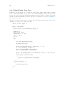
1
SICStus Prolog User’s Manual
by the Intelligent Systems Laboratory
Swedish Institute of Computer Science
PO Box 1263
SE-164 29 Kista, Sweden
Release 3.8.2
February 2000
Swedish Institute of Computer Science
[email protected]
http://www.sics.se/sicstus/
c 1995-2000 SICS
Copyright Swedish Institute of Computer Science
PO Box 1263
SE-164 29 Kista, Sweden
Permission is granted to make and distribute verbatim copies of this manual provided the
copyright notice and this permission notice are preserved on all copies.
Permission is granted to copy and distribute modified versions of this manual under the conditions for verbatim copying, provided that the entire resulting derived work is distributed
under the terms of a permission notice identical to this one.
Permission is granted to copy and distribute translations of this manual into another language, under the above conditions for modified versions, except that this permission notice
may be stated in a translation approved by SICS.
Introduction
1
Introduction
Prolog is a simple but powerful programming language developed at the University of Marseilles [Roussel 75], as a practical tool for programming in logic [Kowalski 74]. From a user’s
point of view the major attraction of the language is ease of programming. Clear, readable,
concise programs can be written quickly with few errors.
For an introduction to programming in Prolog, readers are recommended to consult [Sterling
& Shapiro 86]. However, for the benefit of those who do not have access to a copy of this
book, and for those who have some prior knowledge of logic programming, a summary of
the language is included. For a more general introduction to the field of Logic Programming
see [Kowalski 79]. See Chapter 3 [Prolog Intro], page 39.
This manual describes a Prolog system developed at the Swedish Institute of Computer
Science. Parts of the system were developed by the project “Industrialization of SICStus
Prolog” in collaboration with Ericsson Telecom AB, NobelTech Systems AB, Infologics AB
and Televerket. The system consists of a WAM emulator written in C, a library and runtime
system written in C and Prolog and an interpreter and a compiler written in Prolog. The
Prolog engine is a Warren Abstract Machine (WAM) emulator [Warren 83]. Two modes
of compilation are available: in-core i.e. incremental, and file-to-file. When compiled, a
predicate will run about 8 times faster and use memory more economically. Implementation
details can be found in [Carlsson 90] and in several technical reports available from SICS.
SICStus Prolog follows the mainstream Prolog tradition in terms of syntax and built-in
predicates, and is largely compatible with DECsystem-10 Prolog and Quintus Prolog.
2
SICStus Prolog
Acknowledgments
3
Acknowledgments
The following people have contributed to the development of SICStus Prolog:
Jonas Almgren, Johan Andersson, Stefan Andersson, Tamás Benkõ,
Kent Boortz, Per Brand, Göran Båge, Mats Carlsson, Jesper
Eskilson, Lena Flood, György Gyaraki, Seif Haridi, Ralph Haygood,
Christian Holzbaur, Key Hyckenberg, Per Mildner, Hans Nilsson, Mats
Nylén, Greger Ottosson, László Péter,
Dan Sahlin, Rob Scott, Thomas Sjöland, Péter
Szeredi, Johan Widén, and Emil Åström.
The Industrialization of SICStus Prolog (1988-1991) was funded by
Ericsson Telecom AB, NobelTech Systems AB, Infologics AB and
Televerket under the National Swedish Information Technology
Program IT4.
The development of release 3 (1991-1995) was funded in part by
Ellemtel Utvecklings AB
This manual is based on DECsystem-10 Prolog User’s Manual by
D.L. Bowen, L. Byrd, F.C.N. Pereira,
L.M. Pereira, D.H.D. Warren
See Chapter 31 [CLPQR], page 315, for acknowledgments relevant to the clp(Q,R) constraint
solver.
See Chapter 32 [CLPFD], page 339, for acknowledgments relevant to the clp(FD) constraint
solver.
UNIX is a trademark of Bell Laboratories. MSDOS and Windows is a trademark of Microsoft Corp. OS/2 is a trademark of IBM Corp.
4
SICStus Prolog
Notational Conventions
5
Notational Conventions
Keyboard Characters
When referring to keyboard characters, printing characters are written thus: a, while control
characters are written like this: ^A. Thus ^C is the character you get by holding down the
hCTLi key while you type c. Finally, the special control characters carriage-return, line-feed
and space are often abbreviated to hRETi, hLFDi and hSPCi respectively.
Mode Spec
When introducing a built-in predicate, we shall present its usage with a mode spec which
has the form name(arg, ..., arg) where each arg denotes how that argument should be
instantiated in goals, and has one of the following forms:
:ArgName This argument should be instantiated to a term denoting a goal or a clause or a
predicate name, or which otherwise needs special handling of module prefixes.
The argument is subject to module name expansion (see Section 4.5 [Meta Exp],
page 57).
+ArgName
This argument should be instantiated to a non-variable term.
-ArgName This argument should be uninstantiated.
?ArgName
This argument may or may not be instantiated.
Mode specs are not only used in the manual, but are part of the syntax of the language as
well. When used in the source code, however, the ArgName part must be omitted. That
is, arg must be either :, +, -, or ?.
Development and Runtime Systems
The full Prolog system with top-level, compiler, debugger etc. is known as the development
system.
It is possible to link user-written C code with a subset of SICStus Prolog to create runtime
systems. When introducing a built-in predicate, any limitations on its use in runtime
systems will be mentioned.
Function Prototypes
Whenever this manual documents a C function as part of SICStus Prolog’s foreign language
interface, the function prototype will be displayed in ANSI C syntax.
6
SICStus Prolog
ISO Compliance
SICStus Prolog provides two execution modes: the iso mode, which is fully compliant with
the International Standard ISO/IEC 13211-1 (PROLOG: Part 1—General Core), and the
sicstus mode, which supports code written in earlier versions of SICStus Prolog. The
execution mode can be changed using the Prolog flag language; see Section 7.6 [State Info],
page 137. Note, however, that SICStus Prolog does not offer a strictly conforming mode
which rejects uses of implementation specific features.
To aid programmers who wish to write standard compliant programs, built-in predicates
that are part of the ISO Prolog Standard are annotated with [ISO] in this manual. If such
a predicate behaves differently in sicstus mode, an appropriate clarification is given. For
the few predicates that have a completely different meaning in the two modes, two separate
descriptions are given. The one for the iso mode is annotated with [ISO only], while the
sicstus mode version is annotated with [SICStus only].
Chapter 1: Glossary
7
1 Glossary
abolish
To abolish a predicate is to retract all the predicate’s clauses and to remove
all information about it from the Prolog system, to make it as if that predicate
had never existed.
advice-point
A special case of breakpoint, the advice breakpoint. It is distinguished from
spypoints in that it is intended for non-interactive debugging, such as checking
of program invariants, collecting information, profiling, etc.
alphanumeric
An alphanumeric character is any of the lowercase characters from a to z, the
uppercase characters from A to Z, the numerals from 0 to 9, or underscore (_).
ancestors
An ancestor of a goal is any goal which the system is trying to solve when it
calls that goal. The most distant ancestor is the goal which was typed at the
top-level prompt.
anonymous
An anonymous variable is one which has no unique name, and whose value is
therefore inaccessible. An anonymous variable is denoted by an underscore (_).
argument
See predicate, structure, and arity.
arity
The arity of a structure is its number of arguments. For example, the structure
customer(jones,85) has an arity of 2.
atom
A character sequence used to uniquely denote some entity in the problem domain. A number is not an atom. Examples of legal atoms are:
hello
*
:=
’#$%’
’New York’
’don\’t’
See Section 3.1.1.3 [Atoms], page 40. Atoms are recognized by the built-in
predicate atom/1.
atomic term
Synonym for constant.
backtrace
A collection of information on the control flow of the program, gathered by the
debugger. Also the display of this information produced by the debugger. The
backtrace includes data on goals that were called but not exited and also on
goals that exited nondeterministically.
backtracking
The process of reviewing the goals that have been satisfied and attempting to
resatisfy these goals by finding alternative solutions.
binding
The process of assigning a value to a variable; used in unification.
blocked goal
A goal which is suspended because it is not instantiated enough.
body
The body of a clause consists of the part of a Prolog clause following the ‘:-’
symbol.
8
SICStus Prolog
breakpoint
A description of certain invocations in the program where the user wants the
debugger to stop, or to perform some other actions. A breakpoint is specific if
it applies to the calls of a specific predicate, possibly under some conditions,
otherwise it is generic. Depending on the intended usage, breakpoints can be
classified as debugger breakpoints, also known as spypoints, or advice breakpoints, also called advice-points; see Section 6.5 [Breakpoints], page 75.
buffer
A temporary workspace in Emacs that contains a file being edited.
built-in predicate
A predicate that comes with the system and which does not have to be explicitly
loaded before it is used.
callable term
A callable term is either a compound term or an atom. Callable terms are
recognized by the built-in predicate callable/1.
character code
An integer which is the numeric representation of a character. SICStus Prolog
supports character codes in the range 0..2147483647 (i.e. 2^31-1). However, to
be able to input or output character codes larger than 255, one needs to use
the appropriate wide character external encoding.
character code set
A subset of the set {0, ..., 2^31-1} that can be handled by the external encoding.
SICStus Prolog assumes that the character code set is an extension of the ASCII
code set, i.e. it includes codes 0..127, and these codes are interpreted as ASCII
characters
character-conversion mapping
SICStus Prolog maintains a character-conversion mapping which is used while
reading terms and programs. Initially, the mapping prescribes no character
conversions. It can be modified by the built-in predicate char_conversion(In,
Out), following which In will be converted to Out. Character coversion can be
switched off by the char_conversion Prolog flag.
character-type mapping
A function mapping each element of the character code set to one of the character categories (layout, letter, symbol-char, etc.), required for parsing tokens.
clause
A fact or a rule. A rule comprises a head and a body. A fact consists of a head
only, and is equivalent to a rule with the body true.
conjunction
A series of goals connected by the connective “and” (that is, a series of goals
whose principal operator is ‘,’).
compactcode
Virtual code representation of compiled code. A reasonable compromise between performance and space requirement. A valid value for the compiling
Prolog flag.
Chapter 1: Glossary
compile
9
To load a program (or a portion thereof) into Prolog through the compiler.
Compiled code runs more quickly than interpreted code, but you cannot debug
compiled code in as much detail as interpreted code.
compound term
A compound term is a functor together with zero or more arguments. For
example, in the term father(X), father/1 is the functor, and X is the first and
only argument. The argument to a compound term can be another compound
term, as in father(father(X)). Compound terms are recognized by the builtin predicate compound/1.
console-based executable
An executable which inherits the standard streams from the process that invoked it, e.g. a UNIX shell or a DOS-prompt.
constant
An integer (for example: 1, 20, -10), a floating-point number (for example: 12.35), or an atom. Constants are recognized by the built-in predicate
atomic/1.
consult
To load a program (or a portion thereof) into Prolog through the interpreter.
Interpreted code runs more slowly than compiled code, but you can debug
interpreted code in more detail than compiled code.
creep
What the debugger does in trace mode, also known as single-stepping. It goes
to the next port of a procedure box and prints the goal, then prompts you for
input. See Section 6.2 [Basic Debug], page 71.
cursor
The point on the screen at which typed characters appear. This is usually
highlighted by a line or rectangle the size of one space, which may or may not
blink.
cut
Written as !. A built-in predicate that succeeds when encountered; if backtracking should later return to the cut, the goal that matched the head of the
clause containing the cut fails immediately.
database
The Prolog database comprises all of the clauses which have been loaded or asserted into the Prolog system or which have been asserted, except those clauses
which have been retracted or abolished.
database reference
A compound term denoting a unique reference to a dynamic clause.
debug
A mode of program execution in which the debugger stops to print the current
goal only at procedures which have spypoints set on them (see leap).
debugcode
Interpreted representation of compiled code. A valid value for the compiling
Prolog flag.
declaration
A declaration looks like a directive, but is not executed but conveys information
about procedures about to be loaded.
deinit function
A function in a foreign resource which is called prior to unloading the resource.
10
SICStus Prolog
determinate
A procedure is determinate if it can supply only one answer.
development system
A stand-alone executable with the full programming environment, including
top-level, compiler, debugger etc. The default sicstus executable is a development system; new development systems containing pre-linked foreign resources
can also be created.
directive
A directive is a goal preceded by the prefix operator ‘:-’, whose intuitive meaning is “execute this as a query, but do not print out any variable bindings.”
disjunction
A series of goals connected by the connective “or” (that is, a series of goals
whose principal operator is ‘;’).
dynamic predicate
A predicate that can be modified while a program is running. A predicate must
explicitly be declared to be dynamic or it must be added to the database via
one of the assertion predicates.
encoded string
A sequence of bytes representing a sequence of possibly wide character codes,
using the UTF-8 encoding.
escape sequence
A sequence of characters beginning with \ inside certain syntactic tokens (see
[Escape Sequences], page 580).
export
A module exports a procedure so that other modules can import it.
external encoding (of wide characters)
A way of encoding sequences of wide characters as sequences of (8-bit) bytes,
used in stream input and output.
fact
A clause with no conditions—that is, with an empty body. A fact is a statement
that a relationship exists between its arguments. Some examples, with possible
interpretations, are:
king(louis, france).
% Louis was king of France.
have_beaks(birds).
% Birds have beaks.
employee(nancy, data_processing, 55000).
% Nancy is an employee in the
% data processing department.
fastcode
Native code representation of compiled code. The fastest, but also the most
space consuming representation. Only available for Sparc platforms. A valid
value for the compiling Prolog flag.
filename
An atom or a compound term denoting the name of a file. The rules for mapping
such terms to absolute filenames are described in Section 7.1 [Input Output],
page 98.
floundered query
A query where all unsolved goals are blocked.
Chapter 1: Glossary
11
foreign predicate
A predicate that is defined in a language other than Prolog, and explicitly
bound to Prolog predicates by the Foreign Language Interface.
foreign resource
A named set of foreign predicates.
functor
The name and arity of a compound term. For example, the compound term
foo(a,b) is said to have “the functor foo of arity two”, which is generally
written foo/2.
garbage collection
The freeing up of space for computation by making the space occupied by terms
which are no longer available for use by the Prolog system.
generalized predicate spec
A generalized predicate spec is a term of one of the following forms. It is always
interpreted wrt. a given module context:
Name
all predicates called Name no matter what arity, where Name is an
atom for a specific name or a variable for all names, or
Name/Arity
the predicate of that name and arity, or
Name/(Low-High)
Name/[Low-High]
the predicates of that name with arity in the range Low-High, or
Name/[Arity,...,Arity]
the predicates of that name with one of the given arities, or
Module:Spec
specifying a particular module Module instead of the default module, where Module is an atom for a specific module or a variable
for all modules, or
[Spec,...,Spec]
the set of all predicates covered by the Specs.
glue code
Interface code between the Prolog engine and foreign predicates. Automatically
generated by the foreign language interface as part of building a linked foreign
resource.
goal
A simple goal is a predicate call. When called, it will either succeed or fail.
A compound goal is a formula consisting of simple goals connected by connectives such as “and” (‘,’) or “or” (‘;’).
A goal typed at the top level is called a query.
ground
A term is ground when it is free of (unbound) variables. Ground terms are
recognized by the built-in predicate ground/1.
head
The head of a clause is the single goal which will be satisfied if the conditions
in the body (if any) are true; the part of a rule before the ‘:-’ symbol. The
head of a list is the first element of the list.
12
SICStus Prolog
hook predicate
A hook predicate is a procedure that somehow alters or customizes the behavior
of a hookable predicate.
hookable predicate
A hookable predicate is a built-in predicate whose behavior is somehow altered
or customized by a hook predicate.
import
Exported procedures in a module can be imported by other modules. Once a
procedure has been imported by a module, it can be called, or exported, as if
it were defined in that module.
There are two kinds of importation: procedure-importation, in which only specified procedures are imported from a module; and module-importation, in which
all the predicates made exported by a module are imported.
indexing
The process of filtering a set of potentially matching clauses of a procedure given
a goal. For interpreted and compiled code, indexing is done on the principal
functor of the first argument. Indexing is coarse w.r.t. big integers and floats.
init function
A function in a foreign resource which is called upon loading the resource.
initialization
An initialization is a goal that is executed when the file in which the initialization is declared is loaded, or upon reinitialization. A initialization is declared
as a directive :- initialization Goal.
instantiation
A variable is instantiated if it is bound to a non-variable term; that is, to an
atomic term or a compound term.
internal encoding (of wide characters)
A way of encoding wide character sequences internally within the Prolog system.
SICStus Prolog uses a technique known as the UTF-8 encoding for this purpose.
interpret
Load a program or set of clauses into Prolog through the interpreter (also
known as consulting). Interpreted code runs more slowly than compiled code,
but more extensive facilities are available for debugging interpreted code.
invocation box
Same as procedure box.
leap
What the debugger does in debug mode. The debugger shows only the ports
of procedures that have spypoints on them. It then normally prompts you for
input, at which time you may leap again to the next spypoint (see trace).
leashing
Determines how frequently the debugger will stop and prompt you for input
when you are tracing. A port at which the debugger stops is called a “leashed
port”.
linked foreign resource
A foreign resource that is ready to be installed in an atomic operation, normally
represented as a shared object or DLL.
Chapter 1: Glossary
13
list
A list is written as a set of zero or more terms between square brackets. If there
are no terms in a list, it is said to be empty, and is written as []. In this first
set of examples, all members of each list are explicitly stated:
[aa, bb,cc] [X, Y] [Name] [[x, y], z]
In the second set of examples, only the first several members of each list are
explicitly stated, while the rest of the list is represented by a variable on the
right-hand side of the “rest of” operator, |:
[X | Y] [a, b, c | Y] [[x, y] | Rest]
| is also known as the “list constructor.” The first element of the list to the
left of | is called the head of the list. The rest of the list, including the variable
following | (which represents a list of any length), is called the tail of the list.
load
To load a Prolog clause or set of clauses, in source or binary form, from a file
or set of files.
meta-call
The process of interpreting a callable term as a goal. This is done e.g. by the
built-in predicate call/1.
meta-predicate
A meta-predicate is one which calls one or more of its arguments; more generally, any predicate which needs to assume some module in order to operate
is called a meta-predicate. Some arguments of a meta-predicate are subject to
module name expansion.
mode spec
A term name(arg, ..., arg) where each arg denotes how that argument should
be instantiated in goals. See [Mode Spec], page 5.
module
A module is a set of procedures in a module-file. Some procedures in a module
are exported. The default module is user.
module name expansion
The process by which certain arguments of meta-predicates get prefixed by the
source module. See Section 4.5 [Meta Exp], page 57.
module-file
A module-file is a file that is headed with a module declaration of the form"
:- module(ModuleName, ExportedPredList).
which must appear as the first term in the file.
multifile predicate
A predicate whose definition is to be spread over more than one file. Such
a predicate must be preceded by an explicit multifile declaration in all files
containing clauses for it.
mutable term
A special form of compound term which is subject to destructive assignment.
See Section 7.8 [Modify Term], page 149. Mutable terms are recognized by the
built-in predicate is_mutable/1.
name clash
A name clash occurs when a module attempts to define or import a procedure
that it has already defined or imported.
14
SICStus Prolog
occurs-check
A test to ensure that binding a variable does not bind it to a term where that
variable occurs.
one-char atom
An atom which consists of a single character.
operator
A notational convenience that allows you to express any compound term in a
different format. For example, if likes in
| ?- likes(sue, cider).
is declared an infix operator, the query above could be written:
| ?- sue likes cider.
An operator does not have to be associated with a predicate. However, certain
built-in predicates are declared as operators. For example,
| ?- =..(X, Y).
can be written as
| ?- X =.. Y.
because =.. has been declared an infix operator.
Those predicates which correspond to built-in operators are written using infix
notation in the list of built-in predicates at the beginning of the part that
contains the reference pages.
Some built-in operators do not correspond to built-in predicates; for example,
arithmetic operators. See [Standard Operators], page 583 for a list of built-in
operators.
pair
A compound term K-V . Pairs are used by the built-in predicate keysort/2
and by many library modules.
parent
The parent of the current goal is a goal which, in its attempt to obtain a
successful solution to itself, is calling the current goal.
port
One of the five key points of interest in the execution of a Prolog procedure.
See Section 6.1 [Procedure Box], page 69 for a definition.
pre-linked foreign resource
A linked foreign resource that is linked into a stand-alone executable as part of
building the executable.
precedence
A number associated with each Prolog operator, which is used to disambiguate
the structure of the term represented by an expression containing a number
of operators. Operators of lower precedence are applied before those of higher
precedence; the operator with the highest precedence is considered the principal
functor of the expression. To disambiguate operators of the same precedence,
the associativity type is also necessary. See Section 3.6 [Operators], page 49.
predicate
A functor that specifies some relationship existing in the problem domain. For
example, < /2 is a built-in predicate specifying the relationship of one number
being less than another. In contrast, the functor + /2 is not (normally used as)
a predicate.
Chapter 1: Glossary
15
A predicate is either built-in or is implemented by a procedure.
predicate spec
A compound term name/arity or module:name/arity denoting a predicate.
procedure A set of clauses in which the head of each clause has the same predicate. For
instance, a group of clauses of the following form:
connects(san_francisco, oakland, bart_train).
connects(san_francisco, fremont, bart_train).
connects(concord, daly_city, bart_train).
is identified as belonging to the procedure connects/3.
procedure box
A way of visualizing the execution of a Prolog procedure, A procedure box is
entered and exited via ports.
profiledcode
Virtual code representation of compiled code, instrumented for profiling. A
valid value for the compiling Prolog flag.
profiling
The process of gathering execution statistics of parts of the program, essentially
counting the times selected program points have been reached.
program
A set of procedures designed to perform a given task.
PO file
A PO (Prolog object) file contains a binary representation of a set of modules, predicates, clauses and directives. They are portable between different
platforms, except between 32-bit and 64-bit platforms. They are created by
save_files/2, save_modules/2, and save_predicates/2.
QL file
A QL (quick load) file contains an intermediate representation of a compiled
source code file. They are portable between different platforms, but less efficient
than PO files, and are therefore obsolescent. They are created by fcompile/1.
query
A query is a question put by the user to the Prolog system. A query is written
as a goal followed by a full-stop in response to the Prolog system prompt. For
example,
| ?- father(edward, ralph).
refers to the predicate father/2. If a query has no variables in it, the system
will respond either ‘yes’ or ‘no’. If a query contains variables, the system will
try to find values of those variables for which the query is true. For example,
| ?- father(edward, X).
X = ralph
After the system has found one answer, the user can direct the system to look
for additional answers to the query by typing ‘;’.
recursion
The process in which a running procedure calls itself, presumably with different
arguments and for the purpose of solving some subset of the original problem.
region
The text between the cursor and a previously set mark in an Emacs buffer.
rule
A clause with one or more conditions. For a rule to be true, all of its conditions
must also be true. For example,
16
SICStus Prolog
has_stiff_neck(ralph) :hacker(ralph).
This rule states that if the individual ralph is a hacker, then he must also have
a stiff neck. The constant ralph is replaced in
has_stiff_neck(X) :hacker(X).
by the variable X. X unifies with anything, so this rule can be used to prove
that any hacker has a stiff neck.
runtime kernel
A shared object or DLL containing the SICStus virtual machine and other
runtime support for stand-alone executables.
runtime system
A stand-alone executable with a restricted set of built-in predicates and no toplevel. Stand-alone applications containing debugged Prolog code and destined
for end-users are typically packaged as runtime systems.
saved-state
A snapshot of the state of Prolog saved in a file by save_program/[1,2].
semantics
The relation between the set of Prolog symbols and their combinations (as
Prolog terms and clauses), and their meanings. Compare syntax.
sentence
A clause or directive.
side-effect A predicate which produces a side-effect is one which has any effect on the
“outside world” (the user’s terminal, a file, etc.), or which changes the Prolog
database.
simple term
A simple term is a constant or a variable. Simple terms are recognized by the
built-in predicate simple/1.
source code
The human-readable, as opposed to the machine-executable, representation of
a program.
source module
The module which is the context of a file being loaded. For module-files, the
source module is named in the file’s module declaration. For other files, the
source module is inherited from the context.
SP term ref
A “handle” object providing an interface from C to Prolog terms.
spypoint
A special case of breakpoint, the debugger breakpoint, intended for interactive
debugging. Its simplest form, the plain spypoint instructs the debugger to stop
at all ports of all invocations of a specified predicate. Conditional spypoints
apply to a single predicate, but are more selective: the user can supply applicability tests and prescribe the actions to be carried out by the debugger. A
generic spypoint is like a conditional spypoint, but not restricted to a single
predicate. See Section 6.5 [Breakpoints], page 75.
Chapter 1: Glossary
17
stand-alone executable
A binary program which can be invoked from the operating system, containing
the SICStus runtime kernel. A stand-alone executable is a development system
(e.g. the default sicstus executable), or a runtime system. Both kinds are
created by the spld utility. A stand-alone executable does not itself contain
any Prolog code; all Prolog code must be loaded upon startup.
static predicate
A predicate that can be modified only by being reloaded or by being abolished.
See dynamic predicate.
stream
An input/output channel. See Section 7.1 [Input Output], page 98.
stream alias
A name assigned to a stream at the time of opening, which can be referred to
in I/O predicates. Must be an atom. There are also three predefined aliases for
the standard streams: user_input, user_output and user_error.
string
A special syntactic notation which is, by default, equivalent to a list of character
codes e.g.
"SICStus"
By setting the Prolog flag double_quotes, the meaning of strings can be
changed. With an appropriate setting, a string can be made equivalent to
a list of one-char atoms, or to an atom. Strings are not a separate data type.
subterm selector
A list of argument positions selecting a subterm within a term (i.e. the subterm
can be reached from the term by successively selecting the argument positions
listed in the selector). Example: within the term q, (r, s; t) the subterm s
is selected by the selector [2, 1, 2].
syntax
The part of Prolog grammar dealing with the way in which symbols are put
together to form legal Prolog terms. Compare semantics.
system encoding (of wide characters)
A way of encoding wide character strings, used or required by the operating
system environment.
term
A basic data object in Prolog. A term can be a constant, a variable, or a
compound term.
trace
A mode of program execution in which the debugger creeps to the next port
and prints the goal.
type-in module
The module which is the context of queries.
unblocked goal
A goal which is not blocked.
unbound
A variable is unbound if it has not yet been instantiated.
unification The process of matching a goal with the head of a clause during the evaluation
of a query, or of matching arbitrary terms with one another during program
execution.
18
SICStus Prolog
The rules governing the unification of terms are:
• Two constants unify with one another if they are identical.
• A variable unifies with a constant or a compound term. As a result of the
unification, the variable is instantiated to the constant or compound term.
• A variable unifies with another variable. As a result of the unification, they
become the same variable.
• A compound term unifies with another compound term if they have the
same functor and if all of the arguments can be unified.
unit clause
See fact.
UTF-8 encoding
See internal encoding
variable
A logical variable is a name that stands for objects that may or may not be
determined at a specific point in a Prolog program. When the object for which
the variable stands is determined in the Prolog program, the variable becomes
instantiated. A logical variable may be unified with a constant, a compound
term, or another variable. Variables become uninstantiated when the procedure
they occur in backtracks past the point at which they were instantiated.
Variables may be written as any sequence of alphanumeric characters starting
with either a capital letter or _; e.g.
X
Y
Z
Name
Position
_c
_305 One_stop
See Section 3.1.1.4 [Variables], page 40.
volatile
Predicate property. The clauses of a volatile predicate are not saved in savedstates.
windowed executable
An executable which pops up its own window when run, and which directs the
standard streams to that window.
zip
Same as leap mode, except no debugging information is collected while zipping.
Chapter 2: How to Run Prolog
19
2 How to Run Prolog
SICStus Prolog offers the user an interactive programming environment with tools for incrementally building programs, debugging programs by following their executions, and modifying parts of programs without having to start again from scratch.
The text of a Prolog program is normally created in a file or a number of files using one of
the standard text editors. The Prolog interpreter can then be instructed to read in programs
from these files; this is called consulting the file. Alternatively, the Prolog compiler can be
used for compiling the file.
2.1 Getting Started
Under UNIX, SICStus Prolog is normally started from one of the shells. On other platforms,
it is normally started by clicking on an icon. However, it is often convenient to run SICStus
Prolog under GNU Emacs instead. A GNU Emacs interface for SICStus Prolog is described
later (see Section 2.11 [Emacs Interface], page 29). From a shell, SICStus Prolog is started
by typing:
% sicstus [options] [-a argument...]
where flags have the following meaning:
-f
Fast start.
Don’t read any initialization file (‘~/.sicstusrc’ or
‘~/.sicstus.ini’) on startup. If the flag is omitted and this file exists, SICStus
Prolog will consult it on startup after running any initializations and printing
the version banners.
-i
Forced interactive. Prompt for user input, even if the standard input stream
does not appear to be a terminal.
-m
Use malloc()/free() in the memory manager’s bottom layer.
-l prolog-file
Ensure that the file prolog-file is loaded on startup. This is done before any
initialization file is loaded.
-r saved-state
Restore the saved state saved-state on startup. This is done before any prologfile or initialization file is loaded.
-a argument...
where the arguments can be retrieved from Prolog by prolog_flag(argv,
Args), which will unify Args with argument... represented as a list of atoms.
-B[abspath]
Creates a saved state for a development system. This option is not needed
for normal use. If abspath is given, it specifies the absolute pathname for the
saved state. NOTE: There must not be a space before the path, or it will be
interpreted as a separate option.
20
SICStus Prolog
-R[abspath]
Equivalent to the -B option, except that it builds a saved state for a runtime
system instead.
Under UNIX, a saved state file can be executed directly by typing:
% file argument...
This is equivalent to:
% sicstus -r file [-a argument...]
NOTE: As of release 3.7, saved-states do not store the complete path of the binary sp.exe.
Instead, they call the main executable sicstus, which is assumed to be found in the shell’s
path. If there are several versions of SICStus installed, it is up to the user to make sure
that the correct start-script is found.
Notice that the flags are not available when executing saved states—all the command-line
arguments are treated as Prolog arguments.
The development system checks that a valid SICStus license exists and responds with a
message of identification and the prompt ‘| ?- ’ as soon as it is ready to accept input,
thus:
SICStus 3.8.2 (sparc-solaris-5.7): Thu Aug 19 16:25:28 MET DST 1999
Licensed to SICS
| ?At this point the top-level is expecting input of a query. You cannot type in clauses or
directives immediately (see Section 2.3 [Inserting Clauses], page 22). While typing in a
query, the prompt (on following lines) becomes ‘
’. That is, the ‘| ?- ’ appears only
for the first line of the query, and subsequent lines are indented.
2.1.1 Environment Variables
The following environment variables can be set before starting SICStus Prolog. Some of
these override the default sizes of certain areas. The sizes are given in bytes, but may be
followed by K or M meaning kilobytes or megabytes respectively.
SP_CSETLEN
Selects the sub-code-set lengths when the EUC character set is used. For the
details, see Section 10.4 [WCX Environment Variables], page 225.
SP_CTYPE
Selects the appropriate character set standard: The supported values are euc
(for EUC), utf8 (for Unicode) and iso_8859_1 (for ISO 8859/1). The latter
is the default. For the details, see Section 10.4 [WCX Environment Variables],
page 225.
SP_PATH
This environment variable can be used to specify the location of the Runtime
Library (corresponding to the third argument to SP_initialize()). See sec-
Chapter 2: How to Run Prolog
21
tion “Setting SP PATH under UNIX” in SICStus Prolog Release Notes, for
more information.
TMPDIR
If set, indicates the pathname where temporary files should be created. Defaults
to ‘/usr/tmp’.
GLOBALSTKSIZE
Governs the initial size of the global stack.
LOCALSTKSIZE
Governs the initial size of the local stack.
CHOICESTKSIZE
Governs the initial size of the choicepoint stack.
TRAILSTKSIZE
Governs the initial size of the trail stack.
PROLOGINITSIZE
Governs the size of Prolog’s initial memory allocation.
PROLOGMAXSIZE
Defines a limit on the amount of data space which Prolog will use.
PROLOGINCSIZE
Governs the amount of space Prolog asks the operating system for in any given
memory expansion.
PROLOGKEEPSIZE
Governs the size of space Prolog retains after performing some computation.
By default, Prolog gets memory from the operating system as the user program
executes and returns all free memory back to the operating system when the
user program does not need any more. If the programmer knows that her
program, once it has grown to a certain size, is likely to need as much memory
for future computations, then she can advise Prolog not to return all the free
memory back to the operating system by setting this variable. Only memory
that is allocated above and beyond PROLOGKEEPSIZE is returned to the OS; the
rest will be kept.
Send bug reports to [email protected]. Bugs tend actually to be fixed if they can
be isolated, so it is in your interest to report them in such a way that they can be easily
reproduced.
The
mailing
list
[email protected]
is
a
moderated
mailing list for communication among users and implementors. To [un]subscribe, write
to [email protected].
2.2 Reading in Programs
A program is made up of a sequence of clauses and directives. The clauses of a predicate
do not have to be immediately consecutive, but remember that their relative order may be
important (see Section 3.3 [Procedural], page 45).
22
SICStus Prolog
To input a program from a file file, just type the filename inside list brackets (followed by
. and hRETi), thus:
| ?- [file].
This instructs the interpreter to read in (consult) the program. Note that it may be necessary to enclose the filename file in single quotes to make it a legal Prolog atom; e.g.
| ?- [’myfile.pl’].
| ?- [’/usr/prolog/somefile’].
The specified file is then read in. Clauses in the file are stored so that they can later be
interpreted, while any directives are obeyed as they are encountered. When the end of
the file is found, the system displays on the standard error stream the time spent. This
indicates the completion of the query.
Predicates that expect the name of a Prolog source file as an argument use absolute_
file_name/2 (see Section 7.1.5 [Stream Pred], page 118) to look up the file. If no explicit
extension is given, this predicate will look for a file with the default extension ‘.pl’ added
as well as for a file without extension. There is also support for libraries.
In general, this query can be any list of filenames, such as:
| ?- [myprog,extras,tests].
In this case all three files would be consulted.
The clauses for all the predicates in the consulted files will replace any existing clauses for
those predicates, i.e. any such previously existing clauses in the database will be deleted.
Note that consult/1 in SICStus Prolog behaves like reconsult/1 in DEC-10 Prolog.
2.3 Inserting Clauses at the Terminal
Clauses may also be typed in directly at the terminal, although this is only recommended
if the clauses will not be needed permanently, and are few in number. To enter clauses at
the terminal, you must give the special query:
| ?- [user].
|
and the new prompt ‘| ’ shows that the system is now in a state where it expects input of
clauses or directives. To return to top level, type ^D. The system responds thus:
{user consulted, 20 msec 200 bytes}
Chapter 2: How to Run Prolog
23
2.4 Queries and Directives
Queries and directives are ways of directing the system to execute some goal or goals.
In the following, suppose that list membership has been defined by loading the following
clauses from a file:
member(X, [X|_]).
member(X, [_|L]) :- member(X, L).
(Notice the use of anonymous variables written ‘_’.)
2.4.1 Queries
The full syntax of a query is ‘?-’ followed by a sequence of goals. The top level expects
queries. This is signaled by the initial prompt ‘| ?- ’. Thus a query at top level looks like:
| ?- member(b, [a,b,c]).
Remember that Prolog terms must terminate with a full stop (., possibly followed by layout
text), and that therefore Prolog will not execute anything until you have typed the full stop
(and then hRETi) at the end of the query.
If the goal(s) specified in a query can be satisfied, and if there are no variables as in this
example, then the system answers
yes
and execution of the query terminates.
If variables are included in the query, then the final value of each variable is displayed
(except for variables whose names begin with _). Thus the query
| ?- member(X, [a,b,c]).
would be answered by
X = a
At this point the system is waiting for input of either just a hRETi or else a ; followed by
hRETi. Simply typing hRETi terminates the query; the system responds with ‘yes’. However,
typing ; causes the system to backtrack (see Section 3.3 [Procedural], page 45) looking for
alternative solutions. If no further solutions can be found it outputs ‘no’.
The outcome of some queries is shown below, where a number preceded by _ is a systemgenerated name for a variable.
| ?- member(X, [tom,dick,harry]).
X = tom ;
X = dick ;
24
SICStus Prolog
X = harry ;
no
| ?- member(X, [a,b,f(Y,c)]), member(X, [f(b,Z),d]).
X = f(b,c),
Y = b,
Z = c
yes
| ?- member(X, [f(_),g]).
X = f(_A)
yes
| ?Directives are like queries except that:
1. Variable bindings are not displayed if and when the directive succeeds.
2. You are not given the chance to backtrack through other solutions.
2.4.2 Directives
Directives start with the symbol ‘:-’. Any required output must be programmed explicitly;
e.g. the directive:
:- member(3, [1,2,3]), write(ok).
asks the system to check whether 3 belongs to the list [1,2,3]. Execution of a directive terminates when all the goals in the directive have been successfully executed. Other
alternative solutions are not sought. If no solution can be found, the system prints:
{Warning: Goal - goal failed}
as a warning.
The principal use for directives (as opposed to queries) is to allow files to contain directives
which call various predicates, but for which you do not want to have the answers printed
out. In such cases you only want to call the predicates for their effect, i.e. you don’t want
terminal interaction in the middle of consulting the file. A useful example would be the use
of a directive in a file which consults a whole list of other files, e.g.
:- [ bits, bobs, main, tests, data, junk ].
If a directive like this were contained in the file ‘myprog’ then typing the following at toplevel would be a quick way of reading in your entire program:
| ?- [myprog].
Chapter 2: How to Run Prolog
25
When simply interacting with the top-level, this distinction between queries and directives
is not normally very important. At top-level you should just type queries normally. In a
file, queries are in fact treated as directives, i.e. if you wish to execute some goals then the
directive in the file must be preceded by ‘:-’ or ‘?-’, otherwise it would be treated as a
clause.
2.5 Syntax Errors
Syntax errors are detected during reading. Each clause, directive or in general any term
read in by the built-in predicate read/1 that fails to comply with syntax requirements is
displayed on the standard error stream as soon as it is read, along with its position in the
input stream and a mark indicating the point in the string of symbols where the parser has
failed to continue analysis, e.g.:
| member(X, X$L).
{SYNTAX ERROR: in line 5 (within 5-6)}
** , or ) expected in arguments **
member ( X , X
** here **
$ L ) .
if $ has not been declared as an infix operator.
Note that any comments in the faulty line are not displayed with the error message. If you
are in doubt about which clause was wrong you can use the listing/1 predicate to list all
the clauses which were successfully read in, e.g.
| ?- listing(member/2).
NOTE: The built in predicates read/[1,2] normaly raise an exception on syntax errors (see
Section 7.5 [Exception], page 134). The behavior is controlled by the flag syntax_errors
(see prolog_flag/3).
2.6 Undefined Predicates
There is a difference between predicates that have no definition and predicates that have
no clauses. The latter case is meaningful e.g. for dynamic predicates (see Section 5.2
[Declarations], page 62) that clauses are being added to or removed from. There are good
reasons for treating calls to undefined predicates as errors, as such calls easily arise from
typing errors.
The system can optionally catch calls to predicates that have no definition. First the
user defined predicate user:unknown_predicate_handler/3 (see Section 7.5 [Exception],
page 134) is called. If undefined or if the call fails the action is governed by the state of the
unknown/2 flag which can be:
26
SICStus Prolog
trace
which causes calls to undefined predicates to be reported and the debugger to
be entered at the earliest opportunity.
error
which causes calls to such predicates to raise an exception (the default state).
See Section 7.5 [Exception], page 134.
warning
which causes calls to such predicates to display a warning message and then
fail.
fail
which causes calls to such predicates to fail.
Calls to predicates that have no clauses are not caught.
The built-in predicate unknown(?OldState, ?NewState) unifies OldState with the current
state and sets the state to NewState. The built-in predicate debugging/0 prints the value of
this state along with its other information. This state is also controlled by the flag unknown
(see prolog_flag/3).
2.7 Program Execution And Interruption
Execution of a program is started by giving the system a query which contains a call to one
of the program’s predicates.
Only when execution of one query is complete does the system become ready for another
query. However, one may interrupt the normal execution of a query by typing ^C. This
^C interruption has the effect of suspending the execution, and the following message is
displayed:
Prolog interruption (h or ? for help) ?
At this point, the development system accepts one-letter commands corresponding to certain
actions. To execute an action simply type the corresponding character (lower or upper case)
followed by hRETi. The available commands in development systems are:
a
aborts the current computation.
c
continues the execution.
e
exits from SICStus Prolog, closing all files.
h
?
lists available commands.
b
invokes a recursive top-level.
d
z
t
switch on the debugger. See Chapter 6 [Debug Intro], page 69.
If the standard input stream is not connected to the terminal, e.g. by redirecting standard
input to a file or a pipe, the above ^C interrupt options are not available. Instead, typing
^C causes SICStus Prolog to exit, and no terminal prompts are printed.
Chapter 2: How to Run Prolog
27
2.8 Exiting From The Top-Level
To exit from the top-level and return to the shell, either type ^D at the top-level, or call the
built-in predicate halt/0, or use the e (exit) command following a ^C interruption.
2.9 Nested Executions—Break and Abort
The Prolog system provides a way to suspend the execution of your program and to enter
a new incarnation of the top level where you can issue queries to solve goals etc. This is
achieved by issuing the query (see Section 2.7 [Execution], page 26):
| ?- break.
This invokes a recursive top-level, indicated by the message:
{ Break level 1 }
You can now type queries just as if you were at top-level.
If another call of break/0 is encountered, it moves up to level 2, and so on. To close the
break and resume the execution which was suspended, type ^D. The debugger state and
current input and output streams will be restored, and execution will be resumed at the
predicate call where it had been suspended after printing the message:
{ End break }
Alternatively, the suspended execution can be aborted by calling the built-in predicate
abort/0.
A suspended execution can be aborted by issuing the query:
| ?- abort.
within a break. In this case no ^D is needed to close the break; all break levels are discarded
and the system returns right back to top-level. I/O streams remain open, but the debugger
is switched off. abort/0 may also be called from within a program.
2.10 Saving and Restoring Program States
Once a program has been read, the system will have available all the information necessary
for its execution. This information is called a program state.
The state of a program may be saved on disk for future execution. The state consists
of all predicates and modules except built-in predicates and clauses of volatile predicates,
the current operator declarations, the values of all writable Prolog flags except debugging,
source_info, and the user_* stream aliases (see Section 7.6 [State Info], page 137), any
blackboard data (see Section 7.11 [Blackboard Primitives], page 152), internal database
data (see Section 7.10 [Database], page 152), and profiling data (see Section 7.15 [Profiling],
page 158), but no information for source-linked debugging.
28
SICStus Prolog
To save a program into a file File, type the following query. On UNIX platforms, the file
becomes executable:
| ?- save_program(File).
You can also specify a goal to be run when a saved program is restored. This is done by:
| ?- save_program(File, start).
where start/0 is the predicate to be called.
Once a program has been saved into a file File, the following query will restore the system
to the saved state:
| ?- restore(File).
If a saved state has been moved or copied to another machine, the path names of foreign
resources and other files needed upon restore are typically different at restore time from
their save time values. To solve this problem, certain atoms will be relocated during restore
as follows:
• Atoms that had ‘$SP_PATH/library’ (the name of the directory containing the Prolog
Library) as prefix at save time will have that prefix replaced by the corresponding
restore time value.
• Atoms that had the name of the directory containing File as prefix at save time will
have that prefix replaced by the corresponding restore time value.
The purpose of this procedure is to be able to build and deploy an application consisting of
a saved state and other files as a directory tree with the saved state at the root: as long as
the other files maintain their relative position in the deployed copy, they can still be found
upon restore.
NOTE: Foreign resources, see Section 8.2 [Calling C], page 166, are unloaded by save_
program/[1,2]. The names and paths of the resources, typically ‘$SP_PATH/library’
relative, are however included in the saved state. After the save, and after restoring a
saved state, this information is used to reload the foreign resources again. The state of the
foreign resource in terms of global C variables and allocated memory is thus not preserved.
Foreign resources may define init and deinit functions to take special action upon loading
and unloading, see Section 8.2.6 [Init and Deinit Functions], page 173.
As of SICStus Prolog 3.8, partial saved states corresponding to a set of source files, modules,
and predicates can be created by the built-in predicates save_files/2, save_modules/2,
and save_predicates/2 respectively. These predicates create files in a binary format,
by default with the prefix ‘.po’ (for Prolog object file), which can be loaded by load_
files/[1,2]. For example, to compile a program split into several source files into a single
object file, type:
| ?- compile(Files), save_files(Files, Object).
Chapter 2: How to Run Prolog
29
For each filename given, the first goal will try to locate a source file with the default suffix
‘.pl’ and compile it into memory. The second goal will save the program just compiled
into an object file whose default suffix is ‘.po’. Thus the object file will contain a partial
memory image.
2.11 Emacs Interface
This section explains how to use the GNU Emacs interface for SICStus Prolog, and how to
customize your GNU Emacs environment for it.
Emacs is a powerful programmable editor especially suitable for program development. It
is available for free for many platforms, including various UNIX dialects, Windows and
MacOS. For information on obtaining Emacs, see www.emacs.org. For information specific
to GNU Emacs or XEmacs, see www.gnu.org and www.xemacs.org respectively.
The advantages of using SICStus in the Emacs environment are source-linked debugging,
auto indentation, syntax highlighting, help on predefined predicates (requires the SICStus
info files to be installed), loading code from inside Emacs, auto-fill mode, and more.
The Emacs interface is not part of SICStus Prolog proper, but is included in the distribution
for convenience. It was written by Emil Åström and Milan Zamazal, based on an earlier
version of the mode written by Masanobu Umeda. Contributions has also been made by
Johan Andersson, Peter Olin, Mats Carlsson, Johan Bevemyr, Stefan Andersson, and Per
Danielsson, Henrik Båkman, and Tamás Rozmán. Some ideas and also a few lines of code
have been borrowed (with permission) from Oz.el by Ralf Scheidhauer and Michael Mehl,
the Emacs major mode for the Oz programming language. More ideas and code have been
taken from the SICStus debugger mode by Per Mildner.
2.11.1 Installation
See section “The Emacs Interface” in SICStus Prolog Release Notes, for more information
about installing the Emacs interface.
There are some differences between GNU Emacs and XEmacs. This will be indicated with
Emacs-Lisp comments in the examples.
2.11.1.1 Customizing Emacs
Version 20 of GNU Emacs and XEmacs introduced a new method for editing and storing
user settings. This feature is available from the menu bar as ‘Customize’ and particular
Emacs variables can be customized with M-x customize-variable. Using ‘Customize’ is
the preferred way to modify the settings for emacs and the appropriate customize commands
will be indicated below, sometimes together with the old method of directly setting Emacs
variables.
30
SICStus Prolog
2.11.1.2 Enabling Emacs Support for SICStus
Assuming the Emacs interface for SICStus Prolog has been installed in the default location,
inserting the following lines in your ‘~/.emacs’ will make Emacs use this mode automatically
when editing files with a ‘.pl’ extension:
(setq load-path
(cons (expand-file-name "/usr/local/lib/sicstus-3.8/emacs")
load-path))
(autoload ’run-prolog "prolog" "Start a Prolog sub-process." t)
(autoload ’prolog-mode "prolog" "Major mode for editing Prolog programs." t)
(setq prolog-use-sicstus-sd t)
(setq auto-mode-alist (cons ’("\\.pl$" . prolog-mode) auto-mode-alist))
where the path in the first line is the file system path to ‘prolog.el’ (the generic Prolog
mode) and ‘sicstus-support.el’ (SICStus specific code). For example, ‘~/emacs’ means
that the file is in the user’s home directory, in directory emacs. Windows paths can be
written like ‘C:/Program Files/SICStus/emacs’.
The last line above makes sure that files ending with ‘.pl’ are assumed to be Prolog files
and not Perl, which is the default Emacs setting. If this is undesirable, remove that line.
It is then necessary for the user to manually switch to prolog mode by typing M-x prologmode after opening a prolog file, for an alternative approach, see Section 2.11.4 [Mode Line],
page 33.
If the shell command sicstus is not available in the default path, then it is necessary to
set the value of the environment variable EPROLOG to a shell command to invoke SICStus
Prolog. This is an example for C Shell:
setenv EPROLOG /usr/local/bin/sicstus
2.11.1.3 Enabling Emacs Support for SICStus Documentation
It is possible to look up the documentation for any built in or library predicate from within
Emacs (using C-c ? or the menu). For this to work Emacs must be told about the location
of the ‘info’-files that make up the documentation.
The default location for the ‘info’-files are ‘<prefix>/lib/sicstus-3.8/doc/info/’ on
UNIX platforms and ‘C:/Program Files/SICStus/doc/info/’ on Windows.
Add the following to your ‘~/.emacs’ file, assuming INFO is the path to the info files, e.g.,
‘C:/Program Files/SICStus/doc/info/’
(setq Info-default-directory-list
(append Info-default-directory-list ’("INFO")))
for GNU Emacs, or
(setq Info-directory-list
(append Info-directory-list ’("INFO")))
Chapter 2: How to Run Prolog
31
for XEmacs. You can also use M-x customize-group hRETi info hRETi if your Emacs is new
enough. You may have to quit and restart Emacs for these changes to take effect.
2.11.2 Basic Configuration
If the following lines are not present in ‘~/.emacs’, we suggest they are added, so that
the font-lock mode (syntax coloring support) is enabled for all major modes in Emacs that
support it.
(global-font-lock-mode t)
; GNU Emacs
(setq font-lock-auto-fontify t) ; XEmacs
(setq font-lock-maximum-decoration t)
These settings and more are also available through M-x customize-group hRETi font-lock.
If one wants to add font-locking only to the prolog mode, the two lines above could be
replaced by:
(add-hook ’prolog-mode-hook ’turn-on-font-lock)
Similarly, to turn it off only for prolog mode use:
(add-hook ’prolog-mode-hook ’turn-off-font-lock)
2.11.3 Usage
A prolog process can be started by choosing Run Prolog from the Prolog menu, by typing
C-c hRETi, or by typing M-x run-prolog. It is however not strictly necessary to start a
prolog process manually since it is automatically done when consulting or compiling, if
needed. The process can be restarted (i.e. the old one is killed and a new one is created)
by typing C-u C-c hRETi.
Programs are run and debugged in the normal way, with terminal I/O via the *prolog*
buffer. The most common debugging predicates are available from the menu or via keybindings.
A particularly useful feature under the Emacs interface is source-linked debugging. This is
enabled or disabled using the Prolog/Source level debugging menu entry. It can also be
enabled by setting the Emacs variable prolog-use-sicstus-sd to t in ‘~/.emacs’. Both
these methods set the Prolog flag source_info to emacs. Its value should be emacs while
loading the code to be debugged and while debugging. If so, the debugger will display
the source code location of the current goal when it prompts for a debugger command, by
overlaying the beginning of the current line of code with an arrow. If source_info was off
when the code was loaded, or if it was asserted or loaded from user, the current goal will
still be shown but out of context.
Note that if the code has been modified since it was last loaded, Prolog’s line number
information may be invalid. If this happens, just reload the relevant buffer.
32
SICStus Prolog
Consultation and compilation is either done via the menu or with the following key-bindings:
C-c C-f
Consult file.
C-c C-b
Consult buffer.
C-c C-r
Consult region.
C-c C-p
Consult predicate.
C-c C-c f Compile file.
C-c C-c b Compile buffer.
C-c C-c r Compile region.
C-c C-c p Compile predicate.
The boundaries used when consulting and compiling predicates are the first and last clauses
of the predicate the cursor is currently in.
Other useful key-bindings are:
M-n
Go to the next clause.
M-p
Go to the previous clause.
M-a
Go to beginning of clause.
M-e
Go to end of clause.
M-C-c
Mark clause.
M-C-a
Go to beginning of predicate.
M-C-e
Go to end of predicate.
M-C-h
Mark predicate.
M-{
Go to the previous paragraph (i.e. empty line).
M-}
Go to the next paragraph (i.e. empty line).
M-h
Mark paragraph.
M-C-n
Go to matching right parenthesis.
M-C-p
Go to matching left parenthesis.
M-;
Creates a comment at comment-column. This comment will always stay at this
position when the line is indented, regardless of changes in the text earlier on
the line, provided that prolog-align-comments-flag is set to t.
C-c C-t
C-u C-c C-t
Enable and disable tracing, respectively.
Chapter 2: How to Run Prolog
33
C-c C-d
C-u C-c C-d
Enable and disable debugging, respectively.
C-c C-z
C-u C-c C-z
Enable and disable zipping, respectively.
C-x SPC
C-u C-x SPC
Set and remove a line breakpoint. This uses the advanced debugger features
introduced in SICStus 3.8, Section 6.5 [Breakpoints], page 75.
C-c C-s
Insert the PredSpec of the current predicate into the code.
C-c C-n
Insert the name of the current predicate into the code. This can be useful
when writing recursive predicates or predicates with several clauses. See also
the prolog-electric-dot-flag variable below.
C-c C-v a Convert all variables in a region to anonymous variables. This can also be done
using the Prolog/Transform/All variables to ’_’ menu entry. See also the
prolog-electric-underscore-flag Emacs variable.
C-c ?
Help on predicate. This requires the SICStus info files to be installed. If the
SICStus info files are installed in a nonstandard way, you may have to change
the Emacs variable prolog-info-predicate-index.
2.11.4 Mode Line
If working with an application split into several modules, it is often useful to let files begin
with a “mode line”:
%%% -*- Mode: Prolog; Module: ModuleName; -*The Emacs interface will look for the mode line and notify the SICStus Prolog module
system that code fragments being incrementally reconsulted or recompiled should be imported into the module ModuleName. If the mode line is missing, the code fragment will
be imported into the type-in module. An additional benefit of the mode line is that it tells
Emacs that the file contains Prolog code, regardless of the setting of the Emacs variable
auto-mode-alist. A mode line can be inserted by choosing Insert/Module modeline in
the Prolog menu.
2.11.5 Configuration
The behavior of the Emacs interface can be controlled by a set of user-configurable settings.
Some of these can be changed on the fly, while some require Emacs to be restarted. To set
a variable on the fly, type M-x set-variable hRETi VariableName hRETi Value hRETi. Note
that variable names can be completed by typing a few characters and then pressing hTABi.
To set a variable so that the setting is used every time Emacs is started, add lines of the
following format to ‘~/.emacs’:
34
SICStus Prolog
(setq VariableName Value)
Note that the Emacs interface is presently not using the ‘Customize’ functionality to edit
the settings.
The available settings are:
prolog-system
The Prolog system to use. Defaults to ’sicstus, which will be assumed for
the rest of this chapter. See the on-line documentation for the meaning of
other settings. For other settings of prolog-system the variables below named
sicstus-something will not be used, in some cases corresponding functionality
is available through variables named prolog-something.
sicstus-version
The version of SICStus that is used. Defaults to ’(3 . 8). Note that the spaces
are significant!
prolog-use-sicstus-sd
Set to t (the default) to enable the source-linked debugging extensions by default. The debugging can be enabled via the Prolog menu even if this variable
is nil. Note that the source-linked debugging only works if sicstus-version
is set correctly.
pltrace-port-arrow-assoc
[Obsolescent]
Only relevant for source-linked debugging, this controls how the various ports
of invocation boxes (see Section 6.1 [Procedure Box], page 69) map to arrows
that point into the current line of code in source code buffers. Initialized as:
’(("call" . ">>>") ("exit" . "+++") ("ndexit" . "?++")
("redo" . "<<<") ("fail" . "---") ("exception" . "==>"))
where ndexit is the non-determinate variant of the Exit port. Do not rely on
this variable. It will change in future releases.
prolog-indent-width
How many positions to indent the body of a clause. Defaults to tab-width,
normally 8.
prolog-paren-indent
The number of positions to indent code inside grouping parentheses. Defaults
to 4, which gives the following indentation.
p :(
q1
;
q2,
q3
).
Note that the spaces between the parentheses and the code are automatically
inserted when hTABi is pressed at those positions.
Chapter 2: How to Run Prolog
35
prolog-align-comments-flag
Set to nil to prevent single %-comments to be automatically aligned. Defaults
to t.
Note that comments with one % are indented to comment-column, comments
with two % to the code level, and that comments with three % are never changed
when indenting.
prolog-indent-mline-comments-flag
Set to nil to prevent indentation of text inside /* ... */ comments. Defaults
t.
prolog-object-end-to-0-flag
Set to nil to indent the closing } of an object definition to prolog-indentwidth. Defaults to t.
sicstus-keywords
This is a list with keywords that are highlighted in a special color when used
as directives (i.e. as :- keyword). Defaults to
’((sicstus
("block" "discontiguous" "dynamic" "initialization"
"meta_predicate" "mode" "module" "multifile" "public" "volatile"))))
prolog-electric-newline-flag
Set to nil to prevent Emacs from automatically indenting the next line when
pressing hRETi. Defaults to t.
prolog-hungry-delete-key-flag
Set to t to enable deletion of all white space before the cursor when pressing
the delete key (unless inside a comment, string, or quoted atom). Defaults to
nil.
prolog-electric-dot-flag
Set to t to enable the electric dot function. If enabled, pressing . at the end of
a non-empty line inserts a dot and a newline. When pressed at the beginning of
a line, a new head of the last predicate is inserted. When pressed at the end of
a line with only whitespace, a recursive call to the current predicate is inserted.
The function respects the arity of the predicate and inserts parentheses and the
correct number of commas for separation of the arguments. Defaults to nil.
prolog-electric-underscore-flag
Set to t to enable the electric underscore function. When enabled, pressing
underscore (_) when the cursor is on a variable, replaces the variable with the
anynomous variable. Defaults to nil.
prolog-old-sicstus-keys-flag
Set to t to enable the key-bindings of the old Emacs interface. These bindings are not used by default since they violate GNU Emacs recommendations.
Defaults to nil.
36
SICStus Prolog
prolog-use-prolog-tokenizer-flag
Set to nil to use built-in functions of Emacs for parsing the source code when
indenting. This is faster than the default but does not handle some of the
syntax peculiarities of Prolog. Defaults to t.
prolog-parse-mode
What position the parsing is done from when indenting code. Two possible
settings: ’beg-of-line and ’beg-of-clause. The first is faster but may result
in erroneous indentation in /* ... */ comments. The default is ’beg-of-line.
prolog-imenu-flag
Set to t to enable a new Predicate menu which contains all predicates of the
current file. Choosing an entry in the menu moves the cursor to the start of
that predicate. Defaults to nil.
prolog-info-predicate-index
The info node for the SICStus predicate index. This is important if the online
help function is to be used (by pressing C-c ?, or choosing the Prolog/Help on
predicate menu entry). The default setting is "(sicstus)Predicate Index".
prolog-underscore-wordchar-flag
Set to nil to not make underscore (_) a word-constituent character. Defaults
to t.
2.11.6 Tips
Some general tips and tricks for using the SICStus mode and Emacs in general are given
here. Some of the methods may not work in all versions of Emacs.
2.11.6.1 Font-locking
When editing large files, it might happen that font-locking is not done because the file is
too large. Typing M-x lazy-lock-mode results in only the visible parts of the buffer being
highlighted, which is much faster, see its Emacs on-line documentation for details.
If the font-locking seems to be incorrect, choose Fontify Buffer from the Prolog menu.
2.11.6.2 Auto-fill mode
Auto-fill mode is enabled by typing M-x auto-fill-mode. This enables automatic line
breaking with some features. For example, the following multiline comment was created
by typing M-; followed by the text. The second line was indented and a % was added
automatically.
dynamics([]).
% A list of pit furnace
% dynamic instances
Chapter 2: How to Run Prolog
37
2.11.6.3 Speed
There are several things to do if the speed of the Emacs environment is a problem:
• First of all, make sure that ‘prolog.el’ and ‘sicstus-support.el’ are compiled, i.e.
that there is a ‘prolog.elc’ and a ‘sicstus-support.elc’ file at the same location
as the original files. To do the compilation, start Emacs and type M-x byte-compilefile hRETi path hRETi, where path is the path to the ‘*.el’ file. Do not be alarmed if
there are a few warning messages as this is normal. If all went well, there should now
be a compiled file which is used the next time Emacs is started.
• The next thing to try is changing the setting of prolog-use-prolog-tokenizer-flag
to nil. This means that Emacs uses built-in functions for some of the source code
parsing, thus speeding up indentation. The problem is that it does not handle all
peculiarities of the Prolog syntax, so this is a trade-off between correctness and speed.
• The setting of the prolog-parse-mode variable also affects the speed, ’beg-of-line
being faster than ’beg-of-clause.
• Font locking may be slow. You can turn it off using customization, available through
M-x customize-group hRETi font-lock hRETi. An alternative is to enable one of the
lazy font locking modes. You can also turn it off completely, see Section 2.11.2 [Basic
Configuration], page 31.
2.11.6.4 Changing Colors
The prolog mode uses the default Emacs colors for font-locking as far as possible. The only
custom settings are in the prolog process buffer. The default settings of the colors may not
agree with your preferences, so here is how to change them.
If your emacs support it, use ‘Customize’, M-x customize-group hRETi font-lock hRETi will
show the ‘Customize’ settings for font locking and also contains pointers to the ‘Customize’
group for the font lock (type)faces. The rest of this section outlines the more involved
methods needed in older versions of Emacs.
First of all, list all available faces (a face is a combined setting of foreground and background
colors, font, boldness, etc.) by typing M-x list-faces-display.
There are several functions that change the appearance of a face, the ones you will most
likely need are:
set-face-foreground
set-face-background
set-face-underline-p
make-face-bold
make-face-bold-italic
make-face-italic
make-face-unbold
make-face-unitalic
38
SICStus Prolog
These can be tested interactively by typing M-x function-name. You will then be asked for
the name of the face to change and a value. If the buffers are not updated according to the
new settings, then refontify the buffer using the Fontify Buffer menu entry in the Prolog
menu.
Colors are specified by a name or by RGB values. Available color names can be listed with
M-x list-colors-display.
To store the settings of the faces, a few lines must be added to ‘~/.emacs’. For example:
;; Customize font-lock faces
(add-hook ’font-lock-mode-hook
’(lambda ()
(set-face-foreground font-lock-variable-name-face "#00a000")
(make-face-bold font-lock-keyword-face)
(set-face-foreground font-lock-reference-face "Blue")
))
Chapter 3: The Prolog Language
39
3 The Prolog Language
This chapter provides a brief introduction to the syntax and semantics of a certain subset
of logic (definite clauses, also known as Horn clauses), and indicates how this subset forms
the basis of Prolog.
3.1 Syntax, Terminology and Informal Semantics
3.1.1 Terms
The data objects of the language are called terms. A term is either a constant, a variable
or a compound term.
3.1.1.1 Integers
The constants include integers such as
0
1
999
-512
Besides the usual decimal, or base 10, notation, integers may also be written in other base
notations. In sicstus mode, any base from 2 to 36 can be specified, while in iso mode
bases 2 (binary), 8 (octal), and 16 (hex) can be used. Letters A through Z (upper or lower
case) are used for bases greater than 10. E.g.
15
15
2’1111
0b1111
8’17
0o17
16’f
0xf
% sicstus mode
% iso mode
all represent the integer fifteen. Except for the first, decimal, notation, the forms in the
first line are only acceptable in sicstus mode, while those in the second line are only valid
in iso mode.
There is also a special notation for character constants. E.g.
0’A
0’\x41
0’\101
are all equivalent to 65 (the character code for A). ‘0’’ followed by any character except \
(backslash) is thus read as an integer. If ‘0’’ is followed by \, the \ denotes the start of an
escape sequence with special meaning (see [Escape Sequences], page 580).
3.1.1.2 Floats
Constants also include floats such as
1.0
-3.141
4.5E7
-0.12e+8
12.0e-9
Note that there must be a decimal point in floats written with an exponent, and that there
must be at least one digit before and after the decimal point.
40
SICStus Prolog
3.1.1.3 Atoms
Constants also include atoms such as
a
void
=
:=
’Algol-68’
[]
Atoms are definite elementary objects, and correspond to proper nouns in natural language.
For reference purposes, here is a list of the possible forms which an atom may take:
1. Any sequence of alphanumeric characters (including _), starting with a lower case letter.
2. Any sequence from the following set of characters:
+-*/\^<>=~:.?@#$&
This set can in fact be larger; see [Token String], page 576 for a precise definition.
3. Any sequence of characters delimited by single quotes. If the single quote character
is included in the sequence it must be escaped, e.g. ’can\’t’. Backslashes in the
sequence denote escape sequences (see [Escape Sequences], page 580).
4. Any of: ! ; [] {}
Note that the bracket pairs are special: [] and {} are atoms but [, ], {, and } are not.
However, when they are used as functors (see below) the form {X } is allowed as an
alternative to {}(X). The form [X ] is the normal notation for lists, as an alternative
to .(X,[]).
3.1.1.4 Variables
Variables may be written as any sequence of alphanumeric characters (including _) starting
with either a capital letter or _; e.g.
X
Value
A
A1
_3
_RESULT
If a variable is only referred to once in a clause, it does not need to be named and may be
written as an anonymous variable, indicated by the underline character _. A clause may
contain several anonymous variables; they are all read and treated as distinct variables.
A variable should be thought of as standing for some definite but unidentified object. This
is analogous to the use of a pronoun in natural language. Note that a variable is not simply
a writable storage location as in most programming languages; rather it is a local name for
some data object, cf. the variable of pure LISP and identity declarations in Algol68.
3.1.1.5 Compound Terms
The structured data objects of the language are the compound terms. A compound term
comprises a functor (called the principal functor of the term) and a sequence of one or more
terms called arguments. A functor is characterized by its name, which is an atom, and its
arity or number of arguments. For example the compound term whose functor is named
point of arity 3, with arguments X, Y and Z, is written
point(X, Y, Z)
Chapter 3: The Prolog Language
41
Note that an atom is considered to be a functor of arity 0.
Functors are generally analogous to common nouns in natural language. One may think of
a functor as a record type and the arguments of a compound term as the fields of a record.
Compound terms are usefully pictured as trees. For example, the term
s(np(john),vp(v(likes),np(mary)))
would be pictured as the compound term
s
/
np
|
john
\
vp
/ \
v
np
|
|
likes mary
Sometimes it is convenient to write certain functors as operators—2-ary functors may be
declared as infix operators and 1-ary functors as prefix or postfix operators. Thus it is
possible to write, e.g.
X+Y
(P;Q)
X<Y
+X
P;
<(X,Y)
+(X)
;(P)
as optional alternatives to
+(X,Y)
;(P,Q)
The use of operators is described fully below (see Section 3.6 [Operators], page 49).
Lists form an important class of data structures in Prolog. They are essentially the same as
the lists of LISP: a list either is the atom [] representing the empty list, or is a compound
term with functor . and two arguments which are respectively the head and tail of the list.
Thus a list of the first three natural numbers is the compound term
.
/ \
1
.
/ \
2
.
/ \
3
[]
which could be written, using the standard syntax, as
.(1,.(2,.(3,[])))
but which is normally written, in a special list notation, as
[1,2,3]
42
SICStus Prolog
The special list notation in the case when the tail of a list is a variable is exemplified by
[X|L]
[a,b|L]
representing
.
/ \
X
.
/ \
L
a
.
/ \
b
L
respectively.
Note that this notation does not add any new power to the language; it simply makes it
more readable. e.g. the above examples could equally be written
.(X,L)
.(a,.(b,L))
For convenience, a further notational variant is allowed for lists of integers which correspond
to character codes or one-char atoms. Lists written in this notation are called strings. E.g.
"SICStus"
which, by default, represents exactly the same list as
[83,73,67,83,116,117,115]
The Prolog flag double_quotes can be used to change the way strings are interpreted. The
default value of the flag is codes, which implies the above interpretation. If the flag is set
to chars, a string is transformed to a list of one-char atoms. E.g. with this setting the
above string represents the list:
[’S’,’I’,’C’,’S’,t,u,s]
Finally if double_quotes has the value atom, then the string is made equivalent to the
atom formed from its characters: the above sample string is then the same as the atom
’SICStus’.
As for quoted atoms, if a double quote character is included in the sequence it must be
escaped, e.g. "can\’t". Backslashes in the sequence denote escape sequences (see [Escape
Sequences], page 580).
3.1.2 Programs
A fundamental unit of a logic program is the goal or procedure call. e.g.
gives(tom, apple, teacher)
reverse([1,2,3], L)
X<Y
A goal is merely a special kind of term, distinguished only by the context in which it appears
in the program. The (principal) functor of a goal identifies what predicate the goal is for. It
Chapter 3: The Prolog Language
43
corresponds roughly to a verb in natural language, or to a procedure name in a conventional
programming language.
A logic program consists simply of a sequence of statements called sentences, which are
analogous to sentences of natural language. A sentence comprises a head and a body. The
head either consists of a single goal or is empty. The body consists of a sequence of zero
or more goals (i.e. it too may be empty). If the head is not empty, the sentence is called a
clause.
If the body of a clause is empty, the clause is called a unit clause, and is written in the form
P.
where P is the head goal. We interpret this declaratively as
Goals matching P are true.
and procedurally as
Goals matching P are satisfied.
If the body of a clause is non-empty, the clause is called a rule, and is written in the form
P :- Q, R, S.
where P is the head goal and Q, R and S are the goals which make up the body. We can
read such a clause either declaratively as
P is true if Q and R and S are true.
or procedurally as
To satisfy goal P, satisfy goals Q, R and S.
A sentence with an empty head is called a directive (see Section 2.4.2 [Directives], page 24),
and is written in the form
:- P, Q.
where P and Q are the goals of the body. Such a query is read declaratively as
Are P and Q true?
and procedurally as
Satisfy goals P and Q.
Sentences generally contain variables. Note that variables in different sentences are completely independent, even if they have the same name—i.e. the lexical scope of a variable
is limited to a single sentence. Each distinct variable in a sentence should be interpreted
as standing for an arbitrary entity, or value. To illustrate this, here are some examples of
sentences containing variables, with possible declarative and procedural readings:
44
SICStus Prolog
1. employed(X ) :- employs(Y,X ).
“Any X is employed if any Y employs X.”
“To find whether a person X is employed, find whether any Y employs X.”
2. derivative(X,X,1).
“For any X, the derivative of X with respect to X is 1.”
“The goal of finding a derivative for the expression X with respect to X itself is satisfied
by the result 1.”
3. ?- ungulate(X ), aquatic(X ).
“Is it true, for any X, that X is an ungulate and X is aquatic?”
“Find an X which is both an ungulate and aquatic.”
In any program, the predicate for a particular (principal) functor is the sequence of clauses
in the program whose head goals have that principal functor. For example, the predicate
for a 3-ary functor concatenate/3 might well consist of the two clauses
concatenate([], L, L).
concatenate([X|L1], L2, [X|L3]) :- concatenate(L1, L2, L3).
where concatenate(L1,L2,L3) means “the list L1 concatenated with the list L2 is the
list L3”. Note that for predicates with clauses corresponding to a base case and a recursive
case, the preferred style is to write the base case clause first.
In Prolog, several predicates may have the same name but different arities. Therefore,
when it is important to specify a predicate unambiguously, the form name/arity is used;
e.g. concatenate/3.
Certain predicates are predefined by built-in predicates supplied by the Prolog system. Such
predicates are called built-in predicates.
As we have seen, the goals in the body of a sentence are linked by the operator ‘,’ which
can be interpreted as conjunction (“and”). It is sometimes convenient to use an additional
operator ‘;’, standing for disjunction (“or”). (The precedence of ‘;’ is such that it dominates
‘,’ but is dominated by ‘:-’.) An example is the clause
grandfather(X, Z) :(mother(X, Y); father(X, Y)),
father(Y, Z).
which can be read as
For any X, Y and Z, X has Z as a grandfather if either the mother of X is Y
or the father of X is Y, and the father of Y is Z.
Such uses of disjunction can always be eliminated by defining an extra predicate—for instance the previous example is equivalent to
grandfather(X,Z) :- parent(X,Y), father(Y,Z).
Chapter 3: The Prolog Language
45
parent(X,Y) :- mother(X,Y).
parent(X,Y) :- father(X,Y).
—and so disjunction will not be mentioned further in the following, more formal, description
of the semantics of clauses.
The token ‘|’, when used outside a list, is an alias for ‘;’. The aliasing is performed when
terms are read in, so that
a :- b | c.
is read as if it were
a :- b ; c.
Note the double use of the ‘.’ character. On the one hand it is used as a sentence terminator,
while on the other it may be used in a string of symbols which make up an atom (e.g. the
list functor ./2). The rule used to disambiguate terms is that a ‘.’ followed by layout-text
is regarded as a sentence terminator (see [Token String], page 576).
3.2 Declarative Semantics
The semantics of definite clauses should be fairly clear from the informal interpretations
already given. However it is useful to have a precise definition. The declarative semantics
of definite clauses tells us which goals can be considered true according to a given program,
and is defined recursively as follows.
A goal is true if it is the head of some clause instance and each of the goals (if
any) in the body of that clause instance is true, where an instance of a clause
(or term) is obtained by substituting, for each of zero or more of its variables,
a new term for all occurrences of the variable.
For example, if a program contains the preceding procedure for concatenate/3, then the
declarative semantics tells us that
?- concatenate([a], [b], [a,b]).
is true, because this goal is the head of a certain instance of the first clause for
concatenate/3, namely,
concatenate([a], [b], [a,b]) :- concatenate([], [b], [b]).
and we know that the only goal in the body of this clause instance is true, since it is an
instance of the unit clause which is the second clause for concatenate/3.
3.3 Procedural Semantics
Note that the declarative semantics makes no reference to the sequencing of goals within
the body of a clause, nor to the sequencing of clauses within a program. This sequencing
46
SICStus Prolog
information is, however, very relevant for the procedural semantics which Prolog gives to
definite clauses. The procedural semantics defines exactly how the Prolog system will execute a goal, and the sequencing information is the means by which the Prolog programmer
directs the system to execute the program in a sensible way. The effect of executing a goal
is to enumerate, one by one, its true instances. Here then is an informal definition of the
procedural semantics. We first illustrate the semantics by the simple query
?- concatenate(X, Y, [a,b]).
We find that it matches the head of the first clause for concatenate/3, with X instantiated
to [a|X1]. The new variable X1 is constrained by the new query produced, which contains
a single recursive procedure call:
?- concatenate(X1, Y, [b]).
Again this goal matches the first clause, instantiating X1 to [b|X2], and yielding the new
query:
?- concatenate(X2, Y, [])
Now the single goal will only match the second clause, instantiating both X2 and Y to [].
Since there are no further goals to be executed, we have a solution
X = [a,b]
Y = []
i.e. a true instance of the original goal is
concatenate([a,b], [], [a,b])
If this solution is rejected, backtracking will generate the further solutions
X = [a]
Y = [b]
X = []
Y = [a,b]
in that order, by re-matching, against the second clause for concatenate, goals already
solved once using the first clause.
Thus, in the procedural semantics, the set of clauses
H :- B1, ..., Bm.
H’ :- B1’, ..., Bm’.
...
are regarded as a procedure definition for some predicate H, and in a query
?- G1, ..., Gn.
Chapter 3: The Prolog Language
47
each Gi is regarded as a procedure call. To execute a query, the system selects by its
computation rule a goal, Gj say, and searches by its search rule a clause whose head matches
Gj. Matching is done by the unification algorithm (see [Robinson 65] which computes the
most general unifier, mgu, of Gj and H. The mgu is unique if it exists. If a match is found,
the current query is reduced to a new query
?- (G1, ..., Gj-1, B1, ..., Bm, Gj+1, ..., Gn)mgu.
and a new cycle is started. The execution terminates when the empty query has been
produced.
If there is no matching head for a goal, the execution backtracks to the most recent successful
match in an attempt to find an alternative match. If such a match is found, an alternative
new query is produced, and a new cycle is started.
In SICStus Prolog, as in other Prolog systems, the search rule is simple: “search forward
from the beginning of the program”.
The computation rule in traditional Prolog systems is also simple: “pick the leftmost goal
of the current query”. However, SICStus Prolog and other modern implementations have a
somewhat more complex computation rule “pick the leftmost unblocked goal of the current
query”.
A goal can be blocked on one ore more uninstantiated variables, and a variable may block
several goals. Thus binding a variable can cause blocked goals to become unblocked, and
backtracking can cause currently unblocked goals to become blocked again. Moreover, if
the current query is
?- G1, ..., Gj-1, Gj, Gj+1, ..., Gn.
where Gj is the first unblocked goal, and matching Gj against a clause head causes several
blocked goals in G1, ..., Gj-1 to become unblocked, then these goals may become reordered.
The internal order of any two goals that were blocked on the same variable is retained,
however.
Another consequence is that a query may be derived consisting entirely of blocked goals.
Such a query is said to have floundered. The top-level checks for this condition. If detected,
the outstanding blocked subgoals are printed on the standard error stream along with the
answer substitution, to notify the user that the answer (s)he has got is really a speculative
one, since it is only valid if the blocked goals can be satisfied.
A goal is blocked if certain arguments are uninstantiated and its predicate definition is annotated with a matching block declaration (see Section 5.2.5 [Block Declarations], page 64).
Goals of certain built-in may also be blocked if their arguments are not sufficiently instantiated.
When this mechanism is used, the control structure resembles that of coroutines, suspending
and resuming different threads of control. When a computation has left blocked goals
behind, the situation is analogous to spawning a new suspended thread. When a blocked
48
SICStus Prolog
goal becomes unblocked, the situation is analogous to temporarily suspending the current
thread and resuming the thread to which the blocked goal belongs.
3.4 Occurs-Check
It is possible, and sometimes useful, to write programs which unify a variable to a term
in which that variable occurs, thus creating a cyclic term. The usual mathematical theory
behind Logic Programming forbids the creation of cyclic terms, dictating that an occurscheck should be done each time a variable is unified with a term. Unfortunately, an occurscheck would be so expensive as to render Prolog impractical as a programming language.
Thus cyclic terms may be created and may cause loops trying to print them.
SICStus Prolog mitigates the problem by its ability to unify, compare (see Section 7.3
[Term Compare], page 129), assert, and copy cyclic terms without looping. The write_
term/[2,3] built-in predicate can optionally handle cyclic terms; see Section 7.1.3 [Term
I/O], page 108. Unification with occurs-check is available as a built-in predicate; see Section 7.16 [Misc Pred], page 160. Predicates testing (a)cyclicity are available in a library
package; see Chapter 18 [Term Utilities], page 267. Other predicates usually do not handle
cyclic terms well.
3.5 The Cut Symbol
Besides the sequencing of goals and clauses, Prolog provides one other very important
facility for specifying control information. This is the cut symbol, written !. It is inserted
in the program just like a goal, but is not to be regarded as part of the logic of the program
and should be ignored as far as the declarative semantics is concerned.
The effect of the cut symbol is as follows. When first encountered as a goal, cut succeeds
immediately. If backtracking should later return to the cut, the effect is to fail the parent
goal, i.e. that goal which matched the head of the clause containing the cut, and caused the
clause to be activated. In other words, the cut operation commits the system to all choices
made since the parent goal was invoked, and causes other alternatives to be discarded. The
goals thus rendered determinate are the parent goal itself, any goals occurring before the
cut in the clause containing the cut, and any subgoals which were executed during the
execution of those preceding goals.
For example:
member(X, [X|_]).
member(X, [_|L]) :- member(X, L).
This predicate can be used to test whether a given term is in a list. E.g.
| ?- member(b, [a,b,c]).
returns the answer ‘yes’. The predicate can also be used to extract elements from a list, as
in
Chapter 3: The Prolog Language
49
| ?- member(X, [d,e,f]).
With backtracking this will successively return each element of the list. Now suppose that
the first clause had been written instead:
member(X, [X|_]) :- !.
In this case, the above call would extract only the first element of the list (d). On backtracking, the cut would immediately fail the whole predicate.
x :- p, !, q.
x :- r.
This is equivalent to
x := if p then q else r;
in an Algol-like language.
It should be noticed that a cut discards all the alternatives since the parent goal, even when
the cut appears within a disjunction. This means that the normal method for eliminating
a disjunction by defining an extra predicate cannot be applied to a disjunction containing
a cut.
A proper use of the cut is usually a major difficulty for new Prolog programmers. The usual
mistakes are to over-use cut, and to let cuts destroy the logic. A cut that doesn’t destroy
the logic is called a green cut; a cut that does is called a red cut. We would like to advise
all users to follow these general rules. Also see Chapter 11 [Example Intro], page 241.
• Write each clause as a self-contained logic rule which just defines the truth of goals
which match its head. Then add cuts to remove any fruitless alternative computation
paths that may tie up memory.
• Cuts are usually placed right after the head, sometimes preceded by simple tests.
• Cuts are hardly ever needed in the last clause of a predicate.
3.6 Operators
Operators in Prolog are simply a notational convenience. For example, the expression 2+1
could also be written +(2,1). This expression represents the compound term
+
/
2
\
1
and not the number 3. The addition would only be performed if the term were passed as an
argument to an appropriate predicate such as is/2 (see Section 7.2 [Arithmetic], page 125).
50
SICStus Prolog
The Prolog syntax caters for operators of three main kinds—infix, prefix and postfix. An
infix operator appears between its two arguments, while a prefix operator precedes its single
argument and a postfix operator is written after its single argument.
Each operator has a precedence, which is a number from 1 to 1200. The precedence is used
to disambiguate expressions where the structure of the term denoted is not made explicit
through the use of parentheses. The general rule is that it is the operator with the highest
precedence that is the principal functor. Thus if ‘+’ has a higher precedence than ‘/’, then
a+b/c
a+(b/c)
are equivalent and denote the term +(a,/(b,c)). Note that the infix form of the term
/(+(a,b),c) must be written with explicit parentheses, i.e.
(a+b)/c
If there are two operators in the subexpression having the same highest precedence, the
ambiguity must be resolved from the types of the operators. The possible types for an infix
operator are
xfx
xfy
yfx
Operators of type xfx are not associative: it is a requirement that both of the two subexpressions which are the arguments of the operator must be of lower precedence than the
operator itself, i.e. their principal functors must be of lower precedence, unless the subexpression is explicitly parenthesized (which gives it zero precedence).
Operators of type xfy are right-associative: only the first (left-hand) subexpression must
be of lower precedence; the right-hand subexpression can be of the same precedence as the
main operator. Left-associative operators (type yfx) are the other way around.
A functor named name is declared as an operator of type Type and precedence precedence
by the directive:
:- op(precedence, type, name).
The argument name can also be a list of names of operators of the same type and precedence.
It is possible to have more than one operator of the same name, so long as they are of
different kinds, i.e. infix, prefix or postfix. Note that the ISO Prolog standard contains a
limitation that there should be no infix and postfix operators with the same name, however,
SICStus Prolog lifts this restriction.
An operator of any kind may be redefined by a new declaration of the same kind. This
applies equally to operators which are provided as standard, except for the ’,’ operator.
Declarations of all the standard operators can be found elsewhere (see [Standard Operators],
page 583).
For example, the standard operators + and - are declared by
Chapter 3: The Prolog Language
51
:- op(500, yfx, [ +, - ]).
so that
a-b+c
is valid syntax, and means
(a-b)+c
i.e.
+
/
/ \
a
b
\
c
The list functor . is not a standard operator, but if we declare it thus:
:- op(900, xfy, .).
then a.b.c would represent the compound term
.
/ \
a
.
/ \
b
c
Contrasting this with the diagram above for a-b+c shows the difference between yfx operators where the tree grows to the left, and xfy operators where it grows to the right.
The tree cannot grow at all for xfx operators; it is simply illegal to combine xfx operators
having equal precedences in this way.
The possible types for a prefix operator are
fx
fy
and for a postfix operator they are
xf
yf
The meaning of the types should be clear by analogy with those for infix operators. As an
example, if not were declared as a prefix operator of type fy, then
not not P
would be a permissible way to write not(not(P)). If the type were fx, the preceding
expression would not be legal, although
not P
52
SICStus Prolog
would still be a permissible form for not(P).
If these precedence and associativity rules seem rather complex, remember that you can
always use parentheses when in any doubt.
Note that the arguments of a compound term written in standard syntax must be expressions of precedence below 1000. Thus it is necessary to parenthesize the expression P :- Q
in
| ?- assert((P :- Q)).
3.7 Syntax Restrictions
Note carefully the following syntax restrictions, which serve to remove potential ambiguity
associated with prefix operators.
1. In a term written in standard syntax, the principal functor and its following ( must
not be separated by any intervening layout-text. Thus
point (X,Y,Z)
is invalid syntax.
2. If the argument of a prefix operator starts with a (, this ( must be separated from the
operator by at least one layout-char. Thus
:-(p;q),r.
(where ‘:-’ is the prefix operator) is invalid syntax. The system would try to interpret
it as the compound term:
,
/ \
:r
|
;
/ \
p
q
That is, it would take ‘:-’ to be a functor of arity 1. However, since the arguments of
a functor are required to be expressions of precedence below 1000, this interpretation
would fail as soon as the ‘;’ (precedence 1100) was encountered.
In contrast, the term:
:- (p;q),r.
is valid syntax and represents the following compound term:
:|
,
/ \
;
r
/ \
p
q
Chapter 3: The Prolog Language
53
3.8 Comments
Comments have no effect on the execution of a program, but they are very useful for making
programs more readily comprehensible. Two forms of comment are allowed in Prolog:
1. The character % followed by any sequence of characters up to end of line.
2. The symbol /* followed by any sequence of characters (including new lines) up to */.
54
SICStus Prolog
Chapter 4: The Module System
55
4 The Module System
By making use of the module systems facilities, programs can be divided into different
modules. Each module has its own independent predicate name space. This is an important
feature for the development of larger programs. The module system of SICStus Prolog is
procedure based. This means that only the predicates are local to a module, whereas terms
are global. The module system is flat, not hierarchical, so all modules are visible to one
another. It is non-strict, i.e. the normal visibility rules can be overridden by special syntax.
No overhead is incurred on compiled calls to predicates in other modules. It is modeled
after and compatible with the Quintus Prolog module system. Finally, using the module
system is optional, and SICStus Prolog may be used without the user being aware of the
module system at all.
Modules in SICStus Prolog can also be used for object-oriented programming. See Chapter 34 [Obj Intro], page 397, for details.
4.1 Basic Concepts
Each predicate in the Prolog system, whether built-in or user defined, belongs to a module.
A predicate is generally only visible in the module where it is defined. However a predicate
may be imported by another module. It is thereby made visible in that module too. Built-in
predicates are visible in every module. Predicates declared as public in a module declaration
(see below) are exported. Normally only public predicates may be imported by another
module.
For any given goal, the source module is the module in which the corresponding predicate
must be visible. Similarly, for any given clause, the source module of its head is the module
into which the clause is loaded.
For goals occurring in a source file with a module declaration, the source module is the
declared module. For goals occurring in a source file without a module declaration, the
source module is the module that the file is being loaded into. For goals typed at the top
level, the source module is the type-in module. The type-in module is by default the user
module but may be changed by the built-in predicate module/1.
The other predefined module is the prolog module where all the built-in predicates reside.
The exported built-in predicates are automatically imported into each new module as it is
created.
4.2 Module Prefixing
Notwithstanding the visibility rules, any predicate can be called from any other module by
prefixing the goal with the module name and the colon operator, thus overriding the source
module of the goal:
| ?- foo:bar(X).
56
SICStus Prolog
This feature is intended mainly for debugging purposes, since it defies the purposes of the
module system. If the prefixed goal is a meta-predicate, however, the prefixed module name
may affect the module name expansion of the goal (see Section 4.5 [Meta Exp], page 57).
If multiple module prefixes are used, the innermost one has priority.
It is also possible to override the source module of clauses and directives by module prefixing.
For example,
:- dynamic mod:p/1.
p(X) :- mod:(q(X), r(X)).
mod:(q(X) :- r(X)).
mod:s(X) :- t(X).
declares mod:p/1 as dynamic, whatever the source module is; defines p/1 in the source
module as calling mod:q/1 and mod:r/1; defines mod:q/1 as calling mod:r/1; and defines
mod:s/1 as calling t/1 in the source module. The latter technique is particularly useful
when the prefix is user and the predicate is a hook predicate such as user:portray/1
which must be defined in the user module, but the rest of the file consists of predicates
belonging to some other module.
4.3 Defining Modules
A module is normally defined by putting a module declaration in a source file. A module
declaration has the form:
:- module(ModuleName, ExportList[, Options]).
and should precede all other clauses and directives of that file.
When the file is loaded, all predicates in the file go into ModuleName and the predicates of
the ExportList are exported. When a module declaration is processed, all existing predicates
in the module are erased before the new ones are loaded. A file which contains a module
declaration is henceforth called a module-file.
Options is an optional argument, and should be a list. The only available option is
hidden(Boolean), where Boolean is false (the default) or true. In the latter case, tracing
of the predicates of the module is disabled (although spypoints can be set), and no source
information is generated at compile time.
A module can also be defined dynamically by asserting or loading predicates to it:
| ?- assert(m:p(x)).
creates the module m, if it does not already exists, and asserts p(x) to it.
| ?- compile(m:f).
creates the module m and loads f into m.
Dynamically created modules have no public predicates.
Chapter 4: The Module System
57
4.4 Importation
When a module-file is loaded by load_files/[1,2] or one of its shorthands (see Section 7.1.1 [Read In], page 100), by default all the public predicates of the module-file are
imported by the receiving module. An explicit list of predicates to import may also be
specified.
Clashes with already existing predicates, local or imported from other modules, are handled
in two different ways: If the receiving module is the user module, the user is asked for redefinition of the predicate. For other receiving modules, a warning is issued and the importation
is canceled. In the first case redefinition silently takes place if the flag redefine_warnings
has the value off (see prolog_flag/3). The binding of an imported predicate remains,
even if the origin is reloaded or deleted. However, abolish/[1,2] break up the importation
binding. When a module-file is reloaded, a check is made that the predicates imported by
other modules are still in the public list. If that is not the case, a warning is issued. Note
that an imported predicate may be re-exported.
4.5 Module Name Expansion
Some predicates take goals as arguments (i.e. meta-predicates). These arguments must
include a module specification stating which module the goal refers. Some other predicates
also need module information i.e. compile/1. The property of needing module information
is declared with a meta-predicate declaration (see Section 4.6 [Meta Decl], page 58). Goals
for these predicates are module name expanded to ensure the module information. Goals
appearing in queries and meta-calls are expanded prior to execution while goals in the bodies
of clauses and directives are expanded at compile time. The expansion is made by preceding
the relevant argument with ‘Module:’. If the goal is prefixed by ‘Module:’, Module is
used for the expansion, otherwise the source/type-in module is used. An argument is not
expanded if:
• It already has a module prefix, or
• It is a variable which appears in an expandable position in the head of the clause.
Some examples:
| ?- [user].
| :- meta_predicate p(:), q(:).
| r(X) :- p(X).
| q(X) :- p(X).
| ^D
{user consulted, 40 msec 1088 bytes}
yes
| ?- listing.
r(A) :p(user:A).
58
SICStus Prolog
q(A) :p(A).
yes
Here, p/1 and q/1 are declared as meta-predicates while r/1 is not. Thus the clause r(X)
:- p(X) will be transformed to r(X) :- p(M :X), by item 2 above, where M is the type-in
module, whereas q(X) :- p(X) will not.
| ?- m:assert(f(1)).
Here, assert/1 is called in the module m. However, this does not ensure that f(1) is
asserted into m. The fact that assert/1 is a meta-predicate makes the system module
name expand the goal, transforming it to m:assert(m:f(1)) before execution. This way,
assert/1 is supplied the correct module information.
4.6 Meta-Predicate Declarations
The fact that a predicate needs module name expansion is declared in a meta-predicate
declaration:
:- meta_predicate MetaPredSpec, ..., MetaPredSpec.
where each MetaPredSpec is a mode spec. E.g.
:- meta_predicate p(:, +).
which means that the first argument of p/2 shall be module name expanded. The arguments
in the mode spec are interpreted as:
:
An integer
This argument, in any call to the declared predicate, shall be expanded. (Integers are allowed for compatibility reasons).
Anything else e.g. +, - or ?
This argument shall not be expanded
A number of built-in predicates have predefined meta-predicate declarations, as indicated
by the mode specs in this manual, e.g. call(:Term).
Chapter 5: Loading Programs
59
5 Loading Programs
Programs can be loaded in three different ways: consulted or compiled from source file,
or loaded from object files. The latter is the fastest way of loading programs, but of
course requires that the programs have been compiled to object files first. Object files
may be handy when developing large applications consisting of many source files, but are
not strictly necessary since it is possible to save and restore entire execution states (see
Section 7.16 [Misc Pred], page 160).
Consulted, or interpreted, predicates are equivalent to, but slower than, compiled ones.
Although they use different representations, the two types of predicates can call each other
freely.
The SICStus Prolog compiler produces compact and efficient code, running about 8 times
faster than consulted code, and requiring much less runtime storage. Compiled Prolog
programs are comparable in efficiency with LISP programs for the same task. However,
against this, compilation itself takes about twice as long as consulting, and tracing of goals
that compile in-line are not available in compiled code.
The compiler operates in four different modes, controlled by the “Compilation mode” flag
(see prolog_flag/3). The possible states of the flag are:
compactcode
Compilation produces byte-coded abstract instructions. This is the default
unless SICStus Prolog has been installed with support for fastcode compilation.
fastcode
Compilation produces native machine instructions. Currently only available for
Sparc platforms. Fastcode runs about 3 times faster than compactcode. This
is the default if SICStus Prolog has been installed with support for fastcode
compilation.
profiledcode
Compilation produces byte-coded abstract instructions instrumented to produce execution profiling data. See Section 7.15 [Profiling], page 158. Profiling
is not available in runtime systems.
debugcode
Compilation produces interpreted code, i.e. compiling is replaced by consulting.
The compilation mode can be changed by issuing the query:
| ?- prolog_flag(compiling, OldValue, NewValue).
A Prolog program consists of a sequence of sentences (see [Sentence], page 573). Directives
encountered among the sentences are executed immediately as they are encountered, unless
they can be interpreted as declarations (see Section 5.2 [Declarations], page 62), which
affect the treatment of forthcoming clauses, or as initializations, which build up a set of
goals to be executed after the program has been loaded. Clauses are loaded as they are
encountered.
60
SICStus Prolog
A Prolog program may also contain a list of sentences (including the empty list). This is
treated as equivalent to those sentences occurring in place of the list. This feature makes
it possible to have user:term_expansion/[2,4] (see Section 7.1.2 [Definite], page 103)
“return” a list of sentences, instead of a single sentence.
5.1 Predicates which Load Code
This section contains a summary of the relevant predicates. For a more precise description,
see Section 7.1.1 [Read In], page 100.
To consult a program, issue the query:
| ?- consult(Files).
where Files is either a filename or a list of filenames, instructs the processor to read in the
program which is in the files. For example:
| ?- consult([dbase,’extras.pl’,user]).
When a directive is read it is immediately executed. Any predicate defined in the files erases
any clauses for that predicate already present. If the old clauses were loaded from a different
file than the present one, the user will be queried first whether (s)he really wants the new
definition. However, if a multifile declaration (see Section 5.2 [Declarations], page 62) is
read and the corresponding predicate exists and has previously been declared as multifile,
new clauses will be added to the predicate, rather than replacing the old clauses. If clauses
for some predicate appear in more than one file, the later set will effectively overwrite the
earlier set. The division of the program into separate files does not imply any module
structure—any predicate can call any other (see Chapter 4 [Module Intro], page 55).
consult/1, used in conjunction with save_program/[1,2] and restore/1, makes it possible to amend a program without having to restart from scratch and consult all the files
which make up the program. The consulted file is normally a temporary “patch” file containing only the amended predicate(s). Note that it is possible to call consult(user) and
then enter a patch directly on the terminal (ending with ^D). This is only recommended
for small, tentative patches.
| ?- [File|Files].
This is a shorthand way of consulting a list of files. (The case where there is just one
filename in the list was described earlier (see Section 2.2 [Reading In], page 21).
To compile a program in-core, use the built-in predicate:
| ?- compile(Files).
where Files is specified just as for consult/1.
Chapter 5: Loading Programs
61
The effect of compile/1 is very much like that of consult/1, except all new procedures will
be stored in compiled rather than consulted form. However, predicates declared as dynamic
(see below) will be stored in consulted form, even though compile/1 is used.
Programs can be compiled into an intermediate representation known as ‘.ql’ (for Quick
Load file). As of SICStus Prolog 3.8, this feature is obsolescent with the introduction of
partial saved states (‘.po’ files, see Section 2.10 [Saving], page 27), which can be handled
much more efficiently.
To compile a program into a ‘.ql’ file, use the built-in predicate:
| ?- fcompile(Files).
where Files is specified just as for consult/1. For each filename in the list, the compiler
will append the suffix ‘.pl’ to it and try to locate a source file with that name and compile
it to a ‘.ql’ file. The filename is formed by appending the suffix ‘.ql’ to the specified
name. The internal state of SICStus Prolog is not changed as result of the compilation. See
Section 5.4 [Considerations], page 66.
To load a program from a set of source or object files, use the built-in predicates load_
files/[1,2] (the latter is controlled by an options list):
| ?- load_files(Files).
where Files is either a single filename or a list of filenames, optionally with ‘.pl’ or ‘.po’
or ‘.ql’ extensions. This predicate takes the following action for each File in the list of
filenames:
1.
2.
3.
4.
5.
6.
If the File is user, compile(user) or [user] is performed;
If File cannot be found, not even with an extension, an existence error is signaled;
If an ‘.po’ file is found, the file is loaded;
If an ‘.ql’ file is found, the file is loaded;
If a source file is found, the file is compiled or consulted.
If more than one file is found for File, item 3 or 4 or 5 applies depending on which file
was modified most recently.
7. If File cannot be found, not even with an extension, an existence error is signaled.
8. Source files are compiled, unless load_files/1 was called from a directive of a file
being consulted.
Finally, to ensure that some files have been loaded, use the built-in predicate:
| ?- ensure_loaded(Files).
Same as load_files(Files), except if the file to be loaded has already been loaded and has
not been modified since that time, in which case the file is not loaded again. If a source file
has been modified, ensure_loaded/1 does not cause any object file to become recompiled.
62
SICStus Prolog
5.2 Declarations
When a program is to be loaded, it is sometimes necessary to tell the system to treat some of
the predicates specially. This information is supplied by including declarations about such
predicates in the source file, preceding any clauses for the predicates which they concern.
A declaration is written just as a directive, beginning with ‘:-’. A declaration is effective
from its occurrence through the end of file.
Although declarations that affect more than one predicate may be collapsed into a single
declaration, the recommended style is to write the declarations for a predicate immediately
before its first clause.
Operator declarations are not declarations proper, but rather directives that modify the
global table of syntax operators. Operator declarations are executed as they are encountered
while loading programs.
The rest of this section details the available forms of predicate declarations.
5.2.1 Multifile Declarations
A declaration
:- multifile PredSpec, ..., PredSpec.
[ISO]
where each PredSpec is a predicate spec, causes the specified predicates to become multifile.
This means that if more clauses are subsequently loaded from other files for the same
predicate, then the new clauses will not replace the old ones, but will be added at the end
instead. As of release 3, multifile declarations are required in all files from where clauses to
a multifile predicate are loaded.
An example when multifile declarations are particularly useful is in defining hook predicates.
A hook predicate is a user-defined predicate that somehow alters or customizes the behavior
of SICStus Prolog. A number of such hook predicates are described in this manual. Often,
an application needs to combine the functionality of several software modules, some of
which define clauses for such hook predicates. By simply declaring every hook predicates as
multifile, the functionality of the clauses for the hook predicates is automatically combined.
If this is not done, the last software module to define clauses for a particular hook predicate
will effectively supersede any clauses defined for the same hook predicate in a previous
module. By default, hook predicates must be defined in the user module, and only their
first solution is relevant.
If a file containing clauses for a multifile predicate is reloaded, the old clauses from the same
file are removed. The new clauses are added at the end.
If a multifile predicate is loaded from a file with no multifile declaration for it, the predicate
is redefined as if it were an ordinary predicate (i.e. the user is asked for confirmation).
Clauses of multifile predicates are (currently) always loaded in interpreted form, even if they
were processed by the compiler. If performance is an issue, define the multifile predicates as
Chapter 5: Loading Programs
63
unit clauses or as clauses with a single goal that just calls an auxiliary compiled predicate
to perform any time-critical computation.
If a multifile predicate is declared dynamic in one file, it must also be done so in the other
files from where it is loaded. Hook predicates should always be declared as multifile and
dynamic, as this is the convention followed in the library modules.
Multifile declarations must precede any other declarations for the same predicate(s)!
5.2.2 Dynamic Declarations
A declaration
:- dynamic PredSpec, ..., PredSpec.
[ISO]
where each PredSpec is a predicate spec, causes the specified predicates to become dynamic,
which means that other predicates may inspect and modify them, adding or deleting individual clauses. Dynamic predicates are always stored in consulted form even if a compilation is
in progress. This declaration is meaningful even if the file contains no clauses for a specified
predicate—the effect is then to define a dynamic predicate with no clauses.
5.2.3 Volatile Declarations
A declaration
:- volatile PredSpec, ..., PredSpec.
where each PredSpec is a predicate spec, causes the specified predicates to become volatile.
A predicate should be declared as volatile if it refers to data that cannot or should not be
saved in a saved state. In most cases a volatile predicate will be dynamic, and it will be used
to keep facts about streams or memory references. When a program state is saved at runtime, the clauses of all volatile predicates will be left unsaved. The predicate definitions will
be saved though, which means that the predicates will keep all properties, that is volatile
and maybe dynamic or multifile, when the saved state is restored.
5.2.4 Discontiguous Declarations
A declaration
:- discontiguous PredSpec, ..., PredSpec.
[ISO]
where each PredSpec is a predicate spec, disables warnings about clauses not being together
for the specified predicates. By default, such warnings are issued in development systems
unless disabled selectively for specific predicates, or globally by setting the discontiguous_
warnings flag to off.
64
SICStus Prolog
5.2.5 Block Declarations
The declaration
:- block BlockSpec, ..., BlockSpec.
where each BlockSpec is a mode spec, specifies conditions for blocking goals of the predicate
referred to by the mode spec (f/3 say). When a goal for f/3 is to be executed, the mode
specs are interpreted as conditions for blocking the goal, and if at least one condition
evaluates to true, the goal is blocked.
A block condition evaluates to true iff all arguments specified as ‘-’ are uninstantiated,
in which case the goal is blocked until at least one of those variables is instantiated. If
several conditions evaluate to true, the implementation picks one of them and blocks the
goal accordingly.
The recommended style is to write the block declarations in front of the source code of the
predicate they refer to. Indeed, they are part of the source code of the predicate, and must
precede the first clause. For example, with the definition:
:- block merge(-,?,-), merge(?,-,-).
merge([], Y,
merge(X, [],
merge([H|X],
merge([H|X],
Y).
X).
[E|Y], [H|Z]) :- H @< E, merge(X, [E|Y], Z).
[E|Y], [E|Z]) :- H @>= E, merge([H|X], Y, Z).
calls to merge/3 having uninstantiated arguments in the first and third position or in the
second and third position will suspend.
The behavior of blocking goals for a given predicate on uninstantiated arguments cannot
be switched off, except by abolishing or redefining the predicate.
Block declarations generalize the "wait declarations" of earlier versions of SICStus Prolog.
A declaration ‘:- wait f/3’ in the old syntax corresponds to ‘:- block f(-,?,?)’ in the
current syntax. See Section 11.5.6 [Use Of Term Exp], page 245, for a simple way to extend
the system to accept the old syntax.
5.2.6 Meta-Predicate Declarations
A declaration
:- meta_predicate MetaPredSpec, ..., MetaPredSpec.
where each MetaPredSpec is a mode spec, informs the compiler that certain arguments of
the declared predicates are used for passing goals. To ensure the correct semantics in the
context of multiple modules, clauses or directives containing goals for the declared predicates
may need to have those arguments module name expanded. See Section 4.5 [Meta Exp],
page 57, for details.
Chapter 5: Loading Programs
65
5.2.7 Module Declarations
A declaration
:- module(ModuleName, ExportList[, Options]).
where ExportList is a list of predicate specs, declares that the forthcoming predicates should
go into the module named ModuleName and that the predicates listed should be exported.
See Section 4.3 [Def Modules], page 56, for details.
5.2.8 Public Declarations
A declaration
:- public PredSpec, ..., PredSpec.
where each PredSpec is a predicate spec, has no effect whatsoever, but is accepted for
compatibility reasons. In some Prologs, this declaration is necessary for making compiled
predicates visible. In SICStus Prolog, predicate visibility is handled by the module system.
This declaration is obsolescent. See Chapter 4 [Module Intro], page 55.
5.2.9 Mode Declarations
A declaration
:- mode ModeSpec, ..., ModeSpec.
where each ModeSpec is a mode spec, has no effect whatsoever, but is accepted for compatibility reasons. In some Prologs, this declaration helps reduce the size of the compiled code
for a predicate, and may speed up its execution. Unfortunately, writing mode declarations
can be error-prone, and since errors in mode declaration do not show up while running the
predicates interpretively, new bugs may show up when predicates are compiled. However,
mode declarations may be used as a commenting device, as they express the programmer’s
intention of data flow in predicates.
5.2.10 Include Declarations
A declaration
:- include(Files).
[ISO]
where Files is a file name or a list of file names, instructs the processor to literally embed
the Prolog clauses and directives in Files into the file being loaded. This means that the
effect of the include directive is such as if the include directive itself was replaced by the
text in the Files. Including some files is thus different from loading them in several respects:
• The embedding file counts as the source file of the predicates loaded, e.g. with respect
to the built-in predicate source_file/2; see Section 7.1.1 [Read In], page 100.
66
SICStus Prolog
• Some clauses of a predicate can come from the embedding file, and some from included
files.
• When including a file twice, all the clauses in it will be entered twice into the program
(although this is not very meaningful).
SICStus Prolog uses the included file name (as opposed to the embedding file name) only in
source level debugging and error reporting. Note that source level debugging information
is not kept for included files which are compiled to ‘.ql’ format; in such cases the debugger
will show the include directive itself as the source information.
5.3 Initializations
A directive
:- initialization :Goal.
[ISO]
in a file includes Goal to the set of goals which shall be executed after that file has been
loaded.
initialization/1 is actually callable at any point during loading of a file. Initializations
are saved by save_modules/2 and save_program/[1,2], and so are executed after loading
or restoring such files too.
Goal is associated with the file loaded, and with a module, if applicable. When a file, or
module, is going to be reloaded, all goals earlier installed by that file, or in that module,
are removed first.
5.4 Considerations for File-To-File Compilation
When compiling a source file to a ‘.ql’ file, remember that clauses are loaded and directives
are executed at run time, not at compile time. Only predicate declarations are processed at
compile time. For instance, it does not work to include operator declarations or clauses of
user:term_expansion/[2,4] or user:goal_expansion/3 or any auxiliary predicates that
they might need, and rely on the new transformations to be effective for subsequent clauses
of the same file or subsequent files of the same compilation.
Any directives or clauses that affect the compile-time environment must be loaded prior
to compiling source files to ‘.ql’ files. This also holds for meta-predicates called by the
source files but defined elsewhere, for module name expansion to work correctly. If this
separation into files is unnatural or inconvenient, one can easily ensure that the compiletime environment is up to date by doing:
| ?- ensure_loaded(Files), fcompile(Files).
Since module name expansion takes place at compile time, the module into which the
file is to be loaded must be known when compiling to ‘.ql’ files. This is no problem for
module-files because the module name is picked from the module declaration. When non-
Chapter 5: Loading Programs
67
module-files are compiled, the file name may be prefixed with the module name that is to
be used for expansion:
| ?- fcompile(Module:Files).
If an ‘.ql’ file is loaded into a different module from which it was compiled for, a warning
is issued.
68
SICStus Prolog
Chapter 6: Debugging
69
6 Debugging
This chapter describes the debugging facilities that are available in development systems.
The purpose of these facilities is to provide information concerning the control flow of your
program.
The main features of the debugging package are as follows:
• The Procedure Box model of Prolog execution which provides a simple way of visualizing control flow, especially during backtracking. Control flow is viewed at the predicate
level, rather than at the level of individual clauses.
• The ability to exhaustively trace your program or to selectively set spypoints. Spypoints
allow you to nominate interesting predicates at which, for example, the program is to
pause so that you can interact.
• The ability to set advice-points. An advice-point allows you to carry out some actions
at certain points of execution, independently of the tracing activity. Advice-points can
be used, e.g., for checking certain program invariants (cf. the assert facility of the
C programming language), or for gathering profiling or branch coverage information.
Spypoints and advice-points are collectively called breakpoints.
• The wide choice of control and information options available during debugging.
The Procedure Box model of execution is also called the Byrd Box model after its inventor,
Lawrence Byrd.
Much of the information in this chapter is also in Chapter eight of [Clocksin & Mellish 81]
which is recommended as an introduction.
Unless otherwise stated, the debugger prints goals using write_term/3 with the value of
the Prolog flag debugger_print_options (see Section 7.6 [State Info], page 137).
The debugger is not available in runtime systems and the predicates defined in this chapter
are undefined; see Section 8.7.1 [Runtime Systems], page 191.
6.1 The Procedure Box Control Flow Model
During debugging, the debugger prints out a sequence of goals in various states of instantiation in order to show the state the program has reached in its execution. However, in order
to understand what is occurring it is necessary to understand when and why the debugger
prints out goals. As in other programming languages, key points of interest are predicate
entry and return, but in Prolog there is the additional complexity of backtracking. One
of the major confusions that novice Prolog programmers have to face is the question of
what actually happens when a goal fails and the system suddenly starts backtracking. The
Procedure Box model of Prolog execution views program control flow in terms of movement
about the program text. This model provides a basis for the debugging mechanism in development systems, and enables the user to view the behavior of the program in a consistent
way.
70
SICStus Prolog
Let us look at an example Prolog predicate :
*--------------------------------------*
Call
|
|
Exit
---------> + descendant(X,Y) :- offspring(X,Y). + --------->
|
|
| descendant(X,Z) :|
<--------- +
offspring(X,Y), descendant(Y,Z). + <--------Fail
|
|
Redo
*-------------------+------------------*
|
<------------------------------+
Exception
The first clause states that Y is a descendant of X if Y is an offspring of X, and the second
clause states that Z is a descendant of X if Y is an offspring of X and if Z is a descendant
of Y. In the diagram a box has been drawn around the whole predicate and labeled arrows
indicate the control flow in and out of this box. There are five such arrows which we shall
look at in turn.
Call
This arrow represents initial invocation of the predicate. When a goal of the
form descendant(X,Y) is required to be satisfied, control passes through the
Call port of the descendant box with the intention of matching a component
clause and then satisfying the subgoals in the body of that clause. Note that
this is independent of whether such a match is possible; i.e. first the box is
called, and then the attempt to match takes place. Textually we can imagine
moving to the code for descendant when meeting a call to descendant in some
other part of the code.
Exit
This arrow represents a successful return from the predicate. This occurs when
the initial goal has been unified with one of the component clauses and the
subgoals have been satisfied. Control now passes out of the Exit port of the
descendant box. Textually we stop following the code for descendant and go
back to the place we came from.
Redo
This arrow indicates that a subsequent goal has failed and that the system is
backtracking in an attempt to find alternatives to previous solutions. Control
passes through the Redo port of the descendant box. An attempt will now be
made to resatisfy one of the component subgoals in the body of the clause that
last succeeded; or, if that fails, to completely rematch the original goal with an
alternative clause and then try to satisfy any subgoals in the body of this new
clause. Textually we follow the code backwards up the way we came looking
for new ways of succeeding, possibly dropping down on to another clause and
following that if necessary.
Fail
This arrow represents a failure of the initial goal, which might occur if no
clause is matched, or if subgoals are never satisfied, or if any solution produced
is always rejected by later processing. Control now passes out of the Fail port
of the descendant box and the system continues to backtrack. Textually we
Chapter 6: Debugging
71
move back to the code which called this predicate and keep moving backwards
up the code looking for choice points.
Exception This arrow represents an exception which was raised in the initial goal, either
by a call to raise_exception/1 or by an error in a built-in predicate. See
Section 7.5 [Exception], page 134. Control now passes out of the Exception
port of the descendant box and the system continues to pass the exception to
outer levels. Textually we move back to the code which called this predicate
and keep moving backwards up the code looking for a call to on_exception/3.
In terms of this model, the information we get about the procedure box is only the control
flow through these five ports. This means that at this level we are not concerned with which
clause matches, and how any subgoals are satisfied, but rather we only wish to know the
initial goal and the final outcome. However, it can be seen that whenever we are trying to
satisfy subgoals, what we are actually doing is passing through the ports of their respective
boxes. If we were to follow this, then we would have complete information about the control
flow inside the procedure box.
Note that the box we have drawn round the predicate should really be seen as an invocation
box. That is, there will be a different box for each different invocation of the predicate.
Obviously, with something like a recursive predicate, there will be many different Calls and
Exits in the control flow, but these will be for different invocations. Since this might get
confusing each invocation box is given a unique integer identifier.
In addition to the five basic ports discussed above, there are two more ports for invocations
involving a blocked goal:
Block
This port is passed through when a goal is blocked.
Unblock
This port is passed through when a previously blocked goal is unblocked.
6.2 Basic Debugging Predicates
Development systems provide a range of built-in predicates for control of the debugging
facilities. The most basic predicates are as follows:
debug
Switches the debugger on, and ensures that the next time control reaches a
spypoint, it will be activated. In basic usage this means that a message will be
produced and you will be prompted for a command. In order for the full range
of control flow information to be available it is necessary to have the debugger
on from the start. When it is off the system does not remember invocations
that are being executed. (This is because it is expensive and not required for
normal running of programs.) You can switch Debug Mode on in the middle of
execution, either from within your program or after a ^C (see trace/0 below),
but information prior to this will just be unavailable.
zip
72
SICStus Prolog
Same as debug/0, except no debugging information is being collected, and so
is almost as fast as running with the debugger switched off.
trace
Switches the debugger on, and ensures that the next time control enters an
invocation box, a message will be produced and you will be prompted for a
command. The effect of trace can also be achieved by typing t after a ^C
interruption of a program.
At this point you have a number of options. See Section 6.6 [Debug Commands],
page 78. In particular, you can just type hRETi to creep (or single-step) into
your program. If you continue to creep through your program you will see every
entry and exit to/from every invocation box, including compiled code, except
for code belonging to hidden modules (see Section 4.3 [Def Modules], page 56).
You will notice that the debugger stops at all ports. However, if this is not
what you want, the following built-in predicate gives full control over the ports
at which you are prompted:
leash(+Mode)
Leashing Mode is set to Mode. Leashing Mode determines the ports of invocation boxes at which you are to be prompted when you Creep through your
program. At unleashed ports a tracing message is still output, but program
execution does not stop to allow user interaction. Note that leash/1 does not
apply to spypoints, the leashing mode of these can be set using the advanced
debugger features; see Section 6.5 [Breakpoints], page 75. Mode can be a subset
of the following, specified as a list:
call
Prompt on Call.
exit
Prompt on Exit.
redo
Prompt on Redo.
fail
Prompt on Fail.
exception
Prompt on Exception.
The initial value of Leashing Mode is [call,exit,redo,fail,exception] (full
leashing).
nodebug
notrace
nozip
Switches the debugger off. If there are any spypoints set then they will be kept
but will never be activated.
debugging
Prints information about the current debugging state. This will show:
1. Whether undefined predicates are being trapped.
2. What breakpoints have been set (see below).
3. What mode of leashing is in force (see above).
Chapter 6: Debugging
73
6.3 Plain Spypoints
For programs of any size, it is clearly impractical to creep through the entire program.
Spypoints make it possible to stop the program whenever it gets to a particular predicate
which is of interest. Once there, one can set further spypoints in order to catch the control
flow a bit further on, or one can start creeping.
In this section we discuss the simplest form of spypoints, the plain spypoints. The more
advanced forms, the conditional and generic spypoints will be discussed later; see Section 6.5
[Breakpoints], page 75.
Setting a plain spypoint on a predicate indicates that you wish to see all control flow through
the various ports of its invocation boxes, except during skips. When control passes through
any port of an invocation box with a spypoint set on it, a message is output and the user is
asked to interact. Note that the current mode of leashing does not affect plain spypoints:
user interaction is requested on every port.
Spypoints are set and removed by the following built-in predicates. The first two are also
standard operators:
spy :Spec
Sets plain spypoints on all the predicates given by the generalized predicate
spec Spec.
Examples:
| ?- spy [user:p, m:q/[2,3]].
| ?- spy m:[p/1, q/1].
If you set some spypoints when the debugger is switched off then it will be
automatically switched on, entering zip mode.
nospy :Spec
Similar to spy Spec except that all the predicates given by Spec will have all
previously set spypoints removed from them (including conditional spypoints;
see Section 6.5 [Breakpoints], page 75).
nospyall
Removes all the spypoints, including the conditional ones, that have been set.
The commands available when you arrive at a spypoint are described later. See Section 6.6
[Debug Commands], page 78.
6.4 Format of Debugging Messages
We shall now look at the exact format of the message output by the system at a port.
All trace messages are output to the standard error stream, using the print_message/2
predicate; see Section 7.5 [Exception], page 134. This allows you to trace programs while
they are performing file I/O. The basic format is as follows:
N S
23
6 Call: T foo(hello,there,_123) ?
74
SICStus Prolog
N is only used at Exit ports and indicates whether the invocation could backtrack and
find alternative solutions. Unintended non-determinism is a source of inefficiency, and this
annotation can help spot such efficiency bugs. It is printed as ‘?’, indicating that foo/3
could backtrack and find alternative solutions, or ‘ ’ otherwise.
S is a spypoint indicator. If there is a plain spypoint on foo/3, it is printed as ‘+’. In case
of conditional and generic spypoints it takes the form ‘*’ and ‘#’, respectively. Finally, it is
printed as ‘ ’, if there is no spypoint on the predicate being traced.
The first number is the unique invocation identifier. It is nondecreasing regardless of whether
or not you are actually seeing the invocations (provided that the debugger is switched on).
This number can be used to cross correlate the trace messages for the various ports, since
it is unique for every invocation. It will also give an indication of the number of procedure
calls made since the start of the execution. The invocation counter starts again for every
fresh execution of a command, and it is also reset when retries (see later) are performed.
The number following this is the current depth; i.e. the number of direct ancestors this goal
has.
The next word specifies the particular port (Call, Exit, Redo, Fail, or Exception).
T is a subterm trace. This is used in conjunction with the ‘^’ command (set subterm),
described below. If a subterm has been selected, T is printed as the sequence of commands
used to select the subterm. Normally, however, T is printed as ‘ ’, indicating that no
subterm has been selected.
The goal is then printed so that you can inspect its current instantiation state.
The final ‘?’ is the prompt indicating that you should type in one of the commands allowed
(see Section 6.6 [Debug Commands], page 78). If this particular port is unleashed then you
will obviously not get this prompt since you have specified that you do not wish to interact
at this point.
At Exception ports, the trace message is preceded by a message about the pending exception, formatted as if it would arrive uncaught at the top level.
Note that calls that are compiled in-line and built-in predicates that are called directly from
the top level are not traced.
Block and unblock ports are exceptions to the above debugger message format. A message
S -
-
Block: p(_133)
indicates that the debugger has encountered a blocked goal, i.e. one which is temporarily suspended due to insufficiently instantiated arguments (see Section 3.3 [Procedural],
page 45). By default, no interaction takes place at this point, and the debugger simply
proceeds to the next goal in the execution stream. The suspended goal will be eligible for
execution once the blocking condition ceases to exist, at which time a message
S -
-
Unblock: p(_133)
Chapter 6: Debugging
75
is printed. Although Block and Unblock ports are unleashed by default in trace mode, you
can make the debugger interact at these ports by using conditional spypoints.
6.5 Breakpoints
This section gives an overview of the advanced debugger features. These center around
the notion of breakpoint, a generalization of the plain spypoint introduced earlier. The
details of built-in predicates dealing with breakpoints are given in Section 6.7 [Breakpoint
Predicates], page 84 and in Section 6.9 [Breakpoint Conditions], page 87.
A breakpoint is specified by providing the conditions under which the breakpoint applies
and its effect on the execution. Syntactically, the breakpoint is given as a pair of two lists of
conditions. The first list, the tests, contains the tests for the applicability of the breakpoint,
the second, the actions describes the effects of the breakpoint on the execution. Example:
| ?- add_breakpoint([goal(foo(1,_)),port(call)][show(display),command(proceed)],
BID).
This invocation of the add_breakpoint/2 built-in predicate creates a breakpoint which will
apply to goals which unify with foo(1,_) and only to their call ports — this is the test
part. The second list, the action part specifies that the debugger should show the debugged
goal using display/1 and should proceed without stopping, whenever the breakpoint is
applicable. The add_breakpoint/2 built-in returns a BID, a numeric breakpoint identifier.
There are two types of breakpoints, advice and debugger. These are distinguished by
the presence of conditions advice and debugger, the latter being the default. Debugger
breakpoints are also called spypoints. Spypoints apply only when the debugger is switched
on. Advice breakpoints, or advice-points, apply irrespectively of the debugger state. Advice
is checked even inside hook predicates.
The most important test condition is goal(M :Goal). This makes the breakpoint applicable
only to invocations whose goal and module matches Goal and M. A breakpoint with a
goal condition where both the module and the goal are non-variable is called a specific
breakpoint. If any of these is a variable (or there is no goal condition), the breakpoint is
generic. The presence of a generic breakpoint slows down the execution, as its conditions
have to be examined at every predicate invocation. Specific breakpoints, on the other hand,
are handled efficiently, as only the execution of the specified predicate is affected.
The following example shows the creation of a generic breakpoint.
| ?- add_breakpoint([advice,port(call)][line(L),true(assert(line_reached(L)))],
BID).
This advice-point will apply to all predicates (or more precisely to all predicates in the
module in question — as the conditions argument is subject to module name expansion; see
Section 6.9.1 [Goal Tests], page 87). Whenever a call port is reached, the action part of
76
SICStus Prolog
the breakpoint gets hold of the source line number (if available) and asserts a fact with this
number. Here the condition true(PrologCondition) executes PrologCondition as a Prolog
goal and succeeds accordingly. An advice breakpoint of this kind can be used for profiling
or branch-coverage analysis.
The pred condition is a variant of the goal condition: pred(F/N ) is equivalent to
goal(Goal), where Goal is the most general term with the functor F/N. A specific spypoint
whose conditions consist of a single pred condition (or an equivalent goal condition) is the
same as the plain spypoint introduced earlier; see Section 6.3 [Plain Spypoint], page 73.
Specific spypoints which are not plain, are called conditional spypoints. For example, the
following three goals have the same effect, creating a plain spypoint for predicate foo/2:
| ?- add_breakpoint(pred(foo/2), _).
| ?- add_breakpoint(goal(foo(_,_)), _).
| ?- spy foo/2.
The effect of the breakpoint on the execution is specified by the actions list. In the case
of spypoints, the action part may specify values for the following three debugger action
variables:
• show, i.e. whether the debugger should display anything, and if so, in what format.
Examples: print, display, silent, etc.
• command, i.e. what should the debugger do. Examples: ask (the normal query to the
user), proceed (continue the execution without stopping, as for unleashed ports), etc.
• mode, i.e. in what mode should the debugger continue the execution: trace (creeping),
debug (leaping), zip (zipping), etc.
If no actions are specified at a spypoint, the default [command(ask),show(print)] is assumed.
In the case of advice-points only the command action can be specified, its meaning will be
explained later. Here the default is not to apply any actions.
The action part can contain the other conditions allowed in the test part, too. The advicepoint example above uses the line(L) condition in the action part, as the applicability of
the breakpoint does not depend on the line number. This can be contrasted with the the
following example, where the success of the conditions does depend on the line number, and
so the line condition appears in the test part:
add_breakpoint([line(Line),true((Line>=20,Line=<40))], _).
This example introduces a generic spypoint which applies to invocations appearing between
lines 20–40.
We have seen the true condition being used in both the test and the action part. If it is
used for testing (i.e. it can fail), it should be placed in the test part. On the other hand, it
should appear in the action part if it has a side effect, e.g. asserts some clauses or writes out
a message. This is because the test part of spypoint conditions may be evaluated multiple
times for a single port.
Chapter 6: Debugging
77
Note that this distinction between the test part and the action part is not strictly enforced.
If a condition in the action part fails, the breakpoint will not be applied, but, of course, the
side effects preceding the failed condition will have already taken place.
Having created some breakpoints, you can use the built-in predicate current_
breakpoint/4 to enumerate all breakpoints together with their properties. By reference to
their identifiers breakpoints can be removed, temporarily disabled, or enabled.
Naturally, there can be multiple breakpoints at any given time of execution. They are
handled in a stack-like discipline, i.e. the most recent breakpoints (the ones with higher
breakpoint identifiers) are tried first. At each port the debugger first looks for enabled
advice-points, the first (most recent) one found applicable is then activated, i.e. its action
part is executed. Subsequently the debugger scans the breakpoint stack again, looking for an
enabled spypoint applicable for the current invocation, and again the first such spypoint is
activated. For the details of how the breakpoints are processed, see Section 6.8 [Breakpoint
Processing], page 85.
As explained earlier, when the system is in Debug Mode, the debugger collects control flow
information about the goals being executed. This collection of information, the backtrace,
includes the invocations that were called but not exited yet, as well as those that exited
non-deterministically. For each invocation, the main data items present in the backtrace
are the following: the goal, the module, the invocation number, the depth and the source
information, if any. There is also a field in the backtrace reserved for the user, initially
an empty variable. The goal_private(_) condition unifies its argument with this field.
We will show an example on how to use the goal_private field to transfer instantiation
information from the call port to the exit port; see Section 6.12 [Breakpoint Example],
page 93.
When an invocation is at the call port, the user can decide not to build a procedure box for
the invocation and not to put it on the backtrace. This can be done by supplying the action
command(flit). In this case the execution continues without building the procedure box,
and with much smaller space overhead then otherwise.1 This also means, of course, that
the execution will not stop at the remaining ports of this invocation. The command(flit)
is the only meaningful execution control action that can be used for advice-points.
The backtrace can be accessed outside the debugger, too, via the built-in predicates
execution_state/[1,2]. The predicate execution_state(Tests) accesses the current
execution state. Arbitrary tests can be used in this predicate, if it is called from within a
true condition in an add_breakpoint/2. For example the advice breakpoint shown earlier
can be simplified to:
[advice,call]-true(assert_line)
The current line number then can be accessed from within assert_line:
assert_line :1
Note that a flit command will reserve some space on the heap and trail, but most of this will be garbage
collected.
78
SICStus Prolog
execution_state(line(L)), assert(line_reached(L)).
Note that we applied some syntactic simplifications in the above texts. First, we simplified
port(call) to call: for certain tests, which have a pre-defined range of possible arguments,
the name of the test is automatically inserted if a concrete argument is given. Second, we
omitted the square brackets around the action part: this is applicable to both tests and
actions, if they contain a single condition only.
Invoking execution_state/1 can also be useful inside the user:debugger_command_
hook/2 predicate, which serves for defining new interactive debugger commands.
If execution_state/1 is called outside the debugger, only some tests are available, e.g.
those querying to data stored in the backtrace.
The execution_state/2 predicate lets us examine past elements of the backtrace. For
example:
execution_state(inv(N ), goal(Goal))
retrieves the Goal stored in the backtrace under invocation number N.
The debugger is also able to keep track of multiple backtraces associated with different break
levels. We can access data stored in previous break levels, using execution_state/2, as
e.g. in:
execution_state([break_level(0),inv(N )], goal(Goal))
This example accesses the N th invocation of the outermost break level. Such use can be
helpful if one enters a break during tracing, and wants to access the outer backtrace from
within the break.
6.6 Commands Available during Debugging
This section describes the particular commands that are available when the system prompts
you after printing out a debugging message. All the commands are one or two letter
mnemonics, some of which can be optionally followed by a decimal integer. They are read
from the standard input stream with any blanks being completely ignored up to the end
of the line (hRETi). Some commands only actually require the terminator; e.g. the creep
command, as we have already seen, only requires hRETi.
The only command which you really have to remember is ‘h’ (followed by hRETi). This
provides help in the form of the following list of available commands.
Chapter 6: Debugging
<cr>
l
s
o
q
r
f
j<p>
d
p
g
t
&
n
+
D <i>
a
@
e
<
^
?
creep
leap
skip
out
q-skip
retry
fail
jump to port
display
print
ancestors
backtrace
blocked goals
nodebug
spy this
nospy this
disable brkpoint
abort
command
raise exception
reset printdepth
reset subterm
help
79
c
creep
z
zip
s <i> skip i
o <n> out n
q <i> q-skip i
r <i> retry i
f <i> fail i
j<p><i>jump to port i
w
write
p <i> print partial
g <n> ancestors n
t <n> backtrace n
& <n> nth blocked goal
=
debugging
*
spy conditionally
\ <i> remove brkpoint
E <i> enable brkpoint
b
break
u
unify
.
find this
< <n> set printdepth
^ <n> set subterm
h
help
c
hRETi
creep causes the debugger to single-step to the very next port and print a
message. Then if the port is leashed (see Section 6.2 [Basic Debug], page 71),
the user is prompted for further interaction. Otherwise, it continues creeping.
If leashing is off, creep is the same as leap (see below) except that a complete
trace is printed on the standard error stream.
l
leap causes the debugger to resume running your program, only stopping when
a spypoint is reached (or when the program terminates). Leaping can thus be
used to follow the execution at a higher level than exhaustive tracing. All you
need to do is to set spypoints on an evenly spread set of pertinent predicates,
and then follow the control flow through these by leaping from one to the other.
Debugging information is collected while leaping, so when a spypoint is reached,
it is possible to inspect the ancestor goals, or creep into them upon entry to
Redo ports.
z
zip is like leap, except no debugging information is being collected while zipping,
resulting in significant savings in memory and execution time.
s
skip is only valid for Call and Redo ports. It skips over the entire execution
of the predicate. That is, you will not see anything until control comes back
to this predicate (at either the Exit port or the Fail port). Skip is particularly
useful while creeping since it guarantees that control will be returned after the
(possibly complex) execution within the box. If you skip then no message at
all will appear until control returns. This includes calls to predicates with spy-
80
SICStus Prolog
points set; they will be masked out during the skip. No debugging information
is being collected while skipping.
If you supply an integer argument, then this should denote an invocation number of an ancestral goal. The system tries to get you to the Exit or Fail port of
the invocation box you have specified.
o
out is a shorthand for skipping to the Exit or Fail port of the immediate ancestor
goal. If you supply an integer argument n, it denotes skipping to the Exit or
Fail port of the nth ancestor goal.
q
quasi-skip is like a combination of zip and skip: execution stops when either
control comes back to this predicate, or a spypoint is reached. No debugging
information is being collected while quasi-skipping.
An integer argument can be supplied as for skip.
r
retry can be used at any of the four ports (although at the Call port it has no
effect). It transfers control back to the Call port of the box. This allows you
to restart an invocation when, for example, you find yourself leaving with some
weird result. The state of execution is exactly the same as when you originally
called, (unless you use side effects in your program; i.e. asserts etc. will not be
undone). When a retry is performed the invocation counter is reset so that
counting will continue from the current invocation number regardless of what
happened before the retry. This is in accord with the fact that you have, in
executional terms, returned to the state before anything else was called.
If you supply an integer argument, then this should denote an invocation number of an ancestral goal. The system tries to get you to the Call port of the box
you have specified. It does this by continuously failing until it reaches the right
place. Unfortunately this process cannot be guaranteed: it may be the case
that the invocation you are looking for has been cut out of the search space by
cuts (!) in your program. In this case the system fails to the latest surviving
Call port before the correct one.
f
fail can be used at any of the four ports (although at the Fail port it has no
effect). It transfers control to the Fail port of the box, forcing the invocation
to fail prematurely.
If you supply an integer after the command, then this is taken as specifying
an invocation number and the system tries to get you to the Fail port of the
invocation box you have specified. It does this by continuously failing until it
reaches the right place. Unfortunately this process cannot be guaranteed: it
may be the case that the invocation you are looking for has been cut out of the
search space by cuts (!) in your program. In this case the system fails to the
latest surviving Fail port before the correct one.
j<p>
jump to port transfers control back to the prescribed port <p>. Here <p> is
one of: ‘c’, ‘e’, ‘r’, ‘f’, standing for Call, Exit, Redo and Fail ports. Takes an
optional integer argument, an invocation number.
Jumping to a call port is the same as retrying it, i.e. ‘jc’ is the same as the ‘r’
debugger command; and similarly ‘jf’ is the same as ‘f’.
Chapter 6: Debugging
81
The ‘je’ jump to Exit port command transfers control back to the Exit port
of the box. It can be used at a Redo or an Exit port (although at the latter it
has no effect). This allows you to restart a computation following an Exit port,
which you first leapt over, but because of its unexpected failure you arrived at
the Redo port. When you supply an integer argument, then this should denote
an exact invocation number of an exited invocation present in the backtrace,
and then the system will get you to the specified Exit port. The debugger
requires here an exact invocation number so that it does not jump too far back
in the execution (if an Exit port is not present in the backtrace, it may be be
a better choice to jump to the preceding Call port, rather than to continue
looking for another Exit port).
The ‘jr’ jump to Redo port command transfers control back to the Redo port of
the box. It can be used at an Exit or a Redo port (although at the latter it has
no effect). This allows you to force the goal in question to try to deliver another
solution. When you supply an integer argument, then this should denote an
exact invocation number of an exited invocation present in the backtrace, and
then the system will get you to the specified Redo port.
d
display goal displays the current goal using display/1. See Write (below).
p
print goal re-prints the current goal. An argument will override the default
printdepth, treating 0 as infinity.
w
write goal writes the current goal using write/1.
g
print ancestor goals provides you with a list of ancestors to the current goal, i.e.
all goals that are hierarchically above the current goal in the calling sequence.
You can always be sure of jumping to the Call or Fail port of any goal in the
ancestor list (by using retry etc). If you supply an integer n, then only that
number of ancestors will be printed. That is to say, the last n ancestors will
be printed counting back from the current goal. Each entry is displayed just as
they would be in a trace message.
t
print backtrace is the same as the above, but also shows any goals that have
exited non-deterministically and their ancestors. This information shows where
there are outstanding choices that the program could backtrack to. If you
supply an integer n, then only that number of goals will be printed.
Ancestors to the current goal are annotated with the ‘Call:’ port, as they have
not yet exited, whereas goals that have exited are annotated with the ‘Exit:’
port. You can always be sure of jumping to the Exit or Redo port of any goal
shown to be exited in the backtrace listing.
The backtrace is a tree rather than a stack: to find the parent of a given goal
with depth indicator d, look for the closest goal above it with depth indicator
d-1.
&
print blocked goals prints a list of the goals which are currently blocked in
the current debugging session together with the variable that each such goal is
blocked on (see Section 3.3 [Procedural], page 45). The goals are enumerated
from 1 and up. If you supply an integer n, then only that goal will be printed.
Each entry is preceded by the goal number followed by the variable name.
82
SICStus Prolog
n
nodebug switches the debugger off. Note that this is the correct way to switch
debugging off at a trace point. You cannot use the @ or b commands because
they always return to the debugger.
=
debugging outputs information concerning the status of the debugging package.
See Section 7.14 [Debug Pred], page 157, the built-in debugging/0.
+
spy this sets a plain spypoint on the current goal.
*
spy this conditionally sets a conditional spypoint on the current goal. Prompts
for the Conditions, and issues a
spy(Func, Conditions)
command, where Func is the functor of the current invocation.
-
nospy this removes all spypoints applicable to the current goal. Equivalent to
nospy Func, where Func is the functor of the current invocation.
\
remove this removes the spypoint which caused the debugger to interact at
the current port. With an argument n, it removes the breakpoint with identifier n. Equivalent to remove_breakpoints(BID), where BID is the current
breakpoint identifier, or the supplied argument.
D
disable this disables the spypoint which caused the debugger to interact at the
current port. With an argument n, it disables the breakpoint with identifier n.
Equivalent to disable_breakpoints(BID), where BID is the current breakpoint identifier, or the supplied argument.
E
enable this enables all specific spypoints for the predicate at the current port.
With an argument n, it enables the breakpoint with identifier n.
.
find this outputs information about where the predicate being called is defined.
a
abort causes an abort of the current execution. All the execution states built
so far are destroyed and you are put right back at the top-level. (This is the
same as the built-in predicate abort/0.)
b
break calls the built-in predicate break/0, thus putting you at a recursive toplevel with the execution so far sitting underneath you. When you end the break
(^D) you will be reprompted at the port at which you broke. The new execution
is completely separate from the suspended one; the invocation numbers will
start again from 1 during the break. The debugger is temporarily switched
off as you call the break and will be re-switched on when you finish the break
and go back to the old execution. However, any changes to the leashing or to
spypoints will remain in effect.
@
command gives you the ability to call arbitrary Prolog goals. It is effectively
a one-off break (see above). The initial message ‘| :- ’ will be output on the
standard error stream, and a command is then read from the standard input
stream and executed as if you were at top level.
u
unify is available at the Call port and gives you the option of providing a
solution to the goal from the standard input stream rather than executing the
Chapter 6: Debugging
83
goal. This is convenient e.g. for providing a “stub” for a predicate that has
not yet been written. A prompt will be output on the standard error stream,
and the solution is then read from the standard input stream and unified with
the goal. If the term read in is of the form Head :- Body, then Head will be
unified with the current goal, and Body will be executed in its place.
e
raise exception is available at all ports. A prompt will be output on the standard
error stream, and an exception term is then read from the standard input stream
and raised in the program being debugged.
<
This command, without arguments, resets the printdepth to 10. With an argument of n, the printdepth is set to n, treating 0 as infinity.
^
While at a particular port, a current subterm of the current goal is maintained.
It is the current subterm which is displayed, printed, or written when prompting
for a debugger command. Used in combination with the printdepth, this provides a means for navigating in the current goal for focusing on the part which
is of interest. The current subterm is set to the current goal when arriving at
a new port. This command, without arguments, resets the current subterm to
the current goal. With an argument of n (> 0), the current subterm is replaced
by its n:th subterm. With an argument of 0, the current subterm is replaced
by its parent term. With a list of arguments, the arguments are applied from
left to right.
?
h
help displays the table of commands given above.
The following hook predicate can be used to customize the behavior of the interactive
debugger.
debugger_command_hook(+Char,?Actions)
[Hook]
user:debugger_command_hook(+Char,?Actions)
This predicate is called each time the debugger has read the first character
Char of a debugger command. If it succeeds, Actions is taken as the list of
actions (see Section 6.9.6 [Action Conditions], page 90) to be done for the given
debugger command. If it fails, further arguments are read in, and the debugger
command is interpreted in the standard way.
The above hook makes it possible to extend the interactive debugger with user-defined
commands. The following example defines the ‘S’ interactive debugger command to behave
as skip at Call and Redo ports, and as creep otherwise:
debugger_command_hook(0’S, Actions) :ttyskip(0’\n),
% skip till end of line
execution_state([port(P),inv(I)]),
Actions = [Mode,proceed,silent],
(
P = call -> Mode = skip(I)
;
P = redo -> Mode = skip(I)
;
Mode = trace
).
84
SICStus Prolog
Note that the silent action is needed above, otherwise the debugger message will be printed
a second time, before continuing the execution.
6.7 Breakpoint Handling Predicates
This section describes the advanced built-in predicates for creating and removing breakpoints.
add_breakpoint(:Conditions, ?BID)
Adds a breakpoint with conditions Conditions, the breakpoint identifier assigned is unified with BID. Conditions is one of the following:
Tests-Actions
Tests
standing for Tests-[]
-Actions
standing for []-Actions
Here Tests and Actions are lists of Conditions or a single Condition, see Section 6.9 [Breakpoint Conditions], page 87.
The add_breakpoint/2 predicate performs some transformations on the Conditions before adding the breakpoint. The goal and pred conditions are extracted from both the test and the action part and their consistency is checked.
A goal condition is then inserted as the first element of the tests list, encapsulating all supplied goal conditions as well as those pred conditions which can
be transformed to a goal condition. Furthermore the debugger condition is
removed, and the advice condition is moved to the second element of the tests
list. Finally a pred condition is inserted in front of the remaining tests, in the
rare cases when it can not be made part of the preceding goal test. The rest
of the test part and the action part is the same as supplied, with the extracted
conditions removed.
There can only be a single plain spypoint for each predicate. If a plain spypoint
is added, and there is already a plain spypoint for the given functor, then:
a. the old spypoint is deleted and a new added as the most recent breakpoint,
if this change affects the breakpoint selection mechanism.
b. otherwise the old spypoint is kept and enabled if needed.
spy(:PredSpec, :Conditions)
Adds a conditional spypoint with conditions [pred(Pred)|Conditions], for
each predicate Pred designated by the generalized predicate spec PredSpec.
current_breakpoint(:Conditions, ?BID, ?Status, ?Kind)
There is a breakpoint with conditions Conditions, breakpoint identifier BID,
status Status and kind Kind. Status is one of on or off, referring to enabled
and disabled breakpoints. Kind is one of plain, conditional or generic.
current_breakpoint/4 enumerates all breakpoints on backtracking.
The Conditions as returned by current_breakpoint/4 may not be exactly the
same as supplied at the creation of the breakpoint, because of the transformations done at creation, see the description of add_breakpoint/2 above.
Chapter 6: Debugging
85
remove_breakpoints(+BIDs)
disable_breakpoints(+BIDs)
enable_breakpoints(+BIDs)
Removes, disables or enables the breakpoints with identifiers specified by BIDs.
BIDs can be a number, a list of numbers or one of the atoms: all, debugger,
advice. The atoms specify all breakpoints, debugger type breakpoints and
advice type breakpoints respectively.
execution_state(:Tests)
Tests are satisfied in the current state of the execution.
execution_state(+FocusConditions, :Tests)
Tests are satisfied in the state of the execution pointed to by FocusConditions.
Note that the built-in predicate arguments holding breakpoint conditions (Conditions or
Tests above) are subject to module name expansion. The primitive conditions goal(_),
pred(_), ancestor(_), and true(_) will inherit the module name from the (module name
expanded) conditions argument, in the absence of explicit module qualification within the
primitive condition.
6.8 The Processing of Breakpoints
This section describes in detail how the debugger handles the breakpoints. For the purpose
of this section disabled breakpoints are not taken into account: whenever we refer to the
existence of some breakpoint(s), we always mean the existence of enabled breakpoint(s).
The Prolog engine can be in one of the following three states with respect to the debugger:
no debugging
if there are no advice-points and the debugger is either switched off, or doing a
skip;
full debugging
if the debugger is in trace or debug mode (creeping or leaping), or there are
any generic breakpoints;
selective debugging
in all other cases.
In the selective debugging state only those predicate invocations are examined, for which
there exists a specific breakpoint. In the full debugging state all invocations are examined,
except those calling a non-exported predicate of a hidden module (but even these will be
examined, if there is a specific breakpoint for them). In the no debugging state the debugger
is not entered at predicate invocations.
Now we describe what the debugger does when examining an invocation of a predicate, i.e.
executing its Call port.
First the debugger tries to select an applicable advice-point. It does this by considering all
advice-points, most recent first, and evaluating the conditions in its tests and actions, in
86
SICStus Prolog
the order as stored by add_breakpoint/2; see Section 6.7 [Breakpoint Predicates], page 84.
The first advice-point, for which this process succeeds, is selected. If there was no advicepoint selected, or the variable command (initialized to proceed) was re-set to flit in the
course of the selection process, then the debugger notes that the advice facility does not
require the creation of a procedure box.
Second, the search for spypoints takes place. This is started by initializing the debugger
action variables. The mode variable is set to the current debugger mode. The values for
show and command depend on the hiddenness of the predicate being invoked, the debugger
mode and the leashing status of the port. If the predicate is both defined in, and called
from a hidden module, then the defaults will be silent and flit. An example of this is
when a built-in predicate is called from a hidden module, e.g. from a library. Otherwise, in
trace mode, the default values are print and ask for leashed ports, and print and proceed
for unleashed ports. In debug mode, the variables default to silent and proceed, while in
zip mode to silent and flit. These default values reflect the behaviour expected for the
given debugger mode, e.g. in zip mode the debugger does not print debugging information
and does not build procedure boxes.
Having initialized the debugger action variables, the system does the spypoint search, unless
the debugger mode is off or skip. Finding an applicable spypoint is done in the same way
as described for advice points. The only difference is that, when the test part of a spypoint
succeeds and there is no action part, the [print,ask] actions are executed.
The third stage is the interactive part. First, the goal in question is displayed according to
the value of show. Next, the value of command is checked: if it is other than ask the interactive stage ends. Otherwise, if it is ask, the debugger prompts the user for a command which
is interpreted either in the standard way, or through user:debugger_command_hook/2. In
both cases the debugger action variables are modified as requested, and the interactive part
is repeated.
After the debugger went through all the three stages, it decides whether to build a procedure
box. This will happen if either the advice-point stage or the other two stages require it.
The latter is decided by checking the functor of command: if that is flit, then no procedure
box is required by the spypoint part. In such a case, if the advice-point does require the
building of a procedure box, the command variable is modified, by changing its functor to
proceed.
At the end of the process the value of mode will be the new debugging mode, and command
will determine what the debugger will do; see Section 6.9.9 [Action Variables], page 91.
A similar three-stage process is carried out when the debugger arrives at a non-Call port of
a predicate. The only difference is that the building of a procedure box is not considered
(flit is equivalent to proceed), and the hiddenness of the predicate is not taken into
account.
While the Prolog system is executing the above three-stage process for any of the ports, it
is said to be inside the debugger. This is relevant, because some of the conditions can only
be evaluated in this context.
Chapter 6: Debugging
87
6.9 Breakpoint Conditions
This section describes the format of primitive breakpoint conditions. We first list the
tests that can be used to enquire the state of execution. We then proceed to describe the
conditions usable in the actions part and the options for focusing on past execution states.
Finally we describe some simple condition macros and the valid values for the debugger
action variables.
Unless noted otherwise, the tests are usable both inside the debugger, and outside it. Most of
the tests can also be used in queries about past execution states, in execution_state/2. For
the latter type of usage, in the following descriptions the term current should be interpreted
as referring to the execution state focused on.
The test will fail if the given query is not meaningful in the given context, e.g. if execution_
state(goal(G)) is queried before any breakpoints were encountered.
6.9.1 Tests Related to the Current Goal
The following tests give access to basic information about the current invocation.
inv(Inv)
The invocation number of the current goal is Inv.
depth(Depth)
The current execution depth is Depth.
goal(MGoal)
The module name expanded MGoal template matches the current goal. The
unification required for matching is carried out.
pred(MFunc)
The module name expanded MFunc template matches the functor (M :F/N )
of the current goal. The unification required for matching is carried out.
module(Module)
The module of the current goal is Module.
goal_private(GoalPriv)
The private information associated with the current goal is GoalPriv.
last_port(LastPort)
LastPort is the last completed port of the invocation present on the backtrace.
Practically, this is only useful when looking at past execution states. LastPort
will be exit(nondet) if the invocation has been exited, and call otherwise.
parent_inv(Inv)
The invocation number of the debugger-parent of the current goal is Inv.
ancestor(AncGoal,Inv)
The youngest debugger-ancestor of the current goal, which matches the module
name expanded AncGoal template, is at invocation number Inv. The unification
required for matching is carried out.
88
SICStus Prolog
Notes:
The debugger-parent of a goal is the youngest ancestor of the goal present on the backtrace.
This will differ from the ordinary parent if not all goals are traced, e.g. if the goal in question
is reached in zip mode. A debugger-ancestor of a goal is any of its ancestors on the backtrace.
In the goal and ancestor tests above, there is a given module qualified goal template, say
ModT:GoalT, and it is matched against a concrete goal term Mod:Goal in the execution
state. This matching is carried out as follows:
a. For the match to succeed, Goal and GoalT have to be unifiable and are unified.
b. Mod and ModT are either unifiable (and are unified), or name such modules in which
Goal has the same meaning, i.e. either one of Mod:Goal and ModT:Goal is an exported
variant of the other, or both are imported from the same module.
The above matching rules also apply for predicate functors, in the pred condition.
6.9.2 Tests Related to Source Information
These tests provide access to source related information. The file and line tests will fail if
no source information is present. The parent_clause and parent_pred tests are available
for interpreted code only.
file(File)
The current goal is invoked from file File.
line(File,Line)
The current goal is invoked from file File, line Line.
line(Line)
The current goal is invoked from line Line.
parent_clause(Cl)
The current goal is invoked from clause Cl.
parent_clause(Cl,Sel)
The current goal is invoked from clause Cl and within its body it is pointed to
by the subterm selector Sel.
parent_clause(Cl,Sel,I )
The current goal is invoked from clause Cl, it is pointed to by the subterm
selector Sel within its body, and it is the I th goal within it. The goals in the
body are counted following their textual occurrence.
parent_pred(Pred)
The current goal is invoked from predicate Pred.
parent_pred(Pred,N )
The current goal is invoked from predicate Pred, clause number N.
Chapter 6: Debugging
89
6.9.3 Tests Related to the Break Level
These tests can be used both inside and outside the condition evaluation process, and also
can be used in queries about past break levels.
break_level(N )
We are at (or focused on) break level N (N = 0 for the outermost break level).
max_inv(MaxInv)
The last invocation number in use within the break level is MaxInv.
private(Priv)
The private information associated with the break level is Priv. Similarly to
goal_private/1, this condition refers initially to an uninstantiated variable
and can be used to store an arbitrary Prolog term.
6.9.4 Tests Related to the Current Port
These tests can only be used inside the debugger and only when focused on the current
invocation. If they appear in execution_state/2 or in execution_state/1 called outside
the debugger, an exception will be raised.
The notion of port in breakpoint handling is more general than outlined earlier in Section 6.1
[Procedure Box], page 69. Here the following terms are used to describe a port:
call, exit(nondet), exit(det), redo, fail,
exception(Exception), block, unblock
Furthermore, the atoms exit and exception can be used in the port condition (see below),
to denote any of the two exit ports and an arbitrary exception port, respectively.
port(Port)
The current execution port matches Port in the following sense: either Port
and the current port unify, or Port is the functor of the current port (e.g.
port(exit) holds for both exit(det) and exit(nondet) ports).
bid(BID) The breakpoint being examined has a breakpoint identifier BID. (BID = none
if no breakpoint was selected.)
mode(Mode)
The debugger mode is Mode.
command(Command)
Command is the command to be executed if the breakpoint is selected.
show(Show)
The current show method (the goal display method) is Show.
The last three of the above tests access the debugger action variables. For example, the
condition mode(trace), if it occurs in the tests, checks if the current debugger mode is
trace. On the other hand, if the same term occurs within the action part, it sets the
debugger mode to trace.
90
SICStus Prolog
For the port, mode, command and show conditions, the condition can be replaced by its
argument, if that is not a variable. For example the condition call can be used instead
of port(call). Conditions matching the templates listed above as valid port values will
be converted to a port condition. Similarly, any valid value for the three debugger action
variables is converted to an appropriate condition. These valid values are described below;
see Section 6.9.9 [Action Variables], page 91.
6.9.5 Other Conditions
The following conditions are for prescribing or checking the breakpoint type. They are only
meaningful inside the debugger and only for the current invocation.
advice
The breakpoint in question is of advice type.
debugger
The breakpoint in question is of debugger type.
The following construct converts an arbitrary Prolog goal into a condition.
true(Cond)
The Prolog goal Cond is true, (Cond is executed and the condition is satisfied
iff the goal completes successfully). The substitutions done on executing Cond
are carried out. Cond is subject to module name expansion. If used in the test
part of spypoint conditions, the goal should not have any side effects, as the
test part may be evaluated several times.
6.9.6 Conditions Usable in the Action Part
mode(Mode)
Set the debugger mode to Mode.
command(Command)
Set the command to be executed to Command.
show(Show)
Set the show method to Show.
The values admissible for Mode, Command and Show are described below; see Section 6.9.9
[Action Variables], page 91.
Furthermore, any other condition can be used in the action part, except for the ones specifying the type (advice or debugger).
6.9.7 Options for Focusing on a Past State
The following terms can be used in the first argument of execution_state/2 (see Section 6.7
[Breakpoint Predicates], page 84).
break_level(I )
Focus on the current invocation of break level I.
Chapter 6: Debugging
inv(Inv)
91
Focus on the invocation number Inv of the currently focused break level.
6.9.8 Condition Macros
There are a few condition macros expanding to a list of other conditions:
unleash
Expands to [show(print),command(proceed)]
hide
Expands to [show(silent),command(proceed)]
leash
Expands to [show(print),command(ask)]
6.9.9 The Action Variables
We first list the possible values of the debugger action variables, and their meaning. We
then discuss how these variables are initialized and changed.
Values allowed in the show condition:
print
Write using options stored in the debugger_print_options Prolog flag.
silent
Display nothing.
display
Write using display.
write
Write using writeq.
write_term(Options)
Write using options Options.
Method-Sel
Display only the subterm selected by Sel, using Method. Here Method is one
of the methods above, and Sel is a subterm selector.
Values allowed in the command condition:
ask
Ask the user what to do next.
proceed
Continue the execution without interacting with the user (cf. unleashing).
flit
Continue the execution without building a procedure box for the current goal
(and consequently not encountering any other ports for this invocation). Only
meaningful at call ports, at other ports it is equivalent to proceed.
proceed(Goal,New)
Unify the current goal with Goal and execute the goal New in its place. Goal
and New are module name expanded only at execution time with the current
type-in module as the default. Only available at call ports. This construct is
used by the ‘u’ (unify) interactive debugger command.
flit(Goal,New)
Unify the current goal with Goal and execute the goal New in its place, without
creating a procedure box for Goal (and consequently not encountering any other
92
SICStus Prolog
ports for this invocation). Only available at call ports. Also see note on module
name expansion for proceed/2.
exception(E)
Raise the exception E.
abort
Abort the execution.
retry(Inv)
Retry the the most recent goal with an invocation number less or equal to Inv
(go back to the call port of the goal). This is used by the interactive debugger
command ‘r’, retry; see Section 6.6 [Debug Commands], page 78.
reexit(Inv)
Re-exit the the invocation with number Inv (go back to the exit port of the
goal). Inv must be an exact reference to an exited invocation present in the
backtrace (exited nondeterministically, or currently being exited). This is used
by the interactive debugger command ‘je’, jump to exit port; see Section 6.6
[Debug Commands], page 78.
redo(Inv)
Redo the the invocation with number Inv (go back to the redo port of the goal).
Inv must be an exact reference to an exited invocation present in the backtrace.
This is used by the interactive debugger command ‘jr’, jump to redo port; see
Section 6.6 [Debug Commands], page 78.
fail(Inv)
Fail the the most recent goal with an invocation number less or equal to Inv
(transfer control back to the fail port of the goal). This is used by the interactive
debugger command ‘f’, fail; see Section 6.6 [Debug Commands], page 78.
Values allowed in the mode condition:
qskip(Inv)
Quasi-skip until the first port with invocation number less or equal to Inv is
reached. Valid only if Inv >= 1 and furthermore Inv =< CurrInv for entry
ports (call, redo), and Inv < CurrInv for all other ports, where CurrInv is the
invocation number of the current port.
skip(Inv)
Skip until the first port with invocation number less or equal to Inv is reached.
Inv should obey the same rules as for qskip.
trace
Creep.
debug
Leap.
zip
Zip.
off
Continue without debugging.
Chapter 6: Debugging
93
6.10 Consulting during Debugging
It is possible, and sometimes useful, to consult a file whilst in the middle of program
execution. Predicates, which have been successfully executed and are subsequently redefined
by a consult and are later reactivated by backtracking, will not notice the change of their
definitions. In other words, it is as if every predicate, when called, creates a virtual copy of
its definition for backtracking purposes.
If SICStus Prolog is run via the Emacs interface, the commands for loading code (such as Cc C-p, consulting the current predicate) are not directly available when the system prompts
you after printing out a debugging message. Press b followed by hRETi to get a recursive
top-level, ready to accept the Emacs commands. Type ^D to return to the debugging port.
6.11 Catching Exceptions
Usually, exceptions that occur during debugging sessions are displayed only in trace mode
and for invocation boxes for predicates with spypoints on them, and not during skips.
However, it is sometimes useful to make exceptions trap to the debugger at the earliest
opportunity instead. The hook predicate user:error_exception/1 provides such a possibility:
error_exception(+Exception)
[Hook]
user:error_exception(+Exception)
This predicate is called at all exception ports. If it succeeds, the debugger enters
trace mode and prints an exception port message. Otherwise, the debugger
mode is unchanged and a message is printed only in trace mode or if a spypoint
is reached, and not during skips.
6.12 Advanced Debugger Examples
We will show two examples using the advanced features of the debugger.
The first example defines a hide_exit(Pred) predicate, which will hide the exit port for
Pred (i.e. it will silently proceed), provided the current goal was already ground at the call
port, and nothing was traced inside the given invocation. The hide_exit(Pred) creates
two spypoints for predicate Pred:
:- meta_predicate hide_exit(:).
hide_exit(Pred) :add_breakpoint([pred(Pred),call]true(save_groundness), _),
add_breakpoint([pred(Pred),exit,true(hide_exit)]-hide, _).
The first spypoint is applicable at the call port, and it calls save_groundness to check if the
given invocation was ground, and if so, it sets the goal_private attribute of the invocation
to ground.
94
SICStus Prolog
save_groundness :execution_state([goal(_:G),goal_private(Priv)]),
ground(G), !, Priv = ground.
save_groundness.
The second spypoint created by hide_exit is applicable at the exit port and it checks
whether the hide_exit condition is true. If so, it issues a hide action, which is an abbreviation of [show(silent),command(proceed)].
hide_exit :execution_state([inv(I),max_inv(I),goal_private(Priv)]),
Priv == ground.
Here hide_exit encapsulates the tests that the invocation number is the same as the last
invocation number used (max_inv), and that the goal_private attribute of the invocation
is identical to ground. The first test ensures that nothing was traced inside the current
invocation.
If we load the above code, as well as the small example below, then the following interaction
can take place. Note that the hide_exit is called with the _:_ argument, resulting in generic
spypoints being created.
|
|
|
|
|
?- [user].
cnt(0) :- !.
cnt(N) :N > 0, N1 is N-1, cnt(N1).
{user consulted, 0 msec 424 bytes}
yes
| ?- hide_exit(_:_), trace, cnt(1).
{The debugger will first zip -- showing spypoints (zip)}
{Generic spypoint added, BID=1}
{Generic spypoint added, BID=2}
{The debugger will first creep -- showing everything (trace)}
#
1
1 Call: cnt(1) ?
#
2
2 Call: 1>0 ?
#
3
2 Call: _2019 is 1-1 ?
3
2 Exit: 0 is 1-1 ?
#
4
2 Call: cnt(0) ?
1
1 Exit: cnt(1) ?
yes
{trace}
| ?Our second example defines a predicate call_backtrace(Goal, BTrace), which will execute Goal and build a backtrace showing the successful invocations executed during the
solution of Goal.
Chapter 6: Debugging
95
The advantages of such a special backtrace over the one incorporated in the debugger are
the following:
• it has much lower space consumption;
• the user can control what is put on and removed from the backtrace (e.g. in this
example all goals are kept, even the ones that exited deterministically);
• the interactive debugger can be switched on and off without affecting the "private"
backtrace being built.
The call_backtrace predicate is based on the advice facility. It uses the variable accessible
via the private(_) condition to store a mutable holding the backtrace. Outside the call_
backtrace predicate the mutable will have the value off.
The example is a module-file, so that internal invocations can be identified by the modulename.
:- module(backtrace, [call_backtrace/2]).
call_backtrace/2 is a meta-predicate, which first sets up an appropriate advice-point for
building the backtrace. This step is skipped if there already exists a breakpoint of this
kind. Note the careful formulation of the breakpoint condition Cond: a fully spelled out
form is used (e.g. port(call) instead of call), so that Cond is good both for checking
the presence of a breakpoint with the given conditions in current_breakpoint/4, and for
creating a new breakpoint in add_breakpoint/2.
Having ensured the appropriate advice-point exists, call_backtrace/2 picks up the
private field of the execution state and calls call_backtrace/3 with a cleanup operation ensuring that the breakpoint added is removed at the end.
:- meta_predicate call_backtrace(:, ?).
call_backtrace(Goal, BTrace) :Cond = [goal(M:G),advice,port(call),private(Priv),
true(backtrace:store_goal(M,G,Priv))]
-[command(flit)],
(
current_breakpoint(Cond, _, on, _) -> B = []
;
add_breakpoint(Cond, B)
),
execution_state(private(Priv)),
call_cleanup(call_backtrace(Goal, BTrace, Priv),
remove_breakpoints(B)).
The predicate call_backtrace/3 receives the private field of the execution state in its Priv
argument. It assumes that this is either a mutable or a yet uninstantiated variable. In the
latter case the variable is set to a newly created mutable. In both cases the mutable is
initialized to [], and the Goal is called. In the course of the execution of the Goal the
debugger will accumulate the backtrace in the mutable. Finally, the mutable is read, its
value returned in BTrace and it is restored to its old value (or off).
:- meta_predicate call_backtrace(:, ?, ?).
96
SICStus Prolog
call_backtrace(Goal, BTrace, Priv) :(
is_mutable(Priv) -> get_mutable(Old, Priv),
update_mutable([], Priv)
;
create_mutable([], Priv), Old = off
),
call(Goal),
get_mutable(BTrace, Priv), update_mutable(Old, Priv).
store_goal/3 is the predicate called by the advice-point, with the module, the goal and
the private mutable as arguments. The first clause ensures that calls from within the
backtrace module get ignored. The second clause prepends the module qualified goal term
to the private mutable, provided the latter exists and its value is not off.
store_goal(backtrace, _, _) :- !, fail.
store_goal(M, G, Priv) :is_mutable(Priv),
get_mutable(BTrace, Priv),
BTrace \== off,
update_mutable([M:G|BTrace], Priv).
Below is an example run, using a small program:
| ?- [user].
| cnt(N):- N =< 0, !.
| cnt(N) :N > 0, N1 is N-1, cnt(N1).
| {consulted user in module user, 0 msec 224 bytes}
yes
| ?- call_backtrace(cnt(1), B).
{Generic advice point added, BID=1}
{Generic advice point, BID=1, removed (last)}
B = [user:(0=<0),user:cnt(0),user:(0 is 1-1),user:(1>0),user:cnt(1)] ?
yes
| ?-
Chapter 7: Built-In Predicates
97
7 Built-In Predicates
It is not possible to redefine built-in predicates. An attempt to do so will give an error
message. See [Pred Summary], page 555.
SICStus Prolog provides a wide range of built-in predicates to perform the following tasks:
Input / Output
Reading-in Programs
Term and Goal Expansion
Input and Output of Terms
Character I/O
Stream I/O
Dec-10 Prolog File I/O
Arithmetic
Comparison of Terms
Control
Error and Exception Handling
Information about the State of the Program
Meta-Logic
Modification of Terms
Modification of the Program
Internal Database
Blackboard Primitives
All Solutions
Coroutining
Debugging
Execution Profiling
Miscellaneous
When introducing a built-in predicate, we shall present its usage with a mode spec, and
optionally with an annotation containing one or more of:
ISO
The predicate complies with the ISO Prolog Standard.
ISO only
The predicate variant described complies with the ISO Prolog Standard and is
valid in the iso execution mode only.
SICStus only
The predicate variant described is valid in the sicstus execution mode only.
declaration
A declaration that can’t be redefined as a predicate.
hook
The predicate is a hook predicate.
hookable
The predicate is a hookable predicate.
obsolescent
The predicate is obsolescent and should be avoided in new code.
reserved
A reserved construct that can’t be defined as a predicate.
98
SICStus Prolog
The following descriptions of the built-in predicates are grouped according to the above
categorization of their tasks.
7.1 Input / Output
There are two sets of file manipulation predicates in SICStus Prolog. One set is inherited
from DEC-10 Prolog. These predicates always refer to a file by name. The other set of
predicates is modeled after Quintus Prolog and refer to files as streams. Streams correspond
to the file pointers used at the operating system level.
This second set of file manipulation predicates, the one involving streams, is supported by
the ISO Prolog standard. Note that the notion of file is used here in a generalized sense;
it may refer to a name file, the user’s terminal, or some other device. The ISO Prolog
standard refers to this generalized notion of file using the term source/sink.
A stream can be opened and connected to a filename or file descriptor for input or output
by calling the predicates open/[3,4]. These predicates will return a reference to a stream
which may then be passed as an argument to various I/O predicates. Alternatively, a stream
can be assigned an alias at the time of opening, and referred to by this alias afterwards.
The predicate close/1 is used for closing a stream.
There are two types of streams, binary or text. Binary streams are seen as a sequence of
bytes, i.e. integers in the range 0–255. Text streams, on the other hand, are considered
a sequence of characters, represented by their character codes. SICStus Prolog handles
wide characters, i.e. characters with codes larger than 255. The WCX (Wide Character
eXtension) component of SICStus Prolog allows selecting various encoding schemes via
environment variables or hook procedures; see Chapter 10 [Handling Wide Characters],
page 223.
The predicates current_stream/3 and stream_property/2 are used for retrieving information about a stream, and for finding the currently existing streams.
Prolog streams can be accessed from C functions as well. See Section 8.5 [SICStus Streams],
page 184, for details.
The possible formats of a stream are:
’$stream’(X)
A stream connected to some file. X is an integer.
Atom
A stream alias. Aliases can be associated with streams using the alias(Atom)
option of open/4. There are also three predefined aliases:
user_input
An alias initially referring to the UNIX stdin stream. The alias
can be changed with prolog_flag/3 and accessed by the C variable
SP_stdin.
Chapter 7: Built-In Predicates
99
user_output
An alias initially referring to the UNIX stdout stream. The alias
can be changed with prolog_flag/3 and accessed by the C variable
SP_stdout.
user_error
An alias initially referring to the UNIX stderr stream. The alias
can be changed with prolog_flag/3 and accessed by the C variable
SP_stderr.
This stream is used by the Prolog top level and debugger, and for
system messages.
Certain I/O predicates manipulate streams implicitly, by maintaining the notion of a current
input stream and a current output stream. The current input and output streams are set to
the user_input and user_output initially and for every new break (see Section 2.9 [Nested],
page 27). The predicate see/1 (tell/1) can be used for setting the current input (output)
stream to newly opened streams for particular files. The predicate seen/0 (told/0) closes
the current input (output) stream, and resets it to the standard input (output) stream.
The predicate seeing/1 (telling/1) is used for retrieving the filename associated with the
current input (output) streams.
The possible formats of a filename are:
The filename user stands for the standard input or output stream, depending on context.
Terminal output is only guaranteed to be displayed if the output stream is explicitly flushed.
A filename other than user must be an atom or a compound term. It is subject to four
phases of rewriting:
1. Rewriting to an atomic filename (see below).
2. Expansion of any leading ‘~’ or ‘$’ (see below).
3. If the filename is still not absolute, the name of the current working directory is
prepended. Note that while loading code, the current working directory is temporarily
changed to the directory containing the file being read in.
4. An optional extension is added, depending on the operation to be performed on the
file.
General filenames are rewritten to atomic filenames as follows:
• A filename which is an atom is rewritten to itself.
• A filename F of the form Alias(File) is rewritten by first looking up a clause of the hook
predicate user:file_search_path(Alias,Expansion). If such a clause is found, and
Expansion can be rewritten to the atomic filename FirstPart, and File can be rewritten
to the atomic filename SecondPart, then F is rewritten to FirstPart/SecondPart.
Since it is possible to have multiple definitions for the same alias, predicates such as
load_files/1 may have to explore several alternative expansions before they locate
the file to load, depending on the operation to be performed on the file.
100
SICStus Prolog
• A filename of any other form is invalid.
Once an atomic filename has been obtained, it is subject to another rewriting step if it
begins with ‘~’ or ‘$’. For example,
‘~/sample.pl’
is equivalent to ‘/home/sics/al/sample.pl’, if ‘/home/sics/al’ is the user’s
home directory. (This is also equivalent to ‘$HOME/sample.pl’ as explained
below.)
‘~clyde/sample.pl’
is equivalent to ‘/home/sics/clyde/sample.pl’, if ‘/home/sics/clyde’ is
Clyde’s home directory.
‘$UTIL/sample.pl’
is equivalent to ‘/usr/local/src/utilities/sample.pl’, provided the value
of the environment variable UTIL is ‘/usr/local/src/utilities’.
For example, given the clauses:
file_search_path(home, ’$HOME’).
file_search_path(demo, home(prolog(demo))).
file_search_path(prolog, prolog).
the filename demo(mydemo) would be rewritten to ’$HOME/prolog/demo/mydemo’, where
’$HOME’ is interpreted as an environment variable (the user’s home directory).
Failure to open a file normally causes an exception to be raised. This behavior can be turned
off and on by of the built-in predicates nofileerrors/0 and fileerrors/0 described below.
7.1.1 Reading-in Programs
When the predicates discussed in this section are invoked, filenames are relative to the
current working directory. During the load, the current working directory is temporarily
changed to the directory containing the file being read in. This has the effect that if one of
these predicates is invoked recursively, the filename of the recursive load is relative to the
directory of the enclosing load. See Chapter 5 [Load Intro], page 59, for an introduction to
these predicates.
Directives will be executed in order of occurrence. Be aware of the changed current working
directory as it could have an effect on the semantics of directives. Only the first solution of
directives is produced, and variable bindings are not displayed. Directives that fail or raise
exceptions give rise to warning or error messages, but do not terminate the load. However,
these warning or error messages can be intercepted by the hook user:portray_message/2
which can call abort/0 to terminate the load, if that is the desired behavior.
Predicates loading source code are affected by the character-conversion mapping, cf. char_
conversion/2; see Section 7.1.3 [Term I/O], page 108.
Chapter 7: Built-In Predicates
101
Most of the predicates listed below take an argument Files which is a single file name or
a list of file names. Source, object and QL files usually end with a ‘.pl’, ‘.po’ and ‘.ql’
suffix respectively. These suffixes are optional. Each file name may optionally be prefixed
by a module name. The module name specifies where to import the exported predicates of
a module-file, or where to store the predicates of a non-module-file. The module is created
if it doesn’t exist already.
absolute_file_name/2 (see Section 7.1.5 [Stream Pred], page 118) is used to look up the
files. The file name user is reserved and denotes the standard input stream.
These predicates are available in runtime systems with the following limitations:
• The compiler is not available, so compiling is replaced by consulting.
• The Prolog flags discontiguous_warnings, redefine_warnings and single_var_
warnings have no effect.
• Informational messages are suppressed; other messages are printed unformatted.
• The user is not prompted in the event of name clashes etc.
load_files(:Files)
load_files(:Files, +Options)
A generic predicate for loading files with a list of options to provide extra control. This predicate in fact subsumes the other predicates except use_module/3
which also returns the name of the loaded module, or imports a set of predicates
from an existing module. Options is a list of zero or more of the following:
if(X )
true (the default) to always load, or changed to load only if the file
has not yet been loaded or if it has been modified since it was last
loaded. A non-module-file is not considered to have been previously
loaded if it was loaded into a different module. The file user is never
considered to have been previously loaded.
when(When)
always (the default) to always load, or compile_time to load only if
the goal is not in the scope of another load_files/[1,2] directive
occurring in a ‘.po’ or ‘.ql’ file.
The latter is intended for use when the file only defines predicates
that are needed for proper term or goal expansion during compilation of other files.
load_type(LoadType)
source to load source files only, object to load object (‘.po’) files
only, ql (obsolescent) to load ‘.ql’ files only, or latest (the default) to load any type of file, whichever is newest. If the file is
user, source is forced.
imports(Imports)
all (the default) to import all exported predicates if the file is a
module-file, or a list of predicates to import.
102
SICStus Prolog
compilation_mode(Mode)
compile to translate into compiled code, consult to translate into
static, interpreted code, or assert_all to translate into dynamic,
interpreted code.
The default is the compilation mode of any ancestor load_
files/[1,2] goal, or compile otherwise. Note that Mode has
no effect when an ‘.po’ or ‘.ql’ file is loaded, and that it
is recommended to use assert_all in conjunction with load_
type(source), to ensure that the source file will be loaded even
in the presence of a ‘.po’ or ‘.ql’ file.
wcx(Wcx)
To pass the term Wcx to the wide character extension component;
see Section 10.3 [Prolog Level WCX Features], page 225.
consult(:Files)
reconsult(:Files)
[Obsolescent]
[]
[:File|+Files]
Consults the source file or list of files specified by File and Files. Same as
load_files(Files, [load_type(source),compilation_mode(consult)]).
compile(:Files)
Compiles the source file or list of files specified by Files. The compiled code
is placed in-core, i.e. is added incrementally to the Prolog database. Same as
load_files(Files, [load_type(source),compilation_mode(compile)]).
load(:Files)
[Obsolescent]
Loads the ‘.ql’ file or list of files specified by Files. Same as load_files(Files,
[load_type(ql)]).
ensure_loaded(:Files)
[ISO]
Compiles or loads the file or files specified by Files that have been modified after
the file was last loaded, or that have not yet been loaded. The recommended
style is to use this predicate for non-module-files only, but if any module-files are
encountered, their public predicates are imported. Same as load_files(Files,
[if(changed)]).
use_module(:File)
Compiles or loads the module-file specified by File if it has been modified after
it was last loaded, or not yet been loaded. Its public predicates are imported.
The recommended style is to use this predicate for module-files only, but any
non-module-files encountered are simply compiled or loaded. Same as load_
files(File, [if(changed)]).
use_module(:File, +Imports)
Loads the module-file File like ensure_loaded/1 and imports the predicates in
Imports. If any of these are not public, a warning is issued. Imports may also
be set to the atom all in which case all public predicates are imported. Same
as load_files(File, [if(changed),imports(Imports)]).
Chapter 7: Built-In Predicates
103
use_module(-Module, :File, +Imports)
use_module(+Module, :File, +Imports)
If used with +Module, and that module already exists, this merely imports
Imports from that module. Otherwise, this is equivalent to use_module(File,
Imports) with the addition that Module is unified with the loaded module.
fcompile(:Files)
[Obsolescent]
Compiles the source file or list of files specified by Files. If Files are prefixed
by a module name, that module name will be used for module name expansion
during the compilation (see Section 5.4 [Considerations], page 66). The suffix
‘.pl’ is added to the given filenames to yield the real source filenames. The
compiled code is placed on the ‘.ql’ file or list of files formed by adding the
suffix ‘.ql’ to the given filenames. (This predicate is not available in runtime
systems.)
source_file(?File)
File is the absolute name of a source file currently in the system.
source_file(:Head,?File)
source_file(-Head,?File)
Head is the most general goal for a predicate loaded from File.
require(:PredSpecOrSpecs)
PredSpecOrSpecs is a predicate spec or a list or a conjunction of such. The
predicate will check if the specified predicates are loaded and if not, will try
to load or import them using use_module/2. The file containing the predicate
definitions will be located in the following way:
• The directories specified with user:library_directory/1 are searched for
a file ‘INDEX.pl’. This file is taken to contain relations between all exported
predicates of the module-files in the library directory and its subdirectories.
If an ‘INDEX.pl’ is not found, require/1 will try to create one by loading the library package mkindex and calling make_index:make_library_
index(Directory) (see Chapter 12 [The Prolog Library], page 249).
• The first index entry for the requested predicate will be used to determine
the file to load. An exception is raised if the predicate can’t be located.
• Once an ‘INDEX.pl’ is read, it is cached internally for use in subsequent
calls to require/1.
• Not available in runtime systems.
7.1.2 Term and Goal Expansion
When a program is being read in, SICStus Prolog provides hooks that enable the terms
being read in to be source-to-source transformed before the usual processing of clauses or
directives. The hooks consist in user-defined predicates that define the transformations.
One transformation is always available, however: definite clause grammars, a convenient
notation for expressing grammar rules. See [Colmerauer 75] and [Pereira & Warren 80].
Definite clause grammars are an extension of the well-known context-free grammars. A
grammar rule in Prolog takes the general form
104
SICStus Prolog
head --> body.
meaning “a possible form for head is body”. Both body and head are sequences of one or
more items linked by the standard Prolog conjunction operator ‘,’.
Definite clause grammars extend context-free grammars in the following ways:
1. A non-terminal symbol may be any Prolog term (other than a variable or number).
2. A terminal symbol may be any Prolog term. To distinguish terminals from nonterminals, a sequence of one or more terminal symbols is written within a grammar rule
as a Prolog list. An empty sequence is written as the empty list ‘[]’. If the terminal
symbols are character codes, such lists can be written (as elsewhere) as strings. An
empty sequence is written as the empty list, ‘[]’ or ‘""’.
3. Extra conditions, in the form of Prolog procedure calls, may be included in the righthand side of a grammar rule. Such procedure calls are written enclosed in ‘{}’ brackets.
4. The left-hand side of a grammar rule consists of a non-terminal, optionally followed by
a sequence of terminals (again written as a Prolog list).
5. Disjunction, if-then, if-then-else, and not-provable may be stated explicitly in the righthand side of a grammar rule, using the operators ‘;’ (‘|’), ‘->’, and ‘\+’ as in a Prolog
clause.
6. The cut symbol may be included in the right-hand side of a grammar rule, as in a
Prolog clause. The cut symbol does not need to be enclosed in ‘{}’ brackets.
As an example, here is a simple grammar which parses an arithmetic expression (made up
of digits and operators) and computes its value.
expr(Z) --> term(X), "+", expr(Y), {Z is X + Y}.
expr(Z) --> term(X), "-", expr(Y), {Z is X - Y}.
expr(X) --> term(X).
term(Z) --> number(X), "*", term(Y), {Z is X * Y}.
term(Z) --> number(X), "/", term(Y), {Z is X / Y}.
term(Z) --> number(Z).
number(C) --> "+", number(C).
number(C) --> "-", number(X), {C is -X}.
number(X) --> [C], {"0"=<C, C=<"9", X is C - "0"}.
In the last rule, C is the character code of some digit.
The query
| ?- expr(Z, "-2+3*5+1", []).
will compute Z=14. The two extra arguments are explained below.
Now, in fact, grammar rules are merely a convenient “syntactic sugar” for ordinary Prolog clauses. Each grammar rule takes an input string, analyses some initial portion, and
produces the remaining portion (possibly enlarged) as output for further analysis. The ar-
Chapter 7: Built-In Predicates
105
guments required for the input and output strings are not written explicitly in a grammar
rule, but the syntax implicitly defines them. We now show how to translate grammar rules
into ordinary clauses by making explicit the extra arguments.
A rule such as
p(X) --> q(X).
translates into
p(X, S0, S) :- q(X, S0, S).
If there is more than one non-terminal on the right-hand side, as in
p(X, Y) -->
q(X),
r(X, Y),
s(Y).
then corresponding input and output arguments are identified, as in
p(X, Y, S0, S) :q(X, S0, S1),
r(X, Y, S1, S2),
r(Y, S2, S).
Terminals are translated using the built-in predicate ’C’(S1, X, S2), read as “point S1 is
connected by terminal X to point S2”, and defined by the single clause
’C’([X|S], X, S).
(This predicate is not normally useful in itself; it has been given the name upper-case c
simply to avoid using up a more useful name.) Then, for instance
p(X) --> [go,to], q(X), [stop].
is translated by
p(X, S0, S) :’C’(S0, go, S1),
’C’(S1, to, S2),
q(X, S2, S3),
’C’(S3, stop, S).
Extra conditions expressed as explicit procedure calls naturally translate as themselves, e.g.
p(X) --> [X], {integer(X), X>0}, q(X).
translates to
p(X, S0, S) :’C’(S0, X, S1),
106
SICStus Prolog
integer(X),
X>0,
q(X, S1, S).
Similarly, a cut is translated literally.
Terminals are translated using the built-in predicate ’C’(S1, X, S2), read as “point S1 is
connected by terminal X to point S2”, and defined by the single clause
Terminals on the left-hand side of a rule are also translated using ’C’/3, connecting them
to the output argument of the head non-terminal, e.g.
is(N), [not] --> [aint].
becomes
is(N, S0, S) :’C’(S0, aint, S1),
’C’(S, not, S1).
Disjunction has a fairly obvious translation, e.g.
args(X, Y) -->
(
dir(X), [to], indir(Y)
;
indir(Y), dir(X)
).
translates to
args(X, Y, S0, S) :(
dir(X, S0, S1),
’C’(S1, to, S2),
indir(Y, S2, S)
;
indir(Y, S0, S1),
dir(X, S1, S)
).
Similarly for if-then, if-then-else, and not-provable.
The built-in predicates which are concerned with grammar rules and other compile/consult
time transformations are as follows:
expand_term(+Term1,?Term2)
If Term1 is a term that can be transformed, Term2 is the result. Otherwise Term2 is just Term1 unchanged. This transformation takes place
automatically when grammar rules are read in, but sometimes it is useful
to be able to perform it explicitly. Grammar rule expansion is not the
only transformation available; the user may define clauses for the predicate
user:term_expansion/[2,4] to perform other transformations. user:term_
Chapter 7: Built-In Predicates
107
expansion(Term1[,Layout1],Term2[,Layout2]) is called first, and only if it
fails is the standard expansion used.
term_expansion(+Term1,?TermOrTerms)
[Hook]
term_expansion(+Term1,+Layout1,?TermOrTerms,?Layout2)
[Hook]
user:term_expansion(+Term1,?TermOrTerms)
user:term_expansion(+Term1,+Layout1,?TermOrTerms,?Layout2)
Defines transformations on terms read while a program is consulted or compiled.
It is called for every Term1 read, including at end of file, represented as the
term end_of_file. If it succeeds, TermOrTerms is used for further processing,
otherwise the default grammar rule expansion is attempted. It is often useful
to let a term expand to a list of directives and clauses, which will then be
processed sequentially.
The 4 arguments version also defines transformations on the layout of the term
read, so that the source-linked debugger can display accurate source code lines if
the transformed code needs debugging. Layout1 is the layout corresponding to
Term1, and Layout2 should be a valid layout of TermOrTerms (see Section 7.1.3
[Term I/O], page 108).
For accessing aspects of the load context, e.g. the name of the file being
compiled, the predicate prolog_load_context/2 (see Section 7.6 [State Info],
page 137) can be used.
user:term_expansion/[2,4] may also be used to transform queries entered
at the terminal in response to the ‘| ?- ’ prompt. In this case, it will be
called with Term1 = ?-(Query) and should succeed with TermOrTerms =
?-(ExpandedQuery).
goal_expansion(+Goal,+Module,?NewGoal)
[Hook]
user:goal_expansion(+Goal,+Module,?NewGoal)
Defines transformations on goals while clauses are being consulted, compiled
or asserted, after any processing by user:term_expansion/[2,4] of the terms
being read in. It is called for every simple Goal encountered in the calling
context Module. If it succeeds, Goal is replaced by NewGoal, otherwise Goal is
left unchanged. NewGoal may be an arbitrarily complex goal, and user:goal_
expansion/3 is recursively applied to its subgoals.
This predicate is also used to resolve meta-calls to Goal at runtime via the same
mechanism. If the transformation succeeds, NewGoal is simply called instead
of Goal. Otherwise, if Goal is a goal of an existing predicate, that predicate is
invoked. Otherwise, error recovery is attempted by user:unknown_predicate_
handler/3 as described below.
user:goal_expansion/3 can be regarded as a macro expansion facility. It
is used for this purpose to support the interface to attributed variables in
library(atts), which defines the predicates M :get_atts/2 and M :put_
atts/2 to access module-specific variable attributes. These “predicates” are
actually implemented via the user:goal_expansion/3 mechanism. This has
the effect that calls to the interface predicates are expanded at compile time to
efficient code.
108
SICStus Prolog
For accessing aspects of the load context, e.g. the name of the file being
compiled, the predicate prolog_load_context/2 (see Section 7.6 [State Info],
page 137) can be used.
phrase(:Phrase,?List)
phrase(:Phrase,?List,+Remainder)
The list List is a phrase of type Phrase (according to the current grammar
rules), where Phrase is either a non-terminal or more generally a grammar rule
body. Remainder is what remains of the list after a phrase has been found. If
called with 2 arguments, the remainder has to be the empty list.
’C’(?S1,?Terminal,?S2)
Not normally of direct use to the user, this built-in predicate is used in the
expansion of grammar rules (see above). It is defined as if by the clause
’C’([X|S], X, S).
7.1.3 Input and Output of Terms
Most of the following predicates come in two versions, with or without a stream argument.
Predicates without a stream argument operate on the current input or output stream,
depending on context. Predicates with a stream argument can take stream reference or an
alias in this argument position, the alias being replaced by the stream it was associated
with.
Some of these predicates support a notation for terms containing multiple occurrences of
the same subterm (cycles and DAGs). The notation is @(Template,Substitution) where
Substitution is a list of Var=Term pairs where the Var occurs in Template or in one of
the Terms. This notation stands for the instance of Template obtained by binding each
Var to its corresponding Term. The purpose of this notation is to provide a finite printed
representation of cyclic terms. This notation is not used by default, and @/2 has no special
meaning except in this context.
read(?Term)
[ISO]
read(+Stream,?Term)
[ISO]
The next term, delimited by a full-stop (i.e. a ., possibly followed by layout
text), is read from Stream and is unified with Term. The syntax of the term
must agree with current operator declarations. If a call read(Stream, Term)
causes the end of Stream to be reached, Term is unified with the term end_of_
file. Further calls to read/2 for the same stream will then raise an exception,
unless the stream is connected to the terminal. The characters read are subject
to character-conversion, see below.
read_term(?Term,+Options)
[ISO]
read_term(+Stream,?Term,+Options)
[ISO]
Same as read/[1,2] with a list of options to provide extra control or information about the term. Options is a list of zero or more of:
Chapter 7: Built-In Predicates
109
syntax_errors(+Val)
Controls what action to take on syntax errors. Val must be one of
the values allowed for the syntax_errors Prolog flag. The default
is set by that flag.
variables(?Vars)
Vars is bound to the list of variables in the term input, in left-toright traversal order.
variable_names(?Names)
Names is bound to a list of Name=Var pairs, where each Name is
an atom indicating the name of a non-anonymous variable in the
term, and Var is the corresponding variable.
singletons(?Names)
Names is bound to a list of Name=Var pairs, one for each variable
appearing only once in the term and whose name does not begin
with _.
cycles(+Boolean)
Boolean must be true or false. If selected, any occurrences of
@/2 in the term read in are replaced by the potentially cyclic terms
they denote as described above. Otherwise (the default), Term is
just unified with the term read in.
layout(?Layout)
Layout is bound to a layout term corresponding to Term. The
layout Y of a term X is one of:
• If X is a variable or atomic term, Y is the number of the line
where X occurs.
• If X is a compound term, Y is a list whose head is the number of the line where the first token of X occurs, and whose
remaining elements are the layouts of the arguments of X.
• [], if no line number information is available for X.
| ?- read_term(T, [layout(L), variable_names(Va), singletons(S)]).
|: [
foo(X),
X = Y
].
L = [35,[36,36],[36,[37,37,37],38]],
S = [’Y’=_A],
T = [foo(_B),_B=_A],
Va = [’X’=_B,’Y’=_A]
char_conversion(+InChar, +OutChar)
[ISO]
InChar and OutChar should be one-char atoms. If they are not the same, then
the mapping of InChar to OutChar is added to the character-conversion mapping. This means that in all subsequent term and program input operations any
unquoted occurrence of InChar will be replaced by OutChar. The rationale for
110
SICStus Prolog
providing this facility is that in some extended character sets (such as Japanese
JIS character sets) the same character can appear several times and thus have
several codes, which the users normally expect to be equivalent. It is advisable
to always quote the arguments of char_conversion/2.
If InChar and OutChar are the same, the effect of char_conversion/2 is to
remove any mapping of InChar from the character-conversion mapping.
current_char_conversion(?InChar, ?OutChar)
[ISO]
The character of one-char atom InChar is mapped to that of the one-char atom
OutChar in the current character-conversion mapping. Enumerates all such
pairs on backtracking.
write(?Term)
[ISO]
write(+Stream,?Term)
[ISO]
The term Term is written onto Stream according to current operator declarations. Same as write_term([Stream,] Term, [numbervars(true)]).
display(?Term)
The term Term is displayed onto the standard output stream (which is not necessarily the current output stream) in standard parenthesized prefix notation.
Same as write_term(user, Term, [ignore_ops(true)]).
write_canonical(?Term)
[ISO]
write_canonical(+Stream,?Term)
[ISO]
Similar to write(Stream,Term).
The term will be written according
to the standard syntax. The output from write_canonical/2 can be
parsed by read/2 even if the term contains special characters or if operator declarations have changed. Same as write_term([Stream,] Term,
[quoted(true),ignore_ops(true)]).
writeq(?Term)
[ISO]
writeq(+Stream,?Term)
[ISO]
Similar to write(Stream,Term), but the names of atoms and functors are
quoted where necessary to make the result acceptable as input to read/2,
provided the same operator declarations are in effect. Same as write_
term([Stream,] Term, [quoted(true),numbervars(true)]).
print(?Term)
[Hookable]
print(+Stream,?Term)
[Hookable]
Prints Term onto Stream. This predicate provides a handle for user defined
pretty printing:
• If Term is a variable then it is output using write(Stream,Term).
• If Term is non-variable then a call is made to the user defined predicate
user:portray/1. If this succeeds then it is assumed that Term has been
output.
• Otherwise print/2 is called recursively on the components of Term, unless
Term is atomic in which case it is written via write/2.
In particular, the debugging package prints the goals in the tracing messages,
and the top-level prints the final values of variables. Thus you can vary the
forms of these messages if you wish.
Chapter 7: Built-In Predicates
111
Note that on lists ([_|_]), print/2 will first give the whole list to
user:portray/1, but if this fails it will only give each of the (top level) elements to user:portray/1. That is, user:portray/1 will not be called on all
the tails of the list.
Same
as
write_term([Stream,] Term,
[portrayed(true),numbervars(true)]).
portray(+Term)
[Hook]
user:portray(+Term)
This should either print the Term and succeed, or do nothing and fail. In the
latter case, the default printer (write/1) will print the Term.
portray_clause(?Clause)
portray_clause(+Stream,?Clause)
Writes the clause Clause onto Stream exactly as listing/[0,1] would have
written
it.
Same
as
write_term([Stream,] Term,
[quoted(true),numbervars(true),indented(true)]) followed by a period
and a newline % removing redundant module prefixes and binding variables to
terms of the form ’$VAR’(N ) yielding friendlier variable names.
write_term(+Term,+Options)
[ISO]
write_term(+Stream,+Term,+Options)
[ISO]
Same as write/[1,2] etc. with a list of options to provide extra control.
This predicate in fact subsumes the above output predicates except portray_
clause/[1,2] which additionally prints a period and a newline, and removes
module prefixes that are redundant wrt. the current type-in module. Options
is a list of zero or more of the following, where Boolean must be true or false
(false is the default).
quoted(+Boolean)
If selected, functors are quoted where necessary to make the result
acceptable as input to read/1. write_canonical/1, writeq/1,
and portray_clause/1 select this.
ignore_ops(+Boolean)
If selected, Term is written in standard parenthesized notation instead of using operators. write_canonical/1 and display/1 select this.
portrayed(+Boolean)
If selected, user:portray/1 is called for each subterm. print/1
selects this.
numbervars(+Boolean)
If selected, occurrences of ’$VAR’(N ) where N is an integer >=
0 are treated specially (see numbervars/3). print/1, write/1,
writeq/1, and portray_clause/1 select this.
cycles(+Boolean)
If selected, the potentially cyclic term is printed in finite @/2 notation, as discussed above.
112
SICStus Prolog
indented(+Boolean)
If selected, the term is printed with the same indentation as is used
by portray_clause/1 and listing/[0,1].
max_depth(N )
Depth limit on printing. N is an integer. 0 (the default) means no
limit.
format(+Format,:Arguments)
format(+Stream,+Format,:Arguments)
Prints Arguments onto Stream according to format Format. Format is a list of
formatting characters or character codes. If Format is an atom then is will be
used to translate it into a list of character codes. Thus:
| ?- format("Hello world!", []).
has the same effect as
| ?- format(’Hello world!’, []).
no matter which value the double_quotes Prolog flag has.
format/2 and format/3 is a Prolog interface to the C stdio function printf().
It is modeled after and compatible with Quintus Prolog.
Arguments is a list of items to be printed. If there are no items then an empty
list should be supplied.
The default action on a format character is to print it. The character ~ introduces a control sequence. To print a ~ repeat it:
| ?- format("Hello ~~world!", []).
will result in
Hello ~world!
The escape sequence (see [Escape Sequences], page 580) \c (c for continue) is
useful when formatting a string for readability. It causes all characters up to,
but not including, the next non-layout character to be ignored.
| ?- format("Hello \c
world!", []).
will result in
Hello world!
The general format of a control sequence is ‘~N C’. The character C determines
the type of the control sequence. N is an optional numeric argument. An
alternative form of N is ‘*’. ‘*’ implies that the next argument in Arguments
should be used as a numeric argument in the control sequence. Example:
| ?- format("Hello~4cworld!", [0’x]).
and
| ?- format("Hello~*cworld!", [4,0’x]).
both produce
Helloxxxxworld!
The following control sequences are available.
‘~a’
The argument is an atom. The atom is printed without quoting.
Chapter 7: Built-In Predicates
‘~N c’
‘~N e’
‘~N E’
‘~N f’
‘~N g’
‘~N G’
‘~N d’
113
(Print character.) The argument is a number that will be interpreted as a character code. N defaults to one and is interpreted as
the number of times to print the character.
(Print float). The argument is a float. The float and N will be
passed to the C printf() function as
printf("%.N e", Arg)
printf("%.N E", Arg)
printf("%.N f", Arg)
printf("%.N g", Arg)
printf("%.N G", Arg)
respectively.
If N is not supplied the action defaults to
printf("%e", Arg)
printf("%E", Arg)
printf("%f", Arg)
printf("%g", Arg)
printf("%G", Arg)
respectively.
(Print decimal.) The argument is an integer. N is interpreted as
the number of digits after the decimal point. If N is 0 or missing,
no decimal point will be printed. Example:
| ?- format("Hello ~1d world!", [42]).
Hello 4.2 world!
| ?- format("Hello ~d world!", [42]).
Hello 42 world!
‘~N D’
(Print decimal.) The argument is an integer. Identical to ‘~N d’
except that ‘,’ will separate groups of three digits to the left of the
decimal point. Example:
| ?- format("Hello ~1D world!", [12345]).
Hello 1,234.5 world!
‘~N r’
(Print radix.) The argument is an integer. N is interpreted as a
radix, 2 =< N =< 36. If N is missing the radix defaults to 8. The
letters ‘a-z’ will denote digits larger than 9. Example:
| ?- format("Hello ~2r world!", [15]).
Hello 1111 world!
| ?- format("Hello ~16r world!", [15]).
Hello f world!
‘~N R’
(Print radix.) The argument is an integer. Identical to ‘~N r’ except
that the letters ‘A-Z’ will denote digits larger than 9. Example:
114
SICStus Prolog
| ?- format("Hello ~16R world!", [15]).
Hello F world!
‘~N s’
(Print string.) The argument is a list of character codes. Exactly
N characters will be printed. N defaults to the length of the string.
Example:
| ?- format("Hello ~4s ~4s!", ["new","world"]).
Hello new worl!
| ?- format("Hello ~s world!", ["new"]).
Hello new world!
‘~i’
(Ignore.) The argument, which may be of any type, is ignored.
Example:
| ?- format("Hello ~i~s world!", ["old","new"]).
Hello new world!
‘~k’
(Print canonical.) The argument may be of any type. The argument will be passed to write_canonical/1 (see Section 7.1.3 [Term
I/O], page 108). Example:
| ?- format("Hello ~k world!", [[a,b,c]]).
Hello .(a,.(b,.(c,[]))) world!
‘~p’
(Print.) The argument may be of any type. The argument will
be passed to print/1 (see Section 7.1.3 [Term I/O], page 108).
Example:
| ?- assert((portray([X|Y]) :- print(cons(X,Y)))).
| ?- format("Hello ~p world!", [[a,b,c]]).
Hello cons(a,cons(b,cons(c,[]))) world!
‘~q’
(Print quoted.) The argument may be of any type. The argument
will be passed to writeq/1 (see Section 7.1.3 [Term I/O], page 108).
Example:
| ?- format("Hello ~q world!", [[’A’,’B’]]).
Hello [’A’,’B’] world!
‘~w’
(Write.) The argument may be of any type. The argument will
be passed to write/1 (see Section 7.1.3 [Term I/O], page 108).
Example:
| ?- format("Hello ~w world!", [[’A’,’B’]]).
Hello [A,B] world!
‘~@’
(Call.) The argument is a goal, which will be called and expected
to print on the current output stream. If the goal performs other
side-effects or does not succeed deterministically, the behavior is
undefined. Example:
| ?- format("Hello ~@ world!", [write(new)]).
Hello new world!
‘~~’
(Print tilde.) Takes no argument. Prints ‘~’. Example:
Chapter 7: Built-In Predicates
115
| ?- format("Hello ~~ world!", []).
Hello ~ world!
‘~N n’
(Print newline.) Takes no argument. Prints N newlines. N defaults
to 1. Example:
| ?- format("Hello ~n world!", []).
Hello
world!
‘~N’
(Print Newline.) Prints a newline if not at the beginning of a line.
The following control sequences set column boundaries and specify padding.
A column is defined as the available space between two consecutive column
boundaries on the same line. A boundary is initially assumed at line position
0. The specifications only apply to the line currently being written.
When a column boundary is set (‘~|’ or ‘~+’) and there are fewer characters
written in the column than its specified width, the remaining space is divided
equally amongst the pad sequences (‘~t’) in the column. If there are no pad
sequences, the column is space padded at the end.
If ‘~|’ or ‘~+’ specifies a position preceding the current position, the boundary
is set at the current position.
‘~N |’
Set a column boundary at line position N. N defaults to the current
position.
‘~N +’
Set a column boundary at N positions past the previous column
boundary. N defaults to 8.
‘~N t’
Specify padding in a column. N is the fill character code. N may
also be specified as ‘C where C is the fill character. The default
fill character is hSPCi. Any (‘~t’) after the last column boundary on
a line is ignored.
Example:
| ?format("~‘*t NICE TABLE ~‘*t~61|~n", []),
format("*~t*~61|~n", []),
format("*~t~a~20|~t~a~t~20+~a~t~20+~t*~61|~n",
[’Right aligned’,’Centered’,’Left aligned’]),
format("*~t~d~20|~t~d~t~20+~d~t~20+~t*~61|~n",
[123,45,678]),
format("*~t~d~20|~t~d~t~20+~d~t~20+~t*~61|~n",
[1,2345,6789]),
format("~‘*t~61|~n", []).
************************ NICE TABLE *************************
*
*
*
Right aligned
Centered
Left aligned
*
*
123
45
678
*
*
1
2345
6789
*
*************************************************************
116
SICStus Prolog
7.1.4 Character Input/Output
Most of character I/O predicates have several variants:
bytes vs. characters
There are separate predicates for binary I/O, which work on bytes, and for
text I/O, which work on characters. The former have the suffix _byte, e.g.
put_byte.
character codes vs. one-char atoms
The text I/O predicates come in two variants, those which use character codes
(suffix _code, e.g. put_code), and those using one-char atoms (suffix _char,
e.g. put_char).
SICStus compatibility predicates
The SICStus compatibility predicates work on both binary and text streams
and use character codes or bytes, depending on the stream type. They normally
have no suffix (e.g. put), with the exception of peek_char.
explicit vs. implicit stream
Each of the above predicates comes in two variants: with an explicit first
argument, which is the stream or alias to which the predicate applies (e.g.
put_byte(Stream, Byte)), or without the stream argument, in which case the
current input or output stream is used, depending on the context (e.g. put_
byte(Byte)).
I/O on standard streams
These are variants of SICStus compatibility predicates which always work on
the standard input or output. These predicates have the prefix tty, e.g.
ttyput(Code).
nl
[ISO]
nl(+Stream)
[ISO]
A new line is started on the text stream Stream by printing an hLFDi. If Stream
is connected to the terminal, its buffer is flushed.
get_code(?Code)
[ISO]
get_code(+Stream,?Code)
[ISO]
Code is the character code of the next character read from text stream Stream.
If all characters of Stream have been read, Code is -1, and further calls to
get_code/2 for the same stream will normally raise an exception, unless the
stream is connected to the terminal (but see the eof_action option of open/4;
see Section 7.1.5 [Stream Pred], page 118).
get_char(?Char)
[ISO]
get_char(+Stream,?Char)
[ISO]
Char is the one-char atom naming the next character read from text stream
Stream. If all characters of Stream have been read, Char is end_of_file,
and further calls to get_char/2 for the same stream will normally raise an
exception, unless the stream is connected to the terminal (but see the eof_
action option of open/4; see Section 7.1.5 [Stream Pred], page 118).
Chapter 7: Built-In Predicates
117
get_byte(?Byte)
[ISO]
get_byte(+Stream,?Byte)
[ISO]
Byte is the next byte read from the binary stream Stream. It has the same
behavior at the end of stream as get_code.
get0(?Code)
[Obsolescent]
get0(+Stream,?Code)
[Obsolescent]
A combination of get_code and get_byte: Code is the next character code or
byte read from the arbitrary stream Stream.
get(?N )
[Obsolescent]
get(+Stream,?N )
[Obsolescent]
Same as get0/2, except N is the character code of the next character that is
not a layout-char (see [Token String], page 576) read from Stream.
peek_code(?Code)
[ISO]
peek_code(+Stream,?Code)
[ISO]
Code is the character code of the next character from text stream Stream, or
-1, if all characters of Stream have been read. The character is not actually
read, it is only looked at and is still available for subsequent input.
peek_char(?Char)
[ISO only]
peek_char(+Stream,?Char)
[ISO only]
Char is the one-char atom naming the next character from text stream Stream,
or end_of_file, if all characters of Stream have been read. The character is
not actually read.
peek_char(?Code)
peek_char(+Stream,?Code)
Identical to peek_code.
[SICStus only]
[SICStus only]
peek_byte(?Byte)
[ISO]
peek_byte(+Stream,?Byte)
[ISO]
Byte is the next byte from binary stream Stream, or -1, if all bytes of Stream
have been read. The byte is not actually read.
skip(+Code)
[Obsolescent]
skip(+Stream,+Code)
[Obsolescent]
Skips just past the next character code Code from Stream. Code may be an
arithmetic expression.
skip_line
skip_line(+Stream)
Skips just past the next hLFDi from the text stream Stream.
[Obsolescent]
[Obsolescent]
put_code(+Code)
[ISO]
put_code(+Stream,+Code)
[ISO]
Character code Code is output onto text stream Stream. Code may be an
arithmetic expression.
118
SICStus Prolog
put_char(+Char)
[ISO]
put_char(+Stream,+Char)
[ISO]
The character named by the one-char atom Char is output onto text stream
Stream.
put_byte(+Byte)
[ISO]
put_byte(+Stream,+Byte)
[ISO]
Byte Byte is output onto binary stream Stream. Byte may be an arithmetic
expression.
put(+Code)
[Obsolescent]
put(+Stream,+Code)
[Obsolescent]
A combination of put_code and put_byte: Code is output onto (an arbitrary
stream) Stream. Code may be an arithmetic expression.
tab(+N )
[Obsolescent]
tab(+Stream,+N )
[Obsolescent]
N spaces are output onto text stream Stream. N may be an arithmetic expression.
The above predicates are the ones which are the most commonly used, as they can refer
to any streams. The predicates listed below always refer to the standard input and output
streams. They are provided for compatibility with DEC-10 character I/O, and are actually
redundant and easily recoded in terms of the above predicates.
[Obsolescent]
ttynl
Same as nl(user_output).
[Obsolescent]
ttyflush
Same as flush_output(user_output).
ttyget0(?N )
Same as get0(user_input, N ).
[Obsolescent]
ttyget(?N )
Same as get(user_input, N ).
[Obsolescent]
ttyput(+N )
Same as put(user_output, N ).
[Obsolescent]
ttyskip(+N )
Same as skip(user_input, N ).
[Obsolescent]
ttytab(+N )
Same as tab(user_output, N ).
[Obsolescent]
7.1.5 Stream I/O
The following predicates manipulate streams. Character, byte and line counts are maintained per stream. All streams connected to the terminal, however, share the same set of
counts. For example, writing to user_output will advance the counts for user_input, if
Chapter 7: Built-In Predicates
119
both are connected to the terminal. Bidirectional streams use the same counters for input
and output.
Wherever a stream argument appears as input (+Stream), an alias can be used instead.
open(+FileName,+Mode,-Stream)
[ISO]
open(+FileName,+Mode,-Stream,+Options)
[ISO]
If FileName is a valid file name, the file is opened in mode Mode (invoking the
UNIX function fopen) and the resulting stream is unified with Stream. Mode
is one of:
read
Open the file for input.
write
Open the file for output. The file is created if it does not already
exist, the file will otherwise be truncated.
append
Open the file for output. The file is created if it does not already
exist, the file will otherwise be appended to.
If FileName is an integer, it is assumed to be a file descriptor passed to Prolog
from C. The file descriptor is connected to a Prolog stream (invoking the POSIX
function fdopen) which is unified with Stream.
Options is a list of zero or more of:
type(+T) Specifies whether the stream is a text or binary stream. Default
is text.
reposition(+Boolean)
Specifies whether repositioning is required for the stream (true),
or not (false). The latter is the default.
alias(+A)
Specifies that the atom A is to be an alias for the stream.
eof_action(+Action)
Specifies what action is to be taken when the end of stream has
already been reported (by returning -1 or end_of_file), and a
further attempt to input is made. Action can have the following
values:
error
An exception is raised. This is the default.
eof_code
An end of stream indicator (-1 or end_of_file) is returned again.
reset
The stream is considered not to be at end of stream
and another attempt is made to input from it.
wcx(Wcx)
Specifies to pass the term Wcx to the wide character extension component; see Section 10.3 [Prolog Level WCX Features], page 225.
close(+X )
[ISO]
120
SICStus Prolog
close(+X, +Options)
[ISO]
If X is a stream or alias, the stream is closed. If X is the name of a file opened by
see/1 or tell/1, the corresponding stream is closed. Options is a list possibly
containing the following element:
force(Boolean)
Specifies whether SICStus Prolog is to close the stream forcefully,
even in the presence of errors (true), or not (false). The latter is
the default. Currently this option has no effect.
absolute_file_name(+RelativeName,-AbsoluteName)
True if RelativeName can be expanded to an absolute file name (an atom)
AbsoluteName, according to the filename syntax rules (see Section 7.1 [Input
Output], page 98). If no explicit extension is given, this predicate will look
for a file with the default extension ‘.pl’ added as well as for a file without
extension. If a file is found AbsoluteName is its absolute file name is returned.
Otherwise, AbsoluteName is a valid expansion of RelativeName.
absolute_file_name/2 does not produce alternative expansions via backtracking.
If RelativeName is user, then AbsoluteName is also unified with user; this
“filename” stands for the standard input or output stream, depending on context.
Variants of this predicate are used by all predicates that refer to filenames for
resolving these. Predicates that load code require that the specified file exist,
possibly with an extension.
file_search_path(+Alias,-Expansion)
[Hook]
user:file_search_path(+Alias,-Expansion)
Specifies how to rewrite compound filenames to atomic ones, as described in
Section 7.1 [Input Output], page 98. Alias should be an atom and Expansions
a filename. The predicate may succeed non-deterministically in this search for
an atomic filename.
The predicate exists as a dynamic, multifile predicate at startup with the following clause, defining an expansion for the library and system aliases. See
Section 7.6 [State Info], page 137 for more info on the Prolog flag host_type.
file_search_path(library, Path) :library_directory(Path).
file_search_path(system, Platform) :prolog_flag(host_type, Platform).
library_directory(-Directory)
[Hook]
user:library_directory(-Directory)
Specifies a directory to be searched when a filename of the form
library(Name) is used. The predicate exists as a dynamic, multifile predicate at startup with a single clause defining the location of the Prolog library.
It may succeed non-deterministically in this search for a library directory.
Chapter 7: Built-In Predicates
121
current_input(?Stream)
[ISO]
Stream is the current input stream. The current input stream is also accessed
by the C variable SP_curin.
current_output(?Stream)
[ISO]
Stream is the current output stream. The current output stream is also accessed
by the C variable SP_curout.
current_stream(?FileName,?Mode,?Stream)
Stream is a stream which was opened in mode Mode and which is connected
to the absolute file name Filename (an atom) or to the file descriptor Filename
(an integer). This predicate can be used for enumerating all currently open
streams through backtracking.
set_input(+Stream)
Sets the current input stream to Stream.
[ISO]
set_output(+Stream)
Sets the current output stream to Stream.
[ISO]
flush_output
[ISO]
flush_output(+Stream)
[ISO]
Flushes all internally buffered characters or bytes for Stream to the operating
system.
open_null_stream(-Stream)
Opens a text output stream. Everything written to this stream will be thrown
away.
character_count(+Stream,?N )
N is the number of characters read/written on text stream Stream.
byte_count(+Stream,?N )
N is the number of bytes read/written on stream Stream. Meaningful for both
binary and text streams. In the latter case it will differ from the number
returned by character_count/2 in the presence of wide characters.
line_count(+Stream,?N )
N is the number of lines read/written on text stream Stream.
line_position(+Stream,?N )
N is the number of characters read/written on the current line of text stream
Stream.
stream_position(+Stream,?Position)
Position is a term representing the current position of Stream. The relative
order of stream position terms can be tested with standard term comparison
predicates such as compare/3, but you should not otherwise rely on their internal representation. This operation is available for any Prolog stream.
stream_property(?Stream, ?Property))
[ISO]
Stream Stream has property Property. Enumerates through backtracking all
currently open streams, including the standard input/output/error streams,
and all their properties.
122
SICStus Prolog
Property can be one of the following:
file_name(?F)
F is the file name associated with the Stream.
mode(?M )
Stream has been opened in mode M.
input
Stream is an input stream.
output
Stream is an output stream.
alias(?A)
Stream has an alias A.
position(?P)
P is a term representing the current position of Stream. Same as
stream_position(Stream, P).
end_of_stream(?E)
E describes the position of the input stream Stream, with respect
to the end of stream. If not all characters have been read, then E
is unified with not, otherwise (all characters read) but no end of
stream indicator (-1 or end_of_file) was reported yet, then E is
unified with at, otherwise E is unified with past.
eof_action(?A)
A is the end-of-file action applicable to Stream, cf. the eof_action
option of open/4.
type(?T) Stream is of type T.
wcx(?Wcx)
Wide character extension information Wcx was supplied at opening
Stream; see Section 10.3 [Prolog Level WCX Features], page 225.
set_stream_position(+Stream,+Position)
[ISO]
Position is a term representing a new position of Stream, which is then set to
the new position. This operation is only available for Prolog streams connected
to “seekable devices” (disk files, usually). If the option reposition(true) was
supplied at the successful opening of the stream, then set_stream_position/2
is guaranteed to be successful.
seek(+Stream,+Offset,+Method,-NewLocation)
True if the stream Stream can be set to the byte offset Offset relative to Method,
and NewLocation is the new byte offset from the beginning of the file after the
operation. Method must be one of:
bof
Seek from the beginning of the file stream.
current
Seek from the current position of the file stream.
eof
Seek from the end of the file stream.
This operation is only available for Prolog streams connected to “seekable devices” (disk files, usually) and is an interface to the stdio functions fseek and
ftell.
Chapter 7: Built-In Predicates
123
at_end_of_stream
[ISO]
at_end_of_stream(+Stream)
[ISO]
The end of stream has been reached for the input stream Stream. An input
stream reaches end of stream when all characters (except ‘EOF’, i.e., -1) of the
stream have been read. These predicates peek ahead for next input character
if there is no character available on the buffer of Stream. Unless the stream
is to be treated as connected to the terminal (see SP_force_interactive,
Section 8.7.4.1 [Initializing the Prolog Engine], page 199), a stream remains at
end of stream after ‘EOF’ has been read, and any further attempt to read from
the stream will raise an existence error (see Section 7.5 [Exception], page 134).
at_end_of_line
at_end_of_line(+Stream)
The end of stream or end of line has been reached for the input stream Stream.
An input stream reaches end of line when all the characters except hLFDi of
the current line have been read. These predicates peek ahead for next input
character if there is no character available on the buffer of Stream.
fileerrors
Undoes the effect of nofileerrors/0.
nofileerrors
After a call to this predicate, failure to locate or open a file will cause the
operation to fail instead of the default action, which is to raise an exception
with an error message.
stream_select(+Streams,+TimeOut,-ReadStreams)
The list of streams in Streams is checked for readable characters. A stream
can be any stream associated with an I/O descriptor. The list ReadStreams
returns the streams with readable data. If TimeOut is instantiated to off, the
predicate waits until something is available. If TimeOut is S:U the predicate
waits at most S seconds and U microseconds. Both S and U must be integers
>=0. If there is a timeout, ReadStreams is [].
Not available in operating systems that do not support the system() system
call.
stream_interrupt(+Stream,?OldHandler,?NewHandler)
Installs NewHandler as an interrupt-handler which is invoked when something
is readable on Stream. OldHandler is the current interrupt handler Stream
must be associated with an I/O descriptor. Interrupt handlers are specified as
atoms. The atom off indicates that the interrupt mechanism is turned off for
Stream. Any other atom is the name of a predicate invoked when something is
readable on Stream. The handler predicate has one argument, the stream that
is readable. For example,
stream_interrupt(Stream, _, int_handler).
will enable the interrupt mechanism. Given the predicate
int_handler(Stream) :read(Stream, Data),
write(Data), nl.
124
SICStus Prolog
the term read from Stream will be written to the current output. NOTE: there
is no guarantee that a complete Prolog term is available yet. If not, read/2
will suspend as usual.
Not available in operating systems that do not provide the ability to generate
signals when new data becomes available on a file descriptor.
7.1.6 DEC-10 Prolog File I/O
The following predicates manipulate files.
see(+File)
The file File becomes the current input stream. File may be a stream previously
opened by see/1 or a filename. If it is a filename, the following action is taken:
If there is a stream opened by see/1 associated with the same file already, then
it becomes the current input stream. Otherwise, the file File is opened for input
and made the current input stream.
seeing(?FileName)
FileName is unified with the name of the current input file, if it was opened by
see/1, with the current input stream, if it is not user_input, otherwise with
user.
seen
Closes the current input stream, and resets it to user_input.
tell(+File)
The file File becomes the current output stream. File may be a stream previously opened by tell/1 or a filename. If it is a filename, the following action
is taken: If there is a stream opened by tell/1 associated with the same file
already, then it becomes the current output stream. Otherwise, the file File is
opened for output and made the current output stream.
telling(?FileName)
FileName is unified with the name of the current output file, if it was opened
by tell/1, with the current output stream, if it is not user_output, otherwise
with user.
told
Closes the current output stream, and resets it to user_output.
7.1.7 An Example
Here is an example of a common form of file processing:
Chapter 7: Built-In Predicates
process_file(F) :seeing(OldInput),
see(F),
repeat,
read(T),
process_term(T),
T == end_of_file,
!,
seen,
see(OldInput).
125
% Open file F
% Read a term
% Process it
% Loop back if not at end of file
% Close the file
The above is an example of a repeat loop. Nearly all sensible uses of repeat/0 follow the
above pattern. Note the use of a cut to terminate the loop.
7.2 Arithmetic
Arithmetic is performed by built-in predicates which take as arguments arithmetic expressions and evaluate them. An arithmetic expression is a term built from numbers, variables,
and functors that represent arithmetic functions. At the time of evaluation, each variable
in an arithmetic expression must be bound to a non-variable expression. An expression
evaluates to a number, which may be an integer or a float.
The range of integers is [-2^2147483616, 2^2147483616). Thus for all practical purposes,
the range of integers can be considered infinite.
The range of floats is the one provided by the C double type, typically [4.9e-324,
1.8e+308] (plus or minus). In case of overflow or division by zero, iso execution mode
will raise an evaluation error exception. In sicstus execution mode no exceptions will be
raised, instead appropriate infinity values, as defined by the IEEE standard, will be used.
Only certain functors are permitted in an arithmetic expression. These are listed below,
together with an indication of the functions they represent. X and Y are assumed to be
arithmetic expressions. Unless stated otherwise, the arguments of an expression may be any
numbers and its value is a float if any of its arguments is a float, otherwise the value is an
integer. Any implicit coercions are performed with the integer/1 and float/1 functions.
The arithmetic functors are annotated with [ISO], [ISO only], or [SICStus only], with the
same meaning as for the built-in predicates; see [ISO Compliance], page 6.
+(X )
The value is X.
[ISO]
-X
X+Y
The value is the negative of X.
[ISO]
The value is the sum of X and Y.
X-Y
[ISO]
The value is the difference of X and Y.
X*Y
[ISO]
The value is the product of X and Y.
126
SICStus Prolog
X/Y
[ISO]
The value is the float quotient of X and Y.
X//Y
[ISO]
The value is the integer quotient of X and Y. The result is always truncated
towards zero. In iso execution mode X and Y have to be integers.
X rem Y
[ISO]
The value is the integer remainder after dividing X by Y, i.e. integer(X )integer(Y )*(X //Y ). The sign of a nonzero remainder will thus be the same
as that of the dividend. In iso execution mode X and Y have to be integers.
X mod Y
[ISO only]
The value is X modulo Y, i.e. integer(X )-integer(Y )*floor(X /Y ). The
sign of a nonzero remainder will thus be the same as that of the divisor. X and
Y have to be integers.
X mod Y
[SICStus only]
The value is the same as that of X rem Y.
integer(X )
The value is the closest integer between X and 0, if X is a float, otherwise to
X itself.
float_integer_part(X )
The same as integer(X). In iso execution mode X has to be a float.
[ISO]
float_fractional_part(X )
[ISO]
The value is the fractional part of X, i.e. X - float_integer_part(X). In iso
execution mode X has to be a float.
float(X )
[ISO]
The value is the float equivalent of X, if X is an integer, otherwise to X itself.
X /\Y
[ISO]
The value is the bitwise conjunction of the integers X and Y. In iso execution
mode X and Y have to be integers.
X \/Y
[ISO]
The value is the bitwise disjunction of the integers X and Y. In iso execution
mode X and Y have to be integers.
X #Y
The value is the bitwise exclusive or of the integers X and Y.
\(X )
[ISO]
The value is the bitwise negation of the integer X. In iso execution mode X
has to be an integer.
X <<Y
[ISO]
The value is the integer X shifted left by Y places. In iso execution mode X
and Y have to be integers.
X >>Y
[ISO]
The value is the integer X shifted right by Y places. In iso execution mode X
and Y have to be integers.
Chapter 7: Built-In Predicates
[X ]
127
A list of just one number X evaluates to X. Since a quoted string is just a list
of integers, this allows a quoted character to be used in place of its character
code; e.g. "A" behaves within arithmetic expressions as the integer 65.
SICStus Prolog also includes an extra set of functions listed below. These may not be
supported by other Prologs. All trigonometric and transcendental functions take float
arguments and deliver float values. The trigonometric functions take arguments or deliver
values in radians.
[ISO]
abs(X )
The value is the absolute value of X.
sign(X)
[ISO]
The value is the sign of X, i.e. -1, if X is negative, 0, if X is zero, and 1, if X
is positive, coerced into the same type as X (i.e. the result is an integer, iff X
is an integer).
gcd(X,Y )
The value is the greatest common divisor of the two integers X and Y. In iso
execution mode X and Y have to be integers.
min(X,Y )
The value is the lesser value of X and Y.
max(X,Y )
The value is the greater value of X and Y.
msb(X )
The value is the most significant bit position of the integer X. It is equivalent
to, but more efficient than, integer(log(2,X)). In iso execution mode X has
to be an integer.
round(X)
[ISO only]
The value is the closest integer to X. X has to be a float. If X is exactly halfway between two integers, it is rounded up (i.e. the value is the least integer
greater than X ).
round(X)
[SICStus only]
The value is the float that is the closest integral value to X. If X is exactly
half-way between two integers, it is rounded to the closest even integral value.
truncate(X )
[ISO only]
The value is the closest integer between X and 0. X has to be a float.
truncate(X )
[SICStus only]
The value is the float that is the closest integer between X and 0.
floor(X )
[ISO only]
The value is the greatest integer less or equal to X. X has to be a float.
floor(X )
[SICStus only]
The value is the float that is the greatest integral value less or equal to X.
ceiling(X )
[ISO only]
The value is the least integer greater or equal to X. X has to be a float.
128
SICStus Prolog
ceiling(X )
[SICStus only]
The value is the float that is the least integral value greater or equal to X.
[ISO]
sin(X )
The value is the sine of X.
[ISO]
cos(X )
The value is the cosine of X.
tan(X )
The value is the tangent of X.
cot(X )
The value is the cotangent of X.
sinh(X)
The value is the hyperbolic sine of X.
cosh(X)
The value is the hyperbolic cosine of X.
tanh(X)
The value is the hyperbolic tangent of X.
coth(X)
The value is the hyperbolic cotangent of X.
asin(X)
The value is the arc sine of X.
acos(X)
The value is the arc cosine of X.
[ISO]
atan(X)
The value is the arc tangent of X.
atan2(X,Y )
The value is the four-quadrant arc tangent of X and Y.
acot(X)
The value is the arc cotangent of X.
acot2(X,Y )
The value is the four-quadrant arc cotangent of X and Y.
asinh(X ) The value is the hyperbolic arc sine of X.
acosh(X ) The value is the hyperbolic arc cosine of X.
atanh(X ) The value is the hyperbolic arc tangent of X.
acoth(X ) The value is the hyperbolic arc cotangent of X.
[ISO]
sqrt(X )
The value is the square root of X.
[ISO]
log(X )
The value is the natural logarithm of X.
log(Base,X )
The value is the logarithm of X in the base Base.
[ISO]
exp(X )
The value is the natural exponent of X.
X ** Y
exp(X,Y )
[ISO]
The value is X raised to the power of Y.
Chapter 7: Built-In Predicates
129
[SICStus only]
inf
The value is infinity as defined in the IEEE standard.
[SICStus only]
nan
The value is not-a-number as defined in the IEEE standard.
Variables in an arithmetic expression which is to be evaluated may be bound to other
arithmetic expressions rather than just numbers, e.g.
evaluate(Expression, Answer) :- Answer is Expression.
| ?- evaluate(24*9, Ans).
Ans = 216 ?
yes
Arithmetic expressions, as described above, are just data structures. If you want one evaluated you must pass it as an argument to one of the built-in predicates listed below. Note
that is/2 only evaluates one of its arguments, whereas all the comparison predicates evaluate both of theirs. In the following, X and Y stand for arithmetic expressions, and Z for
some term.
Z is X
[ISO]
X, which must be an arithmetic expression, is evaluated and the result is unified
with Z.
X =:= Y
[ISO]
The numeric values of X and Y are equal.
X =\= Y
[ISO]
The numeric values of X and Y are not equal.
X <Y
[ISO]
The numeric value of X is less than the numeric value of Y.
X >Y
[ISO]
The numeric value of X is greater than the numeric value of Y.
X =< Y
[ISO]
The numeric value of X is less than or equal to the numeric value of Y.
X >= Y
[ISO]
The numeric value of X is greater than or equal to the numeric value of Y.
7.3 Comparison of Terms
These built-in predicates are meta-logical. They treat uninstantiated variables as objects
with values which may be compared, and they never instantiate those variables. They
should not be used when what you really want is arithmetic comparison (see Section 7.2
[Arithmetic], page 125) or unification.
130
SICStus Prolog
The predicates make reference to a standard total ordering of terms, which is as follows:
•
•
•
•
•
Variables, by age (oldest first—the order is not related to the names of variables).
Floats, in numeric order (e.g. -1.0 is put before 1.0).
Integers, in numeric order (e.g. -1 is put before 1).
Atoms, in alphabetical (i.e. character code) order.
Compound terms, ordered first by arity, then by the name of the principal functor,
then by age for mutables and by the arguments in left-to-right order for other terms.
Recall that lists are equivalent to compound terms with principal functor ./2.
For example, here is a list of terms in standard order:
[ X, -1.0, -9, 1, fie, foe, X = Y, foe(0,2), fie(1,1,1) ]
NOTE: the standard order is only well-defined for finite (acyclic) terms. There are infinite
(cyclic) terms for which no order relation holds. Furthermore, blocking goals (see Section 3.3 [Procedural], page 45) on variables or modifying their attributes (see Chapter 15
[Attributes], page 255) does not preserve their order.
These are the basic predicates for comparison of arbitrary terms:
Term1 == Term2
[ISO]
The terms currently instantiating Term1 and Term2 are literally identical (in
particular, variables in equivalent positions in the two terms must be identical).
For example, the query
| ?- X == Y.
fails (answers ‘no’) because X and Y are distinct uninstantiated variables. However, the query
| ?- X = Y, X == Y.
succeeds because the first goal unifies the two variables (see Section 7.16 [Misc
Pred], page 160).
Term1 \== Term2
[ISO]
The terms currently instantiating Term1 and Term2 are not literally identical.
Term1 @< Term2
The term Term1 is before the term Term2 in the standard order.
[ISO]
Term1 @> Term2
The term Term1 is after the term Term2 in the standard order.
[ISO]
Term1 @=< Term2
The term Term1 is not after the term Term2 in the standard order.
[ISO]
Term1 @>= Term2
The term Term1 is not before the term Term2 in the standard order.
[ISO]
Some further predicates involving comparison of terms are:
Chapter 7: Built-In Predicates
131
?=(?X,?Y )
X and Y are either syntactically identical or syntactically non-unifiable.
compare(?Op,?Term1,?Term2)
The result of comparing terms Term1 and Term2 is Op, where the possible
values for Op are:
=
if Term1 is identical to Term2,
<
if Term1 is before Term2 in the standard order,
>
if Term1 is after Term2 in the standard order.
Thus compare(=,Term1,Term2) is equivalent to Term1 == Term2.
sort(+List1,?List2)
The elements of the list List1 are sorted into the standard order (see Section 7.3
[Term Compare], page 129) and any identical elements are merged, yielding the
list List2. (The time and space complexity of this operation is at worst O(N lg
N) where N is the length of List1.)
keysort(+List1,?List2)
The list List1 must consist of pairs of the form Key-Value. These items are
sorted into order according to the value of Key, yielding the list List2. No
merging takes place. This predicate is stable, i.e. if K-A occurs before K-B in
the input, then K-A will occur before K-B in the output. (The time and space
complexity of this operation is at worst O(N lg N) where N is the length of
List1.)
7.4 Control
[ISO]
+P , +Q
P and Q.
[ISO]
+P ; +Q
P or Q.
[ISO]
!
See Section 3.5 [Cut], page 48.
\+ +P
[ISO]
Fails if the goal P has a solution, and succeeds otherwise. This is not real negation (“P is false”), but a kind of pseudo-negation meaning “P is not provable”.
It is defined as if by
\+(P) :- P, !, fail.
\+(_).
In sicstus execution mode no cuts are allowed in P. In iso execution mode
cuts are allowed in P and their scope is the goal P.
Remember that with prefix operators such as this one it is necessary to be
careful about spaces if the argument starts with a (. For example:
132
SICStus Prolog
| ?- \+ (P,Q).
is this operator applied to the conjunction of P and Q, but
| ?- \+(P,Q).
would require a predicate \+ /2 for its solution. The prefix operator can however
be written as a functor of one argument; thus
| ?- \+((P,Q)).
is also correct.
+P -> +Q ; +R
[ISO]
Analogous to
if P then Q else R
and defined as if by
(P -> Q; R) :- P, !, Q.
(P -> Q; R) :- R.
except the scope of any cut in Q or R extends beyond the if-then-else construct.
In sicstus execution mode no cuts are allowed in P. In iso execution mode
cuts are allowed in P and their scope is the goal P.
Note that this form of if-then-else only explores the first solution to the goal P.
Note also that the ; is not read as a disjunction operator in this case; instead,
it is part of the if-then-else construction.
The precedence of -> is less than that of ; (see Section 3.6 [Operators], page 49),
so the expression is read as
;(->(P,Q),R)
[ISO]
+P -> +Q
When occurring as a goal, this construction is read as equivalent to
(P -> Q; fail)
if(+P,+Q,+R)
Analogous to
if P then Q else R
but differs from P -> Q ; R in that if(P, Q, R) explores all solutions to the
goal P. There is a small time penalty for this—if P is known to have only one
solution of interest, the form P -> Q ; R should be preferred.
In sicstus execution mode no cuts are allowed in P. In iso execution mode
cuts are allowed in P and their scope is the goal P.
once(+P)
otherwise
true
[ISO]
Finds the first solution, if any, of goal P. Fails if no solutions are found. Will
not explore further solutions on backtracking. Equivalent to
(P -> true; fail)
[ISO]
These always succeed. Use of otherwise/0 is discouraged, because it is not as
portable as true/0, and because the former may suggest a completely different
semantics than the latter.
Chapter 7: Built-In Predicates
false
fail
repeat
133
[ISO]
These always fail. Use of false/0 is discouraged, because it is not as portable
as fail/0, and because the latter has a more procedural flavor to it.
[ISO]
Generates an infinite sequence of backtracking choices. In sensible code,
repeat/0 is hardly ever used except in repeat loops. A repeat loop has the
structure
Head :...
save(OldState),
repeat,
generate(Datum),
action(Datum),
test(Datum),
!,
restore(OldState),
...
The purpose is to repeatedly perform some action on elements which are somehow generated, e.g. by reading them from a stream, until some test becomes
true. Usually, generate, action, and test are all determinate. Repeat loops
cannot contribute to the logic of the program. They are only meaningful if the
action involves side-effects.
The only reason for using repeat loops instead of a more natural tail-recursive
formulation is efficiency: when the test fails back, the Prolog engine immediately reclaims any working storage consumed since the call to repeat/0.
call(:Term)
[ISO]
incore(:Term)
[Obsolescent]
:Term
If Term is instantiated to a term which would be acceptable as the body of a
clause, then the goal call(Term) is executed exactly as if that term appeared
textually in its place, except that any cut (!) occurring in Term only cuts
alternatives in the execution of Term. Use of incore/1 is not recommended.
If Term is not instantiated as described above, an error message is printed and
the call fails.
call_cleanup(:Goal,:Cleanup)
This construction can be used to ensure that Cleanup is executed as soon as
Goal has completed execution, no matter how it finishes. In more detail:
When call_cleanup/2 with a continuation C is called or backtracked into,
first Goal is called or backtracked into. Then there are four possibilities:
1. Goal succeeds deterministically, possibly leaving some blocked subgoals.
Cleanup is executed with continuation C.
2. Goal succeeds with some alternatives outstanding. Execution proceeds
to C. If a cut that removes the outstanding alternatives is encountered,
134
SICStus Prolog
Cleanup is executed with continuation to proceed after the cut. Also, if an
exception E that will be caught by an ancestor of the call_cleanup/2 Goal
is raised, Cleanup is executed with continuation raise_exception(E).
3. Goal fails. Cleanup is executed with continuation fail.
4. Goal raises an exception E. Cleanup is executed with continuation raise_
exception(E).
In a typical use of call_cleanup/2, Cleanup succeeds deterministically after
performing some side-effect; otherwise, unexpected behavior may result.
Note that the Prolog top level operates as a read-execute-fail loop, which backtracks into or cuts the query when the user types ; or hRETi respectively.
Also, the predicates halt/0, abort/0, and reinitialise/0 are implemented
in terms of exceptions. All of these circumstances can trigger the execution of
Cleanup.
7.5 Error and Exception Handling
The built-in predicates described in this section are used to alter the control flow to meet
exception and error conditions. The equivalent of a raise_exception/1 is also executed
by the built-in predicates when errors occur.
catch(:ProtectedGoal,?Pattern,:Handler)
[ISO]
on_exception(?Pattern,:ProtectedGoal,:Handler)
throw(+Exception)
[ISO]
raise_exception(+Exception)
catch/3 is the same as on_exception/3 (but note different argument order),
and throw/1 is the same as raise_exception/1. on_exception/3 calls ProtectedGoal. If this succeeds or fails, so does the call to on_exception/3.
If however, during the execution of ProtectedGoal, there is a call to raise_
exception(Exception), then Exception is copied and the stack is unwound
back to the call to on_exception/3, whereupon the copy of Exception is unified with Pattern. If this unification succeeds, then on_exception/3 calls the
goal Handler in order to determine the success or failure of on_exception/3.
Otherwise, the stack keeps unwinding, looking for an earlier invocation of on_
exception/3. Exception may be any term.
In a development system, any previously uncaught exception is caught and an appropriate
error message is printed before returning to the top level. In recursive calls to Prolog from
C, uncaught exceptions are returned back to C instead. The printing of these and other
messages in a development system is handled by the predicate print_message/2. The
behavior of this predicate can be overridden by defining user:portray_message/2, so as
to suppress or alter the format of certain messages. These predicates work as follows:
print_message(+Severity, +Message)
[Hookable]
Most messages from the system are printed by calling this predicate. Before anything is printed, however, print_message/2 calls user:portray_message/2
Chapter 7: Built-In Predicates
135
with the same arguments, so as to give the user a means of intercepting the
message before it is actually printed. If user:portray_message/2 succeeds,
nothing is printed, otherwise Message is formatted and printed using the default method. In runtime systems, the message is printed unformatted.
Message is a term that encodes the message to be printed. The format of message terms is subject to change, but can be inspected in the file ‘Bips/msgs.pl’
of the SICStus Prolog distribution. Severity is a term denoting the severity of
the message, and is one of:
force(Severity)
Message should be printed without calling the user:portray_
message/2 hook. This is useful if user:portray_message/2 has
intercepted the message, and now wants to print a reformatted version of it using print_message/2.
error
Message is an uncaught exception. The execution will normally be
aborted and return to the top level. Syntax errors and exceptions
that occur while loading files do not necessarily abort the execution,
however.
warning
Message is a warning (e.g. singleton variables).
informational
Message provides information e.g. about files being loaded. Such
messages are suppressed in runtime systems, but can be intercepted
by user:portray_message/2.
help
Message is normally a response to a query.
portray_message(+Severity, +Message)
[Hook]
user:portray_message(+Severity, +Message)
Called by print_message/2 before printing the message. If this succeeds, the
default message for printing Message is overridden, and nothing more is printed.
The format of the exception raised by the built-in predicates depends on the execution
mode. In iso execution mode the format is
error(ISO Error, SICStus Error)
where ISO Error is the error term prescribed by the ISO Prolog standard, while SICStus Error is the part defined by the standard to be implementation dependent. In case of
SICStus Prolog this is the SICStus error term, which normally contains additional information, such as the goal and the argument number causing the error.
In sicstus execution mode, the SICStus error term is used when raising an exception in a
built-in predicate.
The list below itemizes the error terms, showing the ISO Error and SICStus Error form of
each one, in that order. Note that the SICStus and ISO error terms do not always belong
to the same error class, and that the context and consistency error classes are extensions
to the ISO Prolog standard.
136
SICStus Prolog
The goal part of the error term may optionally have the form $@(Callable,PC) where PC
is an internal encoding of the line of code containing the culprit goal or one of its ancestors.
instantiation_error
instantiation_error(Goal,ArgNo)
Goal was called with insufficiently instantiated variables.
type_error(TypeName,Culprit)
type_error(Goal,ArgNo,TypeName,Culprit)
Goal was called with the wrong type of argument(s). TypeName is the expected
type and Culprit what was actually found.
domain_error(Domain,Culprit)
domain_error(Goal,ArgNo,Domain,Culprit)
Goal was called with argument(s) of the right type but with illegal value(s).
Domain is the expected domain and Culprit what was actually found.
existence_error(ObjectType,Culprit)
existence_error(Goal,ArgNo,ObjectType,Culprit,Reserved)
Something does not exist as indicated by the arguments. If the unknown-flag
(see prolog_flag/3) is set to error, this error is raised with ArgNo set to 0
when an undefined predicate is called.
permission_error(Operation,ObjectType,Culprit)
permission_error(Goal,Operation,ObjectType,Culprit,Reserved)
The Operation is not permitted on Culprit of the ObjectType.
context_error(ContextType,CommandType)
context_error(Goal,ContextType,CommandType)
The CommandType is not permitted in ContextType.
syntax_error(Message)
syntax_error(Goal,Position,Message,Tokens,AfterError)
A syntax error was found when reading a term with read/[1,2] or assembling
a number from its characters with number_chars/2. In the former case this
error is raised only if the syntax_errors flag (see prolog_flag/3) is set to
error.
evaluation_error(ErrorType,Culprit)
evaluation_error(Goal,ArgNo,ErrorType,Culprit)
An incorrect arithmetic expression was evaluated. Only occurs in iso execution
mode.
representation_error(ErrorType)
representation_error(Goal,ArgNo,ErrorType)
A representation error occurs when the program tries to compute some welldefined value which cannot be represented, such as a compound term with arity
> 255.
consistency_error(Culprit1,Culprit2,Message)
consistency_error(Goal,Culprit1,Culprit2,Message)
A consistency error occurs when two otherwise valid values or operations have
been specified which are inconsistent with each other.
Chapter 7: Built-In Predicates
137
resource_error(ResourceType)
resource_error(Goal,ResourceType)
A resource error occurs when SICStus Prolog has insufficient resources to complete execution. Currently no such error is raised.
system_error
system_error(Message)
An error occurred while dealing with the operating system.
It is possible to handle a particular kind of existence errors locally: calls to undefined
predicates. This can be done by defining clauses for:
unknown_predicate_handler(+Goal,+Module,-NewGoal)
[Hook]
user:unknown_predicate_handler(+Goal,+Module,-NewGoal)
Called as a result of a call to an undefined predicate. Goal is bound to the
goal of the undefined predicate and Module to the module where the call was
made. If this predicate succeeds, Module:NewGoal is called; otherwise, the
action taken is governed by the unknown Prolog flag.
The following example shows an auto-loader for library packages:
user:unknown_predicate_handler(Goal, Module, Goal) :functor(Goal, Name, Arity),
require(Module:(Name/Arity)).
7.6 Information about the State of the Program
listing
Lists onto the current output stream all the clauses in the current interpreted
program (in the type-in module; see Section 4.2 [Module Spec], page 55).
Clauses listed onto a file can be consulted back.
listing(:Spec)
Lists all interpreted predicates covered by the generalized predicate spec Spec.
For example:
| ?- listing([concatenate/3, reverse, m:go/[2-3], bar:_]).
current_atom(?Atom)
Atom is an atom known to SICStus Prolog. Can be used to enumerate (through
backtracking) all currently known atoms, and return each one as Atom.
current_predicate(?Name,:Head)
current_predicate(?Name,-Head)
Name is the name of a user defined or library predicate, and Head is the most
general goal for that predicate, possibly prefixed by a module name. This
predicate can be used to enumerate all user defined or library predicates through
backtracking.
138
SICStus Prolog
current_predicate(?Name/?Arity)
[ISO]
Name is the name of a user defined or library predicate, possibly prefixed by a
module name and Arity is its arity. This predicate can be used to enumerate
all user defined or library predicates through backtracking.
predicate_property(:Head,?Property)
predicate_property(-Head,?Property)
Head is the most general goal for an existing predicate, possibly prefixed by a
module name, and Property is a property of that predicate, where the possible
properties are
• one of the atoms built_in (for built-in predicates) or compiled or
interpreted (for user defined predicates) or fd_constraint for FD predicates see Section 32.9 [Defining Primitive Constraints], page 360.
• the atom dynamic for predicates that have been declared dynamic (see
Section 5.2.2 [Dynamic Declarations], page 63),
• the atom multifile for predicates that have been declared multifile (see
Section 5.2.1 [Multifile Declarations], page 62),
• the atom volatile for predicates that have been declared volatile (see
Section 5.2.3 [Volatile Declarations], page 63),
• one or more terms (block Term) for predicates that have block declarations (see Section 5.2.5 [Block Declarations], page 64),
• the atom exported or terms imported_from(ModuleFrom) for predicates exported or imported from modules (see Chapter 4 [Module Intro],
page 55),
• the term (meta_predicate Term) for predicates that have meta-predicate
declarations (see Section 4.6 [Meta Decl], page 58).
This predicate can be used to enumerate all existing predicates and their properties through backtracking.
current_module(?Module)
Module is a module in the system. It can be used to backtrack through all
modules present in the system.
current_module(?Module, ?File)
Module is the module defined in File.
module(+Module)
The type-in module is set to Module.
set_prolog_flag(+FlagName,+NewValue)
[ISO]
prolog_flag(+FlagName,?OldValue,?NewValue)
OldValue is the value of the Prolog flag FlagName, and the new value of
FlagName is set to NewValue. The possible Prolog flag names and values
are:
agc_margin
An integer Margin. The atoms will be garbage collected when Margin new atoms have been created since the last atom garbage collection. Initially 10000.
Chapter 7: Built-In Predicates
139
argv
A read-only flag. The value is a list of atoms of the program arguments supplied when the current SICStus Prolog process was
started. For example, if SICStus Prolog were invoked with:
% sicstus -a hello world 2001
then the value will be [hello,world,’2001’].
bounded
[ISO]
A read-only flag, one of the flags defining the integer type. For
SICStus, its value is false, indicating that the domain of integers
is practically unbounded.
char_conversion
[ISO]
If this flag is on, unquoted characters in terms and programs read
in will be converted, as specified by previous invocations of char_
conversion/2. If the flag is off no conversion will take place. The
default value is on.
compiling
Governs the mode in which compile/1 and fcompile/1 operate
(see Chapter 5 [Load Intro], page 59).
compactcode
Compilation produces byte-coded abstract instructions
(the default).
fastcode
Compilation produces native machine instructions.
Currently only available for Sparc platforms.
profiledcode
Compilation produces byte-coded abstract instructions
instrumented to produce execution profiling data.
debugcode
Compiling is replaced by consulting.
debugging
Corresponds to the predicates debug/0, nodebug/0, trace/0,
notrace/0, zip/0, nozip/0 (see Section 7.14 [Debug Pred],
page 157). The flag describes the mode the debugger is in, or
is required to be switched to:
debug
trace
Trace mode (the debugger is creeping).
debug
Debug mode (the debugger is leaping).
zip
Zip mode (the debugger is zipping).
off
The debugger is switched off (the default).
[ISO]
The flag debug, prescribed by the ISO Prolog standard, is a simplified form of the debugging flag:
off
The debugger is switched off (the default).
140
SICStus Prolog
on
The debugger is switched on (to trace mode, if previously switched off).
(The flags debugging and debug are not available in runtime systems.)
double_quotes
[ISO]
Governs the interpretation of double quoted strings (see Section 3.1.1.5 [Compound Terms], page 40):
codes
List of character codes comprising the string.
chars
List of one-char atoms comprising the string.
atom
The atom composed of the same characters as the
string.
character_escapes
on or off. If this flag is on, a backslash occurring inside integers in ‘0’’ notation or inside quoted atoms or strings has special
meaning, and indicates the start of an escape sequence (see [Escape
Sequences], page 580). This flag is relevant when reading as well as
when writing terms, and is initially on.
debugger_print_options
The value is a list of options for write_term/3 (see Section 7.1.3
[Term I/O], page 108), to be used in the debugger’s messages. Not available in runtime systems. The initial value is
[quoted(true),numbervars(true),portrayed(true),max_
depth(10)].
discontiguous_warnings
on or off. Enable or disable warning messages when clauses are
not together in source files. Initially on. (This warning is always
disabled in runtime systems.)
fileerrors
on or off. Enables or disables raising of file error exceptions.
Equivalent to fileerrors/0 and nofileerrors/0, respectively
(see Section 7.1.5 [Stream Pred], page 118). Initially on (enabled).
gc
on or off. Enables or disables garbage collection of the global
stack. Initially on (enabled).
gc_margin
Margin: At least Margin kilobytes of free global stack space are
guaranteed to exist after a garbage collection. Also, no garbage
collection is attempted unless the global stack is at least Margin
kilobytes. Initially 1000.
gc_trace
Governs global stack garbage collection trace messages.
verbose
Turn on verbose tracing of garbage collection.
Chapter 7: Built-In Predicates
141
terse
Turn on terse tracing of garbage collection.
off
Turn off tracing of garbage collection (the default).
host_type
A read-only flag. The value is an atom identifying the platform on
which SICStus was compiled, such as ’x86-linux-glibc2.1’ or
’sparc-solaris-5.6’.
integer_rounding_function
[ISO]
A read-only flag, one of the flags defining the integer type. In
SICStus Prolog its value is toward_zero, indicating that the integer division ((//)/2) and integer remainder (rem/2) arithmetic
functions use rounding toward zero; see Section 7.2 [Arithmetic],
page 125.
language
iso or sicstus. Selects the execution mode specified.
max_arity
[ISO]
A read-only flag, specifying the maximum arity allowed for a compound term. In SICStus Prolog this is 255.
max_integer
[ISO]
A read-only flag, specifying the largest possible integer value. As
in SICStus Prolog the range of integers in not bounded, prolog_
flag/3 and current_prolog_flag/2 will fail, when accessing this
flag.
min_integer
[ISO]
A read-only flag, specifying the smallest possible integer value. As
in SICStus Prolog the range of integers in not bounded, prolog_
flag/3 and current_prolog_flag/2 will fail, when accessing this
flag.
redefine_warnings
on or off. Enable or disable warning messages when :
• a module or predicate is being redefined from a different file
than its previous definition. Such warnings are currently not
issued when a ‘.po’ file is being loaded.
• a predicate is being imported while it was locally defined already.
• a predicate is being redefined locally while it was imported
already.
• a predicate is being imported while it was imported from another module already.
Initially on. (This warning is always disabled in runtime systems.)
single_var_warnings
on or off. Enable or disable warning messages when a clause containing variables not beginning with _ occurring once only is compiled or consulted. Initially on.
142
SICStus Prolog
source_info
emacs or on or off. If not off while source code is being loaded,
information about line numbers and filenames are stored with the
loaded code. If the value is on while debugging, this information
is used to print the source code location while prompting for a
debugger command. If the value is on while printing an uncaught
error exception message, the information is used to print the source
code location of the culprit goal or one of its ancestors, as far as it
can be determined. If the value is emacs in any of these cases, the
appropriate line of code is instead highlighted, and no extra text
is printed. The value is off initially, and that is its only available
value in runtime systems.
syntax_errors
Controls what action is taken upon syntax errors in read/[1,2].
dec10
The syntax error is reported and the read is repeated.
error
An exception is raised. See Section 7.5 [Exception],
page 134. (the default).
fail
The syntax error is reported and the read fails.
quiet
The read quietly fails.
system_type
A read-only flag. The value is development in development systems
and runtime in runtime systems.
toplevel_print_options
The value is a list of options for write_term/3 (see Section 7.1.3
[Term I/O], page 108), to be used when the top level displays variable bindings, answer constraints, and uncaught exceptions. Not available in runtime systems. The initial value is
[quoted(true),numbervars(true),portrayed(true),max_
depth(10)].
typein_module
Permitted values are atoms. Controls the current type-in module
(see Section 4.2 [Module Spec], page 55). Corresponds to the predicate module/1.
unknown
[ISO]
Corresponds to the predicate unknown/2 (see Section 7.14 [Debug
Pred], page 157).
trace
Causes calls to undefined predicates to be reported and
the debugger to be entered at the earliest opportunity.
(This setting is not possible in runtime systems.)
fail
Causes calls to such predicates to fail.
warning
Causes calls to such predicates to display a warning
message and then fail.
Chapter 7: Built-In Predicates
143
error
Causes calls to such predicates to raise an exception
(the default). See Section 7.5 [Exception], page 134.
user_input
Permitted values are any stream opened for reading. Controls
which stream is referenced by user_input and SP_stdin. It is
initially set to a stream connected to UNIX stdin.
user_output
Permitted values are any stream opened for writing. Controls which
stream is referenced by user_output and SP_stdout. It is initially
set to a stream connected to UNIX stdout.
user_error
Permitted values are any stream opened for writing. Controls which
stream is referenced by user_error and SP_stderr. It is initially
set to a stream connected to UNIX stderr.
version
A read-only flag. The value is an atom containing the banner text
displayed on startup and reinitialization, such as ’SICStus 3 #0:
Wed Mar 15 12:29:29 MET 1995’.
wcx
The value of the flag is the default term to be passed to the
wide character extension component; see Section 10.3 [Prolog Level
WCX Features], page 225.
prolog_flag(?FlagName,?Value)
current_prolog_flag(?FlagName,?Value)
[ISO]
Value is the current value of the Prolog flag FlagName. Can be used to enumerate all Prolog flags and their values by backtracking.
prolog_load_context(?Key,?Value)
This predicate gives access to context variables during compilation and loading
of Prolog files. It unifies Value with the value of the variable identified by Key.
Possible keys are:
source
The absolute path name of the file being compiled. During loading of a ‘.po’ or ‘.ql’ file, the corresponding source file name is
returned.
file
Outside included files (see Section 5.2.10 [Include Declarations],
page 65) this is the same as the source key. In included files this
is the absolute path name of the file being included.
directory
The absolute path name of the directory of the file being compiled/loaded. In included files this is the directory of the file being
included.
module
The source module (see Section 4.5 [Meta Exp], page 57). This
is useful for example if you are defining clauses for user:term_
expansion/[2,4] and need to access the source module at compile
time.
144
SICStus Prolog
stream
The stream being compiled or loaded from.
term_position
A term representing the position of the last clause read (see Section 7.1.5 [Stream Pred], page 118).
statistics
Displays on the standard error stream statistics relating to memory usage, run
time, garbage collection of the global stack and stack shifts.
statistics(?Key,?Value)
This allows a program to gather various execution statistics. For each of the
possible keys Key, Value is unified with a list of values, as follows:
global_stack
[size used,free]
This refers to the global stack, where compound terms are stored.
The values are gathered before the list holding the answers is allocated.
local_stack
[size used,free]
This refers to the local stack, where recursive predicate environments are stored.
trail
[size used,free]
This refers to the trail stack, where conditional variable bindings
are recorded.
choice
[size used,free]
This refers to the choicepoint stack, where partial states are stored
for backtracking purposes.
core
memory
heap
program
[size used,0]
These refer to the amount of memory actually allocated by the
process.
[size used,0]
These refer to the amount of memory allocated for compiled and
interpreted clauses, symbol tables, and the like.
runtime
[since start of Prolog,since previous statistics] These refer to
CPU time used while executing, excluding time spent garbage collecting, stack shifting, or in system calls.
walltime
[since start of Prolog,since previous statistics] These refer to absolute time elapsed.
garbage_collection
[no. of GCs,bytes freed,time spent]
stack_shifts
[no. of global shifts,no. of local/trailtrail shifts,time spent]
Chapter 7: Built-In Predicates
atoms
145
[no. of atoms,bytes used,bytes free]
atom_garbage_collection
[no. of AGCs,bytes freed,time spent]
Times are in milliseconds, sizes of areas in bytes.
trimcore
Reclaims any dead clauses and predicates, defragmentizes Prolog’s memory, and
attempts to return any unused memory to the operating system. It is called
automatically at every top level query.
7.7 Meta-Logic
The predicates in this section are meta-logical and perform operations that require reasoning
about the current instantiation of terms or decomposing terms into their constituents. Such
operations cannot be expressed using predicate definitions with a finite number of clauses.
var(?X )
[ISO]
Tests whether X is currently uninstantiated (var is short for variable). An
uninstantiated variable is one which has not been bound to anything, except
possibly another uninstantiated variable. Note that a compound term with
some components which are uninstantiated is not itself considered to be uninstantiated. Thus the query
| ?- var(foo(X, Y )).
always fails, despite the fact that X and Y are uninstantiated.
nonvar(?X )
[ISO]
Tests whether X is currently instantiated. This is the opposite of var/1.
ground(?X )
Tests whether X is completely instantiated, i.e. free of unbound variables. In
this context, mutable terms are treated as nonground, so as to make ground/1
a monotone predicate.
atom(?X )
[ISO]
Checks that X is currently instantiated to an atom (i.e. a non-variable term of
arity 0, other than a number).
[ISO]
float(?X )
Checks that X is currently instantiated to a float.
integer(?X )
Checks that X is currently instantiated to an integer.
[ISO]
number(?X )
Checks that X is currently instantiated to a number.
[ISO]
atomic(?X )
Checks that X is currently instantiated to an atom or number.
[ISO]
simple(?X )
Checks that X is currently uninstantiated or instantiated to an atom or number.
146
SICStus Prolog
compound(?X )
Checks that X is currently instantiated to a compound term.
[ISO]
callable(?X )
Checks that X is currently instantiated to a term valid as a goal i.e. a compound
term or an atom.
is_mutable(?X )
Checks that X is currently instantiated to a mutable term (see Section 7.8
[Modify Term], page 149).
functor(+Term,?Name,?Arity)
[ISO]
functor(?Term,+Name,+Arity)
[ISO]
The principal functor of term Term has name Name and arity Arity, where
Name is either an atom or, provided Arity is 0, a number. Initially, either Term
must be instantiated, or Name and Arity must be instantiated to, respectively,
either an atom and an integer in [0,255] or an atomic term and 0. In the case
where Term is initially uninstantiated, the result of the call is to instantiate
Term to the most general term having the principal functor indicated.
arg(+ArgNo,+Term,?Arg)
[ISO]
Arg is the argument ArgNo of the compound term Term. The arguments are
numbered from 1 upwards, ArgNo must be instantiated to a positive integer
and Term to a compound term.
+Term =.. ?List
[ISO]
?Term =.. +List
[ISO]
List is a list whose head is the atom corresponding to the principal functor of
Term, and whose tail is a list of the arguments of Term. e.g.
| ?- product(0, n, n-1) =.. L.
L = [product,0,n,n-1]
| ?- n-1 =.. L.
L = [-,n,1]
| ?- product =.. L.
L = [product]
If Term is uninstantiated, then List must be instantiated either to a list of
determinate length whose head is an atom, or to a list of length 1 whose head is a
number. Note that this predicate is not strictly necessary, since its functionality
can be provided by arg/3 and functor/3, and using the latter two is usually
more efficient.
name(+Const,?CharList)
[Obsolescent]
name(?Const,+CharList)
[Obsolescent]
If Const is an atom or number, CharList is a list of the character codes of the
characters comprising the name of Const. e.g.
Chapter 7: Built-In Predicates
147
| ?- name(product, L).
L = [112,114,111,100,117,99,116]
| ?- name(product, "product").
| ?- name(1976, L).
L = [49,57,55,54]
| ?- name(’1976’, L).
L = [49,57,55,54]
| ?- name((:-), L).
L = [58,45]
If Const is uninstantiated, CharList must be instantiated to a list of character
codes. If CharList can be interpreted as a number, Const is unified with that
number, otherwise with the atom whose name is CharList. E.g.
| ?- name(X, [58,45]).
X = :| ?- name(X, ":-").
X = :| ?- name(X, [49,50,51]).
X = 123
Note that there atoms are for which name(Const,CharList) is true, but which
will not be constructed if name/2 is called with Const uninstantiated. One such
atom is the atom ’1976’. It is recommended that new programs use atom_
codes/2 or number_codes/2, as these predicates do not have this inconsistency.
atom_codes(+Const,?CodeList)
[ISO]
atom_codes(?Const,+CodeList)
[ISO]
The same as name(Const,CodeList), but Const is constrained to be an atom.
number_codes(+Const,?CodeList)
[ISO]
number_codes(?Const,+CodeList)
[ISO]
The same as name(Const,CodeList), but Const is constrained to be a number.
atom_chars(+Const,?CharList)
[ISO only]
atom_chars(?Const,+CharList)
[ISO only]
Analogous to atom_codes/2, but CharList is a list of one-char atoms, rather
than of character codes.
148
SICStus Prolog
atom_chars(+Const,?CodeList)
atom_chars(?Const,+CodeList)
The same as atom_codes(Const,CharList).
[SICStus only]
[SICStus only]
number_chars(+Const,?CharList)
[ISO only]
number_chars(?Const,+CharList)
[ISO only]
Analogous to number_codes/2, but CharList is a list of one-char atoms, rather
than of character codes.
number_chars(+Const,?CodeList)
number_chars(?Const,+CodeList)
The same as number_codes(Const,CharList).
[SICStus only]
[SICStus only]
char_code(+Char,?Code)
char_code(?Char,+Code)
Code is the character code of the one-char atom Char.
[ISO]
[ISO]
atom_length(+Atom,?Length)
Length is the number of characters of the atom Atom.
[ISO]
atom_concat(+Atom1,+Atom2,?Atom12)
[ISO]
atom_concat(?Atom1,?Atom2,+Atom12)
[ISO]
The characters of the atom Atom1 concatenated with those of Atom2 are the
same as the characters of atom Atom12. If the last argument is instantiated,
nondeterministically enumerates all possible atom-pairs that concatenate to the
given atom, e.g.
| ?- atom_concat(A, B, ’ab’).
A = ’’,
B = ab ? ;
A = a,
B = b ? ;
A = ab,
B = ’’ ? ;
no
sub_atom(+Atom,?Before,?Length,?After,?SubAtom)
[ISO]
The characters of SubAtom form a sublist of the characters of Atom, such that
the number of characters preceding SubAtom is Before, the number of characters after SubAtom is After, and the length of SubAtom is Length. Capable
of nondeterministically enumerating all sub-atoms and their all possible placements, e.g.
| ?- sub_atom(abrakadabra, Before, _, After, ab).
After = 9,
Before = 0 ? ;
After = 2,
Chapter 7: Built-In Predicates
149
Before = 7 ? ;
no
copy_term(?Term,?CopyOfTerm)
[ISO]
CopyOfTerm is a renaming of Term, such that brand new variables have been
substituted for all variables in Term. If any of the variables of Term have goals
blocked on them, the copied variables will have copies of the goals blocked on
them as well. Similarly, independent copies are substituted for any mutable
terms in term. It behaves as if defined by:
copy_term(X, Y) :assert(’copy of’(X)),
retract(’copy of’(Y)).
The implementation of copy_term/2 conserves space by not copying ground
subterms.
7.8 Modification of Terms
One of the tenets of logic programming is that terms are immutable objects of the Herbrand
universe, and the only sense in which they can be modified is by means of instantiating
non-ground parts. There are, however, algorithms where destructive assignment is essential
for performance. Although alien to the ideals of logic programming, this feature can be
defended on practical grounds.
SICStus Prolog provides an abstract datatype and three operations for efficient backtrackable
destructive assignment. In other words, any destructive assignments are transparently
undone on backtracking. Modifications that are intended to survive backtracking must be
done by asserting or retracting dynamic program clauses instead. Unlike previous releases
of SICStus Prolog, destructive assignment of arbitrary terms is not allowed.
A mutable term is represented as a compound terms with a reserved functor:
’$mutable’(Value,Timestamp) where Value is the current value and Timestamp is reserved for bookkeeping purposes [Aggoun & Beldiceanu 90].
Any copy of a mutable term created by copy_term/2, assert, retract, an internal database
predicate, or an all solutions predicate, is an independent copy of the original mutable term.
Any destructive assignment done to one of the copies will not affect the other copy.
The following operations are provided:
create_mutable(+Datum,-Mutable)
Mutable is a new mutable term with initial value Datum. Datum must not be
an unbound variable.
get_mutable(?Datum,+Mutable)
Datum is the current value of the mutable term Mutable.
150
SICStus Prolog
update_mutable(+Datum,+Mutable)
Updates the current value of the mutable term Mutable to become Datum.
Datum must not be an unbound variable.
is_mutable(?Mutable)
Checks that Mutable is currently instantiated to a mutable term.
NOTE: the effect of unifying two mutables is undefined.
7.9 Modification of the Program
The predicates defined in this section allow modification of dynamic predicates. Dynamic
clauses can be added (asserted) or removed from the program (retracted).
For these predicates, the argument Head must be instantiated to an atom or a compound
term, with an optional module prefix. The argument Clause must be instantiated either
to a term Head :- Body or, if the body part is empty, to Head, with an optional module
prefix. An empty body part is represented as true.
Note that a term Head :- Body must be enclosed in parentheses when it occurs as an
argument of a compound term, as ‘:-’ is a standard infix operator with precedence greater
than 1000 (see Section 3.6 [Operators], page 49), e.g.:
| ?- assert((Head :- Body)).
Like recorded terms (see Section 7.10 [Database], page 152), the clauses of dynamic predicates have a unique implementation-defined identifier. Some of the predicates below have
an additional argument which is this identifier. This identifier makes it possible to access
clauses directly instead of requiring a normal database (hash-table) lookup.
assert(:Clause)
assert(:Clause,-Ref )
The current instance of Clause is interpreted as a clause and is added to the current interpreted program. The predicate concerned must currently be dynamic
or undefined and the position of the new clause within it is implementationdefined. Ref is a database reference to the asserted clause. Any uninstantiated
variables in the Clause will be replaced by new private variables, along with
copies of any subgoals blocked on these variables (see Section 3.3 [Procedural],
page 45).
asserta(:Clause)
[ISO]
asserta(:Clause,-Ref )
Like assert/2, except that the new clause becomes the first clause for the
predicate concerned.
assertz(:Clause)
[ISO]
assertz(:Clause,-Ref )
Like assert/2, except that the new clause becomes the last clause for the
predicate concerned.
Chapter 7: Built-In Predicates
151
clause(:Head,?Body)
[ISO]
clause(:Head,?Body,?Ref )
clause(?Head,?Body,+Ref )
The clause (Head :- Body) exists in the current interpreted program, and its
database reference is Ref. The predicate concerned must currently be dynamic.
At the time of call, either Ref must be instantiated, or Head must be instantiated to an atom or a compound term. Thus clause/3 can have two different
modes of use.
retract(:Clause)
[ISO]
The first clause in the current interpreted program that matches Clause is
erased. The predicate concerned must currently be dynamic. retract/1 may
be used in a non-determinate fashion, i.e. it will successively retract clauses
matching the argument through backtracking. If reactivated by backtracking,
invocations of the predicate whose clauses are being retracted will proceed unaffected by the retracts. This is also true for invocations of clause/[2,3] for
the same predicate. The space occupied by a retracted clause will be recovered
when instances of the clause are no longer in use.
retractall(:Head)
Erases all clauses whose head matches Head, where Head must be instantiated
to an atom or a compound term. The predicate concerned must currently be
dynamic. The predicate definition is retained.
NOTE: all predicates mentioned above first look for a predicate that is visible in the module
in which the call textually appears. If no predicate is found, a new dynamic predicate (with
no clauses) is created automatically. It is recommended to declare as dynamic predicates
for which clauses will be asserted.
abolish(:Spec)
[ISO]
abolish(:Name,+Arity)
Abolishes the procedures specified by the generalized predicate spec Spec or
Name/Arity. Name may be prefixed by a module name (see Section 4.2 [Module Spec], page 55). In iso execution mode only dynamic predicates can be
abolished. In sicstus execution mode only built-in predicates cannot be abolished, the user-defined ones always can be, even when static.
erase(+Ref )
The dynamic clause or recorded term (see Section 7.10 [Database], page 152)
whose database reference is Ref is effectively erased from the internal database
or interpreted program.
instance(+Ref,?Term)
A (most general) instance of the dynamic clause or recorded term whose
database reference is Ref is unified with Term.
152
SICStus Prolog
7.10 Internal Database
The predicates described in this section were introduced in early implementations of Prolog
to provide efficient means of performing operations on large quantities of data. The introduction of indexed dynamic predicates have rendered these predicates obsolete, and the sole
purpose of providing them is to support existing code. There is no reason whatsoever to
use them in new code.
These predicates store arbitrary terms in the database without interfering with the clauses
which make up the program. The terms which are stored in this way can subsequently be
retrieved via the key on which they were stored. Many terms may be stored on the same
key, and they can be individually accessed by pattern matching. Alternatively, access can
be achieved via a special identifier which uniquely identifies each recorded term and which
is returned when the term is stored.
recorded(?Key,?Term,?Ref )
[Obsolescent]
The internal database is searched for terms recorded under the key Key. These
terms are successively unified with Term in the order they occur in the database.
At the same time, Ref is unified with the database reference to the recorded
item. If the key is instantiated to a compound term, only its principal functor is significant. If the key is uninstantiated, all terms in the database are
successively unified with Term in the order they occur.
recorda(+Key,?Term,-Ref )
[Obsolescent]
The term Term is recorded in the internal database as the first item for the key
Key, where Ref is its database reference. The key must be given, and only its
principal functor is significant. Any uninstantiated variables in the Term will
be replaced by new private variables, along with copies of any subgoals blocked
on these variables (see Section 3.3 [Procedural], page 45).
recordz(+Key,?Term,-Ref )
[Obsolescent]
Like recorda/3, except that the new term becomes the last item for the key
Key.
current_key(?KeyName,?KeyTerm)
[Obsolescent]
KeyTerm is the most general form of the key for a currently recorded term, and
KeyName is the name of that key. This predicate can be used to enumerate in
undefined order all keys for currently recorded terms through backtracking.
7.11 Blackboard Primitives
The predicates described in this section store arbitrary terms in a per-module repository
known as the “blackboard”. The main purpose of the blackboard was initially to provide
a means for communication between branches executing in parallel, but the blackboard
works equally well during sequential execution. The blackboard implements a mapping from
keys to values. Keys are restricted to being atoms or integers in the range [-33554432,
33554431], whereas values are arbitrary terms. In contrast to the predicates described in
the previous sections, a given key can map to at most a single term.
Chapter 7: Built-In Predicates
153
Each Prolog module maintains its own blackboard, so as to avoid name clashes if different
modules happen to use the same keys. The “key” arguments of these predicates are subject
to module name expansion, so the module name does not have to be explicitly given unless
multiple Prolog modules are supposed to share a single blackboard.
The predicates below implement atomic blackboard actions.
bb_put(:Key, +Term)
A copy of Term is stored under Key. Any previous term stored under the same
Key is simply deleted.
bb_get(:Key, ?Term)
If a term is currently stored under Key, a copy of it is unified with Term.
Otherwise, bb_get/2 silently fails.
bb_delete(:Key, ?Term)
If a term is currently stored under Key, the term is deleted, and a copy of it is
unified with Term. Otherwise, bb_delete/2 silently fails.
bb_update(:Key, ?OldTerm, ?NewTerm)
If a term is currently stored under Key and unifies with OldTerm, the term is
replaced by a copy of NewTerm. Otherwise, bb_update/3 silently fails. This
predicate provides an atomic swap operation.
The following example illustrates how these primitives may be used to implement a “maxof”
predicate that finds the maximum value computed by some non-determinate goal, which
may execute in parallel. We use a single key max. Note the technique of using bb_update/3
in a repeat-fail loop, since other execution branches may be competing for updating the
value, and we only want to store a new value if it is greater than the old value.
We assume that Goal does not produce any “false” solutions that would be eliminated by
cuts in a sequential execution. Thus, Goal may need to include redundant checks to ensure
that its solutions are valid, as discussed above.
maxof(Value, Goal, _) :bb_put(max, -1),
call(Goal),
update_max(Value),
fail.
maxof(_, _, Max) :bb_delete(max, Max),
Max > 1.
% initialize max-so-far
update_max(New):repeat,
bb_get(max, Old),
compare(C, Old, New),
update_max(C, Old, New), !.
update_max(<, Old, New) :- bb_update(max, Old, New).
154
SICStus Prolog
update_max(=, _, _).
update_max(>, _, _).
7.12 All Solutions
When there are many solutions to a problem, and when all those solutions are required to be
collected together, this can be achieved by repeatedly backtracking and gradually building
up a list of the solutions. The following built-in predicates are provided to automate this
process.
Note that the Goal argument to the predicates listed below is called as if by call/1 at
runtime. Thus if Goal is complex and if performance is an issue, define an auxiliary predicate
which can then be compiled, and let Goal call it.
setof(?Template,:Goal,?Set)
[ISO]
Read this as “Set is the set of all instances of Template such that Goal is
satisfied, where that set is non-empty”. The term Goal specifies a goal or goals
as in call(Goal) (see Section 7.4 [Control], page 131). Set is a set of terms
represented as a list of those terms, without duplicates, in the standard order
for terms (see Section 7.3 [Term Compare], page 129). If there are no instances
of Template such that Goal is satisfied then the predicate fails.
The variables appearing in the term Template should not appear anywhere else
in the clause except within the term Goal. Obviously, the set to be enumerated
should be finite, and should be enumerable by Prolog in finite time. It is possible
for the provable instances to contain variables, but in this case the list Set will
only provide an imperfect representation of what is in reality an infinite set.
If there are uninstantiated variables in Goal which do not also appear in Template, then a call to this built-in predicate may backtrack, generating alternative
values for Set corresponding to different instantiations of the free variables of
Goal. (It is to cater for such usage that the set Set is constrained to be nonempty.) Two instantiations are different iff no renaming of variables can make
them literally identical. For example, given the clauses:
likes(bill, cider).
likes(dick, beer).
likes(harry, beer).
likes(jan, cider).
likes(tom, beer).
likes(tom, cider).
the query
| ?- setof(X, likes(X,Y), S).
might produce two alternative solutions via backtracking:
S = [dick,harry,tom],
Y = beer ? ;
S = [bill,jan,tom],
Y = cider ? ;
Chapter 7: Built-In Predicates
155
The query:
| ?- setof((Y,S), setof(X, likes(X,Y), S), SS).
would then produce:
SS = [(beer,[dick,harry,tom]),(cider,[bill,jan,tom])]
Variables occurring in Goal will not be treated as free if they are explicitly
bound within Goal by an existential quantifier. An existential quantification is
written:
Y ^Q
meaning “there exists a Y such that Q is true”, where Y is some Prolog variable.
For example:
| ?- setof(X, Y^(likes(X,Y)), S).
would produce the single result:
S = [bill,dick,harry,jan,tom]
in contrast to the earlier example.
Note that in iso execution mode, only outermost existential quantification is
accepted, i.e. if the Goal argument is of form V1 ^ ... ^ N ^ SubGoal. In
sicstus execution mode existential quantification is handled also deeper inside
Goal.
bagof(?Template,:Goal,?Bag)
[ISO]
This is exactly the same as setof/3 except that the list (or alternative lists)
returned will not be ordered, and may contain duplicates. The effect of this
relaxation is to save a call to sort/2, which is invoked by setof/3 to return
an ordered list.
?X ^:P
The all solution predicates recognize this as meaning “there exists an X such
that P is true”, and treats it as equivalent to P (see Section 7.4 [Control],
page 131). The use of this explicit existential quantifier outside the setof/3
and bagof/3 constructs is superfluous and discouraged.
findall(?Template,:Goal,?Bag)
[ISO]
Bag is a list of instances of Template in all proofs of Goal found by Prolog. The
order of the list corresponds to the order in which the proofs are found. The list
may be empty and all variables are taken as being existentially quantified. This
means that each invocation of findall/3 succeeds exactly once, and that no
variables in Goal get bound. Avoiding the management of universally quantified
variables can save considerable time and space.
findall(?Template,:Goal,?Bag,?Remainder)
Same as findall/3, except Bag is the list of solution instances appended with
Remainder, which is typically unbound.
7.13 Coroutining
The coroutining facility can be accessed by a number of built-in predicates. This makes it
possible to use coroutines in a dynamic way, without having to rely on block declarations:
156
SICStus Prolog
when(+Condition,:Goal)
Blocks Goal until the Condition is true, where Condition is a Prolog goal with
the restricted syntax:
nonvar(X )
ground(X )
?=(X,Y )
Condition,Condition
Condition;Condition
For example:
| ?- when(((nonvar(X);?=(X,Y)),ground(T)), process(X,Y,T)).
freeze(?X,:Goal)
Blocks Goal until nonvar(X ) (see Section 7.7 [Meta Logic], page 145) holds.
This is defined as if by:
freeze(X, Goal) :- when(nonvar(X), Goal).
or
:- block freeze(-, ?).
freeze(_, Goal) :- Goal.
frozen(-Var,?Goal)
If some goal is blocked on the variable Var, or Var has attributes that can be
interpreted as a goal (see Chapter 15 [Attributes], page 255), then that goal is
unified with Goal. If no goals are blocked, Goal is unified with the atom true.
If more than one goal is blocked, a conjunction is unified with Goal.
dif(?X,?Y )
Constrains X and Y to represent different terms i.e. to be non-unifiable. Calls
to dif/2 either succeed, fail, or are blocked depending on whether X and Y
are sufficiently instantiated. It is defined as if by:
dif(X, Y) :- when(?=(X,Y), X\==Y).
call_residue(:Goal,?Residue)
The Goal is executed as if by call/1. If after the execution there are still some
subgoals of Goal that are blocked on some variables, then Residue is unified
with a list of VariableSet-Goal pairs, and those subgoals are no longer blocked
on any variables. Otherwise, Residue is unified with the empty list [].
VariableSet is a set of variables such that when any of the variables is bound,
Goal gets unblocked. Usually, a goal is blocked on a single variable, in which
case VariableSet is a singleton.
Goal is an ordinary goal, sometimes module prefixed. For example:
| ?- call_residue((dif(X,f(Y)), X=f(Z)), Res).
X = f(Z),
Res = [[Y,Z]-(prolog:dif(f(Z),f(Y)))]
Chapter 7: Built-In Predicates
157
7.14 Debugging
Debugging predicates are not available in runtime systems.
unknown(?OldState,?NewState)
OldState is the current state of the “Action on unknown predicates” flag, and
sets the flag to NewState. This flag determines whether or not the system is
to catch calls to undefined predicates (see Section 2.6 [Undefined Predicates],
page 25), when user:unknown_predicate_handler/3 cannot handle the goal.
The possible states of the flag are:
trace
Causes calls to undefined predicates to be reported and the debugger to be entered at the earliest opportunity. Not available in
runtime systems.
fail
Causes calls to such predicates to fail.
warning
Causes calls to such predicates to display a warning message and
then fail.
error
Causes calls to such predicates to raise an exception (the default).
See Section 7.5 [Exception], page 134.
debug
The debugger is switched on in leap mode. See Section 6.2 [Basic Debug],
page 71.
trace
The debugger is switched on in creep mode. See Section 6.2 [Basic Debug],
page 71.
zip
The debugger is switched on in zip mode. See Section 6.2 [Basic Debug],
page 71.
nodebug
notrace
nozip
The debugger is switched off. See Section 6.2 [Basic Debug], page 71.
leash(+Mode)
Leashing Mode is set to Mode. See Section 6.2 [Basic Debug], page 71.
spy :Spec
Plain spypoints are placed on all the predicates given by Spec. See Section 6.3
[Plain Spypoint], page 73.
spy(:Spec, :Conditions)
Spypoints with condition Conditions are placed on all the predicates given by
Spec. See Section 6.7 [Breakpoint Predicates], page 84.
nospy :Spec
All spypoints (plain and conditional) are removed from all the predicates given
by Spec. See Section 6.3 [Plain Spypoint], page 73.
158
SICStus Prolog
nospyall
Removes all the spypoints (including the generic ones) that have been set.
debugging
Displays information about the debugger.
page 71.
See Section 6.2 [Basic Debug],
add_breakpoint(:Conditions, ?BID)
Creates a breakpoint with Conditions and with identifier BID. See Section 6.7
[Breakpoint Predicates], page 84.
current_breakpoint(:Conditions, ?BID, ?Status, ?Kind)
There is a breakpoint with conditions Conditions, identifier BID, enabledness
Status, and kind Kind. See Section 6.7 [Breakpoint Predicates], page 84.
remove_breakpoints(+BIDs)
disable_breakpoints(+BIDs)
enable_breakpoints(+BIDs)
Removes, disables or enables the breakpoints specified by BIDs. See Section 6.7
[Breakpoint Predicates], page 84.
execution_state(:Tests)
Tests are satisfied in the current state of the execution.
execution_state(+FocusConditions, :Tests)
Tests are satisfied in the state of the execution pointed to by FocusConditions.
debugger_command_hook(+Char,?Actions)
[Hook]
user:debugger_command_hook(+Char,?Actions)
Allows the interactive debugger to be extended with user-defined commands.
See Section 6.6 [Debug Commands], page 78.
error_exception(+Exception)
[Hook]
user:error_exception(+Exception)
Tells the debugger to enter trace mode on certain exceptions. See Section 6.5
[Breakpoints], page 75.
7.15 Execution Profiling
Execution profiling is a common aid for improving software performance. The SICStus
Prolog compiler has the capability of instrumenting compiled code with counters which
are initially zero and incremented whenever the flow of control passes a given point in the
compiled code. This way the number of calls, backtracks, choicepoints created, etc., can be
counted for the instrumented predicates, and an estimate of the time spent in individual
clauses and disjuncts can be calculated.
Gauge is a graphical user interface for inspecting execution profiles. It is available as a
library module (see Chapter 36 [Gauge Intro], page 523).
The original version of the profiling package was written by M.M. Gorlick and C.F. Kesselman at the Aerospace Corporation [Gorlick & Kesselman 87].
Chapter 7: Built-In Predicates
159
Only compiled code can be instrumented. To get an execution profile of a program, the
compiler must first be told to produce instrumented code. This is done by issuing the query:
| ?- prolog_flag(compiling,_,profiledcode).
after which the program to be analyzed can be compiled as usual. Any new compiled code
will be instrumented while the compilation mode flag has the value profiledcode.
The profiling data is generated by simply running the program. The predicate profile_
data/4 (see below) makes available a selection of the data as a Prolog term. The predicate
profile_reset/1 zeroes the profiling counters for a selection of the currently instrumented
predicates.
profile_data(:Spec,?Selection,?Resolution,-Data)
Data is profiling data collected from the predicates covered by the generalized
predicate spec Spec.
The Selection argument determines the kind of profiling data to be collected. If
uninstantiated, the predicate will backtrack over its possible values, which are:
calls
All instances of entering a clause by a procedure call are counted.
This is equivalent to counting all procedure calls that have not been
determined to fail by indexing on the first argument.
backtracks
All instances of entering a clause by backtracking are counted.
choice_points
All instances of creating a choicepoint are counted. This occurs,
roughly, when the implementation determines that there are more
than one possibly matching clauses for a procedure call, and when
a disjunction is entered.
shallow_fails
Failures in the “if” part of if-then-else statements, and in the
“guard” part of guarded clauses, are counted as shallow failures.
See Section 11.4 [If-Then-Else], page 242.
deep_fails
Any failures that do not classify as shallow as above are counted
as deep failures. The reason for distinguishing shallow and deep
failures is that the former are considerably cheaper to execute than
the latter.
execution_time
The execution time for the selected predicates, clauses, or disjuncts
is estimated in artificial units.
The Resolution argument determines the level of resolution of the profiling data
to be collected. If uninstantiated, the predicate will backtrack over its possible
values, which are:
160
SICStus Prolog
predicate
Data is a list of Module:PredName-Count, where Count is a sum
of the corresponding counts per clause.
clause
Data is a list of Module:ClauseName-Count, where Count includes
counts for any disjunctions occurring inside that clause. Note, however, that the selections calls and backtracks do not include
counts for disjunctions.
all
Data is a list of Module:InternalName-Count. This is the finest
resolution level, counting individual clauses and disjuncts.
Above, PredName is a predicate spec, ClauseName is a compound term PredName/ClauseNumber, and InternalName is either
ClauseName—corresponding to a clause, or
(ClauseName-DisjNo)/Arity/AltNo—corresponding to a disjunct.
profile_reset(:Spec)
Zeroes all counters for predicates covered by the generalized predicate spec
Spec.
7.16 Miscellaneous
?X = ?Y
[ISO]
Defined as if by the clause Z=Z.; i.e. X and Y are unified.
?X \= ?Y
[ISO]
The same as \+ X = Y ; i.e. X and Y are not unifiable.
unify_with_occurs_check(?X, ?Y )
[ISO]
True if X and Y unify to a finite (acyclic) term. Runs in almost linear time.
length(?List,?Length)
If List is instantiated to a list of determinate length, then Length will be unified
with this length.
If List is of indeterminate length and Length is instantiated to an integer, then
List will be unified with a list of length Length. The list elements are unique
variables.
If Length is unbound then Length will be unified with all possible lengths of
List.
numbervars(?Term,+N,?M )
Unifies each of the variables in term Term with a special term, so that
write(Term) (or writeq(Term)) (see Section 7.1.3 [Term I/O], page 108)
prints those variables as (A + (i mod 26))(i/26) where i ranges from N to M-1.
N must be instantiated to an integer. If it is 0 you get the variable names A, B,
. . . , Z, A1, B1, etc. This predicate is used by listing/[0,1] (see Section 7.6
[State Info], page 137).
halt
[ISO]
Causes Prolog to exit back to the shell. (In recursive calls to Prolog from C,
this predicate will return back to C instead.)
Chapter 7: Built-In Predicates
161
halt(+Code)
[ISO]
Causes the Prolog process to immediately exit back to the shell with the integer
return code Code, even if it occurs in a recursive call from C.
op(+Precedence,+Type,+Name)
[ISO]
Declares the atom Name to be an operator of the stated Type and Precedence
(see Section 3.6 [Operators], page 49). Name may also be a list of atoms in
which case all of them are declared to be operators. If Precedence is 0 then the
operator properties of Name (if any) are cancelled.
current_op(?Precedence,?Type,?Op)
[ISO]
The atom Op is currently an operator of type Type and precedence Precedence.
Neither Op nor the other arguments need be instantiated at the time of the
call; i.e. this predicate can be used to generate as well as to test.
break
Invokes a recursive top-level. See Section 2.9 [Nested], page 27. (This predicate
is not available in runtime systems.)
abort
Aborts the current execution. See Section 2.9 [Nested], page 27. (In recursive
calls to Prolog from C, this predicate will return back to C instead.)
save_files(+SourceFiles, +File)
Any module declarations, predicates, multifile clauses, or directives encountered in SourceFiles are saved in object format into the file File. Source file
information as provided by source_file/[1,2] for the relevant predicates and
modules is also saved.
If File does not have an explicit suffix, the suffix ‘.po’ will be appended to it.
SourceFiles should denote a single file or a list of files. File can later be loaded
by load_files/[1,2], at which time any saved directives will be re-executed.
If any of the SourceFiles declares a module, File too will behave as a module-file
and export the predicates listed in the first module declaration encountered in
SourceFiles. See Section 2.10 [Saving], page 27.
save_modules(+Modules, +File)
The module declarations, predicates, multifile clauses and initializations belonging to Modules are saved in object format into the file File. Source file
information and arbitrary directives are not saved.
If File does not have an explicit suffix, the suffix ‘.po’ will be appended to it.
Modules should denote a single module or a list of modules. File can later be
loaded by load_files/[1,2] and will behave as a module-file and export any
predicates exported by the first module in Modules. See Section 2.10 [Saving],
page 27.
save_predicates(:Spec, +File)
The predicates specified by the generalized predicate spec Spec are saved in
object format into the file File. Source file information and directives are not
saved. Thus, this predicate is intended for saving data represented as tables of
dynamic facts, not for saving static code.
162
SICStus Prolog
If File does not have an explicit suffix, the suffix ‘.po’ will be appended to
it. File can later be loaded by load_files/[1,2]. See Section 2.10 [Saving],
page 27.
save_program(+File)
save_program(+File, :Goal)
The system saves the program state into file File. When the program state is
restored, Goal is executed. Goal defaults to true. See Section 2.10 [Saving],
page 27.
restore(+File)
The system is returned to the program state previously saved to file File with
start-up goal Goal. restore/1 may succeed, fail or raise an exception depending on Goal. See Section 2.10 [Saving], page 27.
reinitialise
This predicate can be used to force the reinitialization behavior to take place
at any time. When SICStus Prolog is reinitialized it:
• calls any user defined C function pointed at by SP_reinit_hook (see Section 8.6 [Hooks], page 190).
• runs any initializations.
• calls version/0 to write banners.
(In recursive calls to Prolog from C, this predicate will return back to C instead.)
garbage_collect
Performs a garbage collection of the global stack immediately.
garbage_collect_atoms
Performs a garbage collection of the atoms immediately.
gc
Enables garbage collection of the global stack (the default).
nogc
Disables garbage collection of the global stack.
prompt(?Old,?New)
The sequence of characters (prompt) which indicates that the system is waiting
for user input is represented as an atom, and unified with Old; the atom bound
to New specifies the new prompt. In particular, the goal prompt(X, X) unifies
the current prompt with X, without changing it. Note that this predicate only
affects the prompt given when a user’s program is trying to read from the
standard input stream (e.g. by calling read/1). Note also that the prompt is
reset to the default ‘|: ’ on return to top-level.
version
Displays the introductory messages for all the component parts of the current
system.
Prolog will display its own introductory message when initially run and on
reinitialization by calling version/0. If this message is required at some other
Chapter 7: Built-In Predicates
163
time it can be obtained using this predicate which displays a list of introductory
messages; initially this list comprises only one message (Prolog’s), but you can
add more messages using version/1. (This predicate is not available in runtime
systems.)
version(+Message)
Appends Message to the end of the message list which is output by version/0.
Message must be an atom. (This predicate is not available in runtime systems.)
The idea of this message list is that, as systems are constructed on top of
other systems, each can add its own identification to the message list. Thus
version/0 should always indicate which modules make up a particular package.
It is not possible to remove messages from the list.
help
[Hookable]
Displays basic information, or a user defined help message. It first calls
user:user_help/0, and only if that call fails is a default help message printed
on the current output stream. (This predicate is not available in runtime systems.)
user_help
[Hook]
user:user_help
This may be defined by the user to print a help message on the current output
stream.
164
SICStus Prolog
Chapter 8: Mixing C and Prolog
165
8 Mixing C and Prolog
SICStus Prolog provides a bi-directional, procedural interface for program parts written in C
and Prolog. The C side of the interface defines a number of functions and macros for various
operations. On the Prolog side, you have to supply declarations specifying the names and
argument/value types of C functions being called as Prolog predicates. These declarations
are used by the predicate load_foreign_resource/1, which performs the actual binding
of C functions to Prolog predicates.
In most cases, the argument/value type declaration suffice for making the necessary conversions of data automatically as they are passed between C and Prolog. However, it is
possible to declare the type of an argument to be a Prolog term, in which case the receiving
function will see it as a “handle” object, called an SP term ref, for which access functions
are provided.
The C support routines are available in a development system as well as in runtime systems.
The support routines include:
• Static and dynamic linking of C code into the Prolog environment.
• Automatic conversion between Prolog terms and C data with foreign/[2,3] declarations.
• Functions for accessing and creating Prolog terms, and for creating and manipulating
SP term refs.
• The Prolog system may call C predicates which may call Prolog back without limits
on recursion.
• Support for creating stand-alone executables.
• Support for creating user defined Prolog streams.
• Functions to read and write on Prolog streams from C.
• Functions to install interrupt handlers that can safely call Prolog.
• User hooks that can be used to perform user defined actions on a number of occasions
e.g. before reading a character from the standard input stream, upon reinitialization,
etc.
8.1 Notes
ANSI Conformance
Throughout this chapter, void * in the function definitions may be changed to
char * on non ANSI conforming C compilers.
The SP PATH variable
It is normally not necessary to set this environment variable, but its value will
be used at runtime if no explicit boot path is given when initializing a runtime
or development System. In this chapter, the environment variable SP_PATH
is used as a shorthand for the SICStus Prolog installation directory, whose
default UNIX location is ‘/usr/local/lib/sicstus-3.8’). See Section 2.1.1
[Environment Variables], page 20.
166
SICStus Prolog
Definitions and declarations
Type definitions and function declarations for the interface are found in the
header file ‘<sicstus/sicstus.h>’.
Error Codes
The value of many support functions is a return code which is one of SP_SUCCESS
for success, SP_FAILURE for failure, SP_ERROR if an error condition occurred. In
particular, uncaught exceptions resulting from calls from C to Prolog raise an
error condition. In error situations, the macro SP_errno will return a value
describing the error condition:
int SP_errno
The function SP_error_message returns a pointer to the diagnostic message
corresponding to a specified error number:
char *SP_error_message(int errno)
Wide Characters
The foreign interface supports wide characters. Whenever a sequence of possibly
wide character codes is to be passed to or from a C function it is encoded as
a sequence of bytes, using the so called internal encoding of SICStus Prolog,
the UTF-8 encoding; see Section 10.2 [WCX Concepts], page 223. Unless noted
otherwise the encoded form is terminated by a NULL byte. This sequence
of bytes will be called an encoded string, representing the given sequence of
character codes. Note that it is a property of the UTF-8 encoding that it does
not change ASCII character code sequences.
If a foreign function is specified to return an encoded string, an exception
will be raised if, on return to Prolog, the actual string is malformed (is
not a valid sequence of UTF-8 encoded characters). The exception raised is
representation_error(...,...,mis_encoded_string).
8.2 Calling C from Prolog
Functions written in the C language may be called from Prolog using an interface in which
automatic type conversions between Prolog terms and common C types are declared as
Prolog facts. Calling without type conversion can also be specified, in which case the
arguments and values are passed as SP term refs. This interface is partly modeled after
Quintus Prolog.
The functions installed using this foreign language interface may invoke Prolog code and
use the support functions described in the other sections of this chapter.
Functions, or their equivalent, in any other language having C compatible calling conventions may also be interfaced using this interface. When referring to C functions in the
following, we also include such other language functions. Note however that a C compiler is
needed since a small amount of glue code (in C) must be generated for interfacing purposes.
Chapter 8: Mixing C and Prolog
167
8.2.1 Foreign Resources
A foreign resource is a set of C functions, defined in one or more files, installed as an atomic
operation. The name of a foreign resource, the resource name, is an atom, which should
uniquely identify the resource. Thus, two foreign resources with the same name cannot be
installed at the same time.
For each foreign resource, a foreign_resource/2 fact is used to declare the interfaced
functions. For each of these functions, a foreign/[2,3] fact is used to specify conversions between predicate arguments and C-types. These conversion declarations are used for
creating the necessary interface between Prolog and C.
The functions making up the foreign resource, the automatically generated glue code, and
any libraries, are compiled and linked, using the program splfr (see Section 8.2.5 [The splfr
utility], page 172) or link_foreign_resource/6 (see Section 8.2.4 [Interface Predicates],
page 171), to form a linked foreign resource. A linked foreign resource exists in two different
flavors, static and dynamic. A static resource is simply a relocatable object file containing
the foreign code. A dynamic resource is a shared library (.so under most UNIX dialects,
.dll under Windows) which is loaded into the Prolog executable at runtime.
Foreign resources can be linked into the Prolog executable either when the executable is
built (pre-linked), or at runtime. Pre-linking can be done using static or dynamic resources.
Runtime-linking can only be done using dynamic resources. Dynamic resources can also be
unlinked.
In all cases, the declared predicates are installed by the built-in predicate load_foreign_
resource/1. The resource name of a linked foreign resource is derived from its filename by
deleting any leading path and the suffix. If the resource was pre-linked, only the predicate
names are bound, otherwise runtime-linking is attempted (using dlopen(), LoadLibrary(),
or similar).
Static and pre-linked resources are not supported under Windows. See section “Windows
Notes” in SICStus Prolog Release Notes, for more information.
8.2.2 Conversion Declarations
Conversion declaration predicates:
foreign_resource(+ResourceName,+Functions)
[Hook]
Specifies that a set of foreign functions, to be called from Prolog, are to be
found in the resource named by ResourceName. Functions is a list of functions
exported by the resource. Only functions that are to be called from Prolog and
optionally one init function and one deinit function should be listed. The init
and deinit functions are specified as init(Function) and deinit(Function)
respectively (see Section 8.2.6 [Init and Deinit Functions], page 173). This
predicate should be defined entirely in terms of facts (unit clauses) and will
be called in the relevant module, i.e. not necessarily in the user module. For
example:
168
SICStus Prolog
foreign_resource(’terminal’, [scroll,pos_cursor,ask]).
specifies that functions scroll(), pos_cursor() and ask() are to be found in
the resource ‘terminal’.
foreign(+CFunctionName, +Predicate)
[Hook]
foreign(+CFunctionName, +Language, +Predicate)
[Hook]
Specify the Prolog interface to a C function. Language is at present constrained
to the atoms c and java. CFunctionName is the name of a C function. Predicate specifies the name of the Prolog predicate that will be used to call CFunction(). Predicate also specifies how the predicate arguments are to be translated
into the corresponding C arguments. These predicates should be defined entirely in terms of facts (unit clauses) and will be called in the relevant module,
i.e. not necessarily in the user module. For example:
foreign(pos_cursor, c, move_cursor(+integer, +integer)).
The above example says that the C function pos_cursor() has two integer
value arguments and that we will use the predicate move_cursor/2 to call this
function. A goal move_cursor(5, 23) would translate into the C call pos_
cursor(5,23);.
The third argument of the predicate foreign/3 specifies how to translate between Prolog arguments and C arguments. A call to a foreign predicate will
raise an exception if an input arguments is uninstantiated (instantiation_
error/2) or has the wrong type (type_error/4) or domain (domain_error/4).
The call will fail upon return from the function if the output arguments do not
unify with the actual arguments.
The available conversions are listed in the next subsection.
8.2.3 Conversions between Prolog Arguments and C Types
The following table lists the possible values for the arguments in the predicate specification
of foreign/[2,3]. The value declares which conversion between corresponding Prolog
argument and C type will take place. Note that the term chars below refers to a list of
character codes, rather than to one-char atoms.
Prolog: +integer
C: long
The argument should be a number. It is converted to a C long and passed to
the C function.
Prolog: +float
C: double The argument should be a number. It is converted to a C double and passed
to the C function.
Prolog: +atom
C: unsigned long
The argument should be an atom. Its canonical representation is passed to the
C function.
Prolog: +chars
Chapter 8: Mixing C and Prolog
169
C: char * The argument should be a list of character codes. The C function will be
passed the address of an array with the encoded string representation of these
characters. The array is subject to reuse by other support functions, so if the
value is going to be used on a more than temporary basis, it must be moved
elsewhere.
Prolog: +string
C: char * The argument should be an atom. The C function will be passed the address
of an encoded string representing the characters of the atom. The C function
should not overwrite the string.
Prolog: +string(N )
C: char * The argument should be an atom. The encoded string representing the atom
will be copied into a newly allocated buffer. The string will be truncated (at
wide character boundary) if it is longer than N bytes. The string will be blank
padded on the right if it is shorter than N bytes. The C function will be passed
the address of the buffer. The C function may overwrite the buffer, but should
not assume that it remains valid after returning.
Prolog: +address
C: void * The argument should be an integer which should be a valid second argument to
SP_put_address() (see Section 8.3.2 [Creating Prolog Terms], page 176). The
value passed will be a void * pointer.
Prolog: +address(TypeName)
C: TypeName *
The argument should be an integer which should be a valid second argument to
SP_put_address() (see Section 8.3.2 [Creating Prolog Terms], page 176). The
value passed will be a TypeName * pointer.
Prolog: +term
C: SP_term_ref
The argument could be any term. The value passed will be the internal representation of the term.
Prolog: -integer
C: long * The C function is passed a reference to an uninitialized long. The value returned will be converted to a Prolog integer.
Prolog: -float
C: double *
The C function is passed a reference to an uninitialized double. The value
returned will be converted to a Prolog float.
Prolog: -atom
C: unsigned long *
The C function is passed a reference to an uninitialized unsigned long. The
value returned should be the canonical representation of a Prolog atom.
Prolog: -chars
170
SICStus Prolog
C: char **
The C function is passed the address of an uninitialized char *. The returned
encoded string will be converted to a Prolog list of character codes.
Prolog: -string
C: char **
The C function is passed the address of an uninitialized char *. The returned
encoded string will be converted to a Prolog atom. Prolog will copy the string
to a safe place, so the memory occupied by the returned string may be reused
during subsequent calls to foreign code.
Prolog: -string(N )
C: char * The C function is passed a reference to a character buffer large enough to store
an N bytes. The C function is expected to fill the buffer with an encoded string
of N bytes (not NULL-terminated). This encoded string will be stripped of
trailing blanks and converted to a Prolog atom.
Prolog: -address
C: void **
The C function is passed the address of an uninitialized void *. The returned
value, which should be a valid second argument to SP_put_address() (see
Section 8.3.2 [Creating Prolog Terms], page 176), will be converted to a Prolog
integer.
Prolog: -address(TypeName)
C: TypeName **
The C function is passed the address of an uninitialized TypeName *. The
returned value, which should be a valid second argument to SP_put_address()
(see Section 8.3.2 [Creating Prolog Terms], page 176), will be converted to a
Prolog integer.
Prolog: -term
C: SP_term_ref
The C function is passed a new SP term ref, and is expected to set its value
to a suitable Prolog term. Prolog will try to unify the value with the actual
argument.
Prolog: [-integer]
C: long F()
The C function should return a long. The value returned will be converted to
a Prolog integer.
Prolog: [-float]
C: double F()
The C function should return a double. The value returned will be converted
to a Prolog float.
Prolog: [-atom]
C: unsigned long F()
The C function should return an unsigned long. The value returned must be
the canonical representation of a Prolog atom.
Chapter 8: Mixing C and Prolog
171
Prolog: [-chars]
C: char *F()
The C function should return a char *. The returned encoded string will be
converted to a Prolog list of character codes.
Prolog: [-string]
C: char *F()
The C function should return a char *. The returned encoded string will be
converted to a Prolog atom. Prolog will copy the string to a safe place, so the
memory occupied by the returned string may be reused during subsequent calls
to foreign code.
Prolog: [-string(N )]
C: char *F()
The C function should return a char *. The first N bytes of the encoded string
(not necessarily NULL-terminated) will be copied and the copied string will be
stripped of trailing blanks. The stripped string will be converted to a Prolog
atom. C may reuse or destroy the string buffer during later calls.
Prolog: [-address]
C: void *F()
The C function should return a void *. The returned value, which should
be a valid second argument to SP_put_address() (see Section 8.3.2 [Creating
Prolog Terms], page 176), will be converted to a Prolog integer.
Prolog: [-address(TypeName)]
C: TypeName *F()
The C function should return a TypeName *. The returned value, which should
be a valid second argument to SP_put_address() (see Section 8.3.2 [Creating
Prolog Terms], page 176), will be converted to a Prolog integer.
Prolog: [-term]
C: SP_term_ref F()
The C function should return an SP term ref. Prolog will try to unify its value
with the actual argument.
8.2.4 Interface Predicates
link_foreign_
resource(+Resource,+SourceFile,+Option,+CFiles,+ObjectFiles,+Libraries)
Builds a linked foreign resource, using the splfr utility. Option can be either
dynamic or static as described in the alternative form shown below. The
Resource argument is an unsuffixed filename of a linked foreign resource. This
predicate is not available in runtime systems.
load_foreign_resource(:Resource)
Unless a foreign resource with the same name as Resource has been statically
linked, the linked foreign resource specified by Resource is linked into the Prolog
172
SICStus Prolog
load image. In both cases, the predicates defined by Resource are installed, and
any init function is called. Dynamic linking is not possible if the foreign resource
was linked using the +static option.
If a resource with the same name has been previously loaded, it will be unloaded as if unload_foreign_resource(Resource) was called, before Resource
is loaded.
unload_foreign_resource(:Resource)
Any deinit function associated with Resource is called, and the predicates defined by Resource are uninstalled. If Resource has been dynamically linked, it
is unlinked from the Prolog load image.
The following predicates are provided for backwards compatibility and should be avoided
in new code:
foreign_file(+File,+Functions)
[Hook,Obsolescent]
Specifies that a set of foreign functions, to be called from Prolog, are to be
found in File. This predicate is only called from load_foreign_files/2.
load_foreign_files(:ObjectFiles,+Libraries)
[Hookable,Obsolescent]
A resource name is derived from the first file name in ObjectFiles by stripping
off the suffix. If this resource has been statically linked, the predicates defined
by it are installed; otherwise, a linked foreign resource containing the declared
functions is created and loaded. Not available in runtime systems.
8.2.5 The splfr utility
The splfr utility is used to create foreign resources (see Section 8.2.1 [Foreign Resources],
page 167). splfr reads terms from a Prolog file, applying op declarations and extracting
any foreign_resource/2 fact with first argument matching the resource name and all
foreign/[2,3] facts. Based on this information, it generates the necessary glue code, and
combines it with any additional C or object files provided by the user into a linked foreign
resource. The output filename will be the resource name with a suitable extension.
splfr is invoked as
% splfr [ Option | InputFile ] ...
The input to splfr can be divided into Options and InputFiles and they can be arbitrarily
mixed on the command line. Anything not interpreted as an option will be interpreted as
an input file. Exactly one of the input files should be a Prolog file. The following options
are available:
--help
Prints out a summary of all options.
-v
--verbose
Print detailed information about each step in the compilation/linking sequence.
-version
Prints out the version number of splfr.
Chapter 8: Mixing C and Prolog
173
--resource=ResourceName
Specify the resource’s name. This defaults to the basename of the Prolog source
file found on the command line.
--manual
-S
--static
Do not generate any glue code. This option can only be used when the interface
code is generated manually as described in Chapter 40 [Runtime Utilities],
page 549.
Create a statically linked foreign resource instead of a dynamically linked shared
object (which is the default). A statically linked foreign resource is a single
object file which can be pre-linked into a Prolog system. Only available under
UNIX. See also the spld utility, Section 8.7.3 [The spld utility], page 192.
--keep
Keep temporary files and interface code and rename them to human-readable
names. Not intended for the casual user, but useful if you want to know exactly
which glue code is generated.
--import
Creates a import library for this resource. Necessary if you want to link external
code against the resource. (Win32 only.)
--cflag=CFlags
CFlags is a comma-separated list of C-compiler options which will be separated
at the commas and sent to the C-compiler passes.
The key input to splfr is the SourceFile. The contents of this file determines how the foreign
resource’s interface will look like. When the source-file is read in, foreign_resource/2 facts
with first argument matching the name of this resource (i.e. ResourceName) is extracted
together with all foreign/[2,3] facts.
8.2.6 Init and Deinit Functions
An init function and/or a deinit function can be declared by foreign_resource/2. If this
is the case, these functions should have the prototype:
void FunctionName (int when)
The init function is called by load_foreign_resource/1 after the resource has been loaded
and the interfaced predicates have been installed.
The deinit function is called by unload_foreign_resource/1 before the interfaced predicates have been uninstalled and the resource has been unloaded.
The init and deinit functions may use the C-interface to call Prolog etc.
Foreign resources are unloaded before saving states, and reloaded afterwards or when the
saved state is restored; see Section 2.10 [Saving], page 27. Foreign resources are also unloaded when exiting Prolog execution. The parameter when reflects the context of the
(un)load_foreign_resource/1 and is set as follows for init functions:
174
SICStus Prolog
SP_WHEN_EXPLICIT
Explicit call to load_foreign_resource/1.
SP_WHEN_RESTORE
Resource is reloaded after save or restore.
For deinit functions:
SP_WHEN_EXPLICIT
Explicit call to unload_foreign_resource/1.
SP_WHEN_SAVE
Resource is unloaded before save.
SP_WHEN_EXIT
Resource is unloaded before exiting Prolog.
8.2.7 Creating the Linked Foreign Resource
Suppose we have a Prolog source file ex.pl containing:
foreign(f1, p1(+integer,[-integer])).
foreign(f2, p2(+integer,[-integer])).
foreign_resource(ex, [f1,f2]).
:- load_foreign_resource(ex).
and a C source file ex.c with definitions of the functions f1 and f2, both returning long
and having a long as only parameter. The conversion declarations in ‘ex.pl’ state that
these functions form the foreign resource ex.
To create the linked foreign resource, simply type (to Prolog):
| ?- link_foreign_resource(ex,’ex.pl’,dynamic,[’ex.c’],[],[]).
or alternatively (to the Shell):
% splfr ex.pl ex.c
The linked foreign resource ‘ex.so’ (file suffix ‘.so’ is system dependent) has been created.
It will be dynamically linked by the directive :- load_foreign_resource(ex). when the
file ‘ex.pl’ is loaded. Linked foreign resources can also be created manually (see Chapter 40
[Runtime Utilities], page 549).
Dynamic linking of foreign resources can also be used by Runtime Systems. On some
platforms, however, the executable must not be stripped for dynamic linking to work, i.e.
its symbol table must remain.
Chapter 8: Mixing C and Prolog
175
8.3 Support Functions
The support functions include functions to manipulate SP term refs, functions to convert
data between the basic C types and Prolog terms, functions to test whether a term can be
converted to a specific C type, and functions to unify or compare two terms.
8.3.1 Creating and Manipulating SP term refs
Normally, C functions only have indirect access to Prolog terms via SP term refs. C functions may receive arguments as unconverted Prolog terms, in which case the actual arguments received will have the type SP_term_ref. Also, a C function may return an unconverted Prolog term, in which case it must create an SP term ref. Finally, any temporary
Prolog terms created by C code must be handled as SP term refs.
SP term refs are motivated by the fact that SICStus Prolog’s memory manager must have
a means of reaching all live Prolog terms for memory management purposes, including
such terms that are being manipulated by the user’s C code. Previous releases of SICStus
Prolog provided direct access to Prolog terms and the ability to tell the memory manager
that a given memory address points to a Prolog term, but this approach was too low level
and highly error-prone. The current design is modeled after and largely compatible with
Quintus Prolog release 3.
SP term refs are created dynamically. At any given time, an SP term ref has a value (a
Prolog term). This value can be examined, accessed, and updated by the support functions
described in this section.
It is important to understand the rules governing the scope of SP term refs in conjunction
with calls from Prolog to C and vice versa:
• When a C function called from Prolog returns, all SP term refs passed to the function
or dynamically created by the function become invalid.
• When terms are passed to C as a result of calling Prolog, those terms and any
SP term refs created since the start of the query are only valid until backtracking
into the query or an enclosing one.
A new SP term ref whose value is [] is created by calling:
SP_term_ref SP_new_term_ref(void)
The value of the SP term ref to is set to the value of the SP term ref from by calling
SP_put_term(to,from). The previous value of to is lost:
void SP_put_term(SP_term_ref to, SP_term_ref from)
Each Prolog atom is represented internally by a unique integer, represented in C as an
unsigned long. This mapping between atoms and integers depends on the execution history. Certain functions require this representation as opposed to an SP term ref. It can
be obtained by a special argument type declaration when calling C from Prolog, by calling
176
SICStus Prolog
SP_get_atom(), or by looking up an encoded string s in the Prolog symbol table by calling
SP_atom_from_string(s).
unsigned long SP_atom_from_string(char *s)
which returns the atom, or zero is the given string is malformed (is not a valid sequence of
UTF-8 encoded characters).
The encoded string containing the characters of a Prolog atom a can be obtained by calling:
char *SP_string_from_atom(unsigned long a)
The length of the encoded string representing a Prolog atom a can be obtained by calling:
int SP_atom_length(unsigned long a)
Same as strlen(SP_string_from_atom(a)) but runs in O(1) time.
Prolog atoms, and the space occupied by their print names, are subject to garbage collection when the number of atoms has reached a certain threshold, under the control of the
agc_margin Prolog flag (see Section 7.6 [State Info], page 137), or when the atom garbage
collector is called explicitly. The atom garbage collector will find all references to atoms
from the Prolog specific memory areas, including SP term refs and arguments passed from
Prolog to foreign language functions. However, atoms created by SP_atom_from_string
and merely stored in a local variable are endangered by garbage collection. The following
functions make it possible to protect an atom while it is in use. The operations are implemented using reference counters to cater for multiple, independent use of the same atom in
different foreign resources:
int SP_register_atom(unsigned long a)
Registers the atom a with the Prolog memory manager by incrementing its reference counter.
Returns a nonzero value if the operation succeeds.
int SP_unregister_atom(unsigned long a)
Unregisters the atom a with the Prolog memory manager by decrementing its reference
counter. Returns a nonzero value if the operation succeeds.
8.3.2 Creating Prolog Terms
These functions create a term and store it as the value of an SP term ref, which must exist
prior to the call. They return zero if the conversion fails (as far as failure can be detected),
and a nonzero value otherwise, assigning to t the converted value. Note that the term
chars here refers to a list of character codes, rather than to one-char atoms:
int SP_put_variable(SP_term_ref t)
Assigns to t a new Prolog variable.
Chapter 8: Mixing C and Prolog
177
int SP_put_integer(SP_term_ref t, long l)
Assigns to t a Prolog integer from a C long integer.
int SP_put_float(SP_term_ref t, double d)
Assigns to t a Prolog float from a C double.
int SP_put_atom(SP_term_ref t, unsigned long a)
Assigns to t a Prolog atom from a, which must be the canonical representation
of a Prolog atom. (see Section 8.2 [Calling C], page 166).
int SP_put_string(SP_term_ref t, char *name)
Assigns to t a Prolog atom from a encoded C string.
int SP_put_address(SP_term_ref t, void *pointer)
Assigns to t a Prolog integer from a C pointer.
The pointer must be NULL or an address having the four most significant
bits consistent with the smallest non-NULL value returned by the function
malloc(). In particular, under Linux, these bits must be zero. Furthermore,
the address must be aligned on a four bytes boundary.
NULL is converted to the integer 0.
int SP_put_list_chars(SP_term_ref t, SP_term_ref tail, char *s)
Assigns to t a Prolog list of the character codes represented by the encoded
string s, prepended to the value of tail.
int SP_put_list_n_chars(SP_term_ref t, SP_term_ref tail, long n, char *s)
Assigns to t a Prolog list of the character codes represented by the first n bytes
in encoded string s, prepended in front of the value of tail.
int SP_put_number_chars(SP_term_ref t, char *s)
Assigns to t a Prolog number by parsing the string in s.
int SP_put_functor(SP_term_ref t, unsigned long name, int arity)
Assigns to t a Prolog compound term with all the arguments unbound variables.
If arity is 0, assigns the Prolog atom whose canonical representation is name
to t. This is similar to calling functor/3 with the first argument unbound and
the second and third arguments bound to an atom and an integer, respectively.
int SP_put_list(SP_term_ref t)
Assigns to t a Prolog list whose head and tail are both unbound variables.
int SP_cons_functor(SP_term_ref t, unsigned long name, int arity, SP_term_ref
arg, ...)
Assigns to t a Prolog compound term whose arguments are the values of arg...
If arity is 0, assigns the Prolog atom whose canonical representation is name
to t. This is similar to calling =../2 with the first argument unbound and the
second argument bound.
int SP_cons_list(SP_term_ref t, SP_term_ref head, SP_term_ref tail)
Assigns to t a Prolog list whose head and tail are the values of head and tail.
178
SICStus Prolog
8.3.3 Accessing Prolog Terms
These functions will take an SP term ref and convert it to C data. They return zero if the
conversion fails, and a nonzero value otherwise, and (except the last one) store the C data
in output arguments. Note that the term chars here refers to a list of character codes,
rather than to one-char atoms:
int SP_get_integer(SP_term_ref t, long *l)
Assigns to *l the C long corresponding to a Prolog number. The value must
fit in *l for the operation to succeed.
int SP_get_float(SP_term_ref t, double *d)
Assigns to *d the C double corresponding to a Prolog number.
int SP_get_atom(SP_term_ref t, unsigned long *a)
Assigns to *a the canonical representation of a Prolog atom.
int SP_get_string(SP_term_ref t, char **name)
Assigns to *name a pointer to the encoded string representing the name of a
Prolog atom. This string must not be modified.
int SP_get_address(SP_term_ref t, void **pointer)
Assigns to *pointer a C pointer from a Prolog term. The term should be an
integer whose value should be a valid second argument to SP_put_address()
(see Section 8.3.2 [Creating Prolog Terms], page 176).
int SP_get_list_chars(SP_term_ref t, char **s)
Assigns to *s a zero-terminated array containing an encoded string which corresponds to the given Prolog list of character codes. The array is subject to
reuse by other support functions, so if the value is going to be used on a more
than temporary basis, it must be moved elsewhere.
int SP_get_list_n_chars(SP_term_ref t, SP_term_ref tail, long n, long *w, char
*s)
Copies into s the encoded string representing the character codes in the initial
elements of list t, so that at most n bytes are used. The number of bytes
actually written is assigned to *w. tail is set to the remainder of the list. The
array s must have room for at least n bytes.
int SP_get_number_chars(SP_term_ref t, char **s)
Assigns to *s a zero-terminated array of characters corresponding to the printed
representation of a Prolog number. The array is subject to reuse by other
support functions, so if the value is going to be used on a more than temporary
basis, it must be moved elsewhere.
int SP_get_functor(SP_term_ref t, unsigned long *name, int *arity)
Assigns to *name and *arity the canonical representation and arity of the
principal functor of a Prolog compound term. If the value of t is an atom, then
that atom is assigned to *name and 0 is assigned to *arity. This is similar to
calling functor/3 with the first argument bound to a compound term or an
atom and the second and third arguments unbound.
Chapter 8: Mixing C and Prolog
179
int SP_get_list(SP_term_ref t, SP_term_ref head, SP_term_ref tail)
Assigns to head and tail the head and tail of a Prolog list.
int SP_get_arg(int i, SP_term_ref t, SP_term_ref arg)
Assigns to arg the i:th argument of a Prolog compound term. This is similar
to calling arg/3 with the third argument unbound.
8.3.4 Testing Prolog Terms
There is one general function for type testing of Prolog terms and a set of specialized, more
efficient, functions, one for each term type:
int SP_term_type(SP_term_ref t)
Depending on the type of the term t, one of SP_TYPE_VARIABLE, SP_TYPE_
INTEGER, SP_TYPE_FLOAT, SP_TYPE_ATOM, or SP_TYPE_COMPOUND is returned.
int SP_is_variable(SP_term_ref t)
Returns nonzero if the term is a Prolog variable, zero otherwise.
int SP_is_integer(SP_term_ref t)
Returns nonzero if the term is a Prolog integer, zero otherwise.
int SP_is_float(SP_term_ref t)
Returns nonzero if the term is a Prolog float, zero otherwise.
int SP_is_atom(SP_term_ref t)
Returns nonzero if the term is a Prolog atom, zero otherwise.
int SP_is_compound(SP_term_ref t)
Returns nonzero if the term is a Prolog compound term, zero otherwise.
int SP_is_list(SP_term_ref t)
Returns nonzero if the term is a Prolog list, zero otherwise.
int SP_is_atomic(SP_term_ref t)
Returns nonzero if the term is an atomic Prolog term, zero otherwise.
int SP_is_number(SP_term_ref t)
Returns nonzero if the term is a Prolog number, zero otherwise.
8.3.5 Unifying and Comparing Terms
int SP_unify(SP_term_ref x, SP_term_ref y)
Unifies two terms, returning zero on failure and nonzero on success.
int SP_compare(SP_term_ref x, SP_term_ref y)
Returns -1 if x @< y, 0 if x == y and 1 if x @> y
8.3.6 Operating System Services
The usual C library memory allocation functions (malloc, realloc, and free) may not
work properly in foreign code. The following functions provide these services from SICStus
Prolog’s memory manager:
180
SICStus Prolog
void *SP_malloc(unsigned int size)
Returns a properly aligned pointer to a block of at least size bytes.
void *SP_realloc(void *ptr, unsigned int size)
Changes the size of the block referenced by ptr to size bytes and returns a
pointer to the (possibly moved) block. The contents will be unchanged up to
the lesser of the new and old sizes. The block referenced by ptr must have
been obtained by a call to SP_malloc or SP_realloc, and must not have been
released by a call to SP_free or SP_realloc.
void SP_free(void *ptr)
Releases the block referenced by ptr, which must have been obtained by a call
to SP_malloc or SP_realloc, and must not have been released by a call to
SP_free or SP_realloc.
SICStus Prolog caches the name of the current working directory. To take advantage of the
cache and to keep it consistent, foreign code should call the following interface functions
instead of calling chdir() and getcwd() directly:
int SP_chdir(char *path)
Cause a directory pointed to by path to become the current working directory.
Returns 0 upon successful completion. Otherwise, a value of -1 is returned and
errno is set to indicate the error.
char *SP_getcwd(char *buf, unsigned int size);
Returns a pointer to the current directory pathname. If buf is not NULL, the
pathname will be stored in the space pointed to by buf. If buf is a NULL
pointer, size bytes of space will be obtained using SP_malloc(). In this case,
the pointer returned may be used as the argument in a subsequent call to SP_
free(). Returns NULL with errno set if size is not large enough to store the
pathname.
8.4 Calling Prolog from C
In development and runtime systems alike, Prolog and C code may call each other to
arbitrary depths.
Before calling a predicate from C you must look up the predicate definition by module,
name, and arity. The function SP_predicate() will return a pointer to this definition or
return NULL if the predicate is not visible in the module. This definition could be used in
more than one call to the same predicate. The module specification is optional. If NULL
or "" (the empty string) is given then the default type-in module (see Section 4.2 [Module
Spec], page 55) is assumed:
SP_pred_ref SP_predicate(char *name_string,
long arity,
char *module_string)
Chapter 8: Mixing C and Prolog
181
Note that the first and third arguments point to encoded strings, representing the characters
of the predicate and module name.
The function SP_pred() may be used as an alternative to the above. The only difference is
that the name and module arguments are passed as Prolog atoms rather than strings, and
the module argument is mandatory. This saves the cost of looking up the two arguments
in the Prolog symbol table. This cost dominates the cost of SP_predicate():
SP_pred_ref SP_pred(unsigned long name_atom,
long arity,
unsigned long module_atom)
8.4.1 Finding One Solution of a Call
The easiest way to call a predicate if you are only interested in the first solution is to call the
function SP_query(). It will create a goal from the predicate definition and the arguments,
call it, and commit to the first solution found, if any.
Returns SP_SUCCESS if the goal succeeded, SP_FAILURE if it failed, and SP_ERROR if an error
condition occurred. Only when the return value is SP_SUCCESS are the values in the query
arguments valid, and will remain so until backtracking into any enclosing query:
int SP_query(SP_pred_ref predicate, SP_term_ref arg1, ...)
If you are only interested in the side effects of a predicate you can call SP_query_cut_
fail(). It will try to prove the predicate, cut away the rest of the solutions, and finally
fail. This will reclaim the storage used after the call, and throw away any solution found:
int SP_query_cut_fail(SP_pred_ref predicate, SP_term_ref arg1, ...)
8.4.2 Finding Multiple Solutions of a Call
If you are interested in more than one solution a more complicated scheme is used. You
find the predicate definition as above but you don’t call the predicate directly.
1. Set up a call with SP_open_query()
2. Call SP_next_solution() to find a solution. Call this predicate again to find more
solutions if there are any.
3. Terminate the call with SP_close_query() or SP_cut_query()
The function SP_open_query() will return an identifier of type SP_qid that you use in
successive calls, or NULL, if given an invalid predicate reference. Note that if a new query is
opened while another is already open, the new query must be terminated before exploring
the solutions of the old one. That is, queries must be strictly nested:
SP_qid SP_open_query(SP_pred_ref predicate, SP_term_ref arg1, ...)
182
SICStus Prolog
The function SP_next_solution() will cause the Prolog engine to backtrack over any
current solution of an open query and look for a new one. The given argument must be
the innermost query that is still open, i.e. it must not have been terminated explicitly by
SP_close_query() or SP_cut_query() or implicitly by an unsuccessful call to SP_next_
solution(). Returns SP_SUCCESS for success, SP_FAILURE for failure, SP_ERROR if an error
condition occurred. Only when the return value is SP_SUCCESS are the values in the query
arguments valid, and will remain so until backtracking into this query or an enclosing one:
int SP_next_solution(SP_qid query)
A query must be terminated in either of two ways. The function SP_cut_query() will
discard the choices created since the corresponding SP_open_query(), like the goal !. The
current solution is retained in the arguments until backtracking into any enclosing query.
The given argument does not have to be the innermost open query; any open queries in its
scope will also be cut. Returns SP_SUCCESS for success and SP_ERROR for invalid usage:
int SP_cut_query(SP_qid query)
Alternatively, the function SP_close_query() will discard the choices created since the
corresponding SP_open_query(), and then backtrack into the query, throwing away any
current solution, like the goal !, fail. The given argument does not have to be the innermost open query; any open queries in its scope will also be closed. Returns SP_SUCCESS for
success and SP_ERROR for invalid usage:
int SP_close_query(SP_qid query)
8.4.3 Calling Prolog Asynchronously
A Prolog execution may be interrupted by signals or similar asynchronous events. If you
wish to call Prolog back from a signal handler you cannot use SP_query() etc. directly.
The call to Prolog has to be delayed until a time when the Prolog execution can accept
an interrupt. The function SP_event() serves this purpose, and installs the function func
to be called from Prolog when the execution can accept a callback. Returns non-zero iff
installation succeeded. func is called with arg as first argument.
A queue of functions, with corresponding arguments, is maintained; that is, if several calls
to SP_event() occur before Prolog can a accept an interrupt, the functions are queued and
executed in turn at the next possible opportunity. Note that the queuing facility is only
safe for signal handlers installed using SP_signal() (see below).
Depending on the value returned from func, the interrupted Prolog execution will just
continue (SP_SUCCESS) or backtrack (SP_FAILURE or SP_ERROR). An exception raised by
func will be processed in the interrupted Prolog execution. In case of fail or exception the
event queue is flushed:
int SP_event(int (*func)(), void *arg)
A signal handler having called SP_event() should call SP_continue() as its last action, to
ensure that the interrupt is processed as early as possible:
Chapter 8: Mixing C and Prolog
183
void SP_continue()
To install a function, func, as a handler for the signal sig, call:
void (*SP_signal (int sig, void (*func)()))()
SP_signal() will also, if permitted by the operating system, add sig to a set of signals
which are all blocked during the handling of the event queue. Some operating systems
require that:
void (*SP_reinstall_signal (int sig, void (*func)()))()
be called from a signal handler to unblock or reinstall the handler. This function should be
called before SP_continue().
The following piece of C code illustrates these facilities. The function signal_init()
installs the function signal_handler() as the primary signal handler for the signals USR1
and USR2. That function invokes the predicate prolog_handler/1 as the actual signal
handler, passing the signal number as an argument to the predicate.
SP_pred_ref event_pred;
static int signal_event(signal_no)
void *signal_no;
{
SP_term_ref x=SP_new_term_ref();
int rc;
SP_put_integer(x, (int)signal_no);
rc = SP_query(event_pred, x);
if (rc == SP_ERROR && SP_exception_term(x))
SP_raise_exception(x);
/* Propagate any raised exception */
return rc;
}
static void signal_handler(sig)
int sig;
{
SP_event(signal_event, (void *)sig);
SP_reinstall_signal(sig, signal_handler);
SP_continue();
}
void signal_init()
{
event_pred = SP_predicate("prolog_handler",1,"");
SP_signal(SIGUSR1, signal_handler);
SP_signal(SIGUSR2, signal_handler);
}
184
SICStus Prolog
8.4.4 Exception Handling in C
When an exception has been raised, the functions SP_query(), SP_query_cut_fail() and
SP_next_solution() return SP_ERROR. To access the exception term (the argument of the
call to raise_exception/1), which is asserted when the exception is raised, the function SP_
exception_term() is used. As a side effect, the exception term is retracted, so if your code
wants to pass the exception term back to Prolog, it must use the SP_raise_exception()
function below. If an exception term exists, SP_exception_term() retracts it and stores
it as the value of an SP term ref which must exist prior to the call and returns nonzero.
Otherwise, it returns zero:
int SP_exception_term(SP_term_ref t)
To raise an exception from a C function called from Prolog, just call SP_raise_
exception(t) where t is the SP term ref whose value is the exception term. The glue
code will detect that an exception has been raised, any value returned from the function
will be ignored, and the exception will be passed back to Prolog:
void SP_raise_exception(SP_term_ref t)
8.5 SICStus Streams
With the SICStus Prolog C interface, the user can define his/her own streams as well as
from C read or write on the predefined streams. The stream interface is modeled after
Quintus Prolog release 2. It provides:
• C functions to perform I/O on Prolog streams. This way you can use the same stream
from Prolog and C code.
• User defined streams. You can define your own Prolog streams in C.
• Bidirectional streams. A SICStus stream supports reading or writing or both.
• Hookable standard input/output/error streams.
8.5.1 Prolog Streams
From the Prolog level there is a unique number that identifies a stream. This identifier can
be converted from/to a Prolog stream:
stream_code(+Stream,?StreamCode)
stream_code(?Stream,+StreamCode)
StreamCode is the C stream identifier (an integer) corresponding to the Prolog
stream Stream. This predicate is only useful when streams are passed between
Prolog and C. Note that StreamCode no longer has any relation to the file
descriptor.
Chapter 8: Mixing C and Prolog
185
The StreamCode is a Prolog integer representing a SP_stream * pointer whose value should
be a valid second argument to SP_put_address() (see Section 8.3.2 [Creating Prolog
Terms], page 176).
To read or write on a Prolog stream from C, special versions of the most common standard
C I/O functions are used:
int SP_getc(void)
int SP_fgetc(SP_stream *s)
void SP_putc(int c)
void SP_fputc(int c, SP_stream *s)
The above functions deliver or accept wide character codes.
void SP_puts(char *string)
void SP_fputs(char *string, SP_stream *s)
int SP_printf(char *format, ...)
int SP_fprintf(SP_stream *s, char *format, ...)
int SP_fflush(SP_stream *s)
int SP_fclose(SP_stream *s)
The above functions expect and deliver encoded strings in their char * and char ** arguments. Specifically, in the SP_printf() and SP_fprintf() functions, first the formatting
operation will be performed. The resulting string will be assumed to be in internal encoding, and will be then output using the SP_puts() or SP_fputs() function (see below).
This means, e.g., that the %c printf conversion specification can only be used for ASCII
characters, and the strings included using a %s specification should also be ASCII strings,
or already transformed to the encoded form.
The SP_puts() and SP_fputs() functions first convert their encoded string argument into
a sequence of wide character codes, and then output these on the required stream according
to the external encoding; see Section 10.6 [WCX Foreign Interface], page 233.
There are three predefined streams accessible from C:
SP_stdin
Standard input. Refers to the same stream as user_input in Prolog. Which
stream is referenced by user_input is controlled by the flag user_input (see
prolog_flag/3) .
SP_stdout
Standard output. Refers to the same stream as user_output in Prolog. Which
stream is referenced by user_output is controlled by the flag user_output (see
prolog_flag/3).
SP_stderr
Standard error. Refers to the same stream as user_error in Prolog. Which
stream is referenced by user_error is controlled by the flag user_error (see
prolog_flag/3).
186
SICStus Prolog
SP_curin
Current input. It is initially set equal to SP_stdin. It can be changed with the
predicates see/1 and set_input/1.
SP_curout
Current output. It is initially set equal to SP_stdout. It can be changed with
the predicates tell/1 and set_output/1.
Note that these variables are read only. They are set but never read by the stream handling.
8.5.2 Defining a New Stream
The following steps are required to define a new stream in C:
•
•
•
•
•
Define low level functions (character reading, writing etc).
Initialize and open your stream.
Allocate memory needed for your particular stream.
Initialize and install a Prolog stream with SP_make_stream().
Initialize additional fields. Some streams may require additional changes to the fields
in the SP_stream structure than the default values set by SP_make_stream().
8.5.2.1 Low Level I/O Functions
For each new stream the appropriate low level I/O functions have to be defined. Error handling, prompt handling and character counting is handled in a layer above these functions.
They all operate on a user defined private data structure pointed out by user_handle in
SP_stream.
User defined low level I/O functions may invoke Prolog code and use the support functions
described in the other sections of this chapter.
int my fgetc(void *handle)
Should return the character read or -1 on end of file.
int my fputc(char c, int handle)
Should write the character c and return the character written.
int my flush(void *handle)
Should flush the stream and return 0 on success, EOF on error.
int my eof (void *handle)
Should return 1 on end of file, else 0.
void my clrerr(void *handle)
Should reset the stream’s error and EOF indicators.
int my close(void *handle)
Should close the stream and return zero.
Chapter 8: Mixing C and Prolog
187
8.5.2.2 Installing a New Stream
A new stream is made accessible to Prolog using one of the functions:
int SP_make_stream(
void *handle,
int (*sgetc)(),
int (*sputc)(),
int (*sflush)(),
int (*seof)(),
void (*sclrerr)(),
int (*sclose)(),
SP_stream **stream)
int SP_make_stream_context(
void *handle,
int (*sgetc)(),
int (*sputc)(),
int (*sflush)(),
int (*seof)(),
void (*sclrerr)(),
int (*sclose)(),
SP_stream **stream,
unsigned long option,
int context)
The functions return SP_SUCCESS on success and SP_ERROR for invalid usage, and will:
• Allocate a SP_stream structure
• Install your low level I/O functions. For those not supplied default functions are installed.
• Determine if the stream is for input or output or both from the functions supplied.
• Fill in fields in the SP_stream structure with default values
The handle pointer will be supplied as the handle argument in the calls to the low level
functions.
A stream without a close function will be treated as not closable i.e. close/1 will not have
any effect on it.
The SP_make_stream_context function has two additional arguments supplying information related to the handling of wide characters; see Section 10.6 [WCX Foreign Interface],
page 233.
8.5.2.3 Internal Representation
For most streams you don’t have to know anything about the internal representation but
there may be occasions when you have to set some fields manually or do some processing on
188
SICStus Prolog
all streams of a particular type. SICStus Prolog maintain a circular list of stream objects
of type SP_stream.
SP_stream *backward;
SP_stream *forward;
Used for linking streams together. The insertion is done by SP_make_stream()
and the deletion is done from the Prolog predicate close/1.
char *filename;
This field is set to the empty string, "", by SP_make_stream(). May be set to
a suitable encoded string, provided the string will not be overwritten until the
stream is closed.
unsigned long mode;
A bit vector that contains information about the access modes supported, if
the stream is a TTY stream etc. It is not available to the user but the TTY
property can be set by the function:
int fd;
void SP_set_tty(SP_stream *s)
The I/O descriptor if the stream is associated with a file, socket etc. Otherwise
a negative number.
void *user_handle;
This is the pointer to the user supplied private data for the stream. In the case
of SICStus Prolog predefined file streams the user_handle could be a pointer
to the standard I/O FILE.
There is no standard way to tell if a stream is user defined. You have to save pointers to
the streams created or check if one of the stream functions installed is user defined, i.e:
int is_my_stream(SP_stream *s)
{
return (s->sclose == my_close);
}
8.5.3 Hookable Standard Streams
As of release 3.7, the standard I/O streams (input, output, and error) are hookable, i.e. the
streams can be redefined by the user.
SP_UserStreamHook *SP_set_user_stream_hook(SP_UserStreamHook *hook)
Sets the user-stream hook to hook.
SP_UserStreamPostHook *SP_set_user_stream_post_hook(SP_UserStreamPostHook
*hook)
Sets the user-stream post-hook to hook.
These hook functions must be called before SP_initialize() (see Section 8.7.4.1 [Initializing the Prolog Engine], page 199). In custom built development systems, they may be
called in the hook function SU_initialize(). See Section 8.7.3 [The spld utility], page 192.
Chapter 8: Mixing C and Prolog
189
8.5.3.1 Writing User-stream Hooks
The user-stream hook is, if defined, called during SP_initialize(). It has the following
prototype:
SP_stream *user_stream_hook(int which)
If the hook is not defined, SICStus will attempt to open the standard TTY/console versions
of these streams. If they are unavailable (such as for windowed executables under Windows),
the result is undefined.
It is called three times, one for each stream. The which argument indicates which stream
it is called for. The value of which is one of:
SP_STREAMHOOK_STDIN
Create stream for standard input.
SP_STREAMHOOK_STDOUT
Create stream for standard output.
SP_STREAMHOOK_STDERR
Create stream for standard error.
The hook should return a standard SICStus I/O stream, as described in Section 8.5.2
[Defining a New Stream], page 186.
8.5.3.2 Writing User-stream Post-hooks
The user-stream post-hook is, if defined, called after all the streams have been defined, once
for each of the three standard streams. It has a slightly different prototype:
void user_stream_post_hook(int which, SP_stream *str)
where str is a pointer to the corresponding SP_stream structure. There are no requirements
as to what this hook must do; the default behavior is to do nothing at all.
The post-hook is intended to be used to do things which may require that all streams have
been created.
8.5.3.3 User-stream Hook Example
This section contains an example of how to create and install a set of user-streams.
The hook is set by calling SP_set_user_stream_hook() in the main program like this:
SP_set_user_stream_hook((SP_UserStreamHook *)user_strhook);
Remember: SP_set_user_stream_hook() and SP_set_user_stream_post_hook() must
be called before SP_initialize().
The hook user_strhook() is defined like this:
190
SICStus Prolog
SP_stream *user_strhook(int std_fd)
{
SP_stream *s;
SP_make_stream(NULL, my_getc, my_putc, my_flush, my_eof, my_clrerr, NULL, &s);
return s;
}
See Section 8.5.2.2 [Installing a New Stream], page 187 for a description on the parameters
to SP_make_stream().
8.6 Hooks
The user may define functions to be called at certain occasions by the Prolog system. This
is accomplished by passing the functions as arguments to the following set-hook-functions.
The functions can be removed by passing a NULL.
typedef int (SP_ReadHookProc) (int fd)
SP_ReadHookProc SP_set_read_hook (SP_ReadHookProc *)
The installed function is called before reading a character from fd provided it
is associated with a terminal device. This function shall return nonzero when
there is input available at fd. It is called repeatedly until it returns nonzero.
typedef void (SP_VoidFun) (void)
SP_VoidFun * SP_set_reinit_hook (SP_VoidFun *)
The installed function is called upon abort and reinitialization. The call is made
after SICStus Prolog’s signal handler installation but before any initializations
are run and the version banners are displayed. Calling Prolog from functions
invoked through this hook is not supported. (This hook is not available in
runtime systems.)
typedef void (SP_VoidFun) (void);
SP_VoidFun * SP_set_interrupt_hook (SP_VoidFun *)
The installed function is called on occasions like expansion of stacks, garbage
collection and printouts, in order to yield control to special consoles etc. for
interrupt checking. Calling Prolog from functions invoked through this hook is
not supported. (This hook is not available in runtime systems.)
8.7 Stand-alone Executables
So far we have only discussed foreign code as pieces of code loaded into a Prolog executable.
This is often not the desired situation. Instead, people often want to create stand-alone
executables. i.e. an application where Prolog is used as a component, accessed through the
API described in the previous sections.
Chapter 8: Mixing C and Prolog
191
8.7.1 Runtime Systems
Stand-alone applications containing debugged Prolog code and destined for end-users are
typically packaged as runtime systems. No SICStus license is needed by a runtime system.
A runtime system has the following limitations:
• No top level. You have to supply a main program and explicitly initialize the Prolog
engine with SP_initialize().
• No debugger
• No compiler
• No informational messages
• No profiling
• No OR-parallelism
• No redefinition warnings
• No signal handling except as installed by SP_signal()
• Uncaught exceptions are returned to C
• The predicates halt/0, abort/0 and reinitialise/0 will return to C
8.7.2 Runtime Systems on Target Machines
When a runtime system is delivered to the end user, chances are that the user does not
have an existing SICStus installation. To deliver such an executable, you need:
the executable
This is your executable program, usually created by spld (see Section 8.7.3
[The spld utility], page 192).
the runtime kernel
This is a shared object or a DLL, usually ‘$SP_PATH/../libsprt38.so’ under
UNIX, or ‘%SP_PATH%\..\sprt38.dll’ under Windows.
the runtime library
The saved state ‘$SP_PATH/bin/sprt.sav’ contains the built-in predicates written in Prolog. It is restored into the program at runtime by the function SP_
initialize().
your Prolog code
As a saved state, ‘.po’ files, ‘.ql’, or source code (‘.pl’ files). They must be
explicitly loaded by the program at runtime (see Section 8.7.4.2 [Loading Prolog
Code], page 201).
your linked foreign resources
Any linked foreign resources which are not pre-linked with the executable, including any linked foreign resources for library modules which are located in
‘$SP_PATH/library’.
See section “Launching Runtime Systems on Target Machines” in SICStus Prolog Release
Notes, for more information about runtime systems on Target Machines.
192
SICStus Prolog
8.7.3 The spld utility
A stand-alone executable is created using the spld utility. This utility replaces the scripts
spmkrs and spmkds in previous versions of SICStus. It is invoked as:
% spld [ Option | InputFile ] ...
spld takes the files specified on the command line and combines them into an executable
file, much like the UNIX ld or the Windows link.
The input to spld can be divided into Options and Files and they can be arbitrarily mixed
on the command line. Anything not interpreted as an option will be interpreted as an input
file. The following options are available:
--help
Prints out a summary of all options.
-v
--verbose
Print detailed information about each step in the compilation/linking sequence.
--version
Prints out the version number of spld.
-o
--output
Specify output filename. The default depends on the linker (i.e. "a.out" on
UNIX systems).
-D
--development
Create a development system (with debugger, compiler, etc.). The default is to
create a runtime system.
--main=type
Specify what to do when running the executable, or, in other words, what kind
of user_main() program to use. The possible values are prolog, restore,
load and user.
prolog
Implies -D. The executable will start the Prolog toplevel interpreter. This is the default if -D is specified and no ‘.sav’, ‘.pl’,
‘.po’, or ‘.ql’ files are specified.
user
The user supplies his/her own main-program by including C-code
(object file or source) which defines a function user_main().
int user_main(int argc, char *argv[])
user_main() is responsible for initializing the Prolog engine, loading code, and starting any Prolog-queries. This option is not compatible with -D.
restore
The executable will restore a saved-state. This is the default if a
‘.sav’ file is found among Files. It is only meaningful to specify
one ‘.sav’ file. The saved-state should be created using save_
program/2, otherwise the executable will simply restore the state
and then terminate. Not compatible with -D.
Chapter 8: Mixing C and Prolog
load
193
The executable will load any Prolog code specified on the command
line, i.e. files with extension ‘.pl’, ‘.po’ or ‘.ql’. It will then try
to prove the goal runtime_entry(start). This is the default if
there are ‘.pl’, ‘.po’ or ‘.ql’ but no ‘.sav’ files among Files. Not
compatible with -D.
--window
Win32 only. Create a windowed executable. A console window will be opened
and connected to the Prolog standard streams. If --main=user is specified,
user_main() should not set the user-stream hooks. C/C++ source code files
specified on the command-line will be compiled with -DSP_WIN=1 if this option
is given.
--moveable
Under UNIX, paths are normally hardcoded into executables in order for them
to find the SICStus libraries and bootfiles. Two paths are normally hardcoded;
the value of SP_PATH and, where possible, the runtime library search path using
the -R linker option (or equivalent). If the linker does not support the -R flag (or
an equivalent), a wrapper script is generated instead which sets LD_LIBRARY_
PATH (or equivalent).
The --moveable option turns of this behavior, so the executable is not dependent on SICStus being installed in a specific place. If this flag is given, the
executable will rely on environment variables (SP_PATH (see Section 2.1.1 [Environment Variables], page 20) and LD_LIBRARY_PATH, etc.) to find all relevant
files.
Under Windows, this option is always on, since Windows applications do no
need to hardcode paths in order for them to find out where they’re installed. See
section “Launching Runtime Systems on Target Machines” in SICStus Prolog
Release Notes, for more information on how SICStus locates its libraries and
bootfiles.
-S
--static
Prefer static linking over dynamic. When --static is specified, spld will try
to use static (not shared) versions of libraries and object-files. This option can
be used to minimize runtime dependencies on shared libraries/object-files.
Under UNIX, even if there is a static version of a library (such as for
example Tcl/Tk (libtcl8.0.a), spld may still use the dynamic version
(libtcl8.0.so). This is because there is no portable way of telling the linker
to prefer static libraries over shared, it is usually only possible to link statically
or dynamically; the modes are usually exclusive. In this case, spld will go with
the linker’s default, which is usually dynamic. If you are in a situation where
you would want spld to use a static library instead of a dynamic one, you will
have to hack into spld’s configuration file ‘spld.config’ (normally located in
‘<installdir>/bin’). We recommend that you make a copy of ‘spld.config’
and specify the new configuration file using the --config=<file>. A typical
modification of spld.config for this purpose may look like:
[...]
TCLLIB=-Bstatic -L/usr/local/lib -ltk8.0 -ltcl8.0 -Bdynamic
194
SICStus Prolog
[...]
Use the new spld.config by typing
% spld [...] -S --config=/home/joe/hacked_spld.config [...]
Note: these remarks are not applicable to Win32.
--resources=ResourceList
ResourceList is a comma-separated list of resource names, describing which
resources should be pre-linked with the executable. Names can be either simple
resource names, for example tcltk, or they can be complete paths to a foreign
resource (with or without extensions). Example
% spld [...] --resources=tcltk,clpfd,/home/joe/foobar.so
This
will
cause library(tcltk), library(clpfd), and ‘/home/joe/foobar.so’ to be
pre-linked with the executable. See also the --respath below. Not supported
under Windows.
--respath=Path
Specify additional paths used for searching for resources. Path is a colonseparated list of search-paths. spld will always search the default library directory as a last resort, so if this option is not specified, only the default resources
will be found. See also the --resources option above.
--config=ConfigFile
Specify another configuration file. This option is not intended for normal use.
--cflag=CFlag
CFlag is a comma-separated list of options to send to the C-compiler. Any
commas in the list will be replaced by spaces.
-LD
Do not process the rest of the command-line, but send it directly to the compiler/linker. Syntactic sugar for --cflag.
--sicstus=Executable
spld relies on using SICStus during some stages of its execution. The default
is the SICStus-executable installed with the distribution. Executable can be
used to override this, in case the user wants to use another SICStus executable.
--interactive
-i
Only applicable with --main=load or --main=restore. Calls SP_force_
interactive() (see Section 8.7.4.1 [Initializing the Prolog Engine], page 199)
before initializing SICStus.
--userhook
This option enables you to define your own version of the SU_initialize()
function. SU_initialize() is called by the main program before SP_
initialize(). Its purpose is to call interface functions which must be called
before SP_initialize(), such as SP_set_memalloc_hooks(). It is not meaningful to specify this option if --main=user is given.
SU_initialize() should be defined as:
Chapter 8: Mixing C and Prolog
195
int SU_initialize(int argc, char *argv[])
The contents of argv should not be modified. SU_initialize() should return
0 for success and non-zero for failure. If a non-zero value is returned, the
development system exits with the return value as error code.
--with_jdk
--with_tcltk
--with_tcl
--with_tk
--with_bdb
Specify the installation path for external (third-party) software. This is mostly
useful on Windows. Under UNIX, the installation script manages this automatically.
Arguments to spld which are not recognized as options are assumed to be input-files and
are handled as follows:
‘*.pl’
‘*.po’
‘*.ql’
‘*.so’
‘*.sl’
‘*.s.o’
‘*.o’
‘*.obj’
‘*.dll’
‘*.lib’
‘*.c’
‘*.cc’
‘*.C’
‘*.cpp’
‘*.c++’
These are interpreted as Prolog code and will be loaded by SP_load(). Note:
As of 3.8.2, .pl-files are no longer compiled, but passed directly to SP_load().
These files are assumed to be input-files to the linker and will be passed on
unmodified.
These files are assumed to be C/C++ source code and will be compiled by the
C/C++-compiler before being passed to the linker.
If an argument is still not recognized, it will be passed unmodified to the linker.
8.7.3.1 Examples
1. The character-based SICStus development system executable (sicstus) can be created
using
% spld --main=prolog -o sicstus
This will create a development system which is dynamically linked and has no pre-linked
foreign resources.
2.
196
SICStus Prolog
% spld --static -D --resources=random -o main -ltk8.0 -ltcl8.0
This will create a statically linked executable called main which has the resource random
pre-linked (statically). The linker will receive -ltk8.0 -ltcl8.0 which will work under
UNIX (if Tcl/Tk is installed correctly) but will probably fail under Windows.
3. The follow is a little more advanced example demonstrating two things. One is how
to use the --userhook option to perform initializations in development systems before
SP_initialize() is called. It also demonstrates how to use this mechanism to redefine
the memory manager bottom layer.
/* -------------------------------------------------------------* userhook.c - an example of how to use SU_initialize() to
*
define your own memory manager bottom layer.
*
* The following commands create a sicstus-executable ’msicstus’
* which uses malloc() as its own memory manager bottom layer.
* This is more or less equivalent to specifying "-m" to the
* regular ’sicstus’ executable, except that these memory hooks
* print out messages when they are called.
* -------------------------------------------------------------*/
#include <stdio.h>
#include <stdlib.h>
#include <sicstus/sicstus.h>
/* for mallopt() */
#ifdef linux
#include <malloc.h>
#endif
Chapter 8: Mixing C and Prolog
void *
my_alloc_hook (unsigned int size,
unsigned int align,
unsigned int *actual_size)
{
void *mem;
printf ("Inside my_alloc_hook(%d,%d,%p) -> ",
size, align, actual_size);
if (align > sizeof (double))
size += align;
mem = malloc (size);
*actual_size = size;
if (mem)
printf ("%p\n", mem);
else
printf ("NULL (malloc failed to allocate memory)\n");
return mem;
}
void *
my_init_alloc_hook (unsigned int size,
unsigned int align,
unsigned int *actual_size)
{
printf ("Inside my_init_alloc_hook(%d,%d,%p)\n",
size, align, actual_size);
/* Do not use MMAP on Linux. */
#ifdef linux
mallopt (M_MMAP_MAX, 0);
#endif
return my_alloc_hook (size, align, actual_size);
}
197
198
SICStus Prolog
void *
my_realloc_hook (void *ptr,
unsigned int
unsigned int
unsigned int
unsigned int
{
void *mem;
oldsize,
newsize,
align,
*actual_size)
printf ("Inside my_realloc_hook(%p,%d,%d,%d,%p) -> ",
ptr, oldsize, newsize, align, actual_size);
if (align > sizeof (double))
newsize += align;
mem = realloc (ptr, newsize);
*actual_size = newsize;
if (mem)
printf ("%p\n", mem);
else
printf ("NULL (realloc() failed to re-allocate memory)\n");
return mem;
}
int
my_free_hook (void *ptr, unsigned int size)
{
printf ("Inside my_free_hook(%p,%d)\n", ptr, size);
free (ptr);
return 1;
}
/* Entry point for initializations to be done before SP_initialize() */
int
SU_initialize (int argc, char **argv)
{
SP_set_memalloc_hooks (MM_USE_OTHER,
my_init_alloc_hook,
my_alloc_hook,
my_realloc_hook,
my_free_hook);
return 0;
}
Compile userhook.c like this:
% spld -D --userhook userhook.c -o ./msicstus
Created "./msicstus"
% ./msicstus
Inside my_init_alloc_hook(524304,8,0xbfffc318)
Chapter 8: Mixing C and Prolog
199
Inside my_alloc_hook(524304,8,0xbfffc318) -> 0x804b920
Inside my_alloc_hook(65536,8,0xbfff019c) -> 0x80cba38
Inside my_alloc_hook(65536,8,0xbfff019c) -> 0x80dba40
Inside my_alloc_hook(65536,8,0xbfff00d0) -> 0x80eba48
Inside my_alloc_hook(65544,8,0xbfff0110) -> 0x80fba50
Inside my_alloc_hook(65536,8,0xbfff019c) -> 0x810ba60
Inside my_alloc_hook(65536,8,0xbfff00f4) -> 0x811ba68
Inside my_alloc_hook(65536,8,0xbfff019c) -> 0x812ba70
Inside my_alloc_hook(65536,8,0xbfff019c) -> 0x813ba78
Inside my_alloc_hook(65536,8,0xbfff019c) -> 0x814ba80
Inside my_alloc_hook(65536,8,0xbfff019c) -> 0x815ba88
Inside my_alloc_hook(65536,8,0xbfff019c) -> 0x816ba90
SICStus 3.8b1 (x86-linux-glibc2.1): Fri Oct 29 11:24:24 CEST 1999
Licensed to SICS
Inside my_free_hook(0x80fba50,65544)
| ?-
8.7.4 Instead of a Top-level Interpreter
Stand-alone executables may or may not have a top-level interpreter. This is in general
controlled by the --main to spld (see Section 8.7.3 [The spld utility], page 192). When
a stand-alone executable does not have a top-level interpreter, the Prolog engine must be
explicitly initialized by the user and the Prolog code must be explicitly loaded.
8.7.4.1 Initializing the Prolog Engine
The Prolog Engine is initialized by calling SP_initialize(). This must be done before any interface functions are called, except SP_force_interactive, SP_set_memalloc_
hooks, SP_set_wcx_hooks, SP_set_user_stream_post_hook and SP_set_user_stream_
hook. The function will allocate data areas used by Prolog, initialize command line arguments so that they can be accessed by the argv Prolog flag, and load the Runtime Library.
It is called like this:
int SP_initialize(int argc, char **argv, char *boot_path)
boot_path should be the name of a directory, equivalent to ‘$SP_PATH/bin’. If boot_path
is NULL, SP_initialize() will look up the value of the environment variable SP_PATH and
look for the file ‘$SP_PATH/bin/sprt.sav’ which contains the Runtime Library.
It returns SP_SUCCESS if initialization was successful, and SP_ERROR otherwise. If initialization was successful, further calls to SP_initialize() will be no-ops (and return SP_
SUCCESS).
To unload the SICStus emulator, SP_deinitalize() can be called.
void SP_deinitialize(void)
200
SICStus Prolog
SP_deinitialize() will make a best effort to restore the system to the state it was in
at the time of calling SP_initialize(). This involves unloading foreign resources, shutting down the emulator by calling halt/0, and deallocate memory used by Prolog. SP_
deinitialize() is idempotent as well, i.e. it is a no-op unless SICStus has actually been
initialized.
You may also call SP_force_interactive() before calling SP_initialize(). This will
force the I/O built-in predicates to treat the standard input stream as a terminal, even if
it does not appear to be a terminal. Same as the ‘-i’ option in development systems. (see
Section 2.1 [Start], page 19).
void SP_force_interactive(void)
You may also call SP_set_memalloc_hooks() before calling SP_initialize(). This will
define the bottom layer of Prolog’s memory manager, in case your application has special
requirements.
typedef void *(SP_AllocHook)(unsigned int size,
unsigned int align,
unsigned int *actual_sizep);
typedef void *(SP_ReAllocHook)(void *ptr,
unsigned int oldsize,
unsigned int newsize,
unsigned int align,
unsigned int *actual_sizep);
typedef int (SP_FreeHook)(void *ptr,
unsigned int size);
void SP_set_memalloc_hooks(int usage,
SP_AllocHook *init_alloc_hook,
SP_AllocHook *alloc_hook,
SP_ReAllocHook *realloc_hook,
SP_FreeHook *free_hook)
The effect of SP_set_memalloc_hooks is controlled by the value of usage, which should be
one of:
MM_USE_MALLOC
The bottom layer will be based on malloc()/free(). The other arguments
are ignored. Same as the ‘-m’ option in development systems. (see Section 2.1
[Start], page 19).
MM_USE_SBRK
The bottom layer will be based on sbrk(). The default for UNIX; not available
for Windows. The other arguments are ignored.
MM_USE_SPARSE
The bottom layer will be based on VirtualAlloc()/VirtualFree(). The default for Windows; not available for UNIX. The other arguments are ignored.
Chapter 8: Mixing C and Prolog
201
MM_USE_OTHER
The bottom layer will be based on the other arguments. Their meaning is
explained below. See Section 8.7.3 [The spld utility], page 192, for an example.
In the latter case, the other arguments should be functions as specified below. Pointer arguments and values should be valid second arguments to SP_put_address() (see Section 8.3.2
[Creating Prolog Terms], page 176).
alloc_hook
must allocate and return a pointer to a piece of memory that has at least
size bytes aligned at align in it. align is guaranteed to be a power of 2.
The actual size of the piece of memory should be returned in *actual_sizep.
Should return NULL if it cannot allocate any more memory.
init_alloc_hook
is a special case of alloc_hook. It will be called initially whereas alloc_hook
will be called subsequently. It can do whatever initialization that this layer of
memory management wants to do.
realloc_hook
is called with a piece of memory to be resized and possibly moved. ptr is
the pointer, oldsize its current size. The function must allocate and return a
pointer to a piece of memory that has at least newsize bytes aligned at align
in it, and that has the same contents as the old block up to the lesser of oldsize
and newsize. align is guaranteed to be a power of 2. The actual size of the
piece of memory should be returned in *actual_sizep. Should return NULL if
it cannot allocate any more memory, or if it cannot reclaim the old block in a
meaningful way. In that case, Prolog will use the other functions.
free_hook
is called with a pointer to the piece of memory to be freed and its size. Should
return non-zero iff the function was able to free this piece of memory. Otherwise,
Prolog will keep using the memory as if it were not freed.
The default bottom layers look at the environment variables PROLOGINITSIZE,
PROLOGINCSIZE, PROLOGKEEPSIZE and PROLOGMAXSIZE. They are useful to customize the
default memory manager. If users redefine the bottom layer, they can choose to ignore
these environment variables. See Section 2.1.1 [Environment Variables], page 20.
8.7.4.2 Loading Prolog Code
You can load your Prolog code with the call SP_load(). This is the C equivalent of the
Prolog predicate load_files/1:
int SP_load(char *filename)
Alternatively, you can restore a saved state with the call SP_restore(), which is the C
equivalent of the Prolog predicate restore/1:
202
SICStus Prolog
int SP_restore(char *filename)
SP_load() and SP_restore() return SP_SUCCESS for success or SP_ERROR if an error condition occurred. The filename arguments in both functions are encoded strings.
Prolog error handling is mostly done by raising and catching exceptions. However, some
faults are of a nature such that when they occur, the internal program state may be corrupted, and it is not safe to merely raise an exception. Memory allocation failures are
examples of faults. In runtime systems, the following C macro provides an environment for
handling faults:
int SP_on_fault(Stmt, Message, Cleanup)
which should occur in the scope of a char *Message declaration. Stmt is run, and if a fault
occurs, Stmt is aborted, Message gets assigned a value explaining the fault, the Prolog
internal state is cleaned, all queries and SP term refs become invalid, and Cleanup run. If
Stmt terminates normally, Message is left unchanged. For example, a “fault-proof” runtime
system could have the structure:
int main(int argc, char **argv)
{
char *message;
SP_initialize(argc, argv, "/usr/local/lib/sicstus38/bin");
loop:
SP_on_fault(main_loop(), message,
{printf("ERROR: %s\n",message); goto loop;});
exit(0);
}
main_loop()
{...}
Faults that occur outside the scope of SP_on_fault() cause the runtime system to halt
with an error message.
The following function can be used to raise a fault. For example, it can be used in a
signal handler for SIGSEGV to prevent the program from dumping core in the event of a
segmentation violation (runtime systems have no predefined signal handling):
void SP_raise_fault(char *message)
8.8 Examples
Chapter 8: Mixing C and Prolog
203
8.8.1 Train Example (connections)
This is an example of how to create a runtime system. The Prolog program ‘train.pl’
will display a route from one train station to another. The C program ‘train.c’ calls the
Prolog code and writes out all the routes found between two stations:
% train.pl
connected(From, From, [From], _):- !.
connected(From, To, [From| Way], Been):(
no_stop(From, Through)
;
no_stop(Through, From)
),
not_been_before(Been, Through),
connected(Through, To, Way, Been).
no_stop(’Stockholm’, ’Katrineholm’).
no_stop(’Stockholm’, ’Vasteras’).
no_stop(’Katrineholm’, ’Hallsberg’).
no_stop(’Katrineholm’, ’Linkoping’).
no_stop(’Hallsberg’, ’Kumla’).
no_stop(’Hallsberg’, ’Goteborg’).
no_stop(’Orebro’, ’Vasteras’).
no_stop(’Orebro’, ’Kumla’).
not_been_before(Way, _) :- var(Way),!.
not_been_before([Been| Way], Am) :Been \== Am,
not_been_before(Way, Am).
/* train.c */
#include <stdio.h>
#include <sicstus/sicstus.h>
void write_path(SP_term_ref path)
{
char *text = NULL;
SP_term_ref
tail = SP_new_term_ref(),
via = SP_new_term_ref();
SP_put_term(tail,path);
while (SP_get_list(tail,via,tail))
{
if (text)
printf(" -> ");
204
SICStus Prolog
SP_get_string(via, &text);
printf("%s",text);
}
printf("\n");
}
int user_main(int argc, char **argv)
{
int rval;
SP_pred_ref pred;
SP_qid goal;
SP_term_ref from, to, path;
/* Initialize Prolog engine. This call looks up SP_PATH in order to
* find the Runtime Library. */
if (SP_FAILURE == SP_initialize(argc, argv, NULL))
{
fprintf(stderr, "SP_initialize failed: %s\n", SP_error_message(SP_errno));
exit(1);
}
rval = SP_restore("train.sav");
if (rval == SP_ERROR || rval == SP_FAILURE)
{
fprintf(stderr, "Could not restore \"train.sav\".\n");
exit(1);
}
/* Look up connected/3. */
if (!(pred = SP_predicate("connected",4,"")))
{
fprintf(stderr, "Could not find connected/4.\n");
exit(1);
}
/* Create the three arguments to connected/4. */
SP_put_string(from = SP_new_term_ref(), "Stockholm");
SP_put_string(to = SP_new_term_ref(), "Orebro");
SP_put_variable(path = SP_new_term_ref());
/* Open the query. In a development system, the query would look like:
*
* | ?- connected(’Stockholm’,’Orebro’,X).
*/
if (!(goal = SP_open_query(pred,from,to,path,path)))
{
fprintf(stderr, "Failed to open query.\n");
exit(1);
Chapter 8: Mixing C and Prolog
205
}
/*
* Loop through all the solutions.
*/
while (SP_next_solution(goal))
{
printf("Path: ");
write_path(path);
}
SP_close_query(goal);
exit(0);
}
Create the saved-state containing the Prolog code:
% sicstus
SICStus 3.8.2 (sparc-solaris-5.5.1): Thu Sep 30 15:20:42 MET DST 1999
Licensed to SICS
| ?- compile(train),save_program(’train.sav’).
{compiling [...]/train.pl...}
{compiled [...]/train.pl in module user, 10 msec 2848 bytes}
{[...]/train.sav created in 0 msec}
yes
| ?- halt.
Create the executable using spld:
% spld --main=user train.c -o train.exe
And finally, run the executable:
% ./train
Path: Stockholm -> Katrineholm -> Hallsberg -> Kumla -> Orebro
Path: Stockholm -> Vasteras -> Orebro
8.8.2 I/O on Lists of Character Codes
This example is taken from the SICStus Prolog library (simplified, but operational). A
stream for writing is opened where the written characters are placed in a buffer. When
the stream is closed a list of character codes is made from the contents of the buffer. The
example illustrates the use of user definable streams.
The open_buf_stream() function opens a stream where the characters are put in a buffer.
The stream is closed by stream_to_chars() which returns the list constructed on the heap.
The Prolog code (simplified):
206
SICStus Prolog
foreign(open_buf_stream, ’$open_buf_stream’(-address(’SP_stream’))).
foreign(stream_to_chars, ’$stream_to_chars’(+address(’SP_stream’),
-term)).
foreign_resource(example, [open_buf_stream,stream_to_chars]).
:- load_foreign_resource(example).
%% with_output_to_chars(+Goal, -Chars)
%% runs Goal with current_output set to a list of characters
with_output_to_chars(Goal, Chars) :’$open_buf_stream’(StreamCode),
stream_code(Stream, StreamCode),
current_output(CurrOut),
set_output(Stream),
call_and_reset(Goal, Stream, CurrOut, StreamCode, Chars).
call_and_reset(Goal, Stream, CurrOut, StreamCode, Chars) :call(Goal), !,
put(0),
’$stream_to_chars’(StreamCode, Chars),
reset_stream(Stream, CurrOut).
call_and_reset(_, Stream, CurrOut, _, _) :reset_stream(Stream, CurrOut).
reset_stream(Stream, CurrOut) :set_output(CurrOut),
close(Stream).
The C code:
#include <sicstus/sicstus.h>
struct open_chars {
char *chars;
int index;
int size;
};
/* character buffer */
/* current insertion point */
#define INIT_BUFSIZE 512
static int lputc(c, buf)
int c;
struct open_chars *buf;
{
if (buf->index == buf->size)
{
buf->size *= 2;
/* grow buffer if necessary */
Chapter 8: Mixing C and Prolog
207
buf->chars = (char *)realloc(buf->chars, buf->size);
}
return (buf->chars[buf->index++] = c);
}
static int lwclose(buf)
struct open_chars *buf;
{
free(buf->chars);
free(buf);
return 0;
}
void open_buf_stream(streamp)
SP_stream **streamp;
{
struct open_chars *buf;
/* Allocate buffer, create stream & return stream code */
buf = (struct open_chars *)malloc(sizeof(struct open_chars));
SP_make_stream(buf, NULL, lputc, NULL, NULL, NULL, lwclose,
streamp);
buf->chars = (char *)malloc(INIT_BUFSIZE);
buf->size = INIT_BUFSIZE;
buf->index = 0;
}
void stream_to_chars(streamp, head)
SP_stream *streamp;
SP_term_ref head;
{
SP_term_ref tail = SP_new_term_ref();
struct open_chars *buf = (struct open_chars *)streamp->user_handle;
/* Make a list of character codes out of the buffer */
SP_put_string(tail, "[]");
SP_put_list_chars(head, tail, buf->chars);
}
8.8.3 Exceptions from C
Consider, for example, a function which returns the square root of its argument after checking that the argument is valid. If the argument is invalid, the function should raise an
exception instead.
/* math.c */
208
SICStus Prolog
#include <math.h>
#include <stdio.h>
#include <sicstus/sicstus.h>
double sqrt_check(d)
double d;
{
if (d < 0.0)
{
/* build a domain_error/4 exception term */
SP_term_ref culprit=SP_new_term_ref();
SP_term_ref argno=SP_new_term_ref();
SP_term_ref expdomain=SP_new_term_ref();
SP_term_ref t1=SP_new_term_ref();
SP_put_float(culprit, d);
SP_put_integer(argno, 1);
SP_put_string(expdomain, ">=0.0");
SP_cons_functor(t1, SP_atom_from_string("sqrt"), 1, culprit);
SP_cons_functor(t1, SP_atom_from_string("domain_error"), 4,
t1, argno, expdomain, culprit);
SP_raise_exception(t1);
/* raise the exception */
return 0.0;
}
return sqrt(d);
}
The Prolog interface to this function is defined in a file ‘math.pl’. The function uses the
sqrt() library function, and so the math library ‘-lm’ has to be included:
/* math.pl */
foreign_resource(math, [sqrt_check]).
foreign(sqrt_check, c, sqrt(+float, [-float])).
:- load_foreign_resource(math).
A linked foreign resource is created:
% splfr math.pl math.c -lm
A simple session using this function could be:
% sicstus
SICStus 3.8.2 (sparc-solaris-5.7): Thu Aug 19 16:25:28 MET DST 1999
Licensed to SICS
| ?- [math].
{consulting /home/san/pl/math.pl...}
{/home/san/pl/math.pl consulted, 10 msec 816 bytes}
Chapter 8: Mixing C and Prolog
209
yes
| ?- sqrt(5.0,X).
X = 2.23606797749979 ?
yes
| ?- sqrt(a,X).
{TYPE ERROR: sqrt(a,_30) - arg 1: expected number, found a}
| ?- sqrt(-5,X).
{DOMAIN ERROR: sqrt(-5.0) - arg 1: expected ’>=0.0’, found -5.0}
The above example used the foreign language interface with dynamic linking. To statically
link ‘math.s.o’ with the Prolog emulator, the following steps would have been taken:
% splfr -S math.pl math.c -lm
SICStus 3.8.2 (sparc-solaris-5.7): Thu Aug 19 16:25:28 MET DST 1999
Licensed to SICS
{spXxQwsr.c generated, 0 msec}
yes
% spld -D -o mathsp --resources=./math.s.o
SICStus 3.8.2 (sparc-solaris-5.7): Thu Aug 19 16:25:28 MET DST 1999
Licensed to SICS
{spYdLTgi1.c generated, 0 msec}
yes
Created "mathsp"
% ./mathsp
SICStus 3.8.2 (sparc-solaris-5.7): Thu Aug 19 16:25:28 MET DST 1999
Licensed to SICS
| ?- [math].
{consulting /a/filur/export/labs/isl/sicstus/jojo/sicstus38p/math.pl...}
{consulted /a/filur/export/labs/isl/sicstus/jojo/sicstus38p/math.pl in module user,
yes
| ?- sqrt(5.0,X).
X = 2.23606797749979 ?
yes
8.8.4 Stream Example
This is a small example how to initialize a bidirectional socket stream (error handling
omitted):
typedef struct {
210
SICStus Prolog
int fd;
FILE *r_stream;
FILE *w_stream;
} SocketData;
/* socket number */
/* For reading */
/* For writing */
int socket_sgetc(SocketData *socket)
{
return fgetc(socket->r_stream);
}
int socket_sputc(char c, SocketData *socket)
{
return fputc(c, socket->w_stream);
}
int socket_sflush(SocketData *socket)
{
return fflush(socket->w_stream);
}
int socket_seof(SocketData *socket)
{
return feof(socket->r_stream);
}
void socket_sclrerr(SocketData *socket)
{
clearerr(socket->r_stream);
clearerr(socket->w_stream);
}
int socket_sclose(SocketData *socket)
{
fclose(socket->r_stream);
fclose(socket->w_stream);
close(socket->fd);
free(socket);
return 0;
}
SP_stream *new_socket_stream(int fd)
{
SP_stream *stream;
SocketData *socket;
/* Allocate and initialize data local to socket */
socket = (SocketData *)malloc(sizeof(SocketData));
socket->fd = fd;
Chapter 8: Mixing C and Prolog
socket->r_stream = fdopen(fd,"r");
socket->w_stream = fdopen(fd,"w");
/* Allocate and initialize Prolog stream */
SP_make_stream(
socket,
socket_sgetc,
socket_sputc,
socket_sflush,
socket_seof,
socket_sclrerr,
socket_sclose,
&stream);
/* Allocate and copy string */
stream->filename = "socket";
stream->fd = fd;
return stream;
}
211
212
SICStus Prolog
Chapter 9: Mixing Java and Prolog
213
9 Mixing Java and Prolog
Jasper is a bi-directional interface between Java and SICStus. The Java-side of the interface constists of a Java package (se.sics.jasper) containing classes representing the
SICStus emulator (SICStus, SPTerm, etc). The Prolog part is designed as library module
(library(jasper)) and an extension to the foreign language interface.
The foreign language interface extensions enables Java-methods to be called as Prolog predicates using foreign/3 declarations, much like the C-Prolog facilities described in Chapter 8
[Mixing C and Prolog], page 165.
The library module library(jasper) (see Chapter 38 [Jasper], page 529) provides functionality for controlling the loading and unloading the JVM, meta-call functionality (jasper_
call_instance/6, jasper_call_static/6), and predicates for managing global and local
references. These are provided in order to make it easy to call Java methods on-the-fly from
Prolog without having to create a foreign resource first.
Jasper can be used in two modes, depending on which system acts as Parent Application.
If Java is the parent application, the SICStus runtime kernel will be loaded into the JVM
using the System.loadLibrary() method (this is done indirectly when instantiating the
SICStus object). In this mode, SICStus is loaded as a runtime system (see Section 8.7.1
[Runtime Systems], page 191).
If SICStus is the parent application, Java will be loaded as a foreign resource using
the query use_module(library(jasper)). The Java engine is initialized using jasper_
initialize/[1-2].
• Some of the information in this chapter is a recapitulation of the information in the
chapter Chapter 8 [Mixing C and Prolog], page 165. The intention is that this chapter
should be possible to read fairly independently.
• Before proceeding, section “Jasper Notes” in SICStus Prolog Release Notes. It contains
important information about requirements, availability, installation tips, limitations,
and how to access other (online) Jasper/Java resources.
9.1 Getting Started
See section “Getting Started” in SICStus Prolog Release Notes, for a detailed description
of how to get started using the interface. It addresses issues such as finding SICStus from
within Java and vice versa, setting the classpath correctly, etc. If you have trouble in getting
started with Jasper, read that chapter before contacting SICStus Support.
9.2 Calling Java from Prolog
Java methods can be called from Prolog in two ways. One way is to use the meta-call
predicates provided in library(jasper). See Chapter 38 [Jasper], page 529 for more
information. Another, more efficient, method will be described here.
214
SICStus Prolog
Java methods can be called much in the same way as C functions are called (see Section 8.2 [Calling C], page 166); by creating a foreign resource. When loaded, this resource
installs a set of predicates which are mapped onto Java-methods such that invoking a Java
method looks like any other Prolog predicate call. Such methods are sometimes called direct
mapped.
In fact, a foreign resource (as defined in Section 8.2.1 [Foreign Resources], page 167) is not
language specific itself. The language is instead specified in the second argument to the
foreign/3 fact and it is possible to mix foreign C functions with foreign Java methods.
How a foreign resource is created in general is described in detail in Section 8.2.7 [Creating
the Linked Foreign Resource], page 174. The following section(s) will focus on the Javaspecific parts of foreign resources.
9.2.1 Static and Dynamic Linking
There is only limited support for static foreign resources (see Section 8.2.1 [Foreign Resources], page 167) (mainly due to the fact the Java does not support statically linked
code). Even though Jasper allows static foreign resources may be used to some extent, it
is recommended that only dynamic foreign resources are used.
9.2.2 Declarating Java-methods
Java-methods are declared similarly to C-functions. There are two major differences. The
first is how methods are identified. It is not enough to simply use an atom as the C interface
does. Instead, a term method/3 is used:
method(+ClassName,+MethodName,+Flags)
Used as first argument to foreign/3 when declaring Java methods. The first
argument is an atom containing the Fully Qualified Classname of the class
(for example, java/lang/String) The second argument is the method name.
The third argument is a list of flags. Possible flags are instance or static,
indicating whether or not the method is static or non-static. Non-static methods
must have an object-reference as their first argument. This is a reference to the
object on which the method will be invoked.
This term is then used to identify the method in the foreign_resource/2
predicate. So, to define a foreign resource exporting the non-static Java method
getFactors in the class PrimeNumber in the package numbers, the method/3
term would look like
method(’numbers/PrimeNumber’,’getFactors’,[instance])
The syntax for foreign/3 is the basically the same as for C-functions:
foreign(+MethodIdentifier, java, +Predicate)
A hook predicate, specifies the Prolog interface to a Java method. MethodIdentifier is method/3 term as described above. Predicate specifies the name of the
Chapter 9: Mixing Java and Prolog
215
Prolog predicate that will be used to call MethodIdentifier. Predicate also specifies how the predicate arguments are to be translated into the corresponding
Java arguments.
9.3 Conversions between Prolog Arguments and Java Types
The following table lists the possible values of arguments of the predicate specification to
foreign/3. The value declares which conversion between corresponding Prolog argument
and Java type will take place.
NOTE: The conversion declarations (composed of the declarators specified below) together
with the method/3 term are used by the glue code generator to create the method’s type
signature, i.e. a string which can uniquely identify a method within a class. This means
that unlike the C interface, the conversion declarations for a Java method will affect the
lookup of the method-name (in the C interface, only the function name is relevant). So, if
a method is declared as foo(+integer), there must be a method which has the name foo
and takes one argument of type int, or an argument which can be automatically converted
to an int (a short, for example).
Prolog: +integer
Java: int
The argument should be a number. It is converted to a Java int.
Prolog: +byte
Java: byte
The argument should be a number. It is converted to a Java byte.
Prolog: +short
Java: short
The argument should be a number. It is converted to a Java short.
Prolog: +long
Java: long
The argument should be a number. It is converted to a Java long.
NOTE: Since Java’s long type is 64 bits wide and there is no standardized
support for 64 bits integers in C, the value will be truncated. So, this declaration
is really only useful in order to indicate which method should be used. For
example:
class Bar
{
void foo(int x)
{ ... }
void foo(long x)
{ ... }
}
216
SICStus Prolog
In order to be able to indicate that the latter of the foo methods should be
called, a +long declaration must be used, even if the value itself will be truncated in the call.
Prolog: +float
Java: float
The argument should be a number. It is converted to a Java float.
Prolog: +double
Java: double
The argument should be a number. It is converted to a Java double.
Prolog: +term
Java: SPTerm
The argument can be any term. It is passed to Java as an object of the class
SPTerm.
Prolog: +object(Class)
Java: SPTerm
The argument should be the Prolog representation of a Java object of class
Class. Unless it is the first argument in a non-static method (in which case is
it treated as the object on which the method should be invoked), it is passed
to the Java method as an object of class Class.
Prolog: +atom
Java: SPTerm
The argument should be an atom. The Java method will be passed an object
of class SPTerm.
Prolog: +boolean
Java: boolean
The argument should be an atom in {true,false}. The Java method will
receive a boolean.
Prolog: +chars
Java: String
The argument should be a list of character codes. The Java method will receive
an object of class String.
Prolog: +string
Java: String
The argument should be an atom. The Java method will receive an object of
class String.
Prolog: -atom
Java: SPTerm
The argument should be an unbound variable. The Java method will receive
an atom of class SPTerm which can be modified. The argument will be bound
to the value of the atom when the method returns.
Prolog: -chars
Chapter 9: Mixing Java and Prolog
217
Java: StringBuffer
The argument should be an unbound variable. The Java method will receive
an object of type StringBuffer which can be modified. The argument will be
bound to a list of the character codes of the StringBuffer object.
Prolog: -string
Java: StringBuffer
The argument should be an unbound variable. The Java method will receive
an object of type StringBuffer which can be modified. The argument will be
bound to an atom converted from the StringBuffer object.
Prolog: [-integer]
Java: int M ()
The Java method should return an int. The value will be converted to a Prolog
integer.
Prolog: [-byte]
Java: byte M ()
The Java method should return a byte. The value will be converted to a Prolog
integer.
Prolog: [-short]
Java: short M ()
The Java method should return a short. The value will be converted to a
Prolog integer.
Prolog: [-long]
Java: long M ()
The Java method should return a long. The value will be converted and possibly truncated to a Prolog integer.
Prolog: [-float]
Java: float M ()
The Java method should return a float. The value will be converted to a
Prolog float.
Prolog: [-double]
Java: double M ()
The Java method should return a double. The value will be converted to a
Prolog float.
Prolog: [-term]
Java: SPTerm M ()
The Java method should return an object of class SPTerm which will be converted to a Prolog term.
Prolog: [-object(Class)]
Java: SPTerm M ()
The Java method should return an object of class Class which will be converted
to the internal Prolog representation of the Java object.
218
SICStus Prolog
Prolog: [-atom]
Java: SPTerm M ()
The Java method should return an object of class SPTerm which will be converted to a Prolog atom.
Prolog: [-boolean]
Java: boolean M ()
The Java should return a boolean. The value will be converted to a Prolog
atom in {true,false}.
Prolog: [-chars]
Java: String M ()
The Java method should return an object of class String which will be converted to a list of character codes.
Prolog: [-string]
Java: String M ()
The Java method should return an object of class String which will be converted to an atom.
9.3.1 Calling Java from Prolog: An Example
The following is an simple, but fairly complete example of how a Java method can be called
from Prolog.
First, we must write the resource file. Let us call it ‘simple.pl’.
% File: simple.pl
:- module(simple, [simple/2]).
:- use_module(library(jasper)).
:- load_foreign_resource(simple).
foreign(method(’Simple’, ’simpleMethod’, [static]), java,
simple(+integer,[-integer])).
foreign_resource(simple,
[
method(’Simple’, ’simpleMethod’, [static])
]).
This file is the processed with the script splfr (see Section 8.2.4 [Interface Predicates],
page 171) to produce a foreign resource:
% splfr simple.pl
SICStus 3.8.2 (sparc-solaris-5.7): Thu Aug 19 16:25:28 MET DST 1999
Licensed to SICS
{/var/tmp/aaaa004Cd.c generated, 20 msec}
Chapter 9: Mixing Java and Prolog
219
yes
Note that we do not specify any Java files to splfr as we would specify C files when building
foreign resources for C code. This is because the C code can be compiled into the resource
itself, while the Java code must be loaded at runtime into the JVM. This means that the
resource will only contain the glue code for calling the JVM, and no actual Java code.
Hence, these resources are usually quite small.
Now, we need some Java code to call:
Simple.java:
public class Simple
{
static int simpleMethod(int value)
{
return value*42;
}
}
This Java code must now be compiled. Refer to the documentation of your Java implementation exactly how to do this. On Solaris, this might look like:
% javac Simple.java
Now we are ready to call the method simple/2 from inside SICStus.
% sicstus
SICStus 3.8.2 (sparc-solaris-5.7): Thu Aug 19 16:25:28 MET DST 1999
Licensed to SICS
| ?- compile(simple).
{compiling ...}
[...]
{compiled ... simple.pl in module simple, 160 msec 48640 bytes}
yes
| ?- simple(17,X).
X = 714 ?
yes
| ?What has happened is that the predicate simple/2 has been installed as a predicate defined
in Java (this is not exactly true; the predicate is defined as a C-function which calls the Java
method). When we load the simple module, we will first load the jasper module (and
thereby the JVM) and then load the simple foreign resource, which defines the simple/2
predicate.
220
SICStus Prolog
9.4 Calling Prolog from Java
Calling Prolog from Java is done by using the Java package jasper. This package contains
a set of Java classes which can be used to create and manipulate terms, ask queries and
request one or more solutions. The functionality provided by this set of classes is basically
the same as the functionality provided by the C-Prolog interface (see Chapter 8 [Mixing C
and Prolog], page 165).
The usage is easiest described by an example. The following is a Java version of the train
example. See Section 8.8.1 [Train], page 203.
import se.sics.jasper.*;
public class Simple
{
public static void main(String argv[]) {
SICStus sp;
SPPredicate pred;
SPTerm from, to, way;
SPQuery query;
int i;
try
{
sp = new SICStus(argv,null);
sp.load("train.ql");
pred = new SPPredicate(sp, "connected", 4, "");
to = new SPTerm(sp, "Orebro");
from = new SPTerm(sp, "Stockholm");
way = new SPTerm(sp).putVariable();
query = sp.openQuery(pred, new SPTerm[] { from, to, way, way });
while (query.nextSolution())
{
System.out.println(way.toString());
}
}
catch ( Exception e )
{
e.printStackTrace();
}
}
}
Chapter 9: Mixing Java and Prolog
221
It is assumed that the reader has read the section on Section 9.1 [Getting Started], page 213,
which describes how to get the basics up and running.
This is how the example works:
1. Before any predicates can be called, the SICStus emulator must be initialized. This is
done by instantiating the SICStus class. NOTE: This class must only be instantiated
once per Java process. Multiple SICStus-objects are not supported.
In this example, we have specified null as the second argument to SICStus. This
instructs SICStus to search for sprt.sav using its own internal methods, or by passing
-Dsicstus.path=[...] to the JVM.
Most methods take a reference to the SICStus object as their first argument. This is
implicit in the rest of this chapter, unless otherwise stated.
2. The next step is to load the Prolog code. This is done by the method load. Corresponds
to SP_load() in the C-interface. See Section 8.7.4.2 [Loading Prolog Code], page 201.
3. Now, everything is set up to start making queries. In order to make a query, the actual
query term must be created. This is done by creating an object of the SPPredicate
class:
SPPredicate pred = new SPPredicate(sp, "connected", 4, "");
4. At this point, we have created a predicate object for the predicate connected/4. It is
now time to create the arguments for the query. The arguments are placed in an array
which is passed to a suitable method to make the query.
The arguments consist of objects of the class SPTerm. For example, if we need two
atoms and a variable for the query
| ?- connected(’Stockholm’, ’Orebro’, X, X).
the following Java code will do it for us:
to = new SPTerm(sp, "Orebro");
from = new SPTerm(sp, "Stockholm");
way = new SPTerm(sp).putVariable();
5. Now it is time to make the query. As in the C-Prolog interface, there are three ways
of making a query.
query(pred, args)
This method is useful if you are only interested in finding the first solution
to a goal. In the case of connected/4 this is not the case; there are more
than one solution.
queryCutFail(pred, args)
This method is useful if you are only interested in the side-effects of the
query. As query() it only finds the first solution, and then it cuts away
all other solutions and fails.
openQuery(pred, args)
This method is useful when you are interested in some or all solutions to
the query. Since the connected/4 may give us multiple solution, this is
what we will use.
222
SICStus Prolog
SPQuery query;
query = sp.openQuery(pred, new SPTerm[] { from, to, way, way });
while (query.nextSolution())
System.out.println(way.toString());
query.close();
The openQuery method returns a reference to the query, an object of
the SPQuery class. To obtain solutions, the method nextSolution() is
called with no arguments. nextSolution returns true as long as there are
more solutions, the example above will print the value of way until there
are no more solutions. Observe that the query must be closed, even if
nextSolution has indicated that there are no more solutions.
9.5 Jasper Package Class Reference
Detailed documentation of the classes in the jasper package can be found in the HTML
documentation installed with SICStus and also at the SICStus documantation page
http://www.sics.se/sicstus/docs/
9.6 Exception Handling
Exceptions are handled seamlessly between Java and Prolog. This means that exceptions
can be thrown in Prolog and caught in Java and the other way around. For example,
if a predicate called from Java raises an exception by raise_exception/1 and the predicate itself does not catch the exception, the Java-method which performed the query,
queryCutFail() for example, will throw an exception containing the exception term. Symmetrically, a Java-exception thrown (and not caught) in a method called from Prolog will
cause the corresponding predicate (simple/2 in the example above) to raise an exception
containing the exception object (in the internal Prolog representation of a Java object).
Chapter 10: Handling Wide Characters
223
10 Handling Wide Characters
The chapter describes the SICStus Prolog features for handling wide characters. We will
refer to these capabilities as Wide Character eXtensions, and will use the abbreviation
WCX.
10.1 Introduction
SICStus Prolog supports character codes up to 31 bits wide. It has a set of hooks for
specifying how the character codes should be read in and written out to streams, how they
should be classified (as letters, symbol-chars, etc.), and how strings of wide characters should
be exchanged with the operating system. There are three sets of predefined hook functions
supporting ISO 8859/1, UNICODE/UTF-8 and EUC external encodings, selectable using
an environment variable. Alternatively, users may plug in their own definition of hook
functions and implement arbitrary encodings.
Section 10.2 [WCX Concepts], page 223, introduces the basic WCX concepts and presents
their implementation in SICStus Prolog. Section 10.3 [Prolog Level WCX Features],
page 225, gives an overview of those Prolog language features which are affected by wide
character handling. Section 10.4 [WCX Environment Variables], page 225, and Section 10.5
[WCX Hooks], page 227, describe the options for customization of SICStus Prolog WCX
through environment variables and through the hook functions, respectively. Section 10.6
[WCX Foreign Interface], page 233, and Section 10.7 [WCX Features in Libraries], page 235,
summarize the WCX extensions in the foreign language interface and in the libraries. Section 10.8 [WCX Utility Functions], page 235, describes the utility functions provided by
SICStus Prolog to help in writing the WCX hook functions, while Section 10.9 [Representation of EUC Wide Characters], page 237, presents the custom-made internal code-set for
the EUC encoding. Finally Section 10.10 [A Sample WCX Box], page 238, describes an
example implementation of the WCX hook functions, which supports a composite character code set and four external encodings. The code for this example is included in the
distribution as library(wcx_example).
10.2 Concepts
First let us introduce some notions concerning wide characters.
(Wide) character code
an integer, possibly outside the 0..255 range.
SICStus Prolog allows character codes in the range 0..2147483647 (= 2^311). Consequently, the built-in predicates for building and decomposing atoms
from/into character codes (e.g., atom_codes/2, name/2, etc.) accept and produce lists of integers in the above range (excluding the 0 code).
Wide characters can be used in all contexts: in atoms (single quoted, or unquoted, depending on the character-type mapping), strings, character code notation (0’char), etc.
224
SICStus Prolog
External (stream) encoding
a way of encoding sequences of wide characters as sequences of (8-bit) bytes,
used in stream input and output.
SICStus Prolog has three different external stream encoding schemes built-in,
selectable through an environment variable. Furthermore it provides hooks
for users to plug in their own external stream encoding functions. The builtin predicates put_code/1, get_code/1, etc. accept and return wide character
codes, converting the bytes written or read using the external encoding in force.
Note that an encoding need not be able to handle the whole range of character
codes allowed by SICStus Prolog.
Character code set
a subset of the set {0, ..., 2^31-1} that can be handled by an external encoding.
SICStus Prolog assumes that the character code set is an extension of the
ASCII code set, i.e. it includes codes 0..127, and these codes are interpreted
as ASCII characters. Note that ASCII characters can still have an arbitrary
external encoding, cf. the usage flag WCX_CHANGES_ASCII, see Section 10.5
[WCX Hooks], page 227.
Character type mapping
a function mapping each element of the character code set to one of the character
categories (layout, small-letter, symbol-char, etc. see [Token String], page 576).
This is required for parsing tokens. The character-type mapping for non-ASCII
characters is hookable in SICStus Prolog and has three built-in defaults, depending on the external encoding selected.
System encoding
a way of encoding wide character strings, used or required by the operating
system environment in various contexts (e.g. file names in open/3, command
line options, as returned by prolog_flag(argv, Flags), etc.). The system
encoding is hookable in SICStus Prolog and has two built-in defaults.
Internal encoding
a way of encoding wide character strings internally within the SICStus Prolog
system. This is of interest to the user only if the foreign language interface is
used in the program, or a system encoding hook function needs to be written.
SICStus Prolog has a fixed internal encoding, which is UTF-8.
As discussed above there are several points where the users can influence the behavior of
SICStus Prolog. The user can decide on
•
•
•
•
the
the
the
the
character code set,
character-type mapping,
external encoding, and
system encoding.
Let us call WCX mode a particular setting of these parameters.
Chapter 10: Handling Wide Characters
225
Note that the selection of the character code set is conceptual only and need not be communicated to SICStus Prolog, as the decision materializes in the functions for the mapping
and encodings.
10.3 Summary of Prolog level WCX features
SICStus Prolog has a Prolog flag, called wcx, whose value can be an arbitrary atom, and
which is initialized to []. This flag is used at opening a stream, its value is normally passed
to a user-defined hook function. This can be used to pass some information from Prolog to
the hook function. In the example of Section 10.10 [A Sample WCX Box], page 238, which
supports the selection of external encodings on a stream-by-stream basis, the value of the
wcx flag is used to specify the encoding to be used for the newly opened stream.
The value of the wcx flag can be overridden by supplying a wcx(Value) option to open/4
and load_files/2. If such an option is present, then the Value is passed on to the hook
function.
The wcx flag has a reserved value. The value wci (wide character internal encoding) signifies
that the stream should use the SICStus Prolog internal encoding (UTF-8), bypassing the
hook functions supplied by the user. This is appropriate, e.g., if a file with wide characters
is to be produced, which has to be readable irrespective of the (possibly user supplied)
encoding scheme.
Wide characters generally require several bytes to be input or output. Therefore, for
each stream, SICStus Prolog keeps track of the number of bytes input or output, in addition to the number of (wide) characters. Accordingly there is a built-in predicate byte_
count(+Stream,?N ) for accessing the number of bytes read/written on a stream.
Note that the predicate character_count/2 returns the number of characters read or written, which may be less than the number of bytes, if some of the characters are multibyte.
(On output streams the byte_count/2 can also be less than the character_count/2, if
some codes, not belonging to the code-set handled, are not written out.)
Note that if a stream is opened as a binary stream:
open(..., ..., ..., [type(binary)])
then no wide character handling will take place; every character output will produce a single
byte on the stream, and every byte input will be considered a separate character.
10.4 Selecting the WCX mode using environment variables
When the SICStus Prolog system starts up, its WCX mode is selected according to the value
of the SP_CTYPE environment variable. The supported values of the SP_CTYPE environment
variable are the following:
iso_8859_1 (default)
226
SICStus Prolog
character code set:
0..255
character-type mapping:
according to the ISO 8859/1 standard, see [Token String], page 576.
external encoding:
each character code is mapped to a single byte on the stream with
the same value (trivial encoding).
utf8
character code set:
0..2147483647 (= 2^31-1)
character-type mapping:
according to ISO 8859/1 for codes 0..255. All codes above 255 are
considered small-letters.
external encoding:
UTF-8
This WCX mode is primarily intended to support the UNICODE character set,
but it also allows the input and output of character codes above the 16-bit
UNICODE character code range.
euc
character code set:
a subset of 0..8388607 The exact character code set is described in
Section 10.9 [Representation of EUC Wide Characters], page 237,
together with its mapping to the standard external encoding.
character-type mapping:
according to ISO 8859/1 for codes 0..127. All codes above 127 are
considered small-letters.
external encoding:
EUC encoding with the lengths of the sub-code-sets dependent on
the locale.
In all three cases the system encoding is implemented as truncation to 8-bits, i.e. any code
output to the operating system is taken modulo 256, any byte coming from the operating
system is mapped to the code with the same value.
The figure below shows an example interaction with SICStus Prolog in EUC mode. For
the role of the SP_CSETLEN environment variable, see Section 10.9 [Representation of EUC
Wide Characters], page 237.
Chapter 10: Handling Wide Characters
227
SICStus Prolog in EUC mode
10.5 Selecting the WCX mode using hooks
Users can have complete control over the way wide characters are handled by SICStus Prolog
if they supply their own definitions of appropriate hook functions. A set of such functions,
implementing a specific environment for handling wide characters is called a WCX box. A
sample WCX box is described below (see Section 10.10 [A Sample WCX Box], page 238).
Plugging-in of the WCX hook functions can be performed by calling
void SP_set_wcx_hooks ( int usage,
SP_WcxOpenHook *wcx_open,
SP_WcxCloseHook *wcx_close,
SP_WcxCharTypeHook *wcx_chartype,
SP_WcxConvHook *wcx_from_os,
228
SICStus Prolog
SP_WcxConvHook *wcx_to_os);
The effect of SP_set_wcx_hooks() is controlled by the value of usage. The remaining
arguments are pointers to appropriate hook functions or NULL values, the latter implying
that the hook should take some default value.
There are three independent aspects to be controlled, and usage should be supplied as a
bitwise OR of chosen constant names for each aspect. The defaults have value 0, so need
not be included. The aspects are the following:
a. decide on the default code-set
This decides the default behavior of the wcx_open and wcx_chartype hook functions
(if both are supplied by the user, the choice of the default is irrelevant). The possible
values are:
WCX_USE_LATIN1 (default)
WCX_USE_UTF8
WCX_USE_EUC
Select the behavior described above under titles iso_8859_1, utf8, and
euc, respectively; see Section 10.4 [WCX Environment Variables], page 225.
b. decide on the default system encoding
The flags below determine what function to use for conversion from/to the operating
system encoding, if such functions are not supplied by the user through the wcx_from_
os and wcx_to_os arguments (if both are supplied by the user, the choice of default is
irrelevant).
WCX_OS_8BIT (default)
Select the “truncation to 8-bits” behavior.
WCX_OS_UTF8
Select the UTF-8 encoding to be used for all communication with the
operating system.
c. decide on the preservation of ASCII, i.e., the codes in 0..127
This is important if some of the conversion functions (wcx_from_os, wcx_to_os, and
wcx_getc, wcx_putc, see later) are user-defined. In such cases it may be beneficial for
the user to inform SICStus Prolog whether the supplied encoding functions preserve
ASCII characters. (The default encodings do preserve ASCII.)
WCX_PRESERVES_ASCII (default)
Declare that the encodings preserve all ASCII characters, i.e. getting or
putting an ASCII character need not go through the conversion functions,
and for strings containing ASCII characters only, the system encoding conversions need not be invoked.
WCX_CHANGES_ASCII
Force the system to use the conversion functions even for ASCII characters
and strings.
We now describe the role of the arguments following usage in the argument list of SP_set_
wcx_hooks().
Chapter 10: Handling Wide Characters
229
SP_WcxOpenHook *wcx_open
where
typedef void (SP_WcxOpenHook) (SP_stream *s, unsigned long
option, int context);
This function is called by SICStus Prolog for each s stream opened, except
when the encoding to be used for the stream is pre-specified (binary files, files
opened using the wci option, and the C streams created with contexts SP_
STREAMHOOK_WCI and SP_STREAMHOOK_BIN).
The main task of the wcx_open hook is to associate the two WCX-processing
functions with the stream, by storing them in the appropriate fields of the
SP_stream data structure:
SP_WcxGetcHook *wcx_getc;
SP_WcxPutcHook *wcx_putc;
These fields are pointers to the functions performing the external decoding and
encoding as described below. They are initialized to functions that truncate to
8 bits on output and zero-extend to 31 bits on input.
SP_WcxGetcHook *wcx_getc
where
typedef int (SP_WcxGetcHook) (int first_byte,
SP_stream *s, long *pbyte_count);
This function is generally invoked whenever a character has to be
read from a stream. Before invoking this function, however, a byte
is read from the stream by SICStus Prolog itself. If the byte read is
an ASCII character (its value is < 128), and WCX_PRESERVES_ASCII
is in force, then the byte read is deemed to be the next character
code, and wcx_getc is not invoked. Otherwise, wcx_getc is invoked
with the byte and stream in question and is expected to return the
next character code.
The wcx_getc function may need to read additional bytes from the
stream, if first byte signifies the start of a multi-byte character.
A byte may be read from the stream s in the following way:
byte = s->sgetc((long)s->user_handle);
The wcx_getc function is expected to increment its *pbyte_count
argument by 1 for each such byte read.
The default wcx_open hook will install a wcx_getc function according to the usage argument. The three default external decoding
functions are also available to users through the SP_wcx_getc()
function (see Section 10.8 [WCX Utility Functions], page 235).
SP_WcxPutcHook *wcx_putc
where
typedef int (SP_WcxPutcHook) (int char_code,
SP_stream *s, long *pbyte_count);
This function is generally invoked whenever a character has to be
written to a stream. However, if the character code to be written
is an ASCII character (its value is < 128), and WCX_PRESERVES_
ASCII is in force, then the code is written directly on the stream,
230
SICStus Prolog
and wcx_putc is not invoked. Otherwise, wcx_putc is invoked with
the character code and stream in question and is expected to do
whatever is needed to output the character code to the stream.
This will require outputting one or more bytes to the stream. A
byte byte can be written to the stream s in the following way:
return_code = s->sputc(byte,(long)s->user_handle);
The wcx_putc function is expected to return the return value of
the last invocation of s->sputc, or -1 as an error code, if incapable
of outputting the character code. The latter may be the case, for
example, if the code to be output does not belong to the character
code set in force. It is also expected to increment its *pbyte_count
argument by 1 for each byte written.
The default wcx_open hook function will install a wcx_putc function according to the usage argument. The three default external encoding functions are also available to users through the SP_
wcx_putc() function (see Section 10.8 [WCX Utility Functions],
page 235).
In making a decision regarding the selection of these WCX-processing functions,
the context and option arguments of the wcx_open hook can be used. The
context argument encodes the context of invocation. It is one of the following
values
SP_STREAMHOOK_STDIN
SP_STREAMHOOK_STDOUT
SP_STREAMHOOK_STDERR
for the three standard streams,
SP_STREAMHOOK_OPEN
for streams created by open
SP_STREAMHOOK_NULL
for streams created by open_null_stream
SP_STREAMHOOK_LIB
for streams created from the libraries
SP_STREAMHOOK_C, SP_STREAMHOOK_C+1, ...
for streams created from C code via SP_make_stream()
The option argument comes from the user and it can carry some WCX-related
information to be associated with the stream opened. For example, this can
be used to implement a scheme supporting multiple encodings, supplied on a
stream-by-stream basis, as shown in the sample WCX-box (see Section 10.10
[A Sample WCX Box], page 238).
If the stream is opened from Prolog code, the option argument for this hook
function is derived from the wcx(Option) option of open/4 and load_files/2.
If this option is not present, or the stream is opened using some other built-in,
then the value of the wcx prolog flag will be passed on to the open hook.
Chapter 10: Handling Wide Characters
231
If the stream is opened from C, via SP_make_stream(), then the option argument will be the value of the prolog flag wcx.
There is also a variant of SP_make_stream(), called SP_make_stream_
context() which takes two additional arguments, the option and the context,
to be passed on to the wcx_open hook (see Section 10.6 [WCX Foreign Interface], page 233).
The wcx_open hook can associate the information derived from option with
the stream in question using a new field in the SP_stream data structure: void
*wcx_info, initialized to NULL. If there is more information than can be stored
in this field, or if the encoding to be implemented requires keeping track of a
state, then the wcx_open hook should allocate sufficient amount of memory for
storing the information and/or the state, using SP_malloc(), and deposit a
pointer to that piece of memory in wcx_info.
The default wcx_open hook function ignores its option and context arguments
and sets the wcx_getc and wcx_putc stream fields to functions performing the
external decoding and encoding according to the usage argument of SP_set_
wcx_hooks().
SP_WcxCloseHook *wcx_close
where typedef void (SP_WcxCloseHook) (SP_stream *s);
This hook function is called whenever a stream is closed, for which the wcx_open
hook was invoked at its creation. The argument s points to the stream being
closed. It can be used to implement the closing activities related to external
encoding, e.g. freeing any memory allocated in wcx_open hook.
The default wcx_close hook function does nothing.
SP_WcxCharTypeHook *wcx_chartype
where typedef int (SP_WcxCharTypeHook) (int char_code);
This function should be prepared to take any char_code >= 128 and return
one of the following constants:
CHT_LAYOUT_CHAR
for additional characters in the syntactic category layout-char,
CHT_SMALL_LETTER
for additional characters in the syntactic category small-letter,
CHT_CAPITAL_LETTER
for additional characters in the syntactic category capital-letter,
CHT_SYMBOL_CHAR
for additional characters in the syntactic category symbol-char,
CHT_SOLO_CHAR
for additional characters in the syntactic category solo-char.
Regarding the meaning of these syntactic categories, see [Token String],
page 576.
The value returned by this function is not expected to change over time, therefore, for efficiency reasons, its behavior is cached. The cache is cleared by
SP_set_wcx_hooks().
232
SICStus Prolog
As a help in implementing this function, SICStus Prolog provides the function SP_latin1_chartype(), which returns the character type category for the
codes 1..255 according to the ISO 8859/1 standard.
Note that if a character code >= 512 is categorized as a layout-char, and a
character with this code occurs within an atom being written out in quoted
form (e.g. using writeq) in native sicstus mode (as opposed to iso mode),
then this code will be output as itself, rather than an octal escape sequence.
This is because in sicstus mode escape sequences consist of at most 3 octal
digits.
SP_WcxConvHook *wcx_to_os
where typedef char* (SP_WcxConvHook) (char *string, int context);
This function is normally called each time SICStus Prolog wishes to communicate a string of possibly wide characters to the operating system. However, if
the string in question consists of ASCII characters only, and WCX_PRESERVES_
ASCII is in force, then wcx_to_os may not be called, and the original string
may be passed to the operating system.
The first argument of wcx_to_os is a zero terminated string, using the internal encoding of SICStus Prolog, namely UTF-8. The function is expected to
convert the string to a form required by the operating system, in the context
described by the second, context argument, and to return the converted string.
The conversion should be done in a memory area controlled by this function
(preferably a static buffer, reused each time the function is called).
The second argument specifies the context of conversion. It can be one of the
following integer values:
WCX_FILE
the string is a file-name,
WCX_OPTION
the string is a command, a command line argument or an environment variable,
WCX_WINDOW_TITLE
the string is a window title,
WCX_C_CODE
the string is a C identifier (used, e.g., in the glue code)
SICStus Prolog provides a utility function SP_wci_code(), see below, for obtaining a wide character code from a UTF-8 encoded string, which can be used
to implement the wcx_to_os hook function.
The default of the wcx_to_os function depends on the usage argument of SP_
set_wcx_hooks(). If the value of usage includes WCX_OS_UTF8, then the function does no conversion, as the operating system uses the same encoding as
SICStus Prolog. If the value of usage includes WCX_OS_8BIT, then the function
decodes the UTF-8 encoded string and converts this sequence of codes into a
sequence of bytes by truncating each code to 8 bits.
Note that the default wcx_to_os functions ignore their context argument.
Chapter 10: Handling Wide Characters
233
SP_WcxConvHook *wcx_from_os
where typedef char* (SP_WcxConvHook) (char *string, int context);
This function is called each time SICStus Prolog receives from the operating
system a zero terminated sequence of bytes possibly encoding a wide character
string. The function is expected to convert the byte sequence, if needed, to
a string in the internal encoding of SICStus Prolog (UTF-8), and return the
converted string. The conversion should be done in a memory area controlled
by this function (preferably a static buffer, reused each time the function is
called, but different from the buffer used in wcx_to_os).
The second argument specifies the context of conversion, as in the case of wcx_
to_os.
SICStus Prolog provides a utility function SP_code_wci(), see below, for converting a character code (up to 31 bits) into UTF-8 encoding, which can be
used to implement the wcx_from_os hook function.
The default of the wcx_from_os function depends on the usage argument of
SP_set_wcx_hooks(). If the value of usage includes WCX_OS_UTF8, then the
function does no conversion. If the value of usage includes WCX_OS_8BIT, then
the function transforms the string of 8-bit codes into an UTF-8 encoded string.
Note that the default wcx_from_os functions ignore their context argument.
10.6 Summary of WCX features in the foreign interface
All strings passed to foreign code, or expected from foreign code, which correspond to atoms
or lists of character codes on the Prolog side, are in the internal encoding form, UTF-8.
Note that this is of concern only if the strings contain non-ASCII characters (e.g. accented
letters in the latin1 encoding).
Specifically, the C arguments corresponding to the following foreign specifications are passed
and received as strings in the internal encoding:
+chars +string +string(N)
-chars -string -string(N)
[-chars] [-string] [-string(N)]
Similarly, the following functions defined in the foreign interface expect and deliver internally
encoded strings in their char * and char ** arguments.
int SP_put_string(SP_term_ref t, char *name)
int SP_put_list_chars(SP_term_ref t, SP_term_ref tail, char *s)
int SP_put_list_n_chars(SP_term_ref t, SP_term_ref tail,
long n, char *s)
int SP_get_string(SP_term_ref t, char **name)
int SP_get_list_chars(SP_term_ref t, char **s)
int SP_get_list_n_chars(SP_term_ref t, SP_term_ref tail,
long n, long *w, char *s)
void SP_puts(char *string)
void SP_fputs(char *string, SP_stream *s)
234
SICStus Prolog
int SP_printf(char *format, ...)
int SP_fprintf(SP_stream *s, char *format, ...)
unsigned long SP_atom_from_string(char *s)
char *SP_string_from_atom(unsigned long a)
SP_pred_ref SP_predicate(char *name_string,
long arity,
char *module_string)
int SP_load(char *filename)
int SP_restore(char *filename)
The following functions deliver or accept wide character codes (up to 31 bits), and read or
write them on the appropriate stream in the external encoding form:
int
int
void
void
SP_getc(void)
SP_fgetc(SP_stream *s)
SP_putc(int c)
SP_fputc(int c, SP_stream *s)
In the following function, strings are expected in the encoding format relevant for the
operating system:
int SP_initialize(int argc, char **argv, char *boot_path)
Here argv is an array of strings, as received from the operating system. These strings will
be transformed to internal form using the wcx_from_os(WCX_OPTION,...) hook function.
Also boot_path is expected to be in the format file names are encoded, and wcx_from_
os(WCX_FILE,...) will be used to decode it.
There are other functions in the foreign interface that take or return strings. For these, the
encoding is not relevant, either because the strings are guaranteed to be ASCII (SP_error_
message(), SP_put_number_chars(), SP_get_number_chars()), or because the strings in
question have no relation to Prolog code, as in SP_on_fault(), SP_raise_fault().
The SP_make_stream_context() foreign interface function is a variant of SP_make_
stream() with two additional arguments: option and context. This extended form can
be used to create streams from C with specified WCX features.
The context argument the SP_make_stream_context function can be one of the following
values:
SP_STREAMHOOK_WCI
SP_STREAMHOOK_BIN
SP_STREAMHOOK_C, SP_STREAMHOOK_C+1, ...
SP_STREAMHOOK_WCI means that input and output on the given stream should be performed
using the SICStus internal encoding scheme, UTF-8, while SP_STREAMHOOK_BIN indicates
that no encoding should be applied (binary files).
In the last two cases the wcx_open hook will not be called. In all other cases SP_make_
stream_context will call the wcx_open hook function, with the option and context sup-
Chapter 10: Handling Wide Characters
235
plied to it. The option argument of SP_make_stream_context can be the standard representation of a Prolog atom, or the constant SP_WCX_FLAG, which prescribes that the value
of the prolog flag wcx should be supplied to the open hook function.
The user may add further context constants for his own use, with values greater than
SP_STREAMHOOK_C.
10.7 Summary of WCX-related features in the libraries
Some libraries are affected by the introduction of wide characters.
When using library(jasper) SICStus Prolog properly receives non-ASCII strings from
Java, and similarly, non-ASCII strings can be correctly passed to Java. This is in contrast
with versions of SICStus Prolog earlier then 3.8 (i.e. without the WCX extensions), where,
for example, strings containing non-ASCII characters passed from Java to Prolog resulted
in an UTF-8 encoded atom or character code list on the Prolog side.
Several predicates in libraries sockets, system and tcltk create streams. These now use
the SP_make_stream_context() function, with SP_WCX_FLAG as the option and the relevant
SP_STREAMHOOK_LIB constant as the context argument. For example, if the WCX mode is
set using environment variables (see Section 10.4 [WCX Environment Variables], page 225),
then this implies that the selected encoding will be used for streams created in the libraries.
E.g., if the SP_CTYPE environment variable is set to utf8, then the output of non-ASCII
characters to a socket stream will be done using UTF-8 encoding. If a wcx_open hook is
supplied, then the user is free to select a different encoding for the libraries, as he is informed
about the stream being opened by a library through the context argument of the wcx_open
function.
Some of the arguments of library predicates contain atoms which are file names, environment
variable names, commands, etc. If these contain non-ASCII characters, then they will be
passed to the appropriate operating system function following a conversion to the system
encoding in force (wcx_to_os hook), and similarly such atoms coming from the OS functions
undergo a conversion from system encoding (wcx_from_os). Note however that host names
(e.g. in system:host_name(S)) are assumed to be consisting of ASCII characters only.
10.8 WCX related utility functions
The default functions for reading in and writing out character codes using one of the three
supported encodings are available through
SP_WcxGetcHook *SP_wcx_getc(int usage);
SP_WcxPutcHook *SP_wcx_putc(int usage);
These functions return the decoding/encoding functions appropriate for usage, where the
latter is one of the constants WCX_USE_LATIN1, WCX_USE_UTF8, WCX_USE_EUC.
236
SICStus Prolog
The following utility functions may be useful when dealing with wide characters in internal
encoding (WCI). These functions are modeled after multibyte character handling functions
of Solaris.
int SP_wci_code(int *pcode, char *wci);
SP_wci_code() determines the number of bytes that comprise the internally
encoded character pointed to by wci. Also, if pcode is not a null pointer, SP_
wci_code() converts the internally encoded character to a wide character code
and places the result in the object pointed to by pcode. (The value of the wide
character corresponding to the null character is zero.) At most WCI_MAX_BYTES
bytes will be examined, starting at the byte pointed to by wci.
If wci is a null pointer, SP_wci_code() simply returns 0. If wci is not a null
pointer, then, if wci points to the null character, SP_wci_code() returns 0;
if the next bytes form a valid internally encoded character, SP_wci_code()
returns the number of bytes that comprise the internal encoding; otherwise
wci does not point to a valid internally encoded character and SP_wci_code()
returns the negated length of the invalid byte sequence. This latter case can not
happen, if wci points to the beginning of a Prolog atom string, or to a position
within such a string reached by repeated stepping over correctly encoded wide
characters.
WCI_MAX_BYTES
WCI_MAX_BYTES is a constant defined by SICStus Prolog showing
the maximal length (in bytes) of the internal encoding of a single
character code. (As the internal encoding is UTF-8, this constant
has the value 6).
int SP_wci_len(char *wci);
SP_wci_len() determines the number of bytes comprising the multi-byte character pointed to by wci. It is equivalent to:
SP_wci_code((int *)0, wci);
int SP_code_wci(char *wci, int code);
SP_code_wci() determines the number of bytes needed to represent the internal
encoding of the character code, and, if wci is not a null pointer, stores the
internal encoding in the array pointed to by wci. At most WCI_MAX_BYTES
bytes are stored.
SP_code_wci() returns -1 if the value of code is outside the wide character
code range; otherwise it returns the number of bytes that comprise the internal
encoding of code.
int SP_latin1_chartype(int char_code);
SP_latin1_chartype returns the character type category of the character code
char_code, according to the ISO 8859/1 code-set. The char_code value is
assumed to be in the 1..255 range.
Chapter 10: Handling Wide Characters
237
10.9 Representation of EUC wide characters
As opposed to UNICODE, the definition of EUC specifies only the external representation.
The actual wide character codes assigned to the multibyte characters are not specified.
UNIX systems supporting EUC have their own C data type, wchar_t, which stores a wide
character, but the mapping between this type and the external representation is not standardized.
We have decided to use a custom made mapping from the EUC encoding to the character
code set, as opposed to using the UNIX type wchar_t. This decision was made so that the
code set is machine independent and results in a compact representation of atoms.
EUC consists of four sub-code-sets, three of which can have multibyte external representation. Sub-code-set 0 consists of ASCII characters and is mapped one-to-one to codes 0..127.
Sub-code-set 1 has an external representation of one to three bytes in the range 128-255,
the length determined by the locale. Sub-code-sets 2 and 3 are similar, but their external
representation is started by a so called single shift character code, known as SS2 and SS3,
respectively. The following table shows the mapping from the EUC external encoding to
SICStus Prolog character codes.
Subcode-set
External encoding
Character code (binary)
0
0xxxxxxx
00000000 00000000 0xxxxxxx
1
1xxxxxxx
1xxxxxxx 1yyyyyyy
1xxxxxxx 1yyyyyyy 1zzzzzzzz
00000000 00000000 1xxxxxxx
00000000 xxxxxxx0 1yyyyyyy
0xxxxxxx yyyyyyy0 1zzzzzzz
2
SS2 1xxxxxxx
SS2 1xxxxxxx 1yyyyyyy
SS2 1xxxxxxx 1yyyyyyy 1zzzzzzzz
00000000 00000001 0xxxxxxx
00000000 xxxxxxx1 0yyyyyyy
0xxxxxxx yyyyyyy1 0zzzzzzz
3
SS3 1xxxxxxx
SS3 1xxxxxxx 1yyyyyyy
SS3 1xxxxxxx 1yyyyyyy 1zzzzzzzz
00000000 00000001 1xxxxxxx
00000000 xxxxxxx1 1yyyyyyy
0xxxxxxx yyyyyyy1 1zzzzzzz
For sub-code-sets other than 0, the sub-code-set length indicated by the locale determines
which of three mappings are used (but see below the SP_CSETLEN environment variable).
When converting SICStus Prolog character codes to EUC on output, we ignore bits that
have no significance in the mapping selected by the locale.
The byte lengths associated with the EUC sub-code-sets are determined by using the
csetlen() function. If this function is not available in the system configuration used,
then Japanese Solaris lengths are assumed, namely 2, 1, 2 for sub-code-sets 1, 2, and 3,
respectively (the lengths exclude the single shift character).
To allow experimentation with sub-code-sets differing from the locale, the sub-code-set
length values can be overridden by setting the SP_CSETLEN environment variable to xyz,
238
SICStus Prolog
where x, y, and z are digits in the range 1..3. Such a setting will cause the sub-code-sets 1,
2, 3 to have x, y, and z associated with them as their byte lengths.
10.10 A sample Wide Character Extension (WCX) box
This example implements a WCX box supporting the use of four external encodings within
the same SICStus Prolog invocation: ISO Latin1, ISO Latin2 (ISO 8859/2), UNICODE,
and EUC. The code is included in the distribution as library(wcx_example).
The default encoding functions supplied in SICStus Prolog deal with a single encoding only.
However, the interface does allow the implementation of WCX boxes supporting different
encodings for different streams.
A basic assumption in SICStus Prolog is that there is a single character set. If we are to
support multiple encodings we have to map them into a single character set. For example,
the single-byte character sets ISO Latin1 and ISO Latin2 can be easily mapped to the
Unicode character set. On the other hand there does not seem to be a simple mapping of
the whole of EUC character set to UNICODE or the other way round.
Therefore, in this example, we use a composite character set, which covers both EUC and
Unicode, but does not deal with unifying the character codes of characters which appear in
both character sets, except for the case of ASCII characters.
The figure below depicts the structure of the composite character set of the sample WCX
box.
.------------------.
| EUC
|
|
|
|
|
|
.+++++++++++++++++++++++++++.
|
+ ASCII * LATIN1 |
+
.--------+=========*==========
+
+ LATIN2 *
+
+**********
+
+
+
+
+
+
UNICODE
+
.+++++++++++++++++++++++++++.
This character code set uses character codes up to 24 bit wide:
0 =< code =< 2^16-1
A UNICODE character with the given code, including ASCII.
code = 2^16 + euc_code
A non-ASCII EUC character with code euc_code (as described in Section 10.9
[Representation of EUC Wide Characters], page 237).
Chapter 10: Handling Wide Characters
239
The four external encodings supported by the sample WCX box can be specified on a
stream-by-stream basis, by supplying a wcx(ENC) option to open/4, where ENC is one of
the atoms latin1, latin2, unicode or euc.
The mapping of these external encodings to the composite character code set is done in the
following way:
latin1
is mapped one-to-one to UNICODE codes 0x0..0xff
latin2
is mapped to UNICODE codes 0x0..0x02dd, using an appropriate conversion
table for the non-ASCII part.
unicode
assumes UTF-8 external encoding and maps one-to-one to the 0x0..0xffff UNICODE range.
euc
assumes EUC external encoding and maps sub-code-set 0 to UNICODE range
0x0..0x7f, and sub-code-sets 1-3 to internal codes above 0xffff, as shown above.
Note that in order to support this composite character code set, we had to give up the
ability to read and write UTF-8-encoded files with character codes above 0xffff (which is
possible using the built-in utf8 WCX-mode of SICStus Prolog, (see Section 10.3 [Prolog
Level WCX Features], page 225)).
The example uses a primitive character-type mapping: characters in the 0x80-0xff range are
classified according to the latin1 encoding, above that range all characters are considered
small-letters. However, as an example of re-classification, code 0xa1 (inverted exclamation
mark) is categorized as solo-char.
The default system encoding is used (truncate to 8-bits).
The box has to be initialized by calling the C function wcx_setup(), which first reads the
environment variable WCX_TYPE, and uses its value as the default encoding. It then calls
SP_set_wcx_hooks(), and initializes its own conversion tables. In a runtime system wcx_
setup() should be called before SP_initialize(), so that it effects the standard streams
created there. The second phase of initialization, wcx_init_atoms(), has to be called after
SP_initialize(), to set up variables storing the atoms naming the external encodings.
In a development system the two initialization phases can be put together, this is implemented as wcx_init(), and is declared to be a foreign entry point in wcx.pl.
On any subsequent creation of a stream, the hook function my_wcx_open() is called. This
sets the wide character get and put function pointers in the stream according to the atom
supplied in the wcx(...) option, or according to the value of the prolog flag wcx.
Within the put function it may happen that a character code is to be output, which the
given encoding cannot accommodate (a non-ASCII Unicode character on an EUC stream
or vice-versa). No bytes are output in such a case and -1 is returned as an error code.
There is an additional foreign C function implemented in the sample WCX box: wcx_set_
encoding(), available from Prolog as set_encoding/2. This allows changing the encoding
240
SICStus Prolog
of an already open stream. This is used primarily for standard input-output streams, while
experimenting with the box.
Chapter 11: Programming Tips and Examples
241
11 Programming Tips and Examples
This chapter describes how to write clean programs that will execute efficiently. To some
extent, writing efficient code in any language requires basic knowledge of its compiler, and
we will mention some important properties of the SICStus Prolog compiler. A number of
simple examples of Prolog programming are also given.
11.1 Programming Guidelines
A lot of clarity and efficiency is gained by sticking to a few basic rules. This list is necessarily
very incomplete. The reader is referred to textbooks such as [O’Keefe 90] for a thorough
exposition of the elements of Prolog programming style and techniques.
•
•
•
•
•
•
•
•
•
•
•
Don’t write code in the first place if there is a library predicate that will do the job.
Write clauses representing base case before clauses representing recursive cases.
Input arguments before output arguments in clause heads and goals.
Use pure data structures instead of data base changes.
Use cuts sparingly, and only at proper places (see Section 3.5 [Cut], page 48). A cut
should be placed at the exact point that it is known that the current choice is the
correct one: no sooner, no later.
Make cuts as local in their effect as possible. If a predicate is intended to be determinate,
define it as such; do not rely on its callers to prevent unintended backtracking.
Binding output arguments before a cut is a common source of programming errors, so
don’t do it.
Replace cuts by if-then-else constructs if the test is simple enough (see Section 11.4
[If-Then-Else], page 242).
Use disjunctions sparingly, always put parentheses around them, never put parentheses
around the individual disjuncts, never put the ‘;’ at the end of a line.
Write the clauses of a predicate so that they discriminate on the principal functor of
the first argument (see below). For maximum efficiency, avoid “defaulty” programming
(“catch-all” clauses).
Don’t use lists ([...]), “round lists” ((...)), or braces ({...}) to represent compound
terms, or “tuples”, of some fixed arity. The name of a compound term comes for free.
11.2 Indexing
The clauses of any predicate are indexed according to the principal functor of the first
argument in the head of the clause. This means that the subset of clauses which match
a given goal, as far as the first step of unification is concerned, is found very quickly,
in practically constant time. This can be very important where there is a large number
of clauses for a predicate. Indexing also improves the Prolog system’s ability to detect
determinacy—important for conserving working storage, and strongly related to last call
optimization (see below).
242
SICStus Prolog
Indexing applies to interpreted clauses as well as to compiled clauses.
11.3 Last Call Optimization
The compiler incorporates last call optimization to improve the speed and space efficiency
of determinate predicates.
When execution reaches the last goal in a clause belonging to some predicate, and provided
there are no remaining backtrack points in the execution so far of that predicate, all of
the predicate’s local working storage is reclaimed before the final call, and any terms it has
created become eligible for garbage collection. This means that programs can now recurse
to arbitrary depths without necessarily exceeding core limits. For example:
cycle(State) :- transform(State, State1), cycle(State1).
where transform/2 is a determinate predicate, can continue executing indefinitely, provided
each individual term, State, is not too large. The predicate cycle is equivalent to an iterative
loop in a conventional language.
To take advantage of last call optimization one must ensure that the Prolog system can
recognize that the predicate is determinate at the point where the recursive call takes place.
That is, the system must be able to detect that there are no other solutions to the current
goal to be found by subsequent backtracking. In general this involves reliance on the Prolog
compiler’s indexing and/or use of cut; see Section 3.5 [Cut], page 48.
11.4 If-Then-Else Compilation
Ordinary disjunction, (P;Q), is treated by the compiler as an anonymous predicate with
two clauses, and the execution of a disjunction relies on backtracking to explore the two
disjuncts.
If-then-else statements of the form:
(If -> Then; Else)
are recognized by the compiler and are under certain conditions compiled to code that is
much more efficient than the corresponding disjunction, essentially turning the If test to a
conditional jump and often avoiding costly backtracking altogether.
For this optimization to be effective, the test must be a conjunction of a restricted set of
built-in predicates (roughly, arithmetic tests, type tests and term comparisons).
This optimization is actually somewhat more general than what is described above. A
sequence of guarded clauses:
Head1 :- Guard1, !, Body1.
...
Headm :- Guardm, !, Bodym.
Chapter 11: Programming Tips and Examples
243
Headn :- Bodym.
is eligible for the same optimization, provided that the arguments of the clause heads are
all unique variables and that the “guards” are simple tests as described above.
11.5 Programming Examples
The rest of this chapter contains a number of simple examples of Prolog programming,
illustrating some of the techniques described above.
11.5.1 Simple List Processing
The goal concatenate(L1,L2,L3) is true if list L3 consists of the elements of list L1
concatenated with the elements of list L2. The goal member(X,L) is true if X is one of the
elements of list L. The goal reverse(L1,L2) is true if list L2 consists of the elements of
list L1 in reverse order.
concatenate([], L, L).
concatenate([X|L1], L2, [X|L3]) :- concatenate(L1, L2, L3).
member(X, [X|_]).
member(X, [_|L]) :- member(X, L).
reverse(L, L1) :- reverse_concatenate(L, [], L1).
reverse_concatenate([], L, L).
reverse_concatenate([X|L1], L2, L3) :reverse_concatenate(L1, [X|L2], L3).
11.5.2 Family Example (descendants)
The goal descendant(X,Y ) is true if Y is a descendant of X.
descendant(X, Y) :- offspring(X, Y).
descendant(X, Z) :- offspring(X, Y), descendant(Y, Z).
offspring(abraham, ishmael).
offspring(abraham, isaac).
offspring(isaac, esau).
offspring(isaac, jacob).
If for example the query
| ?- descendant(abraham, X).
is executed, Prolog’s backtracking results in different descendants of Abraham being returned as successive instances of the variable X, i.e.
244
SICStus Prolog
X
X
X
X
=
=
=
=
ishmael
isaac
esau
jacob
11.5.3 Association List Primitives
These predicates implement “association list” primitives. They use a binary tree representation. Thus the time complexity for these predicates is O(lg N), where N is the number of
keys. These predicates also illustrate the use of compare/3 (see Section 7.3 [Term Compare],
page 129) for case analysis.
The goal get_assoc(Key, Assoc, Value) is true when Key is identical to one of the keys
in Assoc, and Value unifies with the associated value.
get_assoc(Key, t(K,V,L,R), Val) :compare(Rel, Key, K),
get_assoc(Rel, Key, V, L, R, Val).
get_assoc(=, _, Val, _, _, Val).
get_assoc(<, Key, _, Tree, _, Val) :get_assoc(Key, Tree, Val).
get_assoc(>, Key, _, _, Tree, Val) :get_assoc(Key, Tree, Val).
11.5.4 Differentiation
The goal d(E1, X, E2) is true if expression E2 is a possible form for the derivative of
expression E1 with respect to X.
d(X, X, D) :- atomic(X), !, D = 1.
d(C, X, D) :- atomic(C), !, D = 0.
d(U+V, X, DU+DV) :- d(U, X, DU), d(V, X, DV).
d(U-V, X, DU-DV) :- d(U, X, DU), d(V, X, DV).
d(U*V, X, DU*V+U*DV) :- d(U, X, DU), d(V, X, DV).
d(U**N, X, N*U**N1*DU) :- integer(N), N1 is N-1, d(U, X, DU).
d(-U, X, -DU) :- d(U, X, DU).
11.5.5 Use of Meta-Logical Predicates
This example illustrates the use of the meta-logical predicates var/1, arg/3, and functor/3
(see Section 7.7 [Meta Logic], page 145). The procedure call variables(Term, L, [])
instantiates variable L to a list of all the variable occurrences in the term Term. e.g.
| ?- variables(d(U*V, X, DU*V+U*DV), L, []).
L = [U,V,X,DU,V,U,DV]
Chapter 11: Programming Tips and Examples
245
variables(X, [X|L0], L) :- var(X), !, L = L0.
variables(T, L0, L) :%
nonvar(T),
functor(T, _, A),
variables(0, A, T, L0, L).
variables(A, A, _, L0, L) :- !, L = L0.
variables(A0, A, T, L0, L) :%
A0<A,
A1 is A0+1,
arg(A1, T, X),
variables(X, L0, L1),
variables(A1, A, T, L1, L).
11.5.6 Use of Term Expansion
This example illustrates the use of user:term_expansion/[2,4] to augment the built-in
predicate expand_term/2 which works as a filter on the input to compile and consult. The
code below will allow the declaration ‘:- wait f/3’ as an alias for ‘:- block f(-,?,?)’.
Wait declarations were used in previous versions of SICStus Prolog.
Note the multifile declaration, which prevents this user:term_expansion/[2,4] clause
from erasing any other clauses for the same predicate that might have been loaded.
:- op(1150, fx, [wait]).
:- multifile user:term_expansion/2.
user:term_expansion((:- wait F/N), (:- block Head)) :functor(Head, F, N),
wb_args(N, Head).
wb_args(0, _Head).
wb_args(1, Head) :- arg(1, Head, -).
wb_args(N, Head) :N>1,
arg(N, Head, ?),
N1 is N-1,
wb_args(N1, Head).
11.5.7 Prolog in Prolog
This example shows how simple it is to write a Prolog interpreter in Prolog, and illustrates
the use of a variable goal. In this mini-interpreter, goals and clauses are represented as
ordinary Prolog data structures (i.e. terms). Terms representing clauses are specified using
the predicate my_clause/1, e.g.
my_clause( (grandparent(X, Z) :- parent(X, Y), parent(Y, Z)) ).
A unit clause will be represented by a term such as
246
SICStus Prolog
my_clause( (parent(john, mary) :- true) ).
The mini-interpreter consists of three clauses:
execute((P,Q)) :- !, execute(P), execute(Q).
execute(P) :- predicate_property(P, built_in), !, P.
execute(P) :- my_clause((P :- Q)), execute(Q).
The second clause enables the mini-interpreter to cope with calls to ordinary Prolog predicates, e.g. built-in predicates. The mini-interpreter needs to be extended to cope with the
other control structures, i.e. !, (P;Q), (P->Q), (P->Q;R), (\+ P), and if(P,Q,R).
11.5.8 Translating English Sentences into Logic Formulae
The following example of a definite clause grammar defines in a formal way the traditional
mapping of simple English sentences into formulae of classical logic. By way of illustration,
if the sentence
Every man that lives loves a woman.
is parsed as a sentence by the call
| ?- phrase(sentence(P), [every,man,that,lives,loves,a,woman]).
then P will get instantiated to
all(X):(man(X)&lives(X) => exists(Y):(woman(Y)&loves(X,Y)))
where :, & and => are infix operators defined by
:- op(900, xfx, =>).
:- op(800, xfy, &).
:- op(550, xfy, :). /* predefined */
The grammar follows:
Chapter 11: Programming Tips and Examples
247
sentence(P) --> noun_phrase(X, P1, P), verb_phrase(X, P1).
noun_phrase(X, P1, P) -->
determiner(X, P2, P1, P), noun(X, P3), rel_clause(X, P3, P2).
noun_phrase(X, P, P) --> name(X).
verb_phrase(X, P) --> trans_verb(X, Y, P1), noun_phrase(Y, P1, P).
verb_phrase(X, P) --> intrans_verb(X, P).
rel_clause(X, P1, P1&P2) --> [that], verb_phrase(X, P2).
rel_clause(_, P, P) --> [].
determiner(X, P1, P2, all(X):(P1=>P2)) --> [every].
determiner(X, P1, P2, exists(X):(P1&P2)) --> [a].
noun(X, man(X)) --> [man].
noun(X, woman(X)) --> [woman].
name(john) --> [john].
trans_verb(X, Y, loves(X,Y)) --> [loves].
intrans_verb(X, lives(X)) --> [lives].
248
SICStus Prolog
Chapter 12: The Prolog Library
249
12 The Prolog Library
The Prolog library comprises a number of packages which are thought to be useful in a
number of applications. Note that the predicates in the Prolog library are not built-in
predicates. One has to explicitly load each package to get access to its predicates. The
following packages are provided:
arrays
provides an implementation of extendible arrays with logarithmic access time.
assoc
uses AVL trees to implement “association lists”, i.e. extendible finite mappings
from terms to terms.
atts
provides a means of associating with variables arbitrary attributes, i.e. named
properties that can be used as storage locations as well as hooks into Prolog’s
unification.
heaps
implements binary heaps, the main application of which are priority queues.
lists
provides basic operations on lists.
terms
provides a number of operations on terms.
ordsets
defines operations on sets represented as lists with the elements ordered in
Prolog standard order.
queues
defines operations on queues (FIFO stores of information).
random
provides a random number generator.
system
provides access to operating system services.
trees
uses binary trees to represent non-extendible arrays with logarithmic access
time. The functionality is very similar to that of library(arrays), but
library(trees) is slightly more efficient if the array does not need to be extendible.
ugraphs
provides an implementation of directed and undirected graphs with unlabeled
edges.
wgraphs
provides an implementation of directed and undirected graphs where each edge
has an integral weight.
sockets
provides an interface to system calls for manipulating sockets.
linda/client
linda/server
provides an implementation of the Linda concept for process communication.
bdb
provides an interface to Berkeley DB, for storage and retrieval of terms on disk
files with user-defined multiple indexing.
clpb
provides constraint solving over Booleans.
clpq
clpr
provides constraint solving over Q (Rationals) or R (Reals).
250
SICStus Prolog
clpfd
provides constraint solving over Finite (Integer) Domains
chr
provides Constraint Handling Rules
objects
provides the combination of the logic programming and the object-oriented
programming paradigms.
tcltk
An interface to the Tcl/Tk language and toolkit.
gauge
is a profiling tool for Prolog programs with a graphical interface based on tcltk.
charsio
defines I/O predicates that read from, or write to, a list of character codes.
jasper
An interface to the Java language.
flinkage
is a utility program for generating glue code for the Foreign Language Interface
when building statically linked runtime systems or development systems.
timeout
provides a way of running goals with an execution time limit.
xref
provides a cross reference producer for debugging and program analysis.
wcx_example
provides a sample implementation of a Wide Character Extension (WCX) box.
To load a library package Package, you will normally enter a query
| ?- use_module(library(Package)).
A library package normally consists of one or more hidden modules.
An alternative way of loading from the library is using the built-in predicate require/1
(see Section 7.1.1 [Read In], page 100). The index file ‘INDEX.pl’ needed by require/1 can
be created by the make_index program. This program is loaded as:
| ?- use_module(library(mkindex)).
make_index:make_library_index(+LibraryDirectory)
Creates a file ‘INDEX.pl’ in LibraryDirectory. All ‘*.pl’ files in the directory
and all its subdirectories are scanned for module/2 declarations. From these
declarations, the exported predicates are entered into the index.
Chapter 13: Array Operations
251
13 Array Operations
This package provides an implementation of extendible arrays with logarithmic access time.
Beware: the atom $ is used to indicate an unset element, and the functor $ /4 is used to
indicate a subtree. In general, array elements whose principal function symbol is $ will not
work.
To load the package, enter the query
| ?- use_module(library(arrays)).
new_array(-Array)
Binds Array to a new empty array. Example:
| ?- new_array(A).
A = array($($,$,$,$),2) ?
yes
is_array(+Array)
Is true when Array actually is an array.
aref(+Index, +Array, ?Element)
Element is the element at position Index in Array. It fails if Array[Index] is
undefined.
arefa(+Index, +Array, ?Element)
Is like aref/3 except that Element is a new array if Array[Index] is undefined.
Example:
| ?- arefa(3, array($($,$,$,$),2), E).
E = array($($,$,$,$),2) ?
yes
arefl(+Index, +Array, ?Element)
Is as aref/3 except that Element is [] for undefined cells. Example:
| ?- arefl(3, array($($,$,$,$),2), E).
E = [] ?
yes
array_to_list(+Array, -List)
List is a list with the pairs Index-Element of all the elements of Array. Example:
| ?- array_to_list(array($(a,b,c,d),2), List).
List = [0-a,1-b,2-c,3-d] ?
252
SICStus Prolog
yes
aset(+Index, +Array, +Element, -NewArray)
NewArray is the result of setting Array[Index] to Element. Example:
| ?- aset(3,array($($,$,$,$),2), a, Newarr).
Newarr = array($($,$,$,a),2) ?
yes
Chapter 14: Association Lists
253
14 Association Lists
In this package, finite mappings (“association lists”) are represented by AVL trees, i.e. they
are subject to the Adelson-Velskii-Landis balance criterion:
A tree is balanced iff for every node the heights of its two subtrees differ by at
most 1.
The empty tree is represented as t. A tree with key K, value V, and left and right subtrees
L and R is represented as t(K,V,|R|-|L|,L,R), where |T| denotes the height of T.
The advantage of this representation is that lookup, insertion and deletion all become—in
the worst case—O(log n) operations.
The algorithms are from [Wirth 76], section 4.4.6–4.4.8.
To load the package, enter the query
| ?- use_module(library(assoc)).
empty_assoc(?Assoc)
Assoc is an empty AVL tree.
assoc_to_list(+Assoc, ?List)
List is a list of Key-Value pairs in ascending order with no duplicate Keys
specifying the same finite function as the association tree Assoc. Use this to
convert an association tree to a list.
is_assoc(+Assoc)
Assoc is a (proper) AVL tree. It checks both that the keys are in ascending
order and that Assoc is properly balanced.
min_assoc(+Assoc, ?Key, ?Val)
Key is the smallest key in Assoc and Val is its value.
max_assoc(+Assoc, ?Key, ?Val)
Key is the greatest key in Assoc and Val is its value.
gen_assoc(?Key, +Assoc, ?Value)
Key is associated with Value in the association tree Assoc. Can be used to
enumerate all Values by ascending Keys.
get_assoc(+Key, +Assoc, ?Value)
Key is identical (==) to one of the keys in the association tree Assoc, and
Value unifies with the associated value.
get_assoc(+Key, +OldAssoc, ?OldValue, ?NewAssoc, ?NewValue)
OldAssoc and NewAssoc are association trees of the same shape having the
same elements except that the value for Key in OldAssoc is OldValue and the
value for Key in NewAssoc is NewValue.
get_next_assoc(+Key, +Assoc, ?Knext, ?Vnext)
Knext and Vnext is the next key and associated value after Key in Assoc.
254
SICStus Prolog
get_prev_assoc(+Key, +Assoc, ?Kprev, ?Vprev)
Kprev and Vprev is the previous key and associated value after Key in Assoc.
list_to_assoc(+List, ?Assoc)
List is a proper list of Key-Value pairs (in any order) and Assoc is an association
tree specifying the same finite function from Keys to Values.
ord_list_to_assoc(+List, ?Assoc)
List is a proper list of Key-Value pairs (keysorted) and Assoc is an association
tree specifying the same finite function from Keys to Values.
map_assoc(:Pred, ?Assoc)
Assoc is an association tree, and for each Key, if Key is associated with Value
in Assoc, Pred(Value) is true.
map_assoc(:Pred, ?OldAssoc, ?NewAssoc)
OldAssoc and NewAssoc are association trees of the same shape, and for each
Key, if Key is associated with Old in OldAssoc and with New in NewAssoc,
Pred(Old,New) is true.
put_assoc(+Key, +OldAssoc, +Val, ?NewAssoc)
OldAssoc and NewAssoc define the same finite function, except that NewAssoc
associates Val with Key. OldAssoc need not have associated any value at all
with Key.
del_assoc(+Key, +OldAssoc, ?Val, ?NewAssoc)
OldAssoc and NewAssoc define the same finite function except that OldAssoc
associates Key with Val and NewAssoc doesn’t associate Key with any value.
del_min_assoc(+OldAssoc, ?Key, ?Val, ?NewAssoc)
OldAssoc and NewAssoc define the same finite function except that OldAssoc
associates Key with Val and NewAssoc doesn’t associate Key with any value
and Key precedes all other keys in OldAssoc.
del_max_assoc(+OldAssoc, ?Key, ?Val, -NewAssoc)
OldAssoc and NewAssoc define the same finite function except that OldAssoc
associates Key with Val and NewAssoc doesn’t associate Key with any value
and Key is preceded by all other keys in OldAssoc.
Chapter 15: Attributed Variables
255
15 Attributed Variables
This package implements attributed variables. It provides a means of associating with
variables arbitrary attributes, i.e. named properties that can be used as storage locations
as well as to extend the default unification algorithm when such variables are unified with
other terms or with each other. This facility was primarily designed as a clean interface
between Prolog and constraint solvers, but has a number of other uses as well. The basic
idea is due to Christian Holzbaur and he was actively involved in the final design. For
background material, see the dissertation [Holzbaur 90].
To load the package, enter the query
| ?- use_module(library(atts)).
The package provides a means to declare and access named attributes of variables. The
attributes are compound terms whose arguments are the actual attribute values. The
attribute names are private to the module in which they are defined. They are defined with
a declaration
:- attribute AttributeSpec, ..., AttributeSpec.
where each AttributeSpec has the form (Name/Arity). There must be at most one such
declaration in a module Module.
Having declared some attribute names, these attributes can now be added, updated and
deleted from unbound variables. For each declared attribute name, any variable can have
at most one such attribute (initially it has none).
The declaration causes the following two access predicates to become defined by means
of the user:goal_expansion/3 mechanism. They take a variable and an AccessSpec as
arguments where an AccessSpec is either +(Attribute), -(Attribute), or a list of such. The
+ prefix may be dropped for convenience. The meaning of the +/- prefix is documented
below:
Module:get_atts(-Var, ?AccessSpec)
Gets the attributes of Var according to AccessSpec. If AccessSpec is unbound,
it will be bound to a list of all set attributes of Var. Non-variable terms cause
a type error to be raised. The prefixes in the AccessSpec have the following
meaning:
+(Attribute)
The corresponding actual attribute must be present and is unified
with Attribute.
-(Attribute)
The corresponding actual attribute must be absent. The arguments
of Attribute are ignored, only the name and arity are relevant.
256
SICStus Prolog
Module:put_atts(-Var, +AccessSpec)
Sets the attributes of Var according to AccessSpec. Non-variable terms cause a
type error to be raised. The effects of put_atts/2 are undone on backtracking.
+(Attribute)
The corresponding actual attribute is set to Attribute. If the actual
attribute was already present, it is simply replaced.
-(Attribute)
The corresponding actual attribute is removed. If the actual attribute was already absent, nothing happens.
A module that contains an attribute declaration has an opportunity to extend the default
unification algorithm by defining the following predicate:
Module:verify_attributes(-Var, +Value, -Goals)
[Hook]
This predicate is called whenever a variable Var that might have attributes in
Module is about to be bound to Value (it might have none). The unification
resumes after the call to verify_attributes/3. Value is a non-variable term,
or another attributed variable. Var might have no attributes present in Module;
the unification extension mechanism is not sophisticated enough to filter out
exactly the variables that are relevant for Module.
verify_attributes/3 is called before Var has actually been bound to Value.
If it fails, the unification is deemed to have failed. It may succeed nondeterministically, in which case the unification might backtrack to give another
answer. It is expected to return, in Goals, a list of goals to be called after Var
has been bound to Value.
verify_attributes/3 may invoke arbitrary Prolog goals, but Var should not
be bound by it. Binding Var will result in undefined behavior.
If Value is a non-variable term, verify_attributes/3 will typically inspect the
attributes of Var and check that they are compatible with Value and fail otherwise. If Value is another attributed variable, verify_attributes/3 will typically copy the attributes of Var over to Value, or merge them with Value’s, in
preparation for Var to be bound to Value. In either case, verify_attributes/3
may determine Var’s current attributes by calling get_atts(Var,List) with an
unbound List.
An important use for attributed variables is in implementing coroutining facilities as an
alternative or complement to the built-in coroutining mechanisms. In this context it might
be useful to be able to interpret some of the attributes of a variable as a goal that is blocked
on that variable. Certain built-in predicates (frozen/2, call_residue/2) and the Prolog
top level need to access blocked goals, and so need a means of getting the goal interpretation
of attributed variables by calling:
Chapter 15: Attributed Variables
257
Module:attribute_goal(-Var, -Goal)
[Hook]
This predicate is called in each module that contains an attribute declaration,
when an interpretation of the attributes as a goal is needed. It should unify
Goal with the interpretation, or merely fail if no such interpretation is available.
An important use for attributed variables is to provide an interface to constraint solvers. An
important function for a constraint solver in the constraint logic programming paradigm is
to be able to perform projection of the residual constraints onto the variables that occurred
in the top-level query. A module that contains an attribute declaration has an opportunity
to perform such projection of its residual constraints by defining the following predicate:
Module:project_attributes(+QueryVars, +AttrVars)
[Hook]
This predicate is called by the Prolog top level and by the built-in predicate
call_residue/2 in each module that contains an attribute declaration. QueryVars is the list of variables occurring in the query, or in terms bound to such
variables, and AttrVars is a list of possibly attributed variables created during the execution of the query. The two lists of variables may or may not be
disjoint.
If the attributes on AttrVars can be interpreted as constraints, this predicate
will typically “project” those constraints onto the relevant QueryVars. Ideally,
the residual constraints will be expressed entirely in terms of the QueryVars,
treating all other variables as existentially quantified. Operationally, project_
attributes/2 must remove all attributes from AttrVars, and add transformed
attributes representing the projected constraints to some of the QueryVars.
Projection has the following effect on the Prolog top level. When the top
level query has succeeded, project_attributes/2 is called first. The top level
then prints the answer substition and residual constraints. While doing so, it
searches for attributed variables created during the execution of the query. For
each such variable, it calls attribute_goal/2 to get a printable representation
of the constraint encoded by the attribute. Thus, project_attributes/2 is a
mechanism for controlling how the residual constraints should be displayed at
top level.
Similarly during the execution of call_residue(Goal,Residue), when Goal
has succeeded, project_attributes/2 is called. After that, all attributed
variables created during the execution of Goal are located. For each such variable, attribute_goal/2 produces a term representing the constraint encoded
by the attribute, and Residue is unified with the list of all such terms.
The exact definition of project_attributes/2 is constraint system dependent, but see Section 31.5 [Projection], page 326 for details about projection in
clp(Q,R).
In the following example we sketch the implementation of a finite domain “solver”. Note
that an industrial strength solver would have to provide a wider range of functionality and
that it quite likely would utilize a more efficient representation for the domains proper. The
258
SICStus Prolog
module exports a single predicate domain(-Var,?Domain) which associates Domain (a list
of terms) with Var. A variable can be queried for its domain by leaving Domain unbound.
We do not present here a definition for project_attributes/2. Projecting finite domain
constraints happens to be difficult.
:- module(domain, [domain/2]).
:- use_module(library(atts)).
:- use_module(library(ordsets), [
ord_intersection/3,
ord_intersect/2,
list_to_ord_set/2
]).
:- attribute dom/1.
verify_attributes(Var, Other, Goals) :get_atts(Var, dom(Da)), !,
%
(
var(Other) ->
%
(
get_atts(Other, dom(Db)) -> %
ord_intersection(Da, Db, Dc),
Dc = [El|Els],
%
(
Els = [] ->
%
Goals = [Other=El]
%
;
Goals = [],
put_atts(Other, dom(Dc))%
)
;
Goals = [],
put_atts(Other, dom(Da))
%
)
;
Goals = [],
ord_intersect([Other], Da)
%
).
verify_attributes(_, _, []).
%
%
%
attribute_goal(Var, domain(Var,Dom)) :get_atts(Var, dom(Dom)).
domain(X, Dom) :var(Dom), !,
get_atts(X, dom(Dom)).
domain(X, List) :list_to_ord_set(List, Set),
Set = [El|Els],
(
Els = [] ->
X = El
are we involved?
must be attributed then
has a domain?
at least one element
exactly one element
implied binding
rescue intersection
rescue the domain
value in domain?
unification triggered
because of attributes
in other modules
% interpretation as goal
% at least one element
% exactly one element
% implied binding
Chapter 15: Attributed Variables
;
put_atts(Fresh, dom(Set)),
X = Fresh
259
% may call
% verify_attributes/3
).
Note that the “implied binding” Other=El was deferred until after the completion of
verify_attribute/3. Otherwise, there might be a danger of recursively invoke verify_
attribute/3, which might bind Var, which is not allowed inside the scope of verify_
attribute/3. Deferring unifications into the third argument of verify_attribute/3 effectively serializes th calls to verify_attribute/3.
Assuming that the code resides in the file ‘domain.pl’, we can use it via:
| ?- use_module(domain).
Let’s test it:
| ?- domain(X,[5,6,7,1]), domain(Y,[3,4,5,6]), domain(Z,[1,6,7,8]).
domain(X,[1,5,6,7]),
domain(Y,[3,4,5,6]),
domain(Z,[1,6,7,8]) ?
yes
| ?- domain(X,[5,6,7,1]), domain(Y,[3,4,5,6]), domain(Z,[1,6,7,8]),
X=Y.
Y = X,
domain(X,[5,6]),
domain(Z,[1,6,7,8]) ?
yes
| ?- domain(X,[5,6,7,1]), domain(Y,[3,4,5,6]), domain(Z,[1,6,7,8]),
X=Y, Y=Z.
X = 6,
Y = 6,
Z = 6
To demonstrate the use of the Goals argument of verify_attributes/3, we give an implementation of freeze/2. We have to name it myfreeze/2 in order to avoid a name clash
with the built-in predicate of the same name.
:- module(myfreeze, [myfreeze/2]).
:- use_module(library(atts)).
:- attribute frozen/1.
verify_attributes(Var, Other, Goals) :-
260
SICStus Prolog
get_atts(Var, frozen(Fa)), !,
% are we involved?
(
var(Other) ->
% must be attributed then
(
get_atts(Other, frozen(Fb)) % has a pending goal?
-> put_atts(Other, frozen((Fa,Fb))) % rescue conjunction
;
put_atts(Other, frozen(Fa)) % rescue the pending goal
),
Goals = []
;
Goals = [Fa]
).
verify_attributes(_, _, []).
attribute_goal(Var, Goal) :get_atts(Var, frozen(Goal)).
% interpretation as goal
myfreeze(X, Goal) :put_atts(Fresh, frozen(Goal)),
Fresh = X.
Assuming that this code lives in file ‘myfreeze.pl’, we would use it via:
| ?- use_module(myfreeze).
| ?- myfreeze(X,print(bound(x,X))), X=2.
bound(x,2)
X = 2
% side effect
% bindings
The two solvers even work together:
| ?- myfreeze(X,print(bound(x,X))), domain(X,[1,2,3]),
domain(Y,[2,10]), X=Y.
bound(x,2)
X = 2,
Y = 2
% side effect
% bindings
The two example solvers interact via bindings to shared attributed variables only. More
complicated interactions are likely to be found in more sophisticated solvers. The corresponding verify_attributes/3 predicates would typically refer to the attributes from
other known solvers/modules via the module prefix in Module:get_atts/2.
Chapter 16: Heap Operations
261
16 Heap Operations
A binary heap is a tree with keys and associated values that satisfies the heap condition:
the key of every node is greater than or equal to the key of its parent, if it has one. The
main application of binary heaps are priority queues. To load the package, enter the query
| ?- use_module(library(heaps)).
add_to_heap(+OldHeap, +Key, +Datum, ?NewHeap)
Inserts the new Key-Datum pair into the current heap OldHeap producing the
new heap NewHeap. The insertion is not stable, that is, if you insert several
pairs with the same Key it is not defined which of them will come out first, and
it is possible for any of them to come out first depending on the history of the
heap. Example:
| ?- add_to_heap(t(0,[],t),3,678,N).
N = t(1,[],t(3,678,t,t)) ?
yes
get_from_heap(+OldHeap, ?Key, ?Datum, ?NewHeap)
Returns the Key-Datum pair in OldHeap with the smallest Key, and also a
NewHeap which is the OldHeap with that pair deleted. Example:
get_from_heap(t(1,[],t(1,543,t,t)),K,D,N).
D = 543,
K = 1,
N = t(0,[1],t) ?
yes
empty_heap(?Heap)
is true when Heap is the empty heap.
heap_size(+Heap, ?Size)
Size is the number of elements in the heap Heap.
heap_to_list(+Heap, -List)
Returns the current set of Key-Datum pairs in the Heap as a keysorted List.
is_heap(+Heap)
is true when Heap is a valid heap.
list_to_heap(+List, -Heap)
Takes a list List of Key-Datum pairs and forms them into a heap Heap. Example:
| ?- list_to_heap([1-34,2-345,5-678],H).
H = t(3,[],t(1,34,t(2,345,t,t),t(5,678,t,t))) ?
yes
262
SICStus Prolog
min_of_heap(+Heap, ?Key, ?Datum)
Returns the Key-Datum pair at the top of the heap Heap without removing it.
Fails if the heap is empty.
min_of_heap(+Heap, ?Key1, ?Datum1, ?Key2, ?Datum2)
Returns the smallest (Key1-Datum1) and second smallest (Key2-Datum2) pairs
in the Heap, without deleting them. It fails if the heap does not have at least
two elements.
delete_from_heap(+OldHeap, +Key, ?Datum, ?NewHeap)
deletes a single Key-Datum pair in OldHeap producing NewHeap. This is useful
if you want to e.g. change the priority of Datum. Beware: this operation needs
to search the whole heap in the worst case.
Chapter 17: List Operations
263
17 List Operations
This package defines operations on lists. Lists are a very basic data structure, but nevertheless certain very frequent operations are provided in this package.
To load the package, enter the query
| ?- use_module(library(lists)).
append(?Prefix, ?Suffix, ?Combined)
Combined is the combined list of the elements in Prefix followed by the elements
in Suffix. It can be used to form Combined or it can be used to find Prefix
and/or Suffix from a given Combined.
delete(+List, +Element, ?Residue)
Residue is the result of removing all identical occurrences of Element in List.
is_list(+List)
List is a proper list.
last(?List, ?Last)
Last is the last element in List. Example:
| ?- last([x,y,z], Z).
Z = z ?
yes
max_list(+ListOfNumbers, ?Max)
Max is the largest of the elements in ListOfNumbers.
member(?Element, ?List)
Element is a member of List. It may be used to test for membership in a list,
but it can also be used to enumerate all the elements in List. Example:
| ?- member(X, [a,b,c]).
X = a ? ;
X = b ? ;
X = c ?
yes
memberchk(+Element, +List)
Element is a member of List, but memberchk/2 only succeeds once and can
therefore not be used to enumerate the elements in List. Example:
| ?- memberchk(X, [a,b,c]).
264
SICStus Prolog
X = a ? ;
no
min_list(+ListOfNumbers, ?Min)
Min is the smallest of the numbers in the list ListOfNumbers.
nextto(?X, ?Y, ?List)
X and Y appears side-by-side in List. Example:
| ?- nextto(X, Y, [1,2,3]).
X = 1,
Y = 2 ? ;
X = 2,
Y = 3 ? ;
no
no_doubles(?List)
List contains no duplicated elements. This is true when dif(X, Y ) holds for
all pairs of members X and Y of the list.
non_member(?Element, ?List)
Element does not occur in List. This is true when dif(Element, Y ) holds for
all members Y of the list.
nth(?N, ?List, ?Element)
Element is the N th element of List. The first element is number 1. Example:
| ?- nth(N, [a,b,c,d,e,f,g,h,i], f).
N = 6 ?
yes
nth(?N, ?List, ?Element, ?Rest)
Element is in position N in the List and Rest is all elements in List except
Element.
nth0(?N, ?List, ?Element)
Element is the N th element of List, counting the first element as 0.
nth0(?N, ?List, ?Element, ?Rest)
Element is the N th element of List, counting the first element as 0. Rest is all
the other elements in List. Example:
| ?- nth0(N, [a,b,c,d,e,f,g,h,i,j], f, R).
N = 5,
R = [a,b,c,d,e,g,h,i,j] ?
yes
Chapter 17: List Operations
265
permutation(?List, ?Perm)
Perm is a permutation of List.
prefix(?Prefix, ?List)
Prefix is a prefix of List. Example:
| ?- prefix([1,2,3], [1,2,3,4,5,6]).
yes
remove_duplicates(+List, ?Pruned)
Pruned is the result of removing all identical duplicate elements in List. Example:
| ?- remove_duplicates([1,2,3,2,3,1], P).
P = [1,2,3] ? ;
no
reverse(?List, ?Reversed)
Reversed has the same elements as List but in a reversed order.
same_length(?List1, ?List2)
List1 and List2 have the same number of elements.
same_length(?List1, ?List2, ?Length)
List1 and List2 have the same number of elements and that number is Length.
Example:
| ?- same_length([1,2,3], [9,8,7], N).
N = 3 ? ;
no
select(?Element, ?List, ?List2)
The result of removing an occurrence of Element in List is List2.
sublist(?Sub, ?List)
Sub contains some of the elements of List, in the same order.
substitute(+X, +Xlist, +Y, ?Ylist)
Xlist and Ylist are equal except for replacing identical occurrences of X by Y.
Example:
| ?- substitute(1, [1,2,3,4], 5, X).
X = [5,2,3,4] ?
yes
sum_list(+ListOfNumbers, ?Sum)
Sum is the result of adding the ListOfNumbers together.
suffix(?Suffix, ?List)
Suffix is a suffix of List.
266
SICStus Prolog
Chapter 18: Term Utilities
267
18 Term Utilities
This package defines operations on terms for subsumption checking, “anti-unification”, unification with occurs-check, testing acyclicity, and getting the variables.
To load the package, enter the query
| ?- use_module(library(terms)).
subsumes_chk(?General, ?Specific)
Specific is an instance of General, i.e. if there is a substitution that leaves
Specific unchanged and makes General identical to Specific. It doesn’t bind
any variables.
subsumes_chk(f(X), f(a)).
true
| ?- subsumes_chk(f(a), f(X)).
no
| ?- subsumes_chk(A-A, B-C).
no
| ?- subsumes_chk(A-B, C-C).
true
subsumes(?General, ?Specific)
Specific is an instance of General. It will bind variables in General (but not
those in Specific) so that General becomes identical to Specific.
variant(?Term, ?Variant)
Term and Variant are identical modulo renaming of variables, provided Term
and Variant have no variables in common.
term_subsumer(?Term1, ?Term2, ?General)
General is the most specific term that generalizes Term1 and Term2. This
process is sometimes called anti-unification, as it is the dual of unification.
| ?- term_subsumer(f(g(1,h(_))), f(g(_,h(1))), T).
T = f(g(_B,h(_A)))
| ?- term_subsumer(f(1+2,2+1), f(3+4,4+3), T).
T = f(_A+_B,_B+_A)
268
SICStus Prolog
term_hash(?Term, ?Hash)
term_hash(?Term, +Depth, +Range, ?Hash)
If Term is instantiated up to the given Depth, an integer hash value in the range
[0,Range) as a function of Term is unified with Hash. Otherwise, the goal just
succeeds, leaving Hash uninstantiated.
If Term contains floats or integers outside the range [-33554432,33554431],
the hash value will be platform dependent. Otherwise, the hash value will be
identical across runs and platforms.
The depth of a term is defined as follows: the (principal functor of) the term
itself has depth 1, and an argument of a term with depth i has depth i+1.
Depth should be an integer >= -1. If Depth = -1 (the default), Term must be
ground, and all subterms of Term are relevant in computing Hash. Otherwise,
only the subterms up to depth Depth of Term are used in the computation.
Range should be an integer >= 1. The default will give hash values in a range
appropriate for all platforms.
| ?- term_hash([a,b,_], 3, 4, H).
H = 2
| ?- term_hash([a,b,_], 4, 4, H).
true
| ?- term_hash(f(a,f(b,f(_,[]))), 2, 4, H).
H = 2
term_hash/[2,4] is provided primarily as a tool for the construction of sophisticated Prolog clause access schemes. Its intended use is to generate hash
values for terms that will be used with first argument clause indexing, yielding
compact and efficient multi-argument or deep argument indexing.
term_variables(?Term, ?Variables)
Variables is the set of variables occurring in Term.
acyclic_term(?X )
True if X is finite (acyclic). Runs in linear time.
cyclic_term(?X )
True if X is infinite (cyclic). Runs in linear time.
Chapter 19: Ordered Set Operations
269
19 Ordered Set Operations
This package defines operations on ordered sets. Ordered sets are sets represented as lists
with the elements ordered in a standard order. The ordering is defined by the @< family of
term comparison predicates and it is the ordering produced by the built-in predicate sort/2
(see Section 7.3 [Term Compare], page 129).
To load the package, enter the query
| ?- use_module(library(ordsets)).
is_ordset(+Set)
Set is an ordered set.
list_to_ord_set(+List, ?Set)
Set is the ordered representation of the set denoted by the unordered representation List. Example:
| ?- list_to_ord_set([p,r,o,l,o,g], P).
P = [g,l,o,p,r] ?
yes
ord_add_element(+Set1, +Element ?Set2)
Set2 is Set1 with Element inserted in it, preserving the order. Example:
| ?- ord_add_element([a,c,d,e,f], b, N).
N = [a,b,c,d,e,f] ?
yes
ord_del_element(+Set1, +Element, ?Set2)
Set2 is like Set1 but with Element removed.
ord_disjoint(+Set1, +Set2)
The two ordered sets have no elements in common.
ord_intersect(+Set1, +Set2)
The two ordered sets have at least one element in common.
ord_intersection(+Set1, +Set2, ?Intersect)
Intersect is the ordered set representation of the intersection between Set1 and
Set2.
ord_intersection(+Set1, +Set2, ?Intersect, ?Diff )
Intersect is the intersection between Set1 and Set2, and Diff is the difference
between Set2 and Set1.
ord_intersection(+Sets, ?Intersection)
Intersection is the ordered set representation of the intersection of all the sets
in Sets. Example:
270
SICStus Prolog
| ?- ord_intersection([[1,2,3],[2,3,4],[3,4,5]], I).
I = [3] ?
yes
ord_member(+Elt, +Set)
is true when Elt is a member of Set.
ord_seteq(+Set1, +Set2)
Is true when the two arguments represent the same set. Since they are assumed
to be ordered representations, they must be identical.
ord_setproduct(+Set1, +Set2, ?SetProduct)
SetProduct is the Cartesian Product of the two Sets. The product is represented
as pairs: Elem1-Elem2 where Elem1 is an element from Set1 and Elem2 is an
element from Set2. Example
| ?- ord_setproduct([1,2,3], [4,5,6], P).
P = [1-4,1-5,1-6,2-4,2-5,2-6,3-4,3-5,3-6] ?
yes
ord_subset(+Set1, +Set2)
Every element of the ordered set Set1 appears in the ordered set Set2.
ord_subtract(+Set1, +Set2, ?Difference)
Difference contains all and only the elements of Set1 which are not also in Set2.
Example:
| ?- ord_subtract([1,2,3,4], [3,4,5,6], S).
S = [1,2] ?
yes
ord_symdiff(+Set1, +Set2, ?Difference)
Difference is the symmetric difference of Set1 and Set2. Example:
| ?- ord_symdiff([1,2,3,4], [3,4,5,6], D).
D = [1,2,5,6] ?
yes
ord_union(+Set1, +Set2, ?Union)
Union is the union of Set1 and Set2.
ord_union(+Set1, +Set2, ?Union, ?New)
Union is the union of Set1 and Set2, and New is the difference between Set2
and Set1. This is useful if you are accumulating members of a set and you want
to process new elements as they are added to the set.
Chapter 19: Ordered Set Operations
ord_union(+Sets, ?Union)
Union is the union of all the sets in Sets. Example:
| ?- ord_union([[1,2,3],[2,3,4],[3,4,5]], U).
U = [1,2,3,4,5] ?
yes
271
272
SICStus Prolog
Chapter 20: Queue Operations
273
20 Queue Operations
A queue is a first-in, first-out store of information. This implementation of queues uses
difference-lists, the head of the difference-list represents the beginning of the queue and the
tail represents the end of the queue. The members of the difference-list are the elements in
the queue. The first argument in the queue-representation is the number of elements in the
queue in unary representation.
Thus, a queue with n elements is represented as follows:
q(s(...s(0)...), [X1,...,Xn,Y1,...,Ym], [Y1,...,Ym])
where n is the length of the queue and X1...Xn are the elements of the queue.
To load the package, enter the query
| ?- use_module(library(queues)).
empty_queue(?Queue)
Is true if Queue has no elements.
is_queue(+Queue)
is true when Queue is a valid queue.
queue(?X, ?Queue)
Is true if Queue has one element and that is X.
queue_head(?Head, ?Queue1, ?Queue2)
Queue1 and Queue2 are the same queues except that Queue2 has Head inserted
in the front. It can be used to enqueue the first element in Queue2. Example:
| ?- queue_head(Head, Nq,
q(s(s(s(s(0)))),[1,2,3,4|R],R)).
Head = 1,
Nq = q(s(s(s(0))),[2,3,4|_193],_193),
R = _193 ?
yes
queue_head_list(+HeadList, ?Queue1, ?Queue2)
Queue1 and Queue2 have the same elements except that Queue2 has HeadList
inserted in the front.
queue_last(?Last, ?Queue1, ?Queue2)
Queue2 is like Queue1 but have Last as the last element in the queue.
queue_last_list(+LastList, ?Queue1, ?Queue2)
Queue1 and Queue2 are the same queues except that Queue2 has the list of
elements LastList last in the queue. Example:
| ?- queue_last_list([5,6], q(s(s(0)))), [1,2|R], R), NQ).
274
SICStus Prolog
NQ = q(s(s(s(s(0)))))),[1,2,5,6|_360],_360),
R = [5,6|_360] ?
yes
list_queue(+List, ?Queue)
Queue is the queue representation of the elements in List. Example:
| ?- list_queue([1,2,3,4], Q).
Q = q(s(s(s(s(0)))),[1,2,3,4|_138],_138) ?
yes
| ?queue_length(+Queue, ?Length)
Length is the number of elements in Queue. Example:
| ?- queue_length(q(s(s(s(s(s(0))))),[a,b,c,d,e|R],R), L).
L = 5,
R = _155 ?
yes
Chapter 21: Random Number Generator
275
21 Random Number Generator
This package provides a random number generator. To load the package, enter the query
| ?- use_module(library(random)).
random(-Number)
Binds Number to a random float in the interval [0.0, 1.0). Note that 1.0 will
never be generated.
random(+Lower, +Upper, -Number)
Binds Number to a random integer in the interval [Lower,Upper) if Lower and
Upper are integers. Otherwise Number is bound to a random float between
Lower and Upper. Upper will never be generated.
randseq(+K, +N, -RandomSeq)
Generates a unordered set of K unique integers, chosen randomly in the range
1..N. RandomSeq is not returned in any particular order.
randset(+K, +N, -RandomSet)
Generates an ordered set of K unique integers, chosen randomly in the range
1..N. The set is returned in standard order.
getrand(?State)
Tries to unify State with the term rand(X,Y,Z) where X, Y, and Z are integers
describing the state of the random generator.
setrand(rand(+X,+Y,+Z))
Sets the state of the random generator. X, Y, and Z must be integers in the
ranges [1,30269), [1,30307), and [1,30323), respectively.
276
SICStus Prolog
Chapter 22: Operating System Utilities
277
22 Operating System Utilities
This package contains utilities for invoking services from the operating system. To load the
package, enter the query
| ?- use_module(library(system)).
Certain predicates described below take names of files or directories as arguments. These
must be given as atoms, and the predicates below will not call absolute_file_name/2 on
them.
Some predicates are described as invoking the default shell. Specifically this means invoking
‘/bin/sh’ on UNIX platforms. On MSDOS, Windows and OS/2, the command interpreter
given by the environment variable COMSPEC is invoked.
datime(-Datime)
Datime is a timestamp of the form datime(Year,Month,Day,Hour,Min,Sec)
containing the current date and time. All fields are integers.
delete_file(+FileName,+Options)
FileName is the name of an existing file or directory. Options is a list of options.
Possible options are directory, recursive or ignore. If FileName is not a
directory it is deleted, otherwise if the option directory is specified but not
recursive, the directory will be deleted if it is empty. If recursive is specified
and FileName is a directory, the directory and all its subdirectories and files
will be deleted. If the operation fails, an exception is raised unless the ignore
option is specified.
delete_file(+FileName)
Equivalent to delete_file(FileName,[recursive]).
directory_files(+Directory,-FileList)
FileList is the list of entries (files, directories, etc.) in Directory.
make_directory(+DirectoryName)
Makes a new directory.
environ(?Var, ?Value)
Var is the name of an environment variable, and Value is its value. Both are
atoms. Can be used to enumerate all current environment variables.
exec(+Command, [+Stdin,+Stdout,+Stderr], -Pid)
Passes Command to a new default shell process for execution. The standard
I/O streams of the new process are connected according to what is specified by
the terms +Stdin, +Stdout, and +Stderr respectively. Possible values are:
null
Connected to ‘/dev/null’ or equivalent.
std
The standard stream is shared with the calling process. Note that
the standard stream may not be referring to a console if the calling
process is windowed. To portably print the output from the subprocess on the Prolog console, pipe/1 must be used and the program
278
SICStus Prolog
must explicitly read the pipe and write to the console. Similarly
for the input to the subprocess.
pipe(-Stream)
A pipe is created which connects the Prolog stream Stream to
the standard stream of the new process. It must be closed using
close/1; it is not closed automatically when the process dies.
Pid is the process identifier of the new process.
On UNIX, the subprocess will be detached provided none of its standard streams
is specified as std. This means it will not receive an interruption signal as a
result of ^C being typed.
file_exists(+FileName)
FileName is the name of an existing file or directory.
file_exists(+FileName, +Permissions)
FileName is the name of an existing file or directory which can be accessed
according to Permissions. Permissions is an atom, an integer (see access(2)),
or a list of atoms and/or integers. The atoms must be drawn from the list
[read,write,search,exists].
file_property(+FileName, ?Property)
FileName has the property Property. The possible properties are:
type(Type)
Type is one of regular, directory, fifo, symlink, socket or
unknown.
size(Size)
Size is the size of FileName.
mod_time(ModTime)
ModTime is the time of the last modification of FileName.
If Property is uninstantiated, the predicate will enumerate the properties on
backtracking.
host_id(-HID)
HID is the unique identifier, represented by an atom, of the host executing the
current SICStus Prolog process.
host_name(-HostName)
HostName is the standard host name of the host executing the current SICStus
Prolog process.
pid(-PID)
PID is the identifier of the current SICStus Prolog process.
kill(+Pid, +Signal)
Sends the signal Signal to process Pid.
mktemp(+Template, -FileName)
Interface to the UNIX function mktemp(3). A unique file name is created and
unified with FileName. Template should contain a file name with six trailing Xs.
Chapter 22: Operating System Utilities
279
The unique file name is that template with the six Xs replaced by a character
string.
popen(+Command, +Mode, ?Stream)
Interface to the UNIX function popen(3). Passes Command to a new default
shell process for execution. Mode may be either read or write. In the former
case the output from the process is piped to Stream. In the latter case the
input to the process is piped from Stream. Stream may be read/written using
the ordinary StreamIO predicates. It must be closed using close/1; it is not
closed automatically when the process dies.
rename_file(+OldName, +NewName)
OldName is the name of an existing file or directory, which will be renamed to
NewName. If the operation fails, an exception is raised.
shell
Starts a new interactive shell named by the environment variable SHELL. The
control is returned to Prolog upon termination of the shell process.
shell(+Command)
Passes Command to a new shell named by the environment variable SHELL for
execution. Succeeds if the return status value is 0.
On MSDOS, Windows or OS/2, if SHELL is defined it is expected to name a
UNIX like shell which will be invoked with the argument -c Command. If SHELL
is undefined, the shell named by COMSPEC will be invoked with the argument /C
Command.
shell(+Command, -Status)
Passes Command to a new shell named by the environment variable SHELL for
execution. The status value is returned in Status. See also shell/1 above.
sleep(+Seconds)
Puts the SICStus Prolog process asleep for Second seconds, where Seconds may
be an integer or a float. On UNIX, the usleep function will be used if Seconds
is less than one, and sleep otherwise. On MSDOS, Windows or OS/2, the
Sleep function will be used.
system
Starts a new interactive default shell process. The control is returned to Prolog
upon termination of the shell process.
system(+Command)
Passes Command to a new default shell process for execution. Succeeds if the
return status value is 0.
system(+Command, -Status)
Passes Command to a new default shell process for execution. The status value
is returned in Status.
tmpnam(-FileName)
Interface to the ANSI C function tmpnam(3). A unique file name is created
and unified with FileName.
280
SICStus Prolog
wait(+Pid, -Status)
Waits for the child process Pid to terminate. The exit status is returned in
Status. The function is similar to that of the UNIX function waitpid(3).
working_directory(?OldDirectory, ?NewDirectory)
OldDirectory is the current working directory, and the working directory is set
to NewDirectory. In particular, the goal working_directory(Dir,Dir) unifies
Dir with the current working directory without changing anything.
Chapter 23: Updatable Binary Trees
281
23 Updatable Binary Trees
This package uses binary trees to represent arrays of N elements where N is fixed, unlike
library(arrays). To load the package, enter the query
| ?- use_module(library(trees)).
Binary trees have the following representation: t denotes the empty tree, and
t(Label,Left,Right) denotes the binary tree with label Label and children Left and Right.
gen_label(?Index, +Tree, ?Label)
Label labels the Index-th element in the Tree. Can be used to enumerate all
Labels by ascending Index. Use get_label/3 instead if Index is instantiated.
get_label(+Index, +Tree, ?Label)
Label labels the Index-th element in the Tree.
list_to_tree(+List, -Tree)
Constructs a binary Tree from List where get_label(K,Tree,Lab) iff Lab is
the Kth element of List.
map_tree(:Pred, ?OldTree, ?NewTree)
OldTree and NewTree are binary trees of the same shape and Pred(Old,New)
is true for corresponding elements of the two trees.
put_label(+I, +OldTree, +Label, -NewTree)
Constructs NewTree which has the same shape and elements as OldTree, except
that the I-th element is Label.
put_label(+I, +OldTree, +Label, -NewTree, +Label)
Constructs NewTree which has the same shape and elements as OldTree, except
that the I-th element is changed from OldLabel to NewLabel.
tree_size(+Tree, ?Size)
Calculates as Size the number of elements in the Tree.
tree_to_list(+Tree, ?List)
Is the converse operation to list_to_tree/2. Any mapping or checking operation can be done by converting the tree to a list, mapping or checking the list,
and converting the result, if any, back to a tree.
282
SICStus Prolog
Chapter 24: Unweighted Graph Operations
283
24 Unweighted Graph Operations
Directed and undirected graphs are fundamental data structures representing arbitrary
relationships between data objects. This package provides a Prolog implementation of
directed graphs, undirected graphs being a special case of directed graphs.
An unweighted directed graph (ugraph) is represented as a list of (vertex-neighbors) pairs,
where the pairs are in standard order (as produced by keysort with unique keys) and the
neighbors of each vertex are also in standard order (as produced by sort), every neighbor
appears as a vertex even if it has no neighbors itself, and no vertex is a neighbor to itself.
An undirected graph is represented as a directed graph where for each edge (U,V) there is
a symmetric edge (V,U).
An edge (U,V) is represented as the term U-V. U and V must be distinct.
A vertex can be any term. Two vertices are distinct iff they are not identical (==).
A path from u to v is represented as a list of vertices, beginning with u and ending with
v. A vertex cannot appear twice in a path. A path is maximal in a graph if it cannot be
extended.
A tree is a tree-shaped directed graph (all vertices have a single predecessor, except the
root node, which has none).
A strongly connected component of a graph is a maximal set of vertices where each vertex
has a path in the graph to every other vertex.
Sets are represented as ordered lists (see Chapter 19 [Ordsets], page 269).
To load the package, enter the query
| ?- use_module(library(ugraphs)).
The following predicates are defined for directed graphs.
vertices_edges_to_ugraph(+Vertices, +Edges, -Graph)
Is true if Vertices is a list of vertices, Edges is a list of edges, and Graph is a
graph built from Vertices and Edges. Vertices and Edges may be in any order.
The vertices mentioned in Edges do not have to occur explicitly in Vertices.
Vertices may be used to specify vertices that are not connected by any edges.
vertices(+Graph, -Vertices)
Unifies Vertices with the vertices in Graph.
edges(+Graph, -Edges)
Unifies Edges with the edges in Graph.
add_vertices(+Graph1, +Vertices, -Graph2)
Graph2 is Graph1 with Vertices added to it.
284
SICStus Prolog
del_vertices(+Graph1, +Vertices, -Graph2)
Graph2 is Graph1 with Vertices and all edges to and from them removed from
it.
add_edges(+Graph1, +Edges, -Graph2)
Graph2 is Graph1 with Edges and their “to” and “from” vertices added to it.
del_edges(+Graph1, +Edges, -Graph2)
Graph2 is Graph1 with Edges removed from it.
transpose(+Graph, -Transpose)
Transpose is the graph computed by replacing each edge (u,v) in Graph by its
symmetric edge (v,u). Takes O(N^2) time.
neighbors(+Vertex, +Graph, -Neighbors)
neighbours(+Vertex, +Graph, -Neighbors)
Vertex is a vertex in Graph and Neighbors are its neighbors.
complement(+Graph, -Complement)
Complement is the complement graph of Graph, i.e. the graph that has the
same vertices as Graph but only the edges that are not in Graph.
compose(+G1, +G2, -Composition)
Computes Composition as the composition of two graphs, which need not have
the same set of vertices.
transitive_closure(+Graph, -Closure)
Computes Closure as the transitive closure of Graph in O(N^3) time.
symmetric_closure(+Graph, -Closure)
Computes Closure as the symmetric closure of Graph, i.e. for each edge (u,v)
in Graph, add its symmetric edge (v,u). Takes O(N^2) time. This is useful for
making a directed graph undirected.
top_sort(+Graph, -Sorted)
Finds a topological ordering of a Graph and returns the ordering as a list of
Sorted vertices. Fails iff no ordering exists, i.e. iff the graph contains cycles.
Takes O(N^2) time.
max_path(+V1, +V2, +Graph, -Path, -Cost)
Path is a longest path of cost Cost from V1 to V2 in Graph, there being no
cyclic paths from V1 to V2. Takes O(N^2) time.
min_path(+V1, +V2, +Graph, -Path, -Cost)
Path is a shortest path of cost Cost from V1 to V2 in Graph. Takes O(N^2)
time.
min_paths(+Vertex, +Graph, -Tree)
Tree is a tree of all the shortest paths from Vertex to every other vertex in
Graph. This is the single-source shortest paths problem.
path(+Vertex, +Graph, -Path)
Given a Graph and a Vertex of Graph, returns a maximal Path rooted at Vertex,
enumerating more paths on backtracking.
Chapter 24: Unweighted Graph Operations
285
reduce(+Graph, -Reduced)
Reduced is the reduced graph for Graph. The vertices of the reduced graph
are the strongly connected components of Graph. There is an edge in Reduced
from u to v iff there is an edge in Graph from one of the vertices in u to one of
the vertices in v.
reachable(+Vertex, +Graph, -Reachable)
Given a Graph and a Vertex of Graph, returns the set of vertices that are
reachable from that Vertex, including Vertex itself. Takes O(N^2) time.
random_ugraph(+P, +N, -Graph)
Where P is a probability, unifies Graph with a random graph of vertices 1..N
where each possible edge is included with probability P.
The following predicates are defined for undirected graphs only.
min_tree(+Graph, -Tree, -Cost)
Tree is a spanning tree of Graph with cost Cost, if it exists.
clique(+Graph, +K, -Clique)
Clique is a maximal clique (complete subgraph) of N vertices of Graph, where
N>=K. N is not necessarily maximal.
independent_set(+Graph, +K, -Set)
Set is a maximal independent (unconnected) set of N vertices of Graph, where
N>=K. N is not necessarily maximal.
coloring(+Graph, +K, -Coloring)
colouring(+Graph, +K, -Coloring)
Coloring is a mapping from vertices to colors 1..N of Graph such that all edges
have distinct end colors, where N=<K. The mapping is represented as an ordered list of Vertex-Color pairs. N is not necessarily minimal.
286
SICStus Prolog
Chapter 25: Weighted Graph Operations
287
25 Weighted Graph Operations
A weighted directed graph (wgraph) is represented as a list of (vertex-edgelist) pairs, where
the pairs are in standard order (as produced by keysort with unique keys), the edgelist is
a list of (neighbor-weight) pair also in standard order (as produced by keysort with unique
keys), every weight is a nonnegative integer, every neighbor appears as a vertex even if it
has no neighbors itself, and no vertex is a neighbor to itself.
An undirected graph is represented as a directed graph where for each edge (U,V) there is
a symmetric edge (V,U).
An edge (U,V) with weight W is represented as the term U-(V-W). U and V must be
distinct.
A vertex can be any term. Two vertices are distinct iff they are not identical (==).
A path from u to v is represented as a list of vertices, beginning with u and ending with
v. A vertex cannot appear twice in a path. A path is maximal in a graph if it cannot be
extended.
A tree is a tree-shaped directed graph (all vertices have a single predecessor, except the
root node, which has none).
A strongly connected component of a graph is a maximal set of vertices where each vertex
has a path in the graph to every other vertex.
Sets are represented as ordered lists (see Chapter 19 [Ordsets], page 269).
To load the package, enter the query
| ?- use_module(library(wgraphs)).
The following predicates are defined for directed graphs.
wgraph_to_ugraph(+WeightedGraph, -Graph)
Graph has the same vertices and edges as WeightedGraph, except the edges of
Graph are unweighted.
ugraph_to_wgraph(+Graph, -WeightedGraph)
WeightedGraph has the same vertices and edges as Graph, except the edges of
WeightedGraph all have weight 1.
vertices_edges_to_wgraph(+Vertices, +Edges, -WeightedGraph)
Vertices is a list of vertices, Edges is a list of edges, and WeightedGraph is a
graph built from Vertices and Edges. Vertices and Edges may be in any order.
The vertices mentioned in Edges do not have to occur explicitly in Vertices.
Vertices may be used to specify vertices that are not connected by any edges.
vertices(+WeightedGraph, -Vertices)
Unifies Vertices with the vertices in WeightedGraph.
288
SICStus Prolog
edges(+WeightedGraph, -Edges)
Unifies Edges with the edges in WeightedGraph.
add_vertices(+WeightedGraph1, +Vertices, -WeightedGraph2)
WeightedGraph2 is WeightedGraph1 with Vertices added to it.
del_vertices(+WeightedGraph1, +Vertices, -WeightedGraph2)
WeightedGraph2 is WeightedGraph1 with Vertices and all edges to and from
them removed from it.
add_edges(+WeightedGraph1, +Edges, -WeightedGraph2)
WeightedGraph2 is WeightedGraph1 with Edges and their “to” and “from”
vertices added to it.
del_edges(+WeightedGraph1, +Edges, -WeightedGraph2)
WeightedGraph2 is WeightedGraph1 with Edges removed from it.
transpose(+WeightedGraph, -Transpose)
Transpose is the graph computed by replacing each edge (u,v) in WeightedGraph by its symmetric edge (v,u). It can only be used one way around. Takes
O(N^2) time.
neighbors(+Vertex, +WeightedGraph, -Neighbors)
neighbours(+Vertex, +WeightedGraph, -Neighbors)
Vertex is a vertex in WeightedGraph and Neighbors are its weighted neighbors.
transitive_closure(+WeightedGraph, -Closure)
Computes Closure as the transitive closure of WeightedGraph in O(N^3) time.
symmetric_closure(+WeightedGraph, -Closure)
Computes Closure as the symmetric closure of WeightedGraph, i.e. for each
edge (u,v) in WeightedGraph, add its symmetric edge (v,u). Takes O(N^2)
time. This is useful for making a directed graph undirected.
top_sort(+WeightedGraph, -Sorted)
Finds a topological ordering of a WeightedGraph and returns the ordering as
a list of Sorted vertices. Fails iff no ordering exists, i.e. iff the graph contains
cycles. Takes O(N^2) time.
max_path(+V1, +V2, +WeightedGraph, -Path, -Cost)
Path is a maximum-cost path of cost Cost from V1 to V2 in WeightedGraph,
there being no cyclic paths from V1 to V2. Takes O(N^2) time.
min_path(+V1, +V2, +WeightedGraph, -Path, -Cost)
Path is a minimum-cost path of cost Cost from V1 to V2 in WeightedGraph.
Takes O(N^2) time.
min_paths(+Vertex, +WeightedGraph, -Tree)
Tree is a tree of all the minimum-cost paths from Vertex to every other vertex
in WeightedGraph. This is the single-source minimum-cost paths problem.
path(+Vertex, +WeightedGraph, -Path)
Given a WeightedGraph and a Vertex of WeightedGraph, returns a maximal
Path rooted at Vertex, enumerating more paths on backtracking.
Chapter 25: Weighted Graph Operations
289
reduce(+WeightedGraph, -Reduced)
Reduced is the reduced graph for WeightedGraph. The vertices of the reduced
graph are the strongly connected components of WeightedGraph. There is an
edge in Reduced from u to v iff there is an edge in WeightedGraph from one of
the vertices in u to one of the vertices in v.
reachable(+Vertex, +WeightedGraph, -Reachable)
Given a WeightedGraph and a Vertex of WeightedGraph, returns the set of
vertices that are reachable from that Vertex. Takes O(N^2) time.
random_wgraph(+P, +N, +W, -WeightedGraph)
Where P is a probability, unifies WeightedGraph with a random graph of vertices 1..N where each possible edge is included with probability P and random
weight in 1..W.
The following predicate is defined for undirected graphs only.
min_tree(+WeightedGraph, -Tree, -Cost)
Tree is a minimum-cost spanning tree of WeightedGraph with cost Cost, if it
exists.
290
SICStus Prolog
Chapter 26: Socket I/O
291
26 Socket I/O
This library package defines a number of predicates manipulating sockets. They are all
rather straight-forward interfaces to the corresponding BSD-type socket functions with the
same name (except current_host/1). The reader should therefore study the appropriate
documents for a deeper description.
The Domain is either the atom ’AF_INET’ or ’AF_UNIX’. They correspond directly to
the same domains in BSD-type sockets. ’AF_UNIX’ may not be available on non-UNIX
platforms.
An Address is either ’AF_INET’(Host,Port) or ’AF_UNIX’(SocketName). Host is an
atomic hostname, Port is a portnumber and SocketName is an atom denoting a socket.
A reader familiar with BSD sockets will understand this immediately.
All streams below can be both read from and written on. All I/O-predicates operating
on streams can be used, for example read/2, write/2, format/3, current_stream/3, etc.
Socket streams are block buffered both on read and write by default. This can be changed
by calling socket_buffering/4.
To load the package, enter the query
| ?- use_module(library(sockets)).
socket(+Domain, -Socket)
A socket Socket in the domain Domain is created.
socket_close(+Socket)
Socket is closed. Sockets used in socket_connect/2 should not be closed by
socket_close/1 as they will be closed when the corresponding stream is closed.
socket_bind(+Socket, ’AF_UNIX’(+SocketName))
socket_bind(+Socket, ’AF_INET’(?Host,?Port))
The socket Socket is bound to the address. If Port is uninstantiated, the operative system picks a port number to which Port is bound.
socket_connect(+Socket, ’AF_UNIX’(+SocketName), -Stream)
socket_connect(+Socket, ’AF_INET’(+Host,+Port), -Stream)
The socket Socket is connected to the address. Stream is a special stream on
which items can be both read and written.
socket_listen(+Socket, +Length)
The socket Socket is defined to have a maximum backlog queue of Length
pending connections.
socket_accept(+Socket, -Stream)
socket_accept(+Socket, -Client, -Stream)
The first connection to socket Socket is extracted. The stream Stream is opened
for read and write on this connection. For the ’AF_INET’ domain, Client will
unified with an atom containing the Internet host address of the connecting
292
SICStus Prolog
entity in numbers-and-dots notation. For other domains, Client will not be
used.
socket_buffering(+Stream, +Direction, -OldBuf, +NewBuf )
The buffering in the Direction of the socket stream Stream is changed from
OldBuf to NewBuf. Direction should be read or write. OldBuf and NewBuf
should be unbuf for unbuffered I/O or fullbuf for block buffered I/O.
socket_select(+TermsSockets, -NewTermsStreams, +TimeOut, +Streams,
-ReadStreams)
The list of streams in Streams is checked for readable characters. A stream can
be any stream associated with an I/O descriptor. The list ReadStreams returns
the streams with readable data.
socket_select/5 also waits for connections to the sockets specified by
TermsSockets. This argument should be a list of Term-Socket pairs, where
Term, which can be any term, is used as an identifier. NewTermsStreams is a
list of Term-connection(Client,Stream) pairs, where Stream is a new stream
open for communicating with a process connecting to the socket identified with
Term, Client is the client host address (see socket_accept/3).
If TimeOut is instantiated to off, the predicate waits until something is available. If TimeOut is S:U the predicate waits at most S seconds and U microseconds. Both S and U must be integers >=0. If there is a timeout, ReadStreams
and NewTermsStreams are [].
socket_select(+Sockets, -NewStreams, +TimeOut, +Streams, -ReadStreams)
socket_select(+Socket, -NewStream, +TimeOut, +Streams, -ReadStreams)
socket_select(+Sockets, -NewStreams, -NewClients, +TimeOut, +Streams,
-ReadStreams)
socket_select(+Socket, -NewStream, -NewClient, +TimeOut, +Streams,
-ReadStreams)
These forms, which are provided for backward compatibility only, differs in how
sockets are specified and new streams returned.
socket_select/[5,6] also wait for connections to the sockets in the list Sockets. NewStreams is the list of new streams opened for communicating with
the connecting processes. NewClients is the corresponding list of client host
addresses (see socket_accept/3).
The second form requires one socket (not a list) for the first argument and
returns a stream, NewStream, if a connection is made.
current_host(?HostName)
HostName is unified with the fully qualified name of the machine the process
is executing on. The call will also succeed if HostName is instantiated to the
unqualified name of the machine.
hostname_address(+HostName, -HostAddress)
hostname_address(-HostName, +HostAddress)
The Internet host is resolved given either the host name or address. HostAddress should be an atom containing the Internet host address in numbers-and-
Chapter 26: Socket I/O
293
dots notation. The predicate will fail if the host name or address cannot be
resolved.
294
SICStus Prolog
Chapter 27: Linda—Process Communication
295
27 Linda—Process Communication
Linda is a concept for process communication.
For an introduction and a deeper description, see [Carreiro & Gelernter 89a] or [Carreiro &
Gelernter 89b], respectively.
One process is running as a server and one or more processes are running as clients. The
processes are communicating with sockets and supports networks.
The server is in principle a blackboard on which the clients can write (out/1), read (rd/1)
and remove (in/1) data. If the data is not present on the blackboard, the predicates suspend
the process until they are available.
There are some more predicates besides the basic out/1, rd/1 and in/1. The in_noblock/1
and rd_noblock/1 does not suspend if the data is not available—they fail instead. A
blocking fetch of a conjunction of data can be done with in/2 or rd/2.
Example: A simple producer-consumer. In client 1:
producer :produce(X),
out(p(X)),
producer.
produce(X) :- .....
In client 2:
consumer :in(p(A)),
consume(A),
consumer.
consume(A) :- .....
Example: Synchronization
...,
in(ready),
...,
%Waits here until someone does out(ready)
Example: A critical region
...,
in(region_free), % wait for region to be free
critical_part,
out(region_free), % let next one in
...,
296
SICStus Prolog
Example: Reading global data
...,
rd(data(Data)),
...,
or, without blocking:
...,
rd_noblock(data(Data)) ->
do_something(Data)
;
write(’Data not available!’),nl
),
...,
Example: Waiting for one of several events
%
...,
in([e(1),e(2),...,e(n)], E),
Here is E instantiated to the first tuple that became available
...,
27.1 Server
The server is the process running the "blackboard process". It is an ordinary SICStus
process which can be run on a separate machine if necessary.
To load the package, enter the query
| ?- use_module(library(’linda/server’)).
and start the server with linda/0 or linda/1.
linda
Starts a Linda-server in this SICStus. The network address is written to current
output stream as Host:PortNumber.
linda(+Hook)
Starts a Linda-server in this SICStus. When it is started, a goal passed in Hook
is evaluated. Hook must have the form Address-Goal where Address must be
unifiable with Host:Port and Goal must be instantiated to a goal. Example:
| ?- linda((Host:Port)-(my_module:mypred(Host,Port))).
will call mypred/2 in module my_module when the server is started. mypred/2
could start the client-processes, save the address for the clients etc. Note that
the module must be present in Goal.
27.2 Client
The clients are one or more sicstus processes which have connection(s) to the server.
Chapter 27: Linda—Process Communication
297
To load the package, enter the query
| ?- use_module(library(’linda/client’)).
Some of the following predicates fail if they don’t receive an answer from the Linda-server
in a reasonable amount of time. That time is set with the predicate linda_timeout/2.
linda_client(+Address)
Establishes a connection to a Linda-server specified by Address. The Address
is of the format Host:PortNumber as given by linda/0 and linda/1.
It is not possible to be connected to two Linda-servers in the same time.
This predicate can fail due to a timeout.
close_client
Closes the connection to the Linda-server.
linda_timeout(?OldTime, ?NewTime)
This predicate controls Linda’s timeout. OldTime is unified with the old timeout and then timeout is set to NewTime. The value is either off or of the form
Seconds:Milliseconds. The former value indicates that the timeout mechanism
is disabled, that is, eternal waiting. The latter form is the timeout-time.
out(+Tuple)
Places the tuple Tuple in Linda’s tuple-space.
in(?Tuple)
Removes the tuple Tuple from Linda’s tuple-space if it is there. If not, the
predicate blocks until it is available (that is, someone performs an out/1).
in_noblock(?Tuple)
Removes the tuple Tuple from Linda’s tuple-space if it is there. If not, the
predicate fails.
This predicate can fail due to a timeout.
in(+TupleList, ?Tuple)
As in/1 but succeeds when either of the tuples in TupleList is available. Tuple
is unified with the fetched tuple. If that unification fails, the tuple is not
reinserted in the tuple-space.
rd(?Tuple)
Succeeds if Tuple is available in the tuple-space, suspends otherwise until it is
available. Compare this with in/1: the tuple is not removed.
rd_noblock(?Tuple)
Succeeds if Tuple is available in the tuple-space, fails otherwise.
This predicate can fail due to a timeout.
rd(+TupleList, ?Tuple)
As in/2 but does not remove any tuples.
bagof_rd_noblock(?Template, +Tuple, ?Bag)
Bag is the list of all instances of Template such that Tuple exists in the tuplespace.
298
SICStus Prolog
The behavior of variables in Tuple and Template is as in bagof/3. The variables
could be existentially quantified with ^/2 as in bagof/3.
The operation is performed as an atomic operation.
This predicate can fail due to a timeout.
Example: Assume that only one client is connected to the server and that the
tuple-space initially is empty.
| ?- out(x(a,3)), out(x(a,4)), out(x(b,3)), out(x(c,3)).
yes
| ?- bagof_rd_noblock(C-N, x(C,N), L).
C = _32,
L = [a-3,a-4,b-3,c-3],
N = _52 ?
yes
| ?- bagof_rd_noblock(C, N^x(C,N), L).
C = _32,
L = [a,a,b,c],
N = _48 ?
yes
Chapter 28: DB - External Storage of Terms
299
28 DB - External Storage of Terms
This library module is obsolete and has been replaced by library(bdb). It is included in
the SICStus distribution for backwards compatibility only. It will be removed in the next
major release.
The sources to library(db) can be downloaded freely from
ftp://ftp.sics.se/archive/sicstus3/libdb.tgz
300
SICStus Prolog
Chapter 29: External Storage of Terms (Berkeley DB)
301
29 External Storage of Terms (Berkeley DB)
This library module handles storage and retrieval of terms on files. By using indexing, the
store/retrieve operations are efficient also for large data sets. The package is an interface
to the Berkeley DB toolset.
The package is loaded by the query:
| ?- use_module(library(bdb)).
29.1 Basics
The idea is to get a behavior similar to assert/1, retract/1 and clause/2 but the terms
are stored on files instead of in primary memory.
The differences compared with the internal database are:
• A database must be opened before any access and closed after the last access. (There
are special predicates for this: db_open/[4,5] and db_close/1.)
• The functors and the indexing specifications of the terms to be stored have to be given
when the database is created. (see Section 29.7 [The DB-Spec], page 307).
• The indexing is specified when the database is created. It is possible to index on other
parts of the term than just the functor and first argument.
• Changes affect the database immediately.
• The database will store variables with blocked goals as ordinary variables.
Some commercial databases can’t store non-ground terms or more than one instance of a
term. This library module can however store terms of either kind.
29.2 Current Limitations
• The terms are not necessarily fetched in the same order as they were stored.
• If the process dies during an update operation (db_store/3, db_erase/[2,3]), the
database can be inconsistent.
• Databases can only be shared between processes running on the machine where the
environment is created (see Section 29.5 [Predicates], page 303). The database itself
can be on a different machine.
• The number of terms ever inserted in a database cannot exceed 2^32-1.
• Duplicate keys are not handled efficiently by Berkeley DB. This limitation is supposed
to get lifted in the future. Duplicate keys can result from indexing on non-key attribute
sets, inserting terms with variables on indexing positions, or simply from storing the
same term more than once.
302
SICStus Prolog
29.3 Berkeley DB
This library module is an interface to the Berkeley DB toolset to support persistent storage of Prolog terms. Some of the notions of Berkeley DB are directly inherited, e.g. the
environment.
The interface uses the Concurrent Access Methods product of Berkeley DB. This means
that multiple processes can open the same database but transactions and disaster recovery
are not supported.
The environment and the database files are ordinary Berkeley DB entities which means that
the standard support utilities (e.g. db_stat) will work.
29.4 The DB-Spec—Informal Description
The db-spec defines which functors are allowed and which parts of a term are used for
indexing in a database. The syntax of a spec resembles to that of the mode specification.
The db-spec is a list of atoms and compound terms where the arguments are either + or
-. A term can be inserted in the database if there is a spec in the spec list with the same
functor.
Multilevel indexing is not supported, terms have to be “flattened”.
Every spec with the functor of the indexed term specifies an indexing. Every argument
where there is a + in the spec is indexed on.
The idea of the db-spec is illustrated with a few examples. (A section further down explains
the db-spec in a more formal way).
Given a spec of [f(+,-), .(+,-), g, f(-,+)] the indexing works as follows. (The parts
with indexing are underlined.)
Term
g(x,y)
f(A,B)
f(a,b)
[a,b]
g
Store
domain error
f(A,B)
f(a,b) f(a,b)
---.(a,.(b,[]))
-g
-
Fetch
domain error
instantiation error
f(a,b)
-.(a,.(b,[]))
-g
-
The specification [f(+,-), f(-,+)] is different from [f(+,+)]. The first specifies that two
indices are to be made whereas the second specifies that only one index is to be made on
both arguments of the term.
Chapter 29: External Storage of Terms (Berkeley DB)
303
29.5 Predicates
29.5.1 Conventions
The following conventions are used in the predicate descriptions below.
• Mode is either update or read or enumerate. In mode read no updates can be made.
Mode enumerate is like mode read but also indexing cannot be used, i.e. you can only
sequentially enumerate the items in the database. In mode enumerate only the file
storing the terms along with their references is used.
• EnvRef is a reference to an open database environment. The environment is returned
when it is opened. The reference becomes invalid after the environment has been closed.
• DBRef is a reference to an open database. The reference is returned when the database
is opened. The reference becomes invalid after the database has been closed.
• TermRef is a reference to a term in a given database. The reference is returned
when a term is stored. The reference stays valid even after the database has been
closed and hence can be stored permanently as part of another term. However, if such
references are stored in the database, automatic compression of the database (using db_
compress/[2,3]) is not possible, in that case the user has to write her own compressing
predicate.
• SpecList is a description of the indexing scheme, see Section 29.7 [The DB-Spec],
page 307.
• Term is any Prolog term.
• Iterator is a non-backtrackable mutable object. It can be used to iterate through a set
of terms stored in a database. The iterators are unidirectional.
29.5.2 The environment
To enable sharing of databases between process, programs have to create environments and
the databases should be opened in these environments. A database can be shared between
processes that open it in the same environment. An environment physically consists of a
directory containing the files needed to enable sharing databases between processes. The
directory of the environment has to be located in a local file system.
Databases can be opened outside any environment (see db_open/4), but in that case a
process writing the database must ensure exclusive access or the behavior of the predicates
is undefined.
29.5.3 Memory leaks
In order to avoid memory leaks, environments, databases and iterators should always be
closed. Consider using call_cleanup/2 to automate the closing/deallocation of these objects. You can always use db_current_env/1, db_current/5 and db_current_iterator/3
to enumerate the currently living objects.
304
SICStus Prolog
29.5.4 The predicates
db_open_env(+EnvName, -EnvRef )
db_open_env(+EnvName, +CacheSize, -EnvRef )
Opens an environment with the name EnvName. A directory with this name is
created for the environment if necessary. EnvName is not subject to absolute_
file_name/2 conversion.
By using db_open_env/3 one can specify the size of the cache: CacheSize is
the (integer) size of the cache in kilobytes. The size of the cache cannot be less
than 20 kilobytes. db_open_env/2 will create a cache of the system’s default
size.
The size of the cache is determined when the environment is created and cannot
be changed by future openings.
A process cannot open the same environment more than once.
db_close_env(+EnvRef )
Closes an environment. All databases opened in the environment will be closed
as well. abort/0 does not close environments.
db_current_env(?EnvName, ?EnvRef )
Unifies the arguments with the open environments. This predicate can be used
for enumerating all currently open environments through backtracking.
db_open(+DBName, +Mode, ?SpecList, -DBRef )
db_open(+DBName, +Mode, ?SpecList, +EnvRef, -DBRef )
Opens a database with the name DBName. The database physically consists of
a directory with the same name, containing the files that make up the database.
If the directory does not exist, it is created. In that case Mode must be update
and the db-spec SpecList must be ground. If an existing database is opened
and Mode is read or update, SpecList is unified with the db-spec given when
the database was created. If the unification fails an error is raised. DBRef is
unified with a reference to the opened database. DBName is not subject to
absolute_file_name/2 conversion.
If Mode is enumerate then the indexing specification is not read, and SpecList
is left unbound.
db_open/5 opens the database in the environment referred to by EnvRef. db_
open/4 opens the database outside any environment. (db_open/4 is equivalent
to calling db_open/5 with EnvRef bound to the atom none.)
To avoid inconsistency, if multiple processes open the same database with db_
open/4 then all of them should do that with Mode set to read or enumerate.
(This is not enforced by the system.)
db_close(+DBRef )
Closes the database referenced by DBRef. Any iterators opened in the database
will be deallocated. abort/0 does not close databases.
Chapter 29: External Storage of Terms (Berkeley DB)
305
db_current(?DBName, ?Mode, ?SpecList, ?EnvRef, ?DBRef )
Unifies the arguments with the open databases. This predicate can be used to
enumerate all currently open databases through backtracking. If the database
was opened with db_open/4 then EnvRef will be unified with the atom none.
db_store(+DBRef, +Term, -TermRef )
Stores Term in the database DBRef. TermRef is unified with a corresponding
term reference. The functor of Term must match the functor of a spec in the
db-spec associated with DBRef.
db_fetch(+DBRef, ?Term, ?TermRef )
Unifies Term with a term from the database DBRef. At the same time, TermRef
is unified with a corresponding term reference. Backtracking over the predicate
unifies with all terms matching Term.
If TermRef is not instantiated then both the functor and the instantiatedness
of Term must match a spec in the db-spec associated with DBRef.
If TermRef is instantiated, the referenced term is read and unified with Term.
If you simply want to find all matching terms, it is more efficient to use db_
findall/5 or db_enumerate/3.
db_findall(+DBRef, +Template, +Term, :Goal, ?Bag)
Unifies Bag with the list of instances of Template in all proofs of Goal found
when Term is unified with a matching term from the database DBRef. Both
the functor and the instantiatedness of Term must match a spec in the dbspec associated with DBRef. Conceptually, this predicate is equivalent to
findall(Template, (db_fetch(DBRef, Term, _), Goal), Bag).
db_erase(+DBRef, +TermRef )
db_erase(+DBRef, +TermRef, +Term)
Deletes the term from the database DBRef that is referenced by TermRef.
In the case of db_erase/2 the term associated with TermRef has to be looked
up. db_erase/3 assumes that the term Term is identical with the term associated with TermRef (modulo variable renaming). If this is not the case, the
behavior is undefined.
db_enumerate(+DBRef, ?Term, ?TermRef )
Unifies Term with a term from the database DBRef. At the same time, TermRef
is unified with a corresponding term reference. Backtracking over the predicate
unifies with all terms matching Term.
Implemented by linear search—the db-spec associated with DBRef is ignored.
It is not useful to call this predicate with TermRef instantiated.
db_compress(+DBRef, +DBName)
db_compress(+DBRef, +DBName, +SpecList)
Copies the database given by DBRef to a new database named by DBName.
The new database will be a compressed version of the first one in the sense
that it will not have “holes” resulting from deletion of terms. Deleted term
references will also be reused, which implies that references that refer to terms
in the old database will be invalid in the new one.
306
SICStus Prolog
db_compress/2 looks for a database with the db-spec of the original one. db_
compress/3 stores the terms found in the original database with the indexing
specification SpecList. db_compress/2 cannot be used if the database DBRef
was opened in mode enumerate.
If the database DBName already exists then the terms of DBRef will be appended to it. Of course DBName must have an indexing specification which
enables the terms in DBRef to be inserted into it.
In the case of db_compress/3 if the database DBName does not exist, then
SpecList must be a valid indexing specification.
db_make_iterator(+DBRef, -Iterator)
db_make_iterator(+DBRef, +Term, -Iterator)
Creates a new iterator and unifies it with Iterator. Iterators created with db_
make_iterator/2 iterate through the whole database. Iterators created with
db_make_iterator/3 iterate through the terms that would be found by db_
fetch(DBRef, Term, _).
Every iterator created by db_make_iterator/[2,3] must be destroyed with
db_iterator_done/1.
db_iterator_next(+Iterator, ?Term, ?TermRef )
Iterator advances to the next term, Term and TermRef is unified with the term
and its reference pointed to by Iterator. If there is no next term, the predicate
fails.
db_iterator_done(+Iterator)
Deallocates Iterator, which must not be used anymore. abort/0 does not deallocate iterators.
db_current_iterator(?DBRef, ?Term, ?Iterator)
Unifies the the variables with the respective properties of the living iterators.
This predicate can be used to enumerate all currently alive iterators through
backtracking. If Iterator was made with db_make_iterator/2 then Term will
be left unbound.
29.6 An Example Session
| ?- db_open(’/tmp/db’, update, [a(+,-)], ’$db_env’(-33470544), DBRef).
DBRef = ’$db’(-33470432) ?
yes
| ?- db_store(’$db’(-33470432), a(b,1), _).
yes
| ?- db_store(’$db’(-33470432), a(c,2), _).
yes
| ?- db_fetch(’$db’(-33470432), a(b,X), _).
Chapter 29: External Storage of Terms (Berkeley DB)
307
X = 1 ? ;
no
| ?- db_enumerate(’$db’(-33470432), X, _).
X = a(b,1) ? ;
X = a(c,2) ? ;
no
| ?- db_current(DBName, Mode, Spec, EnvRef, DBRef).
Mode = update,
Spec = [a(+,-)],
DBRef = ’$db’(-33470432),
DBName = ’/tmp/db’,
EnvRef = ’$db_env’(-33470544) ? ;
no
| ?- db_close_env(’$db_env’(-33470544)).
yes
29.7 The DB-Spec
A db-spec has the form of a speclist:
speclist
= [spec1, ..., specM ]
spec
= functor(argspec1, ..., argspecN )
argspec
=+|-
where functor is a Prolog atom. The case N = 0 is allowed.
A spec F(argspec1, ..., argspecN ) is applicable to any nonvar term with principal functor
F/N.
When storing a term T we generate a hash code for every applicable spec in the db-spec,
and a reference to T is stored with each of them. (More precisely with each element of the
set of generated hash codes). If T contains nonvar elements on each + position in the spec,
then the hash code depends on each of these elements. If T does contain some variables on
+ position, then the hash code depends only on the functor of T.
When fetching a term Q we look for an applicable spec for which there are no variables in
Q on positions maked +. If no applicable spec can be found a domain error is raised. If
no spec can be found where on each + position a nonvar term occurs in Q an instantiation
error is raised. Otherwise, we choose the the spec with the most + postitions in it breaking
ties by choosing the leftmost one.
308
SICStus Prolog
The terms that contain nonvar terms on every + postition will be looked up using indexing
based on the principal functor of the term and the principal functor of terms on + postitions.
The other (more general) terms will be looked up using an indexing based on the principal
functor of the term only.
As can be seen, storing and fetching terms with variables on + positions are not vigorously
supported operations.
Chapter 30: Boolean Constraint Solver
309
30 Boolean Constraint Solver
The clp(B) system provided by this library module is an instance of the general Constraint
Logic Programming scheme introduced in [Jaffar & Michaylov 87]. It is a solver for constraints over the Boolean domain, i.e. the values 0 and 1. This domain is particularly useful
for modeling digital circuits, and the constraint solver can be used for verification, design,
optimization etc. of such circuits.
To load the solver, enter the query:
| ?- use_module(library(clpb)).
The solver contains predicates for checking the consistency and entailment of a constraint
wrt. previous constraints, and for computing particular solutions to the set of previous
constraints.
The underlying representation of Boolean functions is based on Boolean Decision Diagrams
[Bryant 86]. This representation is very efficient, and allows many combinatorial problems
to be solved with good performance.
Boolean expressions are composed from the following operands: the constants 0 and 1
(FALSE and TRUE), logical variables, and symbolic constants, and from the following connectives. P and Q are Boolean expressions, X is a logical variable, Is is a list of integers or
integer ranges, and Es is a list of Boolean expressions:
~P
True if P is false.
P*Q
True if P and Q are both true.
P+Q
True if at least one of P and Q is true.
P#Q
True if exactly one of P and Q is true.
X ^P
True if there exists an X such that P is true. Same as P[X/0] + P[X /1].
P =:= Q
Same as ~P # Q.
P =\= Q
Same as P # Q.
P =< Q
Same as ~P + Q.
P >= Q
Same as P + ~Q.
P<Q
Same as ~P * Q.
P>Q
Same as P * ~Q.
card(Is, Es)
True if the number of true expressions in Es is a member of the set denoted by
Is.
Symbolic constants (Prolog atoms) denote parametric values and can be viewed as allquantified variables whose quantifiers are placed outside the entire expression. They are
useful for forcing certain variables of an equation to be treated as input parameters.
310
SICStus Prolog
30.1 Solver Interface
The following predicates are defined:
sat(+Expression)
Expression is a Boolean expression. This checks the consistency of the expression wrt. the accumulated constraints, and, if the check succeeds, tells the
constraint that the expression be true.
If a variable X, occurring in the expression, is subsequently unified with some
term T, this is treated as a shorthand for the constraint
?- sat(X=:=T).
taut(+Expression, ?Truth)
Expression is a Boolean expression. This asks whether the expression is now
entailed by the accumulated constraints (Truth=1), or whether its negation is
entailed by the accumulated constraints (Truth=0). Otherwise, it fails.
labeling(+Variables)
Variables is a list of variables. The variables are instantiated to a list of 0s
and 1s, in a way that satisfies any accumulated constraints. Enumerates all
solutions by backtracking, but creates choicepoints only if necessary.
30.2 Examples
30.2.1 Example 1
| ?- sat(X + Y).
sat(X=\=_A*Y#Y) ?
illustrates three facts. First, any accumulated constraints affecting the top-level variables
are displayed as floundered goals, since the query is not true for all X and Y. Secondly,
accumulated constraints are displayed as sat(V =:=Expr) or sat(V =\=Expr) where V is
a variable and Expr is a “polynomial”, i.e. an exclusive or of conjunctions of variables
and constants. Thirdly, _A had to be introduced as an artificial variable, since Y cannot
be expressed as a function of X. That is, X + Y is true iff there exists an _A such that
X=\=_A*Y#Y. Let’s check it!
| ?- taut(_A ^ (X=\=_A*Y#Y) =:= X + Y, T).
T = 1 ?
verifies the above answer. Notice that the formula in this query is a tautology, and so it is
entailed by an empty set of constraints.
30.2.2 Example 2
| ?- taut(A =< C, T).
Chapter 30: Boolean Constraint Solver
311
no
| ?- sat(A =< B), sat(B =< C), taut(A =< C, T).
T = 1,
sat(A=:=_A*_B*C),
sat(B=:=_B*C) ?
| ?- taut(a, T).
T = 0 ?
yes
| ?- taut(~a, T).
T = 0 ?
illustrates the entailment predicate. In the first query, the expression “A implies C” is
neither known to be true nor false, so the query fails. In the second query, the system is
told that “A implies B” and “B implies C”, so “A implies C” is entailed. The expressions
in the third and fourth queries are to be read “for each a, a is true” and “for each a, a is
false”, respectively, and so T = 0 in both cases since both are unsatisfiable. This illustrates
the fact that the implicit universal quantifiers introduced by symbolic constants are placed
in front of the entire expression.
30.2.3 Example 3
| ?- [user].
| adder(X, Y, Sum, Cin, Cout) :sat(Sum =:= card([1,3],[X,Y,Cin])),
sat(Cout =:= card([2-3],[X,Y,Cin])).
| {user consulted, 40 msec 576 bytes}
yes
| ?- adder(x, y, Sum, cin, Cout).
sat(Sum=:=cin#x#y),
sat(Cout=:=x*cin#x*y#y*cin) ?
yes
| ?- adder(x, y, Sum, 0, Cout).
sat(Sum=:=x#y),
sat(Cout=:=x*y) ?
yes
| ?- adder(X, Y, 0, Cin, 1), labeling([X,Y,Cin]).
Cin = 0,
312
SICStus Prolog
X = 1,
Y = 1 ? ;
Cin = 1,
X = 0,
Y = 1 ? ;
Cin = 1,
X = 1,
Y = 0 ? ;
illustrates the use of cardinality constraints and models a one-bit adder circuit. The first
query illustrates how representing the input signals by symbolic constants forces the output
signals to be displayed as functions of the inputs and not vice versa. The second query
computes the simplified functions obtained by setting carry-in to 0. The third query asks
for particular input values satisfying sum and carry-out being 0 and 1, respectively.
30.2.4 Example 4
The predicate fault/3 below describes a 1-bit adder consisting of five gates, with at most
one faulty gate. If one of the variables Fi is equal to 1, the corresponding gate is faulty,
and its output signal is undefined (i.e., the constraint representing the gate is relaxed).
Assuming that we have found some incorrect output from a circuit, we are interesting in
finding the faulty gate. Two instances of incorrect output are listed in fault_ex/2:
fault([F1,F2,F3,F4,F5], [X,Y,Cin], [Sum,Cout]) :sat(
card([0-1],[F1,F2,F3,F4,F5]) *
(F1 + (U1 =:= X * Cin)) *
(F2 + (U2 =:= Y * U3)) *
(F3 + (Cout =:= U1 + U2)) *
(F4 + (U3 =:= X # Cin)) *
(F5 + (Sum =:= Y # U3))
).
fault_ex(1, Faults) :- fault(Faults, [1,1,0], [1,0]).
fault_ex(2, Faults) :- fault(Faults, [1,0,1], [0,0]).
To find the faulty gates, we run the query
| ?- fault_ex(I,L), labeling(L).
I = 1,
L = [0,0,0,1,0] ? ;
I = 2,
L = [1,0,0,0,0] ? ;
Chapter 30: Boolean Constraint Solver
313
I = 2,
L = [0,0,1,0,0] ? ;
no
Thus for input data [1,1,0], gate 4 must be faulty. For input data [1,0,1], either gate 1
or gate 3 must be faulty.
To get a symbolic representation of the outputs interms of the input, we run the query
| ?- fault([0,0,0,0,0], [x,y,cin], [Sum,Cout]).
sat(Cout=:=x*cin#x*y#y*cin),
sat(Sum=:=cin#x#y)
which shows that the sum and carry out signals indeed compute the intended functions if
no gate is faulty.
314
SICStus Prolog
Chapter 31: Constraint Logic Programming over Rationals or Reals
315
31 Constraint Logic Programming over Rationals
or Reals
31.1 Introduction
The clp(Q,R) system described in this document is an instance of the general Constraint
Logic Programming scheme introduced by [Jaffar & Michaylov 87].
The implementation is at least as complete as other existing clp(R) implementations: It
solves linear equations over rational or real valued variables, covers the lazy treatment of
nonlinear equations, features a decision algorithm for linear inequalities that detects implied
equations, removes redundancies, performs projections (quantifier elimination), allows for
linear dis-equations, and provides for linear optimization.
The full clp(Q,R) distribution, including a stand-alone manual and an examples directory
that is possibly more up to date than the version in the SICStus Prolog distribution, is
available from: http://www.ai.univie.ac.at/clpqr/.
Referencing this Software
When referring to this implementation of clp(Q,R) in publications, you should use the
following reference:
Holzbaur C.: OFAI clp(q,r) Manual, Edition 1.3.3, Austrian Research Institute
for Artificial Intelligence, Vienna, TR-95-09, 1995.
Acknowledgments
The development of this software was supported by the Austrian Fonds zur Foerderung der
Wissenschaftlichen Forschung under grant P9426-PHY. Financial support for the Austrian
Research Institute for Artificial Intelligence is provided by the Austrian Federal Ministry
for Science and Research.
We include a collection of examples that has been distributed with the Monash University
version of clp(R) [Heintze et al. 87], and its inclusion into this distribution was kindly
permitted by Roland Yap.
31.2 Solver Interface
Until rational numbers become first class citizens in SICStus Prolog, rational arithmetics
has to be emulated. Because of the emulation it is too expensive to support arithmetics
with automatic coercion between all sorts of numbers, like you find it in CommonLisp, for
example.
You must choose whether you want to operate in the field of Q (Rationals) or R (Reals):
| ?- use_module(library(clpq)).
316
SICStus Prolog
or
| ?- use_module(library(clpr)).
You can also load both modules, but the exported predicates listed below will nameclash (see Section 4.4 [Importation], page 57). You can avoid the interactive resolution dialog if the importation is skipped, e.g. via: use_module(library(clpq),[]),use_
module(library(clpr),[]).
Notational Conventions
Throughout this chapter, the prompts clp(q) ?- and clp(r) ?- are used to differentiate
between clp(Q) and clp(R) in exemplary interactions.
In general there are many ways to express the same linear relationship. This degree of
freedom is manifest in the fact that the printed manual and an actual interaction with the
current version of clp(Q,R) may show syntactically different answer constraints, despite the
fact the same semantic relationship is being expressed. There are means to control the
presentation; see Section 31.5.1 [Variable Ordering], page 327. The approximative nature
of floating point numbers may also produce numerical differences between the text in this
manual and the actual results of clp(R), for a given edition of the software.
31.2.1 Solver Predicates
The solver interface for both Q and R consists of the following predicates which are exported
from module(linear).
{+Constraint}
Constraint is a term accepted by the the grammar below. The corresponding
constraint is added to the current constraint store and checked for satisfiability.
Use the module prefix to distinguish the solvers if both clp(Q) and clp(R) were
loaded
| ?- clpr:{Ar+Br=10}, Ar=Br, clpq:{Aq+Bq=10}, Aq=Bq.
Aq = 5,
Ar = 5.0,
Bq = 5,
Br = 5.0
Although clp(Q) and clp(R) are independent modules, you are asking for trouble
if you (accidently) share variables between them:
| ?- clpr:{A+B=10}, clpq:{A=B}.
{TYPE ERROR: _118=5.0 - arg 2: expected ’a rational number’, found 5.0}
This is because both solvers eventually compute values for the variables and
Reals are incompatible with Rationals.
Here is the constraint grammar:
Chapter 31: Constraint Logic Programming over Rationals or Reals
Constraint
C
| C , C
-->
C -->
|
|
|
|
|
|
Expr
Expr
Expr
Expr
Expr
Expr
Expr
=:= Expr
= Expr
< Expr
> Expr
=< Expr
>= Expr
=\= Expr
317
conjunction
equation
equation
strict inequation
strict inequation
nonstrict inequation
nonstrict inequation
disequation
Expr -->
variable
Prolog variable
| number
floating point or integer
| + Expr
unary plus
| - Expr
unary minus
| Expr + Expr
addition
| Expr - Expr
subtraction
| Expr * Expr
multiplication
| Expr / Expr
division
| abs(Expr)
absolute value
| sin(Expr)
trigonometric sine
| cos(Expr)
trigonometric cosine
| tan(Expr)
trigonometric tangent
| pow(Expr,Expr)
raise to the power
| exp(Expr,Expr)
raise to the power
| min(Expr,Expr)
minimum of the two arguments
| max(Expr,Expr)
maximum of the two arguments
| #(Const)
symbolic numerical constants
Conjunctive constraints {C,C} have been made part of the syntax to control the
granularity of constraint submission, which will be exploited by future versions
of this software. Symbolic numerical constants are provided for compatibility
only; see Section 31.7.1 [Monash Examples], page 334.
entailed(+Constraint)
Succeeds iff the linear Constraint is entailed by the current constraint store.
This predicate does not change the state of the constraint store.
clp(q) ?- {A =< 4}, entailed(A=\=5).
{A=<4}
yes
clp(q) ?- {A =< 4}, entailed(A=\=3).
no
inf(+Expr, -Inf )
inf(+Expr, -Inf, +Vector, -Vertex)
Computes the infimum of the linear expression Expr and unifies it with Inf. If
given, Vector should be a list of variables relevant to Expr, and Vertex will be
318
SICStus Prolog
unified a list of the same length as Vector containing the values for Vector, such
that the infimum is produced when assigned. Failure indicates unboundedness.
sup(+Expr, -Sup)
sup(+Expr, -Sup, +Vector, -Vertex)
Computes the supremum of the linear expression Expr and unifies it with Sup.
If given, Vector should be a list of variables relevant to Expr, and Vertex will
be unified a list of the same length as Vector containing the values for Vector,
such that the supremum is produced when assigned. Failure indicates unboundedness.
clp(q) ?- { 2*X+Y =< 16, X+2*Y =< 11,
X+3*Y =< 15, Z = 30*X+50*Y
}, sup(Z, Sup, [X,Y], Vertex).
Sup = 310,
Vertex = [7,2],
{Z=30*X+50*Y},
{X+1/2*Y=<8},
{X+3*Y=<15},
{X+2*Y=<11}
minimize(+Expr)
Computes the infimum of the linear expression Expr and equates it with the
expression, i.e. as if defined as:
minimize(Expr) :- inf(Expr, Expr).
maximize(+Expr)
Computes the supremum of the linear expression Expr and equates it with the
expression.
clp(q) ?- { 2*X+Y =< 16, X+2*Y =< 11,
X+3*Y =< 15, Z = 30*X+50*Y
}, maximize(Z).
X = 7,
Y = 2,
Z = 310
bb_inf(+Ints, +Expr, -Inf )
Computes the infimum of the linear expression Expr under the additional constraint that all of variables in the list Ints assume integral values at the infimum.
This allows for the solution of mixed integer linear optimization problems; see
Section 31.8 [MIP], page 335.
clp(q) ?- {X >= Y+Z, Y > 1, Z > 1}, bb_inf([Y,Z],X,Inf).
Inf = 4,
{Y>1},
{Z>1},
{X-Y-Z>=0}
Chapter 31: Constraint Logic Programming over Rationals or Reals
319
bb_inf(+Ints, +Expr, -Inf, -Vertex, +Eps)
Computes the infimum of the linear expression Expr under the additional constraint that all of variables in the list Ints assume integral values at the infimum.
Eps is a positive number between 0 and 0.5 that specifies how close a number X
must be to the next integer to be considered integral: abs(round(X)-X) < Eps.
The predicate bb_inf/3 uses Eps = 0.001. With clp(Q), Eps = 0 makes sense.
Vertex is a list of the same length as Ints and contains the (integral) values
for Ints, such that the infimum is produced when assigned. Note that this will
only generate one particular solution, which is different from the situation with
minimize/1, where the general solution is exhibited.
ordering(+Spec)
Provides a means to control one aspect of the presentation of the answer constraints; see Section 31.5.1 [Variable Ordering], page 327.
dump(+Target, -NewVars, -CodedAnswer)
Reflects the constraints on the target variables into a term, where Target and
NewVars are lists of variables of equal length and CodedAnswer is the term
representation of the projection of constraints onto the target variables where
the target variables are replaced by the corresponding variables from NewVars
(see Section 31.5.2 [Turning Answers into Terms], page 328).
clp(q) ?- {A+B =< 10, A>=4},
dump([A,B],Vs,Cs),
dump([B],Bp,Cb).
Cb = [_A=<6],
Bp = [_A],
Cs = [_B>=4,_C+_B=<10],
Vs = [_C,_B],
{A>=4},
{A+B=<10}
The current version of dump/3 is incomplete with respect to nonlinear constraints. It only reports nonlinear constraints that are connected to the target
variables. The following example has no solution. From the top level’s report
we have a chance to deduce this fact, but dump/3 currently has no means to
collect global constraints ...
q(X) :{X>=10},
{sin(Z)>3}.
clp(r) ?- q(X), dump([X],V,C).
C = [_A>=10.0],
V = [_A],
clpr:{3.0-sin(_B)<0.0},
{X>=10.0}
320
SICStus Prolog
31.2.2 Unification
Equality constraints are added to the store implicitly each time variables that have been
mentioned in explicit constraints are bound - either to another such variable or to a number.
clp(r) ?- {2*A+3*B=C/2}, C=10.0, A=B.
A = 1.0,
B = 1.0,
C = 10.0
Is equivalent modulo rounding errors to
clp(r) ?- {2*A+3*B=C/2, C=10, A=B}.
A = 1.0,
B = 0.9999999999999999,
C = 10.0
The shortcut bypassing the use of {}/1 is allowed and makes sense because the interpretation
of this equality in Prolog and clp(R) coincides. In general, equations involving interpreted
functors, +/2 in this case, must be fed to the solver explicitly:
clp(r) ?- X=3.0+1.0, X=4.0.
no
Further, variables known by clp(R) may be bound directly to floats only. Likewise, variables
known by clp(Q) may be bound directly to rational numbers only; see Section 31.9.1.1
[Rationals], page 337. Failing to do so is rewarded with an exception:
clp(q) ?- {2*A+3*B=C/2}, C=10.0, A=B.
{TYPE ERROR: _165=10.0 - arg 2: expected ’a rational number’, found 10.0}
This is because 10.0 is not a rational constant. To make clp(Q) happy you have to say:
clp(q) ?- {2*A+3*B=C/2}, C=rat(10,1), A=B.
A = 1,
B = 1,
C = 10
If you use {}/1, you don’t have to worry about such details. Alternatively, you may use
the automatic expansion facility, check Section 31.7 [Syntactic Sugar], page 333.
31.2.3 Feedback and Bindings
What was covered so far was how the user populates the constraint store. The other
direction of the information flow consists of the success and failure of the above predicates
and the binding of variables to numerical values. Example:
Chapter 31: Constraint Logic Programming over Rationals or Reals
321
clp(r) ?- {A-B+C=10, C=5+5}.
{A = B},
C = 10.0
The linear constraints imply C=10.0 and the solver consequently exports this binding to the
Prolog world. The fact that A=B is deduced and represented by the solver but not exported
as a binding. More about answer presentation in Section 31.5 [Projection], page 326.
31.3 Linearity and Nonlinear Residues
The clp(Q,R) system is restricted to deal with linear constraints because the decision algorithms for general nonlinear constraints are prohibitively expensive to run. If you need this
functionality badly, you should look into symbolic algebra packages. Although the clp(Q,R)
system cannot solve nonlinear constraints, it will collect them faithfully in the hope that
through the addition of further (linear) constraints they might get simple enough to solve
eventually. If an answer contains nonlinear constraints, you have to be aware of the fact that
success is qualified modulo the existence of a solution to the system of residual (nonlinear)
constraints:
clp(r) ?- {sin(X) = cos(X)}.
clpr:{sin(X)-cos(X)=0.0}
There are indeed infinitely many solutions to this constraint (X = 0.785398 + n*Pi), but
clp(Q,R) has no direct means to find and represent them.
The systems goes through some lengths to recognize linear expressions as such. The method
is based on a normal form for multivariate polynomials. In addition, some simple isolation
axioms, that can be used in equality constraints, have been added. The current major limitation of the method is that full polynomial division has not been implemented. Examples:
This is an example where the isolation axioms are sufficient to determine the value of X.
clp(r) ?- {sin(cos(X)) = 1/2}.
X = 1.0197267436954502
If we change the equation into an inequation, clp(Q,R) gives up:
clp(r) ?- {sin(cos(X)) < 1/2}.
clpr:{sin(cos(X))-0.5<0.0}
The following is easy again:
clp(r) ?- {sin(X+2+2)/sin(4+X) = Y}.
Y = 1.0
322
SICStus Prolog
And so is this:
clp(r) ?- {(X+Y)*(Y+X)/X = Y*Y/X+99}.
{Y=49.5-0.5*X}
An ancient symbol manipulation benchmark consists in rising the expression X+Y+Z+1 to
the 15th power:
clp(q) ?- {exp(X+Y+Z+1,15)=0}.
clpq:{Z^15+Z^14*15+Z^13*105+Z^12*455+Z^11*1365+Z^10*3003+...
... polynomial continues for a few pages ...
=0}
Computing its roots is another story.
31.3.1 How Nonlinear Residues are made to disappear
Binding variables that appear in nonlinear residues will reduce the complexity of the nonlinear expressions and eventually results in linear expressions:
clp(q) ?- {exp(X+Y+1,2) = 3*X*X+Y*Y}.
clpq:{Y*2-X^2*2+Y*X*2+X*2+1=0}
Equating X and Y collapses the expression completely and even determines the values of
the two variables:
clp(q) ?- {exp(X+Y+1,2) = 3*X*X+Y*Y}, X=Y.
X = -1/4,
Y = -1/4
31.3.2 Isolation Axioms
These axioms are used to rewrite equations such that the variable to be solved for is moved to
the left hand side and the result of the evaluation of the right hand side can be assigned to the
variable. This allows, for example, to use the exponentiation operator for the computation
of roots and logarithms, see below.
A=B*C
Residuates unless B or C is ground or A and B or C are ground.
A=B/C
Residuates unless C is ground or A and B are ground.
X = min(Y,Z)
Residuates unless Y and Z are ground.
X = max(Y,Z)
Residuates unless Y and Z are ground.
Chapter 31: Constraint Logic Programming over Rationals or Reals
323
X = abs(Y)
Residuates unless Y is ground.
X = pow(Y,Z), X = exp(Y,Z)
Residuates unless any pair of two of the three variables is ground. Example:
clp(r) ?- { 12=pow(2,X) }.
X = 3.5849625007211565
clp(r) ?- { 12=pow(X,3.585) }.
X = 1.9999854993443926
clp(r) ?- { X=pow(2,3.585) }.
X = 12.000311914286545
X = sin(Y)
Residuates unless X or Y is ground. Example:
clp(r) ?- { 1/2 = sin(X) }.
X = 0.5235987755982989
X = cos(Y)
Residuates unless X or Y is ground.
X = tan(Y)
Residuates unless X or Y is ground.
31.4 Numerical Precision and Rationals
The fact that you can switch between clp(R) and clp(Q) should solve most of your numerical problems regarding precision. Within clp(Q), floating point constants will be coerced
into rational numbers automatically. Transcendental functions will be approximated with
rationals. The precision of the approximation is limited by the floating point precision.
These two provisions allow you to switch between clp(R) and clp(Q) without having to
change your programs.
What is to be kept in mind however is the fact that it may take quite big rationals to
accommodate the required precision. High levels of precision are for example required if
your linear program is ill-conditioned, i.e., in a full rank system the determinant of the
coefficient matrix is close to zero. Another situation that may call for elevated levels of
precision is when a linear optimization problem requires exceedingly many pivot steps before
the optimum is reached.
If your application approximates irrational numbers, you may be out of space particularly
soon. The following program implements N steps of Newton’s approximation for the square
root function at point 2.
324
SICStus Prolog
%
% from file: library(’clpqr/examples/root’)
%
root(N, R) :root(N, 1, R).
root(0, S, R) :- !, S=R.
root(N, S, R) :N1 is N-1,
{ S1 = S/2 + 1/S },
root(N1, S1, R).
It is known that this approximation converges quadratically, which means that the number
of correct digits in the decimal expansion roughly doubles with each iteration. Therefore
the numerator and denominator of the rational approximation have to grow likewise:
clp(q) ?- use_module(library(’clpqr/examples/root’)).
clp(q) ?- root(3,R),print_decimal(R,70).
1.4142156862 7450980392 1568627450 9803921568 6274509803 9215686274
5098039215
R = 577/408
clp(q) ?- root(4,R),print_decimal(R,70).
1.4142135623 7468991062 6295578890 1349101165 5962211574 4044584905
0192000543
R = 665857/470832
clp(q) ?- root(5,R),print_decimal(R,70).
1.4142135623 7309504880 1689623502 5302436149 8192577619 7428498289
4986231958
R = 886731088897/627013566048
clp(q) ?- root(6,R),print_decimal(R,70).
1.4142135623 7309504880 1688724209 6980785696 7187537723 4001561013
1331132652
R = 1572584048032918633353217/1111984844349868137938112
clp(q) ?- root(7,R),print_decimal(R,70).
1.4142135623 7309504880 1688724209 6980785696 7187537694 8073176679
7379907324
R = 4946041176255201878775086487573351061418968498177 /
3497379255757941172020851852070562919437964212608
Chapter 31: Constraint Logic Programming over Rationals or Reals
325
Iterating for 8 steps produces no further change in the first 70 decimal digits of sqrt(2).
After 15 steps the approximating rational number has a numerator and a denominator with
12543 digits each, and the next step runs out of memory.
Another irrational number that is easily computed is e. The following program implements
an alternating series for 1/e, where the absolute value of last term is an upper bound on
the error.
%
% from file: library(’clpqr/examples/root’)
%
e(N, E) :{ Err =:= exp(10,-(N+2)), Half =:= 1/2 },
inv_e_series(Half, Half, 3, Err, Inv_E),
{ E =:= 1/Inv_E }.
inv_e_series(Term, S0, _, Err, Sum) :{ abs(Term) =< Err }, !,
S0 = Sum.
inv_e_series(Term, S0, N, Err, Sum) :N1 is N+1,
{ Term1 =:= -Term/N, S1 =:= Term1+S0 },
inv_e_series(Term1, S1, N1, Err, Sum).
The computation of the rational number E that approximates e up to at least 1000 digits
in its decimal expansion requires the evaluation of 450 terms of the series, i.e. 450 calls of
inv_e_series/5.
clp(q) ?- e(1000,E).
E = 7149056228932760213666809592072842334290744221392610955845565494
3708750229467761730471738895197792271346693089326102132000338192
0131874187833985420922688804220167840319199699494193852403223700
5853832741544191628747052136402176941963825543565900589161585723
4023097417605004829991929283045372355639145644588174733401360176
9953973706537274133283614740902771561159913069917833820285608440
3104966899999651928637634656418969027076699082888742481392304807
9484725489080844360397606199771786024695620205344042765860581379
3538290451208322129898069978107971226873160872046731879753034549
3130492167474809196348846916421782850086985668680640425192038155
4902863298351349469211627292865440876581064873866786120098602898
8799130098877372097360065934827751120659213470528793143805903554
7928682131082164366007016698761961066948371407368962539467994627
1374858249110795976398595034606994740186040425117101588480000000
0000000000000000000000000000000000000000000000000000000000000000
00000000000000000000000000000000000000
/
2629990810403002651095959155503002285441272170673105334466808931
6863103901346024240326549035084528682487048064823380723787110941
326
SICStus Prolog
6809235187356318780972302796570251102928552003708556939314795678
1978390674393498540663747334079841518303636625888963910391440709
0887345797303470959207883316838346973393937778363411195624313553
8835644822353659840936818391050630360633734935381528275392050975
7271468992840907541350345459011192466892177866882264242860412188
0652112744642450404625763019639086944558899249788084559753723892
1643188991444945360726899532023542969572584363761073528841147012
2634218045463494055807073778490814692996517359952229262198396182
1838930043528583109973872348193806830382584040536394640895148751
0766256738740729894909630785260101721285704616818889741995949666
6303289703199393801976334974240815397920213059799071915067856758
6716458821062645562512745336709063396510021681900076680696945309
3660590933279867736747926648678738515702777431353845466199680991
73361873421152165477774911660108200059
The decimal expansion itself looks like this:
clp(q) ?- e(1000, E),
2.
7182818284 5904523536
6277240766 3035354759
8174135966 2904357290
8298807531 9525101901
7614606680 8226480016
5517027618 3860626133
7093287091 2744374704
4637721112 5238978442
9316368892 3009879312
6680331825 2886939849
3012381970 6841614039
7825098194 5581530175
5988885193 4580727386
4841984443 6346324496
3043699418 4914631409
7683964243 7814059271
1718986106 8739696552
print_decimal(E, 1000).
0287471352
4571382178
0334295260
1573834187
8477411853
1384583000
7230696977
5056953696
7736178215
6465105820
7019837679
6717361332
6738589422
8487560233
3431738143
4563549061
1267154688
6624977572
5251664274
5956307381
9307021540
7423454424
7520449338
2093101416
7707854499
4249992295
9392398294
3206832823
0698112509
8792284998
6248270419
6405462531
3031072085
9570350354
4709369995
2746639193
3232862794
8914993488
3710753907
2656029760
9283681902
6996794686
7635148220
8879332036
7646480429
9618188159
9208680582
7862320900
5209618369
1038375051
9574966967
2003059921
3490763233
4167509244
7744992069
6737113200
5515108657
4454905987
8269895193
2509443117
5311802328
3041690351
5749279610
2160990235
0888707016
0115747704
31.5 Projection and Redundancy Elimination
Once a derivation succeeds, the Prolog system presents the bindings for the variables in
the query. In a CLP system, the set of answer constraints is presented in analogy. A
complication in the CLP context are variables and associated constraints that were not
mentioned in the query. A motivating example is the familiar mortgage relation:
%
% from file: library(’clpqr/examples/mg’)
%
mg(P,T,I,B,MP):{
Chapter 31: Constraint Logic Programming over Rationals or Reals
327
T = 1,
B + MP = P * (1 + I)
}.
mg(P,T,I,B,MP):{
T > 1,
P1 = P * (1 + I) - MP,
T1 = T - 1
},
mg(P1, T1, I, B, MP).
A sample query yields:
clp(r) ?- use_module(library(’clpqr/examples/mg’)).
clp(r) ?- mg(P,12,0.01,B,Mp).
{B=1.1268250301319698*P-12.682503013196973*Mp}
Without projection of the answer constraints onto the query variables we would observe the
following interaction:
clp(r) ?- mg(P,12,0.01,B,Mp).
{B=12.682503013196973*_A-11.682503013196971*P},
{Mp= -(_A)+1.01*P},
{_B=2.01*_A-1.01*P},
{_C=3.0301*_A-2.0301*P},
{_D=4.060401000000001*_A-3.0604009999999997*P},
{_E=5.101005010000001*_A-4.10100501*P},
{_F=6.152015060100001*_A-5.152015060099999*P},
{_G=7.213535210701001*_A-6.213535210700999*P},
{_H=8.285670562808011*_A-7.285670562808009*P},
{_I=9.368527268436091*_A-8.36852726843609*P},
{_J=10.462212541120453*_A-9.46221254112045*P},
{_K=11.566834666531657*_A-10.566834666531655*P}
The variables A . . . K are not part of the query, they originate from the mortgage program
proper. Although the latter answer is equivalent to the former in terms of linear algebra,
most users would prefer the former.
31.5.1 Variable Ordering
In general, there are many ways to express the same linear relationship between variables.
clp(Q,R) does not care to distinguish between them, but the user might. The predicate
ordering(+Spec) gives you some control over the variable ordering. Suppose that instead
of B, you want Mp to be the defined variable:
clp(r) ?- mg(P,12,0.01,B,Mp).
328
SICStus Prolog
{B=1.1268250301319698*P-12.682503013196973*Mp}
This is achieved with:
clp(r) ?-
mg(P,12,0.01,B,Mp), ordering([Mp]).
{Mp= -0.0788487886783417*B+0.08884878867834171*P}
One could go one step further and require P to appear before (to the left of) B in a addition:
clp(r) ?- mg(P,12,0.01,B,Mp), ordering([Mp,P]).
{Mp=0.08884878867834171*P-0.0788487886783417*B}
Spec in ordering(+Spec) is either a list of variables with the intended ordering, or
of the form A<B. The latter form means that A goes to the left of B. In fact,
ordering([A,B,C,D]) is shorthand for:
ordering(A < B), ordering(A < C), ordering(A < D),
ordering(B < C), ordering(B < D),
ordering(C < D)
The ordering specification only affects the final presentation of the constraints. For all
other operations of clp(Q,R), the ordering is immaterial. Note that ordering/1 acts like
a constraint: you can put it anywhere in the computation, and you can submit multiple
specifications.
clp(r) ?- ordering(B < Mp), mg(P,12,0.01,B,Mp).
{B= -12.682503013196973*Mp+1.1268250301319698*P}
yes
clp(r) ?- ordering(B < Mp), mg(P,12,0.01,B,Mp), ordering(P < Mp).
{P=0.8874492252651537*B+11.255077473484631*Mp}
31.5.2 Turning Answers into Terms
In meta-programming applications one needs to get a grip on the results computed by
the clp(Q,R) solver. You can use the predicates dump/3 and/or call_residue/2 for that
purpose:
clp(r) ?- {2*A+B+C=10,C-D=E,A<10}, dump([A,B,C,D,E],[a,b,c,d,e],Constraints).
Constraints = [e<10.0,a=10.0-c-d-2.0*e,b=c+d],
{C=10.0-2.0*A-B},
{E=10.0-2.0*A-B-D},
{A<10.0}
clp(r) ?- call_residue({2*A+B+C=10,C-D=E,A<10}, Constraints).
Chapter 31: Constraint Logic Programming over Rationals or Reals
329
Constraints = [
[A]-{A<10.0},
[B]-{B=10.0-2.0*A-C},
[D]-{D=C-E}
]
31.5.3 Projecting Inequalities
As soon as linear inequations are involved, projection gets more demanding complexity wise.
The current clp(Q,R) version uses a Fourier-Motzkin algorithm for the projection of linear
inequalities. The choice of a suitable algorithm is somewhat dependent on the number of
variables to be eliminated, the total number of variables, and other factors. It is quite easy
to produce problems of moderate size where the elimination step takes some time. For
example, when the dimension of the projection is 1, you might be better off computing the
supremum and the infimum of the remaining variable instead of eliminating n-1 variables
via implicit projection.
In order to make answers as concise as possible, redundant constraints are removed by the
system as well. In the following set of inequalities, half of them are redundant.
%
% from file: library(’clpqr/examples/eliminat’)
%
example(2, [X0,X1,X2,X3,X4]) :{
+87*X0 +52*X1 +27*X2 -54*X3 +56*X4 =<
+33*X0 -10*X1 +61*X2 -28*X3 -29*X4 =<
-68*X0
+8*X1 +35*X2 +68*X3 +35*X4 =<
+90*X0 +60*X1 -76*X2 -53*X3 +24*X4 =<
-95*X0 -10*X1 +64*X2 +76*X3 -24*X4 =<
+43*X0 -22*X1 +67*X2 -68*X3 -92*X4 =<
+39*X0
+7*X1 +62*X2 +54*X3 -26*X4 =<
+48*X0 -13*X1
+7*X2 -61*X3 -59*X4 =<
+49*X0 -23*X1 -31*X2 -76*X3 +27*X4 =<
-50*X0 +58*X1
-1*X2 +57*X3 +20*X4 =<
-13*X0 -63*X1 +81*X2
-3*X3 +70*X4 =<
+20*X0 +67*X1 -23*X2 -41*X3 -66*X4 =<
-81*X0 -44*X1 +19*X2 -22*X3 -73*X4 =<
-43*X0
-9*X1 +14*X2 +27*X3 +40*X4 =<
+16*X0 +83*X1 +89*X2 +25*X3 +55*X4 =<
+2*X0 +40*X1 +65*X2 +59*X3 -32*X4 =<
-65*X0 -11*X1 +10*X2 -13*X3 +91*X4 =<
+93*X0 -73*X1 +91*X2
-1*X3 +23*X4 =<
}.
-93,
63,
-85,
-68,
33,
-97,
-27,
-2,
3,
6,
64,
52,
-17,
39,
36,
13,
49,
-87
Consequently, the answer consists of the system of nine non-redundant inequalities only:
clp(q) ?- use_module(library(’clpqr/examples/elimination’)).
330
SICStus Prolog
clp(q) ?- example(2, [X0,X1,X2,X3,X4]).
{X0-2/17*X1-35/68*X2-X3-35/68*X4>=5/4},
{X0-73/93*X1+91/93*X2-1/93*X3+23/93*X4=<-29/31},
{X0-29/25*X1+1/50*X2-57/50*X3-2/5*X4>=-3/25},
{X0+7/39*X1+62/39*X2+18/13*X3-2/3*X4=<-9/13},
{X0+2/19*X1-64/95*X2-4/5*X3+24/95*X4>=-33/95},
{X0+2/3*X1-38/45*X2-53/90*X3+4/15*X4=<-34/45},
{X0-23/49*X1-31/49*X2-76/49*X3+27/49*X4=<3/49},
{X0+44/81*X1-19/81*X2+22/81*X3+73/81*X4>=17/81},
{X0+9/43*X1-14/43*X2-27/43*X3-40/43*X4>=-39/43}
The projection (the shadow) of this polyhedral set into the X0,X1 space can be computed
via the implicit elimination of non-query variables:
clp(q) ?- example(2, [X0,X1|_]).
{X0+2619277/17854273*X1>=-851123/17854273},
{X0+6429953/16575801*X1=<-12749681/16575801},
{X0+19130/1213083*X1>=795400/404361},
{X0-1251619/3956679*X1>=21101146/3956679},
{X0+601502/4257189*X1>=220850/473021}
Projection is quite a powerful concept that leads to surprisingly terse executable specifications of nontrivial problems like the computation of the convex hull from a set of points in
an n-dimensional space: Given the program
%
% from file: library(’clpqr/examples/elimination’)
%
conv_hull(Points, Xs) :lin_comb(Points, Lambdas, Zero, Xs),
zero(Zero),
polytope(Lambdas).
polytope(Xs) :positive_sum(Xs, 1).
positive_sum([], Z) :- {Z=0}.
positive_sum([X|Xs], SumX) :{ X >= 0, SumX = X+Sum },
positive_sum(Xs, Sum).
zero([]).
zero([Z|Zs]) :- {Z=0}, zero(Zs).
lin_comb([],
[],
S1, S1).
lin_comb([Ps|Rest], [K|Ks], S1, S3) :lin_comb_r(Ps, K, S1, S2),
lin_comb(Rest, Ks, S2, S3).
Chapter 31: Constraint Logic Programming over Rationals or Reals
331
lin_comb_r([],
_, [],
[]).
lin_comb_r([P|Ps], K, [S|Ss], [Kps|Ss1]) :{ Kps = K*P+S },
lin_comb_r(Ps, K, Ss, Ss1).
we can post the following query:
clp(q) ?- conv_hull([ [1,1], [2,0], [3,0], [1,2], [2,2] ], [X,Y]).
{Y=<2},
{X+1/2*Y=<3},
{X>=1},
{Y>=0},
{X+Y>=2}
This answer is easily verified graphically:
|
2 *
*
|
|
1 *
|
|
0 -----|----*----*---1
2
3
The convex hull program directly corresponds to the mathematical definition of the convex
hull. What does the trick in operational terms is the implicit elimination of the Lambdas
from the program formulation. Please note that this program does not limit the number
of points or the dimension of the space they are from. Please note further that quantifier
elimination is a computationally expensive operation and therefore this program is only
useful as a benchmark for the projector and not so for the intended purpose.
31.6 Why Disequations
A beautiful example of disequations at work is due to [Colmerauer 90]. It addresses the
task of tiling a rectangle with squares of all-different, a priori unknown sizes. Here is a
translation of the original Prolog-III program to clp(Q,R):
%
% from file: library(’clpqr/examples/squares’)
%
filled_rectangle(A, C) :{ A >= 1 },
distinct_squares(C),
filled_zone([-1,A,1], _, C, []).
332
SICStus Prolog
distinct_squares([]).
distinct_squares([B|C]) :{ B > 0 },
outof(C, B),
distinct_squares(C).
outof([],
_).
outof([B1|C], B) :{ B =\= B1 },
outof(C, B).
% *** note disequation ***
filled_zone([V|L], [W|L], C0, C0) :{ V=W,V >= 0 }.
filled_zone([V|L], L3, [B|C], C2) :{ V < 0 },
placed_square(B, L, L1),
filled_zone(L1, L2, C, C1),
{ Vb=V+B },
filled_zone([Vb,B|L2], L3, C1, C2).
placed_square(B, [H,H0,H1|L], L1) :{ B > H, H0=0, H2=H+H1 },
placed_square(B, [H2|L], L1).
placed_square(B, [B,V|L], [X|L]) :{ X=V-B }.
placed_square(B, [H|L], [X,Y|L]) :{ B < H, X= -B, Y=H-B }.
There are no tilings with less than nine squares except the trivial one where the rectangle
equals the only square. There are eight solutions for nine squares. Six further solutions are
rotations of the first two.
clp(q) ?- use_module(library(’clpqr/examples/squares’)).
clp(q) ?- filled_rectangle(A, Squares).
A = 1,
Squares = [1] ? ;
A = 33/32,
Squares = [15/32,9/16,1/4,7/32,1/8,7/16,1/32,5/16,9/32] ? ;
A = 69/61,
Squares = [33/61,36/61,28/61,5/61,2/61,9/61,25/61,7/61,16/61]
Depending on your hardware, the above query may take a few minutes. Supplying the
knowledge about the minimal number of squares beforehand cuts the computation time by
a factor of roughly four:
clp(q) ?- length(Squares, 9), filled_rectangle(A, Squares).
Chapter 31: Constraint Logic Programming over Rationals or Reals
333
A = 33/32,
Squares = [15/32,9/16,1/4,7/32,1/8,7/16,1/32,5/16,9/32] ? ;
A = 69/61,
Squares = [33/61,36/61,28/61,5/61,2/61,9/61,25/61,7/61,16/61]
31.7 Syntactic Sugar
There is a package that transforms programs and queries from a eval-quote variant of
clp(Q,R) into corresponding programs and queries in a quote-eval variant. Before you use
it, you need to know that in an eval-quote language, all symbols are interpreted unless
explicitly quoted. This means that interpreted terms cannot be manipulated syntactically
directly. Meta-programming in a CLP context by definition manipulates interpreted terms,
therefore you need quote/1 (just as in LISP) and some means to put syntactical terms back
to their interpreted life: {}/1.
In a quote-eval language, meta-programming is (pragmatically) simpler because everything
is implicitly quoted until explicitly evaluated. On the other hand, now object programming
suffers from the dual inconvenience.
We chose to make our version of clp(Q,R) of the quote-eval type because this matches the
intended use of the already existing boolean solver of SICStus. In order to keep the users
of the eval-quote variant happy, we provide a source transformation package. It is activated
via:
| ?- use_module(library(’clpqr/expand’)).
Loading the package puts you in a mode where the arithmetic functors like +/2, */2 and
all numbers (functors of arity 0) are interpreted semantically.
clp(r) ?- 2+2=X.
X = 4.0
The package works by purifying programs and queries in the sense that all references to
interpreted terms are made explicit. The above query is expanded prior to evaluation into:
{2.0+2.0=X}
The same mechanism applies when interpreted terms are nested deeper:
some_predicate(10, f(A+B/2), 2*cos(A))
Expands into:
{Xc=2.0*cos(A)},
{Xb=A+B/2},
{Xa=10.0},
some_predicate(Xa, f(Xb), Xc)
334
SICStus Prolog
This process also applies when files are consulted or compiled. In fact, this is the only
situation where expansion can be applied with relative safety. To see this, consider what
happens when the top level evaluates the expansion, namely some calls to the clp(Q,R)
solver, followed by the call of the purified query. As we learned in Section 31.2.3 [Feedback],
page 320, the solver may bind variables, which produces a goal with interpreted functors in
it (numbers), which leads to another stage of expansion, and so on.
We recommend that you only turn on expansion temporarily while consulting or compiling
files needing expansion with expand/0 and noexpand/0.
31.7.1 Monash Examples
This collection of examples has been distributed with the Monash University Version of
clp(R) [Heintze et al. 87], and its inclusion into this distribution was kindly permitted by
Roland Yap.
In order to execute the examples, a small compatibility package has to be loaded first:
clp(r) ?- use_module(library(’clpqr/monash’)).
Then, assuming you are using clp(R):
clp(r) ?- expand, [library(’clpqr/examples/monash/rkf45’)],
noexpand.
clp(r) ?- go.
Point
0.00000
Point
0.50000
Point
1.00000
Point
1.50000
Point
2.00000
Point
2.50000
Point
3.00000
:
:
:
:
:
:
:
0.75000
0.61969
0.29417
-0.10556
-0.49076
-0.81440
-1.05440
0.00000
0.47793
0.81233
0.95809
0.93977
0.79929
0.57522
Iteration finished
-----------------439 derivative evaluations
31.7.1.1 Compatibility Notes
The Monash examples have been written for clp(R). Nevertheless, all but rkf45 complete
nicely in clp(Q). With rkf45, clp(Q) runs out of memory. This is an instance of the problem
discussed in Section 31.4 [Numerical Precision], page 323.
The Monash University clp(R) interpreter features a dump/n predicate. It is used to print
the target variables according to the given ordering. Within this version of clp(Q,R), the
corresponding functionality is provided via ordering/1. The difference is that ordering/1
does only specify the ordering of the variables and no printing is performed. We think
Chapter 31: Constraint Logic Programming over Rationals or Reals
335
Prolog has enough predicates to perform output already. You can still run the examples
referring to dump/n from the Prolog top level:
clp(r) ?- expand, [library(’clpqr/examples/monash/mortgage’)], noexpand.
% go2
%
clp(r) ?- mg(P,120,0.01,0,MP), dump([P,MP]).
{P=69.7005220313972*MP}
% go3
%
clp(r) ?- mg(P,120,0.01,B,MP), dump([P,B,MP]).
{P=0.30299477968602706*B+69.7005220313972*MP}
% go4
%
clp(r) ?- mg(999, 3, Int, 0, 400), dump.
clpr:{_B-_B*Int+_A+400.0=0.0},
clpr:{_A-_A*Int+400.0=0.0},
{_B=599.0+999.0*Int}
31.8 A Mixed Integer Linear Optimization Example
The predicates bb_inf/3, bb_inf/5 implement a simple Branch and Bound search algorithm for Mixed Integer Linear (MIP) Optimization examples. Serious MIP is not trivial.
The implementation library(’clpqr/bb.pl’) is to be understood as a starting point for
more ambitious users who need control over branching, or who want to add cutting planes,
for example.
Anyway, here is a small problem from miplib, a collection of MIP models, housed at Rice
University:
NAME:
ROWS:
COLUMNS:
INTEGER:
NONZERO:
BEST SOLN:
LP SOLN:
SOURCE:
APPLICATION:
COMMENTS:
flugpl
18
18
11
46
1201500 (opt)
1167185.73
Harvey M. Wagner
John W. Gregory (Cray Research)
E. Andrew Boyd (Rice University)
airline model
no integer variables are binary
336
SICStus Prolog
%
% from file: library(’clpqr/examples/mip’)
%
example(flugpl, Obj, Vs, Ints, []) :Vs = [ Anm1,Anm2,Anm3,Anm4,Anm5,Anm6,
Stm1,Stm2,Stm3,Stm4,Stm5,Stm6,
UE1,UE2,UE3,UE4,UE5,UE6],
Ints = [Stm6, Stm5, Stm4, Stm3, Stm2,
Anm6, Anm5, Anm4, Anm3, Anm2, Anm1],
Obj =
+
+
+
+
+
2700*Stm1
2700*Stm2
2700*Stm3
2700*Stm4
2700*Stm5
2700*Stm6
+
+
+
+
+
+
1500*Anm1
1500*Anm2
1500*Anm3
1500*Anm4
1500*Anm5
1500*Anm6
+
+
+
+
+
+
30*UE1
30*UE2
30*UE3
30*UE4
30*UE5
30*UE6,
allpos(Vs),
{ Stm1 = 60, 0.9*Stm1 +1*Anm1 -1*Stm2 = 0,
0.9*Stm2 +1*Anm2 -1*Stm3 = 0, 0.9*Stm3 +1*Anm3 -1*Stm4 = 0,
0.9*Stm4 +1*Anm4 -1*Stm5 = 0, 0.9*Stm5 +1*Anm5 -1*Stm6 = 0,
150*Stm1 -100*Anm1 +1*UE1 >= 8000,
150*Stm2 -100*Anm2 +1*UE2 >= 9000,
150*Stm3 -100*Anm3 +1*UE3 >= 8000,
150*Stm4 -100*Anm4 +1*UE4 >= 10000,
150*Stm5 -100*Anm5 +1*UE5 >= 9000,
150*Stm6 -100*Anm6 +1*UE6 >= 12000,
-20*Stm1 +1*UE1 =< 0, -20*Stm2 +1*UE2 =< 0, -20*Stm3 +1*UE3 =< 0,
-20*Stm4 +1*UE4 =< 0, -20*Stm5 +1*UE5 =< 0, -20*Stm6 +1*UE6 =< 0,
Anm1 =< 18, 57 =< Stm2, Stm2 =< 75, Anm2 =< 18,
57 =< Stm3, Stm3 =< 75, Anm3 =< 18, 57 =< Stm4,
Stm4 =< 75, Anm4 =< 18, 57 =< Stm5, Stm5 =< 75,
Anm5 =< 18, 57 =< Stm6, Stm6 =< 75, Anm6 =< 18
}.
allpos([]).
allpos([X|Xs]) :- {X >= 0}, allpos(Xs).
We can first check whether the relaxed problem has indeed the quoted infimum:
clp(r) ?- example(flugpl, Obj, _, _, _), inf(Obj, Inf).
Inf = 1167185.7255923203
Computing the infimum under the additional constraints that Stm6, Stm5, Stm4, Stm3, Stm2,
Anm6, Anm5, Anm4, Anm3, Anm2, Anm1 assume integer values at the infimum is computationally
harder, but the query does not change much:
clp(r) ?- example(flugpl, Obj, _, Ints, _),
bb_inf(Ints, Obj, Inf, Vertex, 0.001).
Chapter 31: Constraint Logic Programming over Rationals or Reals
337
Inf = 1201500.0000000005,
Vertex = [75.0,70.0,70.0,60.0,60.0,0.0,12.0,7.0,16.0,6.0,6.0]
31.9 Implementation Architecture
The system consists roughly of the following components:
• A polynomial normal form expression simplification mechanism.
• A solver for linear equations [Holzbaur 92a].
• A simplex algorithm to decide linear inequalities [Holzbaur 94].
31.9.1 Fragments and Bits
31.9.1.1 Rationals
The internal data structure for rational numbers is rat(Num,Den). Den is always positive,
i.e. the sign of the rational number is the sign of Num. Further, Num and Den are relative
prime. Note that integer N looks like rat(N,1) in this representation. You can control
printing of terms with portray/1.
31.9.1.2 Partial Evaluation, Compilation
Once one has a working solver, it is obvious and attractive to run the constraints in a clause
definition at read time or compile time and proceed with the answer constraints in place
of the original constraints. This gets you constant folding and in fact the full algebraic
power of the solver applied to the avoidance of computations at runtime. The mechanism
to realize this idea is to use dump/3, call_residue/2 for the expansion of {}/1, via hook
predicate user:goal_expansion/3).
31.9.1.3 Asserting with Constraints
If you use the dynamic data base, the clauses you assert might have constraints on the
variables occurring in the clause. This works as expected:
clp(r) ?- {A < 10}, assert(p(A)).
{A<10.0}
yes
clp(r) ?- p(X).
{X<10.0}
31.9.2 Bugs
338
SICStus Prolog
• The fuzzy comparison of floats is the source for all sorts of weirdness. If a result in R
surprises you, try to run the program in Q before you send me a bug report.
• The projector for floundered nonlinear relations keeps too many variables. Its output
is rather unreadable.
• Disequations are not projected properly.
• This list is probably incomplete.
Please send bug reports to <[email protected]>.
Chapter 32: Constraint Logic Programming over Finite Domains
339
32 Constraint Logic Programming over Finite
Domains
32.1 Introduction
The clp(FD) solver described in this chapter is an instance of the general Constraint Logic
Programming scheme introduced in [Jaffar & Michaylov 87]. This constraint domain is
particularly useful for modeling discrete optimization and verification problems such as
scheduling, planning, packing, timetabling etc. The treatise [Van Hentenryck 89] is an
excellent exposition of the theoretical and practical framework behind constraint solving in
finite domains, and summarizes the work up to 1989.
This solver has the following highlights:
• Two classes of constraints are handled internally: primitive constraints and global
constraints.
• The constraints described in this chapter are automatically translated to conjunctions
of primitive and global library constraints.
• The truth value of a primitive constraint can be reflected into a 0/1-variable (reification).
• New primitive constraints can be added by writing so-called indexicals.
• New global constraints can be written in Prolog, by means of a programming interface.
The rest of this chapter is organized as follows: How to load the solver and how to write
simple programs is explained in Section 32.2 [CLPFD Interface], page 340. A description of
all constraints that the solver provides is contained in Section 32.3 [Available Constraints],
page 343. The predicates for searching for solution are documented in Section 32.4 [Enumeration Predicates], page 349. The predicates for getting execution statistics are documented
in Section 32.5 [Statistics Predicates], page 352. A few example programs are given in
Section 32.10 [Example Programs], page 367. Finally, Section 32.11 [Syntax Summary],
page 370 contains syntax rules for all expressions.
The following sections discuss advanced features and are probably only relevant to experienced users: How to control the amount of information presented in answers to queries is
explained in Section 32.6 [Answer Constraints], page 353. The solver’s execution mechanism
and primitives are described in Section 32.7 [The Constraint System], page 353. How to add
new global constraints via a programming interface is described in Section 32.8 [Defining
Global Constraints], page 354. How to define new primitive constraints with indexicals is
described in Section 32.9 [Defining Primitive Constraints], page 360.
Referencing this Software
When referring to this implementation of clp(FD) in publications, please use the following
reference:
340
SICStus Prolog
Carlsson M., Ottosson G., Carlson B. “An Open-Ended Finite Domain Constraint Solver” Proc. Programming Languages: Implementations, Logics, and
Programs, 1997.
Acknowledgments
The first version of this solver was written as part of Key Hyckenberg’s MSc thesis in 1995,
with contributions from Greger Ottosson at the Computing Science Department, Uppsala
University. The code was later rewritten by Mats Carlsson. Peter Szeredi contributed
material for this manual chapter.
The development of this software was supported by the Swedish National Board for Technical and Industrial Development (NUTEK) under the auspices of Advanced Software Technology (ASTEC) Center of Competence at Uppsala University.
We include a collection of examples, some of which have been distributed with the INRIA
implementation of clp(FD) [Diaz & Codognet 93].
32.2 Solver Interface
The solver is available as a library module and can be loaded with a query
:- use_module(library(clpfd)).
The solver contains predicates for checking the consistency and entailment of finite domain
constraints, as well as solving for solution values for your problem variables.
In the context of this constraint solver, a finite domain is a subset of the integers, and a
finite domain constraint denotes a relation over one or more finite domains. All domain
variables, i.e. variables that occur as arguments to finite domain constraints get associated
with a finite domain, either explicitly declared by the program, or implicitly imposed by
the constraint solver. Temporarily, the domain of a variable may actually be infinite, if it
does not have a finite lower or upper bound.
The domain of all variables gets narrower and narrower as more constraints are added. If
a domain becomes empty, the accumulated constraints are unsatisfiable, and the current
computation branch fails. At the end of a successful computation, all domains have usually
become singletons, i.e. the domain variables have become assigned.
The domains do not become singletons automatically. Usually, it takes some amount of
search to find an assignment that satisfies all constraints. It is the programmer’s responsibility to do so. If some domain variables are left unassigned in a computation, the garbage
collector will preserve all constraint data that is attached to them. Furthermore, the behavior of the predicates call_residue/2, assert/1, findall/3, copy_term/2 and friends
is undefined on non-ground terms containing domain variables.
The heart of the constraint solver is a scheduler for indexicals [Van Hentenryck et al. 92]
and global constraints. Both entities act as coroutines performing incremental constraint
Chapter 32: Constraint Logic Programming over Finite Domains
341
solving or entailment checking. They wake up by changes in the domains of its arguments.
All constraints provided by this package are implemented as indexicals or global constraints.
New constraints can be defined by the user.
Indexicals are reactive functional rules that take part in the solver’s basic constraint solving
algorithm, whereas each global constraint is associated with its particular constraint solving
algorithm. The solver maintains two scheduling queues, giving priority to the queue of
indexicals.
The feasibility of integrating the indexical approach with a Prolog based on the WAM was
clearly demonstrated by Diaz’s clp(FD) implementation [Diaz & Codognet 93], one of the
fastest finite domains solvers around.
32.2.1 Posting Constraints
A constraint is called as any other Prolog predicate. When called, the constraint is posted
to the store. For example:
| ?- X in 1..5, Y in 2..8, X+Y #= T.
X in 1..5,
Y in 2..8,
T in 3..13 ?
yes
| ?- X in 1..5, T in 3..13, X+Y #= T.
X in 1..5,
T in 3..13,
Y in -2..12 ?
yes
Note that the answer constraint shows the domains of nonground query variables, but not
any constraints that may be attached to them.
32.2.2 A Constraint Satisfaction Problem
Constraint satisfaction problems (CSPs) are a major class of problems for which this solver
is ideally suited. In a CSP, the goal is to pick values from pre-defined domains for certain
variables so that the given constraints on the variables are all satisfied.
As a simple CSP example, let us consider the Send More Money puzzle. In this problem,
the variables are the letters S, E, N, D, M, O, R, and Y. Each letter represents a digit
between 0 and 9. The problem is to assign a value to each digit, such that SEND + MORE
equals MONEY.
342
SICStus Prolog
A program which solves the puzzle is given below. The program contains the typical three
steps of a clp(FD) program:
1. declare the domains of the variables
2. post the problem constraints
3. look for a feasible solution via backtrack search, or look for an optimal solution via
branch-and-bound search
Sometimes, an extra step precedes the search for a solution: the posting of surrogate constraints to break symmetries or to otherwise help prune the search space. No surrogate
constraints are used in this example.
The domains of this puzzle are stated via the domain/3 goal and by requiring that S and M
be greater than zero. The two problem constraint of this puzzle are the equation (sum/8)
and the constraint that all letters take distinct values (all_different/1). Finally, the
backtrack search is performed by labeling/2. Different search strategies can be encoded
in the Type parameter. In the example query, the default search strategy is used (select the
leftmost variable, try values in ascending order).
:- use_module(library(clpfd)).
mm([S,E,N,D,M,O,R,Y], Type) :domain([S,E,N,D,M,O,R,Y], 0, 9),
S#>0, M#>0,
all_different([S,E,N,D,M,O,R,Y]),
sum(S,E,N,D,M,O,R,Y),
labeling(Type, [S,E,N,D,M,O,R,Y]).
sum(S, E, N, D, M, O, R,
1000*S
+
1000*M
#= 10000*M + 1000*O
% step 1
% step 2
% step 3
Y) :+ 100*E + 10*N + D
+ 100*O + 10*R + E
+ 100*N + 10*E + Y.
| ?- mm([S,E,N,D,M,O,R,Y], []).
D
E
M
N
O
R
S
Y
=
=
=
=
=
=
=
=
7,
5,
1,
6,
0,
8,
9,
2 ?
32.2.3 Reified Constraints
Instead of merely posting constraints it is often useful to reflect its truth value into a 0/1variable B, so that:
Chapter 32: Constraint Logic Programming over Finite Domains
•
•
•
•
343
the constraint is posted if B is set to 1
the negation of the constraint is posted if B is set to 0
B is set to 1 if the constraint becomes entailed
B is set to 0 if the constraint becomes disentailed
This mechanism is known as reification. Several frequently used operations can be defined
in terms of reified constraints, such as blocking implication [Saraswat 90] and the cardinality
operator [Van Hentenryck & Deville 91], to name a few. A reified constraint is written:
| ?- Constraint #<=> B.
where Constraint is reifiable. As an example of a constraint that uses reification, consider
exactly(X,L,N) which is true if X occurs exactly N times in the list L. It can be defined
thus:
exactly(_, [], 0).
exactly(X, [Y|L], N) :X #= Y #<=> B,
N #= M+B,
exactly(X, L, M).
32.3 Available Constraints
This section describes the classes of constraints that can be used with this solver.
32.3.1 Arithmetic Constraints
?Expr RelOp ?Expr
defines an arithmetic constraint. The syntax for Expr and RelOp is defined
by a grammar (see [Syntax of Arithmetic Expressions], page 373). Note that
the expressions are not restricted to being linear. Constraints over non-linear
expressions, however, will usually yield less constraint propagation than constraints over linear expressions. Any variables occurring in the expression must
be unbound or bound to integers at run time.
Arithmetic constraints can be reified as e.g.
| ?- X in 1..2, Y in 3..5, X#=<Y #<=> B.
B = 1,
X in 1..2,
Y in 3..5 ?
Linear arithmetic constraints maintain (at least) interval-consistency and their reified versions detect (at least) interval-entailment and -disentailment; see Section 32.7 [The Constraint System], page 353.
The following constraints are among the library constraints that general arithmetic constraints compile to. They express a relation between a sum or a scalar product and a
344
SICStus Prolog
value, using a dedicated algorithm that avoids creating any temporary variables holding
intermediate values. If you are computing a sum or a scalar product, it can be much more
efficient to compute lists of coefficients and variables and post a single sum or scalar product
constraint than to post a sequence of elementary constraints.
sum(+Xs, +RelOp, ?Value)
where Xs is a list of integers or domain variables, RelOp is a relational symbol
as above, and Value is an integer or a domain variable. True if Xs RelOp Value.
Cannot be reified.
scalar_product(+Coeffs, +Xs, +RelOp, ?Value)
where Coeffs is a list of length n of integers, Xs is a list of length n of integers
or domain variables, RelOp is a relational symbol as above, and Value is an
integer or a domain variable. True if Coeffs*Xs RelOp Value. Cannot be reified.
32.3.2 Membership Constraints
domain(+Variables, +Min, +Max)
where Variables is a list of domain variables or integers, Min is an integer or
the atom inf (minus infinity), and Max is an integer or the atom sup (plus
infinity). True if the variables all are elements of the range Min..Max. Cannot
be reified.
?X in +Range
defines a membership constraint. X is an integer or a domain variable and
Range is a ConstantRange (see [Syntax of Indexicals], page 371). True if X is
an element of the range.
?X in_set +FDSet
defines a membership constraint. X is an integer or a domain variable and
FDSet is an FD set term (see Section 32.8.3 [FD Set Operations], page 357).
True if X is an element of the FD set.
in/2 and in_set/2 constraints can be reified. They maintain domain-consistency and
their reified versions detect domain-entailment and -disentailment; see Section 32.7 [The
Constraint System], page 353.
32.3.3 Propositional Constraints
Propositional combinators can be used to combine reifiable constraints into propositional
formulae over such constraints. Such formulae are goal expanded by the system into sequences of reified constraints and arithmetic constraints. For example,
X #= 4 #\/ Y #= 6
expresses the disjunction of two equality constraints.
The leaves of propositional formulae can be reifiable constraints, the constants 0 and 1,
or 0/1-variables. New primitive, reifiable constraints can be defined with indexicals as
Chapter 32: Constraint Logic Programming over Finite Domains
345
described in Section 32.9 [Defining Primitive Constraints], page 360. The following propositional combinators are available:
#\ :Q
True if the constraint Q is false.
:P #/\ :Q
True if the constraints P and Q are both true.
:P #\ :Q
True if exactly one of the constraints P and Q is true.
:P #\/ :Q
True if at least one of the constraints P and Q is true.
:P #=> :Q
:Q #<= :P
True if the constraint Q is true or the constraint P is false.
:P #<=> :Q
True if the constraints P and Q are both true or both false.
Note that the reification scheme introduced in Section 32.2.3 [Reified Constraints], page 342
is a special case of a propositional constraint.
32.3.4 Combinatorial Constraints
The constraints listed here are sometimes called symbolic constraints. They are currently
not reifiable.
count(+Val,+List,+RelOp,?Count)
where Val is an integer, List is a list of integers or domain variables, Count
an integer or a domain variable, and RelOp is a relational symbol as in Section 32.3.1 [Arithmetic Constraints], page 343. True if N is the number of
elements of List that are equal to Val and N RelOp Count. Thus, count/4 is a
generalization of exactly/3 (not an exported constraint) that was used in an
example earlier.
count/4 maintains domain-consistency; see Section 32.7 [The Constraint System], page 353.
element(?X,+List,?Y )
where X and Y are integers or domain variables and List is a list of integers
or domain variables. True if the X:th element of List is Y. Operationally, the
domains of X and Y are constrained so that for every element in the domain
of X, there is a compatible element in the domain of Y, and vice versa.
This constraint uses an optimized algorithm for the special case where List is
ground.
element/3 maintains domain-consistency in X and interval-consistency in List
and Y ; see Section 32.7 [The Constraint System], page 353.
346
SICStus Prolog
relation(?X,+MapList,?Y )
where X and Y are integers or domain variables and MapList is a list of integerConstantRange pairs, where the integer keys occur uniquely (see [Syntax of
Indexicals], page 371). True if MapList contains a pair X -R and Y is in the
range denoted by R.
Operationally, the domains of X and Y are constrained so that for every element
in the domain of X, there is a compatible element in the domain of Y, and vice
versa.
If MapList is not ground, the constraint must be wrapped in call/1 to postpone
goal expansion until runtime.
An arbitrary binary constraint can be defined with relation/3. relation/3
maintains domain-consistency; see Section 32.7 [The Constraint System],
page 353.
all_different(+Variables)
all_different(+Variables, +Options)
all_distinct(+Variables)
all_distinct(+Variables, +Options)
where Variables is a list of domain variables or integers. Each variable is constrained to take a value that is unique among the variables. Declaratively, this
is equivalent to an inequality constraint for each pair of variables.
Options is a list of zero or more of the following, where Boolean must be true
or false (false is the default):
on(On)
How eagerly to wake up the constraint.
different/[1,2]), to wake up when a
wake up when a bound of a variable is
all_distinct/[1,2]), to wake up when
One of value (the default for all_
variable becomes ground; range, to
changed; or domain (the default for
the domain of a variable is changed.
complete(Boolean)
Which algorithm to use. If true (the default for all_distinct/[1,2]), a
complete algorithm [Regin 94] is used, i.e. it maintains domain-consistency.
Otherwise (the default for all_different/[1,2]), an incomplete one is used,
achieving exactly the same pruning as a set of pairwise inequality constraints.
The following is a constraint over two lists of length n of variables. Each variable is constrained to take a value in 1,...,n that is unique for its list. Furthermore, the lists are dual
in a sense described below.
assignment(+Xs, +Ys)
assignment(+Xs, +Ys, +Options)
where Xs and Ys are lists of domain variables or integers, both of length n.
Options is a list of the same form as in all_different/2 with the default
value [on(domain),complete(true)]. True if all Xi, Yi in 1,...,n and Xi=j iff
Yj=i.
Chapter 32: Constraint Logic Programming over Finite Domains
347
The following constraint can be thought of as constraining n nodes in a graph to form a
Hamiltonian circuit. The nodes are numbered from 1 to n. The circuit starts in node 1,
visits each node, and returns to the origin.
circuit(+Succ)
circuit(+Succ, +Pred)
where Succ is a list of length n of domain variables or integers. The i:th element
of Succ (Pred) is the successor (predecessor) of i in the graph. True if the values
form a Hamiltonian circuit.
The following four constraints can be thought of as constraining n tasks, each with a start
time Sj and a duration Dj, so that no tasks ever overlap. The tasks can be seen as competing
for some exclusive resource.
serialized(+Starts,+Durations)
serialized(+Starts,+Durations,+Options)
where Starts = [S1,...,Sn] and Durations = [D1,...,Dn] are lists of domain variables with finite bounds or integers. Durations must be non-negative. True if
Starts and Durations denote a set of non-overlapping tasks, i.e.:
Si+Di =< Sj OR Sj+Dj =< Si, for all 1 =< i<j =< n
The
serialized/[2,3] constraint is merely a special case of cumulative/[4,5]
(see below).
Options is a list of zero or more of the following, where Boolean must be true
or false (false is the default):
precedences(Ps)
Ps encodes a set of precedence constraint to apply to the tasks. Ps
should be a list of terms of the form d(i,j,d), where i and j should
be task numbers, and d should be a positive integer or sup. Each
term adds the constraint:
Si+d =< Sj OR Sj =< Si, if d is an integer
Sj =< Si, if d is sup
resource(R)
R is unified with a term which can be passed to order_resource/2
(see Section 32.4 [Enumeration Predicates], page 349) in order to
find a consistent ordering of the tasks.
path_consistency(Boolean)
if true, a redundant path consistency algorithm will be used inside
the constraint in an attempt to improve the pruning.
static_sets(Boolean)
if true, a redundant algorithm will be used which reasons about
the set of tasks that must precede (be preceded by) a given task,
in an attempt to tighten the lower (upper) bound of a given start
variable.
348
SICStus Prolog
edge_finder(Boolean)
if true, a redundant algorithm will be used which attempts to
identify tasks that necessarily precede or are preceded by some set
of tasks.
decomposition(Boolean)
if true, an attempt is made to decompose the constraint each time
it is resumed.
Whether it’s worthwhile to switch on any of the latter four options is highly
problem dependent.
serialized/3 can model a set of tasks to be serialized with sequence-dependent
setup times. For example, the following constraint models three tasks, all with
duration 5, where task 1 must precede task 2 and task 3 must either complete
before task 2 or start at least 10 time units after task 2 started:
?- domain([S1,S2,S3], 0, 20),
serialized([S1,S2,S3], [5,5,5], [precedences([d(2,1,sup),d(2,3,10)])]).
S1 in 0..15,
S2 in 5..20,
S3 in 0..20 ?
The bounds of S1 and S2 changed because of the precedence constraint. Setting
S2 to 5 will propagate S1=0 and S3 in 15..20.
The following constraint can be thought of as constraining n tasks, each with a start time
Sj, a duration Dj, and a resource amount Rj, so that the total resource consumption does
not exceed Limit at any time:
cumulative(+Starts,+Durations,+Resources,?Limit)
cumulative(+Starts,+Durations,+Resources,?Limit,+Options)
where Starts = [S1,...,Sn], Durations = [D1,...,Dn], Resource = [R1,...,Rn] are
lists of domain variables with finite bounds or integers, and Limit is a domain
variable with finite bounds or an integer. Durations, Resources and Limit must
be non-negative. Let:
a = min(S1,...,Sn),
b = max(S1+D1,...,Sn+Dn)
Rij = Rj, if Sj =< i < Sj+Dj
Rij = 0 otherwise
The constraint holds if:
Ri1+...+Rin =< Limit, for all a =< i < b
If given, Options should be of the same form as in serialized/3, except the
resource(R) option is not useful in cumulative/5.
The cumulative/4 constraint is due to Aggoun and Beldiceanu [Aggoun &
Beldiceanu 93]. The algorithm is incomplete.
Chapter 32: Constraint Logic Programming over Finite Domains
349
32.3.5 User-Defined Constraints
New, primitive constraints can be added defined by the user on two different levels. On a
higher level, constraints can be defined using the global constraint programming interface;
see Section 32.8 [Defining Global Constraints], page 354. Such constraints can embody
specialized algorithms and use the full power of Prolog. They cannot be reified.
On a lower level, new primitive constraints can be defined with indexicals. In this case,
they take part in the basic constraint solving algorithm and express custom designed rules
for special cases of the overall local propagation scheme. Such constraints are called FD
predicates; see Section 32.9 [Defining Primitive Constraints], page 360. They can optionally
be reified.
32.4 Enumeration Predicates
As is usually the case with finite domain constraint solvers, this solver is not complete.
That is, it does not ensure that the set of posted constraints is satisfiable. One must resort
to search (enumeration) to check satisfiability and get particular solutions.
The following predicates provide several variants of search:
indomain(?X )
where X is a domain variable with a bounded domain or an integer. Assigns,
in increasing order via backtracking, a feasible value to X.
labeling(:Options, +Variables)
where Variables is a list of domain variables or integers and Options is a list
of search options. The domain variables must all have bounded domains. True
if an assignment of the variables can be found which satisfies the posted constraints.
apply_bound(BB)
Provides an auxiliary service for the value(Enum) option (see below).
minimize(:Goal,?X )
maximize(:Goal,?X )
Uses a branch-and-bound algorithm with restart to find an assignment that
minimizes (maximizes) the domain variable X. Goal should be a Prolog goal
that constrains X to become assigned, and could be a labeling/2 goal. The
algorithm calls Goal repeatedly with a progressively tighter upper (lower) bound
on X until a proof of optimality is obtained, at which time Goal and X are
unified with values corresponding to the optimal solution.
The Options argument of labeling/2 controls the order in which variables are selected for
assignment (variable choice heuristic), the way in which choices are made for the selected
variable (value choice heuristic), and whether all solutions or a single, optimal solution
should be found. The options are divided into four groups. One option may be selected
per group. Finally, the number of assumptions (choices) made during the search can be
collected.
350
SICStus Prolog
The following options control the order in which the next variable is selected
for assignment.
leftmost
The leftmost variable is selected. This is the default.
min
The leftmost variable with the smallest lower bound is selected.
max
The leftmost variable with the greatest upper bound is selected.
ff
The first-fail principle is used: the leftmost variable with the smallest domain is selected.
ffc
The most constrained heuristic is used: a variable with the smallest domain is selected, breaking ties by (a) selecting the variable
that has the most constraints suspended on it and (b) selecting the
leftmost one.
variable(Sel)
Sel is a predicate to select the next variable. Given Vars,
the variables that remain to label, it will be called as
Sel(Vars,Selected,Rest).
Sel is expected to succeed deterministically, unifying Selected and
Rest with the selected variable and the remaining list, respectively.
Sel should be a callable term, optionally with a module prefix, and the arguments Vars,Selected,Rest will be appended to
it. For example, if Sel is mod:sel(Param), it will be called as
mod:sel(Param,Vars,Selected,Rest).
The following options control the way in which choices are made for the selected
variable X :
step
Makes a binary choice between X #= B and X #\= B, where B is
the lower or upper bound of X. This is the default.
enum
Makes a multiple choice for X corresponding to the values in its
domain.
bisect
Makes a binary choice between X #=< M and X #> M , where M
is the midpoint of the domain of X. This strategy is also known as
domain splitting.
value(Enum)
Enum is a predicate which should narrow the domain of X, possibly but not necessarily to a singleton. It will be called as
Enum(X,Rest,BB) where Rest is the list of variables that need labeling except X, and BB is a parameter described below.
Enum is expected to succeed non-deterministically, narrowing the
domain of X, and to backtrack one or more times, providing alternative narrowings. In all solutions except the first one, it must call
the auxiliary predicate apply_bound(BB) to ensure that branchand-bound search works correctly.
Chapter 32: Constraint Logic Programming over Finite Domains
351
Enum should be a callable term, optionally with a module prefix, and the arguments X,Rest,BB will be appended to it. For
example, if Enum is mod:enum(Param), it will be called as
mod:enum(Param,X,Rest,BB).
The following options control the order in which the choices are made for the
selected variable X. Not useful with the value(Enum) option:
up
The domain is explored in ascending order. This is the default.
down
The domain is explored in descending order.
The following options control whether all solutions should be enumerated by
backtracking or whether a single solution that minimizes (maximizes) X is
returned, if one exists.
all
All solutions are enumerated. This is the default.
minimize(X )
maximize(X )
Uses a branch-and-bound algorithm to find an assignment that minimizes (maximizes) the domain variable X. The labeling should constrain X to become assigned for all assignments of Variables.
Finally, the following option counts the number of assumptions (choices) made
during the search:
assumptions(K)
When a solution is found, K is unified with the number of choices
made.
For example, to enumerate solutions using a static variable ordering, use:
| ?- constraints(Variables),
labeling([], Variables).
%same as [leftmost,step,up,all]
To minimize a cost function using branch-and-bound search, a dynamic variable ordering
using the first-fail principle, and domain splitting exploring the upper part of domains first,
use:
| ?- constraints(Variables, Cost),
labeling([ff,bisect,down,minimize(Cost)], Variables).
The file library(’clpfd/examples/tsp.pl’) contains an example of user-defined variable
and value choice heuristics.
As opposed to the predicates above which search for consistent assignments to domain
variables, the following predicate searches for a consistent ordering among tasks competing
for an exclusive resource, without necessarily fixing their start times:
352
SICStus Prolog
order_resource(+Options, +Resource)
where Options is a list of search options and Resource represents a resource
as returned by serialized/3 (see Section 32.3.4 [Combinatorial Constraints],
page 345) on which tasks must be serialized. True if a total ordering can be
imposed on the tasks, enumerating all such orderings via backtracking.
The search options control the construction of the total ordering. It may contain
at most one of the following atoms, selecting a strategy:
first
The ordering is built by repetitively selecting some task to be placed
before all others.
last
The ordering is built by repetitively selecting some task to be placed
after all others.
and at most one of the following atoms, controlling which task to select at
each step. If first is chosen (the default), the task with the smallest value is
selected, otherwise the task with the greatest value is selected.
est
The tasks are ordered by earliest start time.
lst
The tasks are ordered by latest start time.
ect
The tasks are ordered by earliest completion time.
lct
The tasks are ordered by latest completion time.
[first,est] (the default) and [last,lct] can be good heuristics.
32.5 Statistics Predicates
The following predicates can be used to get execution statistics.
fd_statistics(?Key, ?Value)
This allows a program to access execution statistics specific to this solver. General statistics about CPU time and memory consumption etc. is available from
the built-in predicate statistics/2.
For each of the possible keys Key, Value is unified with the current value of a
counter which is simultaneously zeroed. The following counters are maintained.
See Section 32.7 [The Constraint System], page 353, for details of what they all
mean:
resumptions
The number of times a constraint was resumed.
entailments
The number of times a (dis)entailment was detected by a constraint.
prunings
The number of times a domain was pruned.
backtracks
The number of times a contradiction was found by a domain being
wiped out, or by a global constraint signalling failure. Other causes
of backtracking, such as failed Prolog tests, are not covered by this
counter.
Chapter 32: Constraint Logic Programming over Finite Domains
353
constraints
The number of constraints created.
fd_statistics
Displays on the standard error stream a summary of the above statistics. All
counters are zeroed.
32.6 Answer Constraints
By default, the answer constraint only shows the projection of the store onto the variables
that occur in the query, but not any constraints that may be attached to these variables,
nor any domains or constraints attached to other variables. This is a conscious decision, as
no efficient algorithm for projecting answer constraints onto the query variables is known
for this constraint system.
It is possible, however, to get a complete answer constraint including all variables that
took part in the computation and their domains and attached constraints. This is done by
asserting a clause for the following predicate:
clpfd:full_answer
[Hook]
If false (the default), the answer constraint only contains the domains of the
query variables. If true, the answer constraints contains the domains and any
attached constraints of all variables. Initially defined as a dynamic predicate
with no clauses.
32.7 The Constraint System
32.7.1 Definitions
The constraint system is based on domain constraints and indexicals. A domain constraint
is an expression X ::I , where X is a domain variable and I is a nonempty set of integers.
A set S of domain constraints is called a store. D(X,S), the domain of X in S, is defined
as the intersection of all I such that X ::I belongs to S. The store is contradictory if the
domain of some variable is empty; otherwise, it is consistent. A consistent store S’ is an
extension of a store S iff, for all variables X, D(X,S’) is contained in D(X,S).
The following definitions, adapted from [Van Hentenryck et al. 95], define important notions
of consistency and entailment of constraints wrt. stores.
A ground constraint is true if it holds and false otherwise.
A constraint C is domain-consistent wrt. S iff, for each variable Xi and value Vi in D(Xi,S),
there exist values Vj in D(Xj,S), 1 =< j =< n, i\=j, such that C(V1,...,Vn) is true.
A constraint C is domain-entailed by S iff, for all values Vj in D(Xj,S), 1 =< j =< n,
C(V1,...,Vn) is true.
354
SICStus Prolog
Let D’(X,S) denote the interval min(D(X,S))..max(D(X,S)).
A constraint C is interval-consistent wrt. S iff, for each variable Xi there exist values Vj in D’(Xj,S), 1 =< j =< n, i\=j, such that C(V1,...,min(D(Xi,S)),...,Vn) and
C(V1,...,max(D(Xi,S)),...,Vn) are both true.
A constraint C is interval-entailed by S iff, for all values Vj in D’(Xj,S), 1 =< j =< n,
C(V1,...,Vn) is true.
Finally, a constraint is domain-disentailed (interval-disentailed) by S iff its negation is
domain-entailed (interval-entailed) by S.
32.7.2 Pitfalls of Interval Reasoning
In most circumstances, arithmetic constraints only maintain interval-consistency and only
detect interval-entailment and -disentailment. Note that there are cases where an intervalconsistency maintaining constraint may detect a contradiction when the constraint is not
yet interval-disentailed, as the following example illustrates. Note that X #\= Y maintains
domain consistency if both arguments are constants or variables:
| ?- X+Y #= Z, X=1, Z=6, Y in 1..10, Y #\= 5.
no
| ?- X+Y #= Z #<=> B, X=1, Z=6, Y in 1..10, Y #\= 5.
X
Z
Y
B
= 1,
= 6,
in(1..4)\/(6..10),
in 0..1
Since 1+5#=6 holds, X+Y #= Z is not interval-disentailed, although any attempt to make it
interval-consistent wrt. the store results in a contradictory store.
32.8 Defining Global Constraints
32.8.1 The Global Constraint Programming Interface
This section describes a programming interface by means of which new constraints can
be written. The interface consists of a set of predicates provided by this library module.
Constraints defined in this way can take arbitrary arguments and may use any constraint
solving algorithm, provided it makes sense. Reification cannot be expressed in this interface;
instead, reification may be achieved by explicitly passing a 0/1-variable to the constraint in
question.
Global constraints have state which may be updated each time the constraint is resumed.
The state information may be used e.g. in incremental constraint solving.
Chapter 32: Constraint Logic Programming over Finite Domains
355
The following two predicates are the principal entrypoints for defining and posting new
global constraints:
clpfd:dispatch_global(+Constraint, +State0, -State, -Actions)
[Hook]
Tells the solver how to solve constraints of the form Constraint. Defined as a
dynamic, multifile predicate.
When defining a new constraint, a clause of this predicate must be added. Its
body defines a constraint solving method and should always succeed deterministically. When a global constraint is called or resumed, the solver will call this
predicate to deal with the constraint.
State0 and State are the old and new state respectively.
The constraint solving method must not invoke the constraint solver recursively
e.g. by binding variables or posting new constraints; instead, Actions should
be unified with a list of requests to the solver. Each request should be of the
following form:
exit
The constraint has become entailed, and ceases to exist.
fail
The constraint has become disentailed, causing the solver to backtrack.
X =V
The solver binds X to V.
X in R
The solver constrains X to be a member of the ConstantRange R
(see [Syntax of Indexicals], page 371).
X in_set S
The solver constrains X to be a member of the FD set S (see Section 32.8.3 [FD Set Operations], page 357).
call(Goal)
The solver calls the goal or constraint Goal, which should be module
prefixed unless it is a built-in predicate or an exported predicate of
the clpfd module.
The constraint solving method is assumed to be idempotent. That is, if the
Actions were performed by the solver and the constraint resumed, it should not
produce any further Actions. Thus the solver will not check for the resumption
conditions for the given constraint, while performing its Actions.
fd_global(+Constraint, +State, +Susp)
where Constraint is a constraint goal, State is its initial state, and Susp is a term
encoding how the constraint should wake up in response to domain changes.
This posts the constraint.
Susp is a list of F(Var) terms where Var is a variable to suspend on and F is a
functor encoding when to wake up:
dom(X )
wake up when the domain of X has changed
min(X )
wake up when the lower bound of X has changed
max(X )
wake up when the upper bound of X has changed
356
SICStus Prolog
minmax(X )
wake up when the lower or upper of X has changed
val(X )
wake up when X has become ground
For an example of usage, see Section 32.8.4 [A Global Constraint Example], page 358.
32.8.2 Reflection Predicates
The constraint solving method needs access to information about the current domains
of variables. This is provided by the following predicates, which are all constant time
operations.
fd_min(?X, ?Min)
where X is a domain variable (or an integer). Min is unified with the smallest
value in the current domain of X, i.e. an integer or the atom inf denoting minus
infinity.
fd_max(?X, ?Max)
where X is a domain variable (or an integer). Max is unified with the upper
bound of the current domain of X, i.e. an integer or the atom sup denoting
infinity.
fd_size(?X, ?Size)
where X is a domain variable (or an integer). Size is unified with the size of
the current domain of X, if the domain is bounded, or the atom sup otherwise.
fd_set(?X, ?Set)
where X is a domain variable (or an integer). Set is unified with an FD set term
denoting the internal representation of the current domain of X; see below.
fd_dom(?X, ?Range)
where X is a domain variable (or an integer). Range is unified with a ConstantRange (see [Syntax of Indexicals], page 371) denoting the the current domain of X.
fd_degree(?X, ?Degree)
where X is a domain variable (or an integer). Degree is unified with the number
of constraints that are attached to X. NOTE: this number may include some
constraints that have been detected as entailed.
The following predicate can be used for computing the set of variables that are transitively
connected via constraints to some given variables.
fd_closure(+Vars, -Closure)
Given a list Vars of domain variables, Closure is the set of variables (including
Vars) that can be transitively reached via constraints posted so far.
Chapter 32: Constraint Logic Programming over Finite Domains
357
32.8.3 FD Set Operations
The domains of variables are internally represented compactly as FD set terms. The details
of this representation are subject to change and should not be relied on. Therefore, a
number of operations on FD sets are provided, as such terms play an important role in the
interface. The following operations are the primitive ones:
is_fdset(+Set)
Set is a valid FD set.
empty_fdset(?Set)
Set is the empty FD set.
fdset_parts(?Set, ?Min, ?Max, ?Rest)
Set is an FD set which is a union of the non-empty interval Min..Max and the
FD set Rest, and all elements of Rest are greater than Max+1. Min and Max
are both integers or the atoms inf and sup, denoting minus and plus infinity,
respectively. Either Set or all the other arguments must be ground.
The following operations can all be defined in terms of the primitive ones, but in most cases,
a more efficient implementation is used:
empty_interval(+Min, +Max)
Min..Max is an empty interval.
fdset_interval(?Set, ?Min, ?Max)
Set is an fdset which is the non-empty interval Min..Max.
fdset_singleton(?Set, ?Elt)
Set is an FD set containing Elt only. At least one of the arguments must be
ground.
fdset_min(+Set, -Min)
Min is the lower bound of Set.
fdset_max(+Set, -Min)
Max is the upper bound of Set. This operation is linear in the number of
intervals of Set.
fdset_size(+Set, -Size)
Size is the cardinality of Set, represented as sup if Set is infinite. This operation
is linear in the number of intervals of Set.
list_to_fdset(+List, -Set)
Set is the FD set containing the elements of List. Slightly more efficient if List
is ordered.
fdset_to_list(+Set, -List)
List is an ordered list of the elements of Set, which must be finite.
range_to_fdset(+Range, -Set)
Set is the FD set containing the elements of the ConstantRange (see [Syntax
of Indexicals], page 371) Range.
358
SICStus Prolog
fdset_to_range(+Set, -Range)
Range is a constant interval, a singleton constant set, or a union of such, denoting the same set as Set.
fdset_add_element(+Set1, +Elt -Set2)
Set2 is Set1 with Elt inserted in it.
fdset_del_element(+Set1, +Elt, -Set2)
Set2 is like Set1 but with Elt removed.
fdset_disjoint(+Set1, +Set2)
The two FD sets have no elements in common.
fdset_intersect(+Set1, +Set2)
The two FD sets have at least one element in common.
fdset_intersection(+Set1, +Set2, -Intersection)
Intersection is the intersection between Set1 and Set2.
fdset_intersection(+Sets, -Intersection)
Intersection is the intersection of all the sets in Sets.
fdset_member(?Elt, +Set)
is true when Elt is a member of Set. If Elt is unbound, Set must be finite.
fdset_eq(+Set1, +Set2)
Is true when the two arguments represent the same set i.e. they are identical.
fdset_subset(+Set1, +Set2)
Every element of Set1 appears in Set2.
fdset_subtract(+Set1, +Set2, -Difference)
Difference contains all and only the elements of Set1 which are not also in Set2.
fdset_union(+Set1, +Set2, -Union)
Union is the union of Set1 and Set2.
fdset_union(+Sets, -Union)
Union is the union of all the sets in Sets.
fdset_complement(+Set, -Complement)
Complement is the complement of Set wrt. inf..sup.
32.8.4 A Global Constraint Example
The following example defines a new global constraint exactly(X,L,N ) which is true if X
occurs exactly N times in the list L of integers and domain variables. N must be an integer
when the constraint is posted. A version without this restriction and defined in terms of
reified equalities was presented earlier; see Section 32.2.3 [Reified Constraints], page 342.
This example illustrates the use of state information. The state has two components: the
list of variables that could still be X, and the number of variables still required to be X.
The constraint is defined to wake up on any domain change.
Chapter 32: Constraint Logic Programming over Finite Domains
359
/*
An implementation of exactly(I, X[1]...X[m], N):
Necessary condition: 0 =< N =< m.
Rewrite rules:
[1] |= X[i]=I ==> exactly(I, X[1]...X[i-1],X[i+1]...X[m], N-1):
[2] |= X[i]\=I ==> exactly(I, X[1]...X[i-1],X[i+1]...X[m], N):
[3] |= N=0
==> X[1]\=I ... X[m]\=I
[4] |= N=m
==> X[1]=I ... X[m]=I
*/
:- use_module(library(clpfd)).
% the entrypoint
exactly(I, Xs, N) :dom_suspensions(Xs, Susp),
fd_global(exactly(I,Xs,N), state(Xs,N), Susp).
dom_suspensions([], []).
dom_suspensions([X|Xs], [dom(X)|Susp]) :dom_suspensions(Xs, Susp).
% the solver method
:- multifile clpfd:dispatch_global/4.
clpfd:dispatch_global(exactly(I,_,_), state(Xs0,N0), state(Xs,N), Actions) :exactly_solver(I, Xs0, Xs, N0, N, Actions).
exactly_solver(I, Xs0, Xs, N0, N, Actions) :ex_filter(Xs0, Xs, N0, N, I),
length(Xs, M),
(
N=:=0 -> Actions = [exit|Ps], ex_neq(Xs, I, Ps)
;
N=:=M -> Actions = [exit|Ps], ex_eq(Xs, I, Ps)
;
N>0, N<M -> Actions = []
;
Actions = [fail]
).
% rules [1,2]: filter the X’s, decrementing N
ex_filter([], [], N, N, _).
ex_filter([X|Xs], Ys, L, N, I) :- X==I, !,
M is L-1,
ex_filter(Xs, Ys, M, N, I).
ex_filter([X|Xs], Ys0, L, N, I) :fd_set(X, Set),
fdset_member(I, Set), !,
Ys0 = [X|Ys],
ex_filter(Xs, Ys, L, N, I).
ex_filter([_|Xs], Ys, L, N, I) :ex_filter(Xs, Ys, L, N, I).
360
SICStus Prolog
% rule [3]: all must be neq I
ex_neq(Xs, I, Ps) :fdset_singleton(Set0, I),
fdset_complement(Set0, Set),
eq_all(Xs, Set, Ps).
% rule [4]: all must be eq I
ex_eq(Xs, I, Ps) :fdset_singleton(Set, I),
eq_all(Xs, Set, Ps).
eq_all([], _, []).
eq_all([X|Xs], Set, [X in_set Set|Ps]) :eq_all(Xs, Set, Ps).
end_of_file.
% sample queries:
| ?- exactly(5,[A,B,C],1), A=5.
A = 5,
B in(inf..4)\/(6..sup),
C in(inf..4)\/(6..sup)
| ?- exactly(5,[A,B,C],1), A in 1..2, B in 3..4.
C = 5,
A in 1..2,
B in 3..4
32.9 Defining Primitive Constraints
Indexicals are the principal means of defining constraints, but it is usually not necessary
to resort to this level of programming—most commonly used constraints are available in
a library and/or via macro-expansion. The key feature about indexicals is that they give
the programmer precise control over aspects of the operational semantics of the constraints.
Trade-offs can be made between the computational cost of the constraints and their pruning
power. The indexical language provides many degrees of freedom for the user to select the
level of consistency to be maintained depending on application-specific needs.
32.9.1 Indexicals
An indexical is a reactive functional rule of the form X in R, where R is a set valued
range expression (see below). See [Syntax of Indexicals], page 371, for a grammar defining
indexicals and range expressions.
Indexicals can play one of two roles: propagating indexicals are used for constraint solving,
and checking indexicals are used for entailment checking. When a propagating indexical
Chapter 32: Constraint Logic Programming over Finite Domains
361
fires, R is evaluated in the current store S, which is extended by adding the new domain
constraint X ::S(R) to the store, where S(R) denotes the value of R in S. When a checking
indexical fires, it checks if D(X,S) is contained in S(R), and if so, the constraint corresponding to the indexical is detected as entailed.
32.9.2 Range Expressions
A range expression has one of the following forms, where Ri denote range expressions, Ti
denote integer valued term expressions, S(Ti) denotes the integer value of Ti in S, X denotes
a variable, I denotes an integer, and S denotes the current store.
dom(X)
evaluates to D(X,S)
{T1,...,Tn}
evaluates to {S(T1),...,S(Tn)}. Any term expression containing a subexpression which is a variable that is not “quantified” by unionof/3 will only be
evaluated when this variable has been assigned.
T1..T2
evaluates to the interval between S(T1) and S(T2).
R1/\R2
evaluates to the intersection of S(R1) and S(R2)
R1\/R2
evaluates to the union of S(R1) and S(R2)
\R2
evaluates to the complement of S(R2)
R1+R2
R1+T2
evaluates to S(R2) or S(T2) added pointwise to S(R1)
-R2
evaluates to S(R2) negated pointwise
R1-R2
R1-T2
T1-R2
evaluates to S(R2) or S(T2) subtracted pointwise from S(R1) or S(T1)
R1 mod R2
R1 mod T2
evaluates to S(R1) pointwise modulo S(R2) or S(T2)
R1 ? R2
evaluates to S(R2) if S(R1) is a non-empty set; otherwise, evaluates to the
empty set. This expression is commonly used in the context (R1 ? (inf..sup)
\/ R3), which evaluates to S(R3) if S(R1) is an empty set; otherwise, evaluates
to inf..sup. As an optimization, R3 is not evaluated while the value of R1 is
a non-empty set.
unionof(X,R1,R2)
evaluates to the union of S(Expr 1)...S(Expr N), where each Expr I has been
formed by substituting K for X in R2, where K is the I :th element of S(R1).
See Section 32.10.2 [N Queens], page 368, for an example of usage. N.B. If
S(R1) is infinite, the evaluation of the indexical will be abandoned, and the
indexical will simply suspend.
switch(T1,MapList)
evaluates to S(Expr) if S(T1) equals Key and MapList contains a pair KeyExpr. Otherwise, evaluates to the empty set.
362
SICStus Prolog
When used in the body of an FD predicate (see Section 32.9.8 [Goal Expanded Constraints],
page 367), a relation/3 expression expands to two indexicals, each consisting of a switch/2
expression nested inside a unionof/3 expression. Thus, the following constraints are equivalent:
p(X, Y) +: relation(X, [1-{1},2-{1,2},3-{1,2,3}], Y).
q(X, Y) +:
X in unionof(B,dom(Y),switch(B,[1-{1,2,3},2-{2,3},3-{3}])),
Y in unionof(B,dom(X),switch(B,[1-{1},2-{1,2},3-{1,2,3}])).
32.9.3 Term Expressions
A term expression has one of the following forms, where T1 and T2 denote term expressions,
X denotes a variable, I denotes an integer, and S denotes the current store.
min(X )
evaluates to the minimum of D(X,S)
max(X)
evaluates to the maximum of D(X,S)
card(X)
evaluates to the size of D(X,S)
X
evaluates to the integer value of X. A subexpression of this form, not “quantified” by unionof/3, will cause the evaluation to suspend until the variable is
assigned.
I
an integer
inf
minus infinity
sup
plus infinity
-T1
evaluates to S(T1) negated
T1+T2
evaluates to the sum of S(T1) and S(T2)
T1-T2
evaluates to the difference of S(T1) and S(T2)
T1*T2
evaluates to the product of S(T1) and S(T2), where S(T2) must not be negative
T1/>T2
evaluates to the quotient of S(T1) and S(T2), rounded up, where S(T2) must
be positive
T1/<T2
evaluates to the quotient of S(T1) and S(T2), rounded down, where S(T2) must
be positive
T1 mod T2
evaluates to the modulo of S(T1) and S(T2)
32.9.4 Monotonicity of Indexicals
A range R is monotone in S iff the value of R in S’ is contained in the value of R in S, for
every extension S’ of S. A range R is anti-monotone in S iff the value of R in S is contained
in the value of R in S’, for every extension S’ of S. By abuse of notation, we will say that
X in R is (anti-)monotone iff R is (anti-)monotone.
Chapter 32: Constraint Logic Programming over Finite Domains
363
The consistency or entailment of a constraint C expressed as indexicals X in R in a store S
is checked by considering the relationship between D(X,S) and S(R), together with the (anti)monotonicity of R in S. The details are given in Section 32.9.6 [Execution of Propagating
Indexicals], page 365 and Section 32.9.7 [Execution of Checking Indexicals], page 366.
The solver checks (anti-)monotonicity by requiring that certain variables occurring in the
indexical be ground. This sufficient condition can sometimes be false for an (anti-)monotone
indexical, but such situations are rare in practice.
32.9.5 FD predicates
The following example defines the constraint X+Y=T as an FD predicate in terms of three
indexicals. Each indexical is a rule responsible for removing values detected as incompatible
from one particular constraint argument. Indexicals are not Prolog goals; thus, the example
does not express a conjunction. However, an indexical may make the store contradictory,
in which case backtracking is triggered:
plus(X,Y,T) +:
X in min(T) - max(Y) .. max(T) - min(Y),
Y in min(T) - max(X) .. max(T) - min(X),
T in min(X) + min(Y) .. max(X) + max(Y).
The above definition contains a single clause used for constraint solving. The first indexical
wakes up whenever the bounds of S(T) or S(Y) are updated, and removes from D(X,S) any
values that are not compatible with the new bounds of T and Y. Note that in the event of
“holes” in the domains of T or Y, D(X,S) may contain some values that are incompatible
with X+Y=T but go undetected. Like most built-in arithmetic constraints, the above
definition maintains interval-consistency, which is significantly cheaper to maintain than
domain-consistency and suffices in most cases. The constraint could for example be used
as follows:
| ?- X in 1..5, Y in 2..8, plus(X,Y,T).
X in 1..5,
Y in 2..8,
T in 3..13 ?
yes
Thus, when an FD predicate is called, the ‘+:’ clause is activated.
The definition of a user constraint has to specify what domain constraints should be added
to the constraint store when the constraint is posted. Therefore the FD predicate contains a
set of indexicals, each representing a domain constraint to be added to the constraint store.
The actual domain constraint depends on the constraint store itself. For example, the third
indexical in the above FD predicate prescribes the domain constraint ‘T :: 3..13’ if the
store contains ‘X :: 1..5, Y :: 2..8’. As the domain of some variables gets narrower, the
indexical may enforce a new, stricter constraint on some other variables. Therefore such an
364
SICStus Prolog
indexical (called a propagating indexical) can be viewed as an agent reacting to the changes
in the store by enforcing further changes in the store.
In general there are three stages in the lifetime of a propagating indexical. When it is posted
it may not be evaluated immediately (e.g. has to wait until some variables are ground before
being able to modify the store). Until the preconditions for the evaluation are satisfied, the
agent does not enforce any constraints. When the indexical becomes evaluable the resulting
domain constraint is added to the store. The agent then waits and reacts to changes in
the domains of variables occurring in the indexical by re-evaluating it and adding the new,
stricter constraint to the store. Eventually the computation reaches a phase when no further
refinement of the store can result in a more precise constraint (the indexical is entailed by
the store), and then the agent can cease to exist.
A necessary condition for the FD predicate to be correctly defined is the following: for any
store mapping each variable to a singleton domain the execution of the indexicals should
succeed without contradiction exactly when the predicate is intended to be true.
There can be several alternative definitions for the same user constraint with different
strengths in propagation. For example, the definition of plusd below encodes the same
X+Y=T constraint as the plus predicate above, but maintaining domain consistency:
plusd(X,Y,T)
X in
Y in
T in
+:
dom(T) - dom(Y),
dom(T) - dom(X),
dom(X) + dom(Y).
| ?- X in {1}\/{3}, Y in {10}\/{20}, plusd(X, Y, T).
X in{1}\/{3},
Y in{10}\/{20},
T in{11}\/{13}\/{21}\/{23} ?
yes
This costs more in terms of execution time, but gives more precise results. For singleton
domains plus and plusd behave in the same way.
In our design, general indexicals can only appear in the context of FD predicate definitions.
The rationale for this restriction is the need for general indexicals to be able to suspend
and resume, and this ability is only provided by the FD predicate mechanism.
If the program merely posts a constraint, it suffices for the definition to contain a single
clause for solving the constraint. If a constraint is reified or occurs in a propositional
formula, the definition must contain four clauses for solving and checking entailment of the
constraint and its negation. The role of each clause is reflected in the “neck” operator.
The following table summarizes the different forms of indexical clauses corresponding to
a constraint C. In all cases, Head should be a compound term with all arguments being
distinct variables:
Chapter 32: Constraint Logic Programming over Finite Domains
365
Head +: Indexicals.
The clause consists of propagating indexicals for solving C.
Head -: Indexicals.
The clause consists of propagating indexicals for solving the negation of C.
Head +? Indexical.
The clause consists of a single checking indexical for testing entailment of C.
Head -? Indexical.
The clause consists of a single checking indexical for testing entailment of the
negation of C.
When a constraint is reified, the solver spawns two reactive agents corresponding to detecting entailment and disentailment. Eventually, one of them will succeed in this and consequently will bind B to 0 or 1. A third agent is spawned, waiting for B to become assigned,
at which time the constraint (or its negation) is posted. In the mean time, the constraint
may have been detected as (dis)entailed, in which case the third agent is dismissed. The
waiting is implemented by means of the coroutining facilities of SICStus Prolog.
As an example of a constraint with all methods defined, consider the following library
constraint defining a disequation between two domain variables:
’x\\=y’(X,Y)
X in
Y in
’x\\=y’(X,Y)
X in
Y in
’x\\=y’(X,Y)
X in
’x\\=y’(X,Y)
X in
+:
\{Y},
\{X}.
-:
dom(Y),
dom(X).
+?
\dom(Y).
-?
{Y}.
The following sections provide more precise coding rules and operational details for indexicals. X in R denotes an indexical corresponding to a constraint C. S denotes the current
store.
32.9.6 Execution of Propagating Indexicals
Consider the definition of a constraint C containing a propagating indexical X in R. Let
TV(X,C,S) denote the set of values for X that can make C true in some ground extension
of the store S. Then the indexical should obey the following coding rules:
• all arguments of C except X should occur in R
• if R is ground in S, S(R) = TV(X,C,S)
If the coding rules are observed, S(R) can be proven to contain TV(X,C,S) for all stores in
which R is monotone. Hence it is natural for the implementation to wait until R becomes
366
SICStus Prolog
monotone before admitting the propagating indexical for execution. The execution of X in
R thus involves the following:
• If D(X,S) is disjoint from S(R), a contradiction is detected.
• If D(X,S) is contained in S(R), D(X,S) does not contain any values known to be incompatible with C, and the indexical suspends, unless R is ground in S, in which case
C is detected as entailed.
• Otherwise, D(X,S) contains some values that are known to be incompatible with C.
Hence, X ::S(R) is added to the store (X is pruned), and the indexical suspends, unless
R is ground in S, in which case C is detected as entailed.
A propagating indexical is scheduled for execution as follows:
• it is evaluated initially as soon as it has become monotone
• it is re-evaluated when one of the following conditions occurs:
1. the domain of a variable Y that occurs as dom(Y ) or card(Y ) in R has been
updated
2. the lower bound of a variable Y that occurs as min(Y ) in R has been updated
3. the upper bound of a variable Y that occurs as max(Y ) in R has been updated
32.9.7 Execution of Checking Indexicals
Consider the definition of a constraint C containing a checking indexical X in R. Let
FV(X,C,S) denote the set of values for X that can make C false in some ground extension
of the store S. Then the indexical should obey the following coding rules:
• all arguments of C except X should occur in R
• if R is ground in S, S(R) = TV(X,C,S)
If the coding rules are observed, S(R) can be proven to exclude FV(X,C,S) for all stores in
which R is anti-monotone. Hence it is natural for the implementation to wait until R becomes anti-monotone before admitting the checking indexical for execution. The execution
of X in R thus involves the following:
• If D(X,S) is contained in S(R), none of the possible values for X can make C false, and
so C is detected as entailed.
• Otherwise, if D(X,S) is disjoint from S(R) and R is ground in S, all possible values for
X will make C false, and so C is detected as disentailed.
• Otherwise, D(X,S) contains some values that could make C true and some that could
make C false, and the indexical suspends.
A checking indexical is scheduled for execution as follows:
• it is evaluated initially as soon as it has become anti-monotone
• it is re-evaluated when one of the following conditions occurs:
1. the domain of X has been pruned, or X has been assigned
Chapter 32: Constraint Logic Programming over Finite Domains
367
2. the domain of a variable Y that occurs as dom(Y ) or card(Y ) in R has been
pruned
3. the lower bound of a variable Y that occurs as min(Y ) in R has been increased
4. the upper bound of a variable Y that occurs as max(Y ) in R has been decreased
32.9.8 Goal Expanded Constraints
The arithmetic, membership, and propositional constraints described earlier are transformed at compile time to conjunctions of goals of library constraints.
Sometimes it is necessary to postpone the expansion of a constraint until runtime, e.g. if the
arguments are not instantiated enough. This can be achieved by wrapping call/1 around
the constraint.
Although space economic (linear in the size of the source code), the expansion of a constraint to library goals can have an overhead compared to expressing the constraint in terms
of indexicals. Temporary variables holding intermediate values may have to be introduced,
and the grain size of the constraint solver invocations can be rather small. The translation
of constraints to library goals has been greatly improved in the current version, so these
problems have virtually disappeared. However, for backward compatibility, an implementation by compilation to indexicals of the same constraints is also provided. An FD predicate
may be defined by a single clause:
Head +: Constraint.
where Constraint is an arithmetic constraint or an element/3 or a relation/3 constraint.
This translation is only available for ‘+:’ clauses; thus, Head cannot be reified.
In the case of arithmetic constraints, the constraint must be over linear terms (see [Syntax
of Indexicals], page 371). The memory consumption of the FD predicate will be quadratic
in the size of the source code. The alternative version of sum/8 in Section 32.10.1 [Send
More Money], page 368 illustrates this technique.
In the case of element(X,L,Y) or relation(X,L,Y), the memory consumption of the FD
predicate will be linear in the size of the source code. The execution time of the initial
evaluation of the FD predicate will be linear in the size of the initial domains for X and Y ;
if these domains are infinite, no propagation will take place.
32.10 Example Programs
This section contains a few example programs. The first two programs are included in a
benchmark suite that comes with the distribution. The benchmark suite is run by typing:
| ?- compile(library(’clpfd/examples/bench’)).
| ?- bench.
368
SICStus Prolog
32.10.1 Send More Money
Let us return briefly to the Send More Money problem (see Section 32.2.2 [A Constraint
Satisfaction Problem], page 341). Its sum/8 predicate will expand to a space-efficient conjunction of library constraints. A faster but more memory consuming version is defined
simply by changing the neck symbol of sum/8 from ‘:-’ to ‘+:’, thus turning it into an FD
predicate:
sum(S, E, N, D, M, O, R,
1000*S
+
1000*M
#= 10000*M + 1000*O
Y) +:
+ 100*E + 10*N + D
+ 100*O + 10*R + E
+ 100*N + 10*E + Y.
32.10.2 N Queens
The problem is to place N queens on an NxN chess board so that no queen is threatened
by another queen.
The variables of this problem are the N queens. Each queen has a designated row. The
problem is to select a column for it.
The main constraint of this problem is that no queen threaten another. This is encoded
by the no_threat/3 constraint and holds between all pairs (X,Y) of queens. It could be
defined as
no_threat(X, Y,
X
#\=
X+I #\=
X-I #\=
I) :Y,
Y,
Y.
However, this formulation introduces new temporary domain variables and creates twelve
fine-grained indexicals. Worse, the arithmetic constraints are only guaranteed to maintain
interval-consistency and so may miss some opportunities for pruning elements in the middle
of domains.
A better idea is to formulate no_threat/3 as an FD predicate with two indexicals, as shown
in the program below. This constraint will not fire until one of the queens has been assigned
(the corresponding indexical does not become monotone until then). Hence, the constraint
is still not as strong as it could be.
For example, if the domain of one queen is (2..3), then it will threaten any queen placed in
column 2 or 3 on an adjacent row, no matter which of the two open positions is chosen for
the first queen. The commented out formulation of the constraint captures this reasoning,
and illustrates the use of the unionof/3 operator. This stronger version of the constraint
indeed gives less backtracking, but is computationally more expensive and does not pay off
in terms of execution time, except possibly for very large chess boards.
It is clear that no_threat/3 cannot detect any incompatible values for a queen with domain
of size greater than three. This observation is exploited in the third version of the constraint.
Chapter 32: Constraint Logic Programming over Finite Domains
The first-fail principle is appropriate in the enumeration part of this problem.
:- use_module(library(clpfd)).
queens(N, L, LabelingType) :length(L, N),
domain(L, 1, N),
constrain_all(L),
labeling(LabelingType, L).
constrain_all([]).
constrain_all([X|Xs]) :constrain_between(X, Xs, 1),
constrain_all(Xs).
constrain_between(_X, [], _N).
constrain_between(X, [Y|Ys], N) :no_threat(X, Y, N),
N1 is N+1,
constrain_between(X, Ys, N1).
% version 1: weak but efficient
no_threat(X, Y, I) +:
X in \({Y} \/ {Y+I} \/ {Y-I}),
Y in \({X} \/ {X+I} \/ {X-I}).
/*
% version 2: strong but very inefficient version
no_threat(X, Y, I) +:
X in unionof(B,dom(Y),\({B} \/ {B+I} \/ {B-I})),
Y in unionof(B,dom(X),\({B} \/ {B+I} \/ {B-I})).
% version 3: strong but somewhat inefficient version
no_threat(X, Y, I) +:
X in (4..card(Y)) ? (inf..sup) \/
unionof(B,dom(Y),\({B} \/ {B+I} \/ {B-I})),
Y in (4..card(X)) ? (inf..sup) \/
unionof(B,dom(X),\({B} \/ {B+I} \/ {B-I})).
*/
| ?- queens(8, L, [ff]).
L = [1,5,8,6,3,7,2,4] ?
369
370
SICStus Prolog
32.10.3 Cumulative Scheduling
This example is a very small scheduling problem. We consider seven tasks where each task
has a fixed duration and a fixed amount of used resource:
TASK
====
t1
t2
t3
t4
t5
t6
t7
DURATION
========
16
6
13
7
5
18
4
RESOURCE
========
2
9
3
7
10
1
11
The goal is to find a schedule that minimizes the completion time for the schedule while not
exceeding the capacity 13 of the resource. The resource constraint is succinctly captured by a
cumulative/4 constraint. Branch-and-bound search is used to find the minimal completion
time.
This example was adapted from [Beldiceanu & Contejean 94].
:- use_module(library(clpfd)).
:- use_module(library(lists), [append/3]).
schedule(Ss, End) :length(Ss, 7),
Ds = [16, 6,13, 7, 5,18, 4],
Rs = [ 2, 9, 3, 7,10, 1,11],
domain(Ss, 1, 30),
domain([End], 1, 50),
after(Ss, Ds, End),
cumulative(Ss, Ds, Rs, 13),
append(Ss, [End], Vars),
labeling([minimize(End)], Vars). % label End last
after([], [], _).
after([S|Ss], [D|Ds], E) :- E #>= S+D, after(Ss, Ds, E).
%% End of file
| ?- schedule(Ss, End).
Ss = [1,17,10,10,5,5,1],
End = 23 ?
32.11 Syntax Summary
Chapter 32: Constraint Logic Programming over Finite Domains
Syntax of Indexicals
371
372
SICStus Prolog
X --> variable
{ domain variable }
Constant --> integer
|
inf
|
sup
Term
|
|
|
|
|
|
|
|
|
|
|
--> Constant
X
min(X )
max(X )
card(X )
- Term
Term + Term
Term - Term
Term * Term
Term /> Term
Term /< Term
Term mod Term
{ minus infinity }
{ plus infinity }
{
{
{
{
suspend until assigned }
min. of domain of X }
max. of domain of X }
size of domain of X }
{ division rounded up }
{ division rounded down }
TermSet --> {Term,...,Term}
Range
|
|
|
|
|
|
|
|
|
|
|
|
|
|
|
|
--> TermSet
dom(X )
Term..Term
Range/\Range
Range\/Range
\Range
- Range
Range + Range
Range - Range
Range mod Range
Range + Term
Range - Term
Term - Range
Range mod Term
Range ? Range
unionof(X,Range,Range)
switch(Term,MapList)
ConstantSet --> {integer,...,integer}
ConstantRange --> ConstantSet
|
Constant..Constant
|
ConstantRange/\ConstantRange
|
ConstantRange\/ConstantRange
|
\ConstantRange
MapList --> []
|
[integer-ConstantRange|MapList]
CList --> []
|
[integer|CList]
{ domain of X }
{ interval }
{ intersection }
{ union }
{ complement }
{ pointwise negation }
{ pointwise addition }
{ pointwise subtraction }
{ pointwise modulo }
{ pointwise addition }
{ pointwise subtraction }
{ pointwise subtraction }
{ pointwise modulo }
Chapter 32: Constraint Logic Programming over Finite Domains
Indexical --> X in Range
Indexicals --> Indexical
|
Indexical, Indexicals
ConstraintBody --> Indexicals
| LinExpr RelOp LinExpr
| element(X,CList,X)
| relation(X,MapList,X )
Head --> term
TellPos
TellNeg
AskPos
AskNeg
{ a compound term with unique variable args }
--> Head
--> Head
--> Head
--> Head
+: ConstraintBody.
-: ConstraintBody.
+? Indexical.
-? Indexical.
ConstraintDef -->
TellPos. [TellNeg.] [AskPos.] [AskNeg.]
Syntax of Arithmetic Expressions
X --> variable
{ domain variable }
N --> integer
LinExpr --> N
|
X
|
N * X
|
N * N
|
LinExpr + LinExpr
|
LinExpr - LinExpr
Expr
|
|
|
|
|
|
|
|
--> LinExpr
Expr + Expr
Expr - Expr
Expr * Expr
Expr / Expr
Expr mod Expr
min(Expr,Expr)
max(Expr,Expr)
abs(Expr)
{ linear expression }
{ integer division }
RelOp --> #= | #\= | #< | #=< | #> | #>=
Operator Declarations
373
374
SICStus Prolog
::::::::::::::-
op(1200,
op(760,
op(750,
op(750,
op(740,
op(730,
op(720,
op(710,
op(700,
op(700,
op(550,
op(500,
op(490,
op(400,
xfx,
yfx,
xfy,
yfx,
yfx,
yfx,
yfx,
fy,
xfx,
xfx,
xfx,
fy,
yfx,
yfx,
[+:,-:,+?,-?]).
#<=>).
#=>).
#<=).
#\/).
#\).
#/\).
#\).
[in,in_set]).
[#=,#\=,#<,#=<,#>,#>=]).
..).
\).
?).
[/>,/<]).
Chapter 33: Constraint Handling Rules
375
33 Constraint Handling Rules
Copyright
c 1996-98 LMU
This chapter is Copyright LMU (Ludwig-Maximilians-University)
Munich, Germany
Permission is granted to make and distribute verbatim copies of this chapter provided the
copyright notice and this permission notice are preserved on all copies.
Permission is granted to copy and distribute modified versions of this chapter under the conditions for verbatim copying, provided that the entire resulting derived work is distributed
under the terms of a permission notice identical to this one.
Permission is granted to copy and distribute translations of this chapter into another language, under the above conditions for modified versions, except that this permission notice
may be stated in a translation approved by LMU.
33.1 Introduction
Experience from real-life applications using constraint-based programming has shown
that typically, one is confronted with a heterogeneous mix of different types of constraints. To be able to express constraints as they appear in the application and
to write and combine constraint systems, a special purpose language for writing constraint systems called constraint handling rules (CHR) was developed. CHR have
been used to encode a wide range of constraint handlers (solvers), including new domains such as terminological and temporal reasoning. Several CHR libraries exist
in declarative languages such as Prolog and LISP, worldwide more than 20 projects
use CHR. You can find more information about CHR in [Fruehwirth 98] or at URL:
http://www.pst.informatik.uni-muenchen.de/personen/fruehwir/chr-intro.html
The high-level CHR are an excellent tool for rapid prototyping and implementation of
constraint handlers. The usual abstract formalism to describe a constraint system, i.e.
inference rules, rewrite rules, sequents, formulas expressing axioms and theorems, can be
written as CHR in a straightforward way. Starting from this executable specification, the
rules can be refined and adapted to the specifics of the application.
The CHR library includes a compiler, which translates CHR programs into Prolog programs
on the fly, and a runtime system, which includes a stepper for debugging. Many constraint
handlers are provided in the example directory of the library.
CHR are essentially a committed-choice language consisting of guarded rules that rewrite
constraints into simpler ones until they are solved. CHR define both simplification of and
propagation over constraints. Simplification replaces constraints by simpler constraints
376
SICStus Prolog
while preserving logical equivalence (e.g. X>Y,Y>X <=> fail). Propagation adds new constraints which are logically redundant but may cause further simplification (e.g. X>Y,Y>Z
==> X>Z). Repeatedly applying CHR incrementally simplifies and finally solves constraints
(e.g. A>B,B>C,C>A leads to fail.
With multiple heads and propagation rules, CHR provide two features which are essential
for non-trivial constraint handling. The declarative reading of CHR as formulas of first
order logic allows one to reason about their correctness. On the other hand, regarding CHR
as a rewrite system on logical formulas allows one to reason about their termination and
confluence.
In case the implementation of CHR disagrees with your expectations based on this chapter,
drop a line to the current maintainer: [email protected] (Christian Holzbaur).
33.2 Introductory Examples
We define a CHR constraint for less-than-or-equal, leq, that can handle variable arguments.
This handler can be found in the library as the file leq.pl. (The code works regardless of
options switched on or off.)
:- use_module(library(chr)).
handler leq.
constraints leq/2.
:- op(500, xfx, leq).
reflexivity
antisymmetry
idempotence
transitivity
@
@
@
@
X
X
X
X
leq
leq
leq
leq
Y
Y
Y
Y
<=>
, Y
\ X
, Y
X=Y
leq
leq
leq
|
X
Y
Z
true.
<=> X=Y.
<=> true.
==> X leq Z.
The CHR specify how leq simplifies and propagates as a constraint. They implement
reflexivity, idempotence, antisymmetry and transitivity in a straightforward way. CHR
reflexivity states that X leq Y simplifies to true, provided it is the case that X=Y. This
test forms the (optional) guard of a rule, a precondition on the applicability of the rule.
Hence, whenever we see a constraint of the form A leq A we can simplify it to true.
The rule antisymmetry means that if we find X leq Y as well as Y leq X in the constraint
store, we can replace it by the logically equivalent X=Y. Note the different use of X=Y in the
two rules: In the reflexivity rule the equality is a precondition (test) on the rule, while
in the antisymmetry rule it is enforced when the rule fires. (The reflexivity rule could also
have been written as reflexivity X leq X <=> true.)
The rules reflexivity and antisymmetry are simplification CHR. In such rules, the constraints found are removed when the rule applies and fires. The rule idempotence is a
simpagation CHR, only the constraints right of ’\’ will be removed. The rule says that if
we find X leq Y and another X leq Y in the constraint store, we can remove one.
Chapter 33: Constraint Handling Rules
377
Finally, the rule transitivity states that the conjunction X leq Y, Y leq Z implies X leq
Z. Operationally, we add X leq Z as (redundant) constraint, without removing the constraints X leq Y, Y leq Z. This kind of CHR is called propagation CHR.
Propagation CHR are useful, as the query A leq B,C leq A,B leq C illustrates: The first
two constraints cause CHR transitivity to fire and add C leq B to the query. This new
constraint together with B leq C matches the head of CHR antisymmetry, X leq Y, Y leq
X. So the two constraints are replaced by B=C. Since B=C makes B and C equivalent, CHR
antisymmetry applies to the constraints A leq B, C leq A, resulting in A=B. The query
contains no more CHR constraints, the simplification stops. The constraint handler we
built has solved A leq B, C leq A, B leq C and produced the answer A=B, B=C:
A leq B,C leq A,B leq C.
% C leq A, A leq B propagates C leq B by transitivity.
% C leq B, B leq C simplifies to B=C by antisymmetry.
% A leq B, C leq A simplifies to A=B by antisymmetry since B=C.
A=B,B=C.
Note that multiple heads of rules are essential in solving these constraints. Also note
that this handler implements a (partial) order constraint over any constraint domain, this
generality is only possible with CHR.
As another example, we can implement the sieve of Eratosthenes to compute primes simply
as (for variations see the handler ‘primes.pl’):
:- use_module(library(chr)).
handler eratosthenes.
constraints primes/1,prime/1.
primes(1) <=> true.
primes(N) <=> N>1 | M is N-1,prime(N),primes(M). % generate candidates
absorb(J) @ prime(I) \ prime(J) <=> J mod I =:= 0 | true.
The constraint primes(N) generates candidates for prime numbers, prime(M), where M is
between 1 and N. The candidates react with each other such that each number absorbs
multiples of itself. In the end, only prime numbers remain.
Looking at the two rules defining primes/1, note that head matching is used in CHR, so
the first rule will only apply to primes(1). The test N>1 is a guard (precondition) on the
second rule. A call with a free variable, like primes(X), will delay (suspend). The third,
multi-headed rule absorb(J) reads as follows: If there is a constraint prime(I) and some
other constraint prime(J) such that J mod I =:= 0 holds, i.e. J is a multiple of I, then keep
prime(I) but remove prime(J) and execute the body of the rule, true.
378
SICStus Prolog
33.3 CHR Library
CHR extend the Prolog syntax by a few constructs introduced in the next sections. Technically, the extension is achieved through the user:term_expansion/2 mechanism. A file
that contains a constraint handler may also contain arbitrary Prolog code. Constraint handling rules can be scattered across a file. Declarations and options should precede rules.
There can only be at most one constraint handler per module.
33.3.1 Loading the Library
Before you can load or compile any file containing a constraint handler (solver) written in
CHR, the chr library module has to be imported:
| ?- use_module(library(chr)).
It is recommended to include the corresponding directive at the start of your files containing
handlers:
:- use_module(library(chr)).
33.3.2 Declarations
Declarations in files containing CHR affect the compilation and thus the behavior of the
rules at runtime.
The mandatory handler declaration precedes any other CHR specific code. Example:
handler minmax.
A handler name must be a valid Prolog atom. Per module, only one constraint handler can
be defined.
The constraints must be declared before they are used by rules. With this mandatory
declaration one lists the constraints the rules will later talk about. The declaration can be
used more than once per handler. Example:
constraints
leq/2, minimum/3, maximum/3.
The following optional declaration allows for conditional rule compilation. Only the rules
mentioned get compiled. Rules are referred to by their names (see Section 33.3.3 [CHR
Syntax], page 379). The latest occurrence takes precedence if used more than once per
handler. Although it can be put anywhere in the handler file, it makes sense, as with other
declarations, to use it early. Example:
rules antisymmetry, transitivity.
To simplify the handling of operator declarations, in particular during fcompile/1,
operator/3 declarations with the same denotation as op/3, but taking effect during compilation and loading, are helpful. Example:
Chapter 33: Constraint Handling Rules
379
operator(700, xfx, ::).
operator(600, xfx, :).
33.3.3 Constraint Handling Rules, Syntax
A constraint handling rule has one or more heads, an optional guard, a body and an optional
name. A Head is a Constraint. A constraint is a callable Prolog term, whose functor is
a declared constraint. The Guard is a Prolog goal. The Body of a rule is a Prolog goal
(including constraints). A rule can be named with a Name which can be any Prolog term
(including variables from the rule).
There are three kinds of constraint handling rules:
Rule
--> [Name @]
(Simplification | Propagation | Simpagation)
[pragma Pragma].
Simplification --> Heads
<=> [Guard ’|’] Body
Propagation
--> Heads
==> [Guard ’|’] Body
Simpagation
--> Heads \ Heads <=> [Guard ’|’] Body
Heads
Head
Constraint
Id
-->
-->
-->
-->
Head | Head, Heads
Constraint | Constraint # Id
a callable term declared as constraint
a unique variable
Guard
Ask
Tell
Goal
-->
-->
-->
-->
Ask | Ask & Tell
Goal
Goal
a callable term, including conjunction and disjunction etc.
Body
--> Goal
Pragma
--> a conjunction of terms usually referring to
one or more heads identified via #/2
The symbol ‘|’ separates the guard (if present) from the body of a rule. Since ‘|’ is read
as ‘;’ (disjunction) by the reader, care has to be taken when using disjunction in the guard
or body of the rule. The top level disjunction will always be interpreted as guard-body
separator ‘|’, so proper bracketing has to be used, e.g. a <=> (b;c) | (d;e) instead of a
<=> b;c | d;e and a <=> true | (d;e) instead of a <=> (d;e).
In simpagation rules, ‘\’ separates the heads of the rule into two parts.
Individual head constraints may be tagged with variables via ‘#’, which may be used as
identifiers in pragma declarations, for example. Constraint identifiers must be distinct
variables, not occurring elsewhere in the heads.
380
SICStus Prolog
Guards test the applicability of a rule. Guards come in two parts, tell and ask, separated
by ‘&’. If the ‘&’ operator is not present, the whole guard is assumed to be of the ask type.
Declaratively, a rule relates heads and body provided the guard is true. A simplification
rule means that the heads are true if and only if the body is true. A propagation rule means
that the body is true if the heads are true. A simpagation rule combines a simplification and
a propagation rule. The rule Heads1 \ Heads2 <=> Body is equivalent to the simplification
rule Heads1, Heads2 <=> Heads1, Body. However, the simpagation rule is more compact to
write, more efficient to execute and has better termination behavior than the corresponding
simplification rule, since the constraints comprising Heads1 will not be removed and inserted
again.
33.3.4 How CHR work
Each CHR constraint is associated with all rules in whose heads it occurs by the CHR
compiler. Every time a CHR constraint is executed (called) or woken and reconsidered,
it checks itself the applicability of its associated CHR by trying each CHR. By default,
the rules are tried in textual order, i.e. in the order they occur in the defining file. To
try a CHR, one of its heads is matched against the constraint. Matching succeeds if the
constraint is an instance of the head. If a CHR has more than one head, the constraint
store is searched for partner constraints that match the other heads. Heads are tried from
left to right, except that in simpagation rules, the heads to be removed are tried before the
head constraints to be kept (this is done for efficiency reasons). If the matching succeeds,
the guard is executed. Otherwise the next rule is tried.
The guard either succeeds or fails. A guard succeeds if the execution of its Ask and Tell
parts succeeds and in the ask part no variable that occurs also in the heads was touched or
the cause of an instantiation error. The ask guard will fail otherwise. A variable is touched
if it is unified with a term (including other variables from other constraints) different from
itself. Tell guards, on the contrary, are trusted and not checked for that property. If the
guard succeeds, the rule applies. Otherwise the next rule is tried.
If the firing CHR is a simplification rule, the matched constraints are removed from the
store and the body of the CHR is executed. Similarly for a firing simpagation rule, except
that the constraints that matched the heads preceding ‘\’ are kept. If the firing CHR is
a propagation rule the body of the CHR is executed without removing any constraints.
It is remembered that the propagation rule fired, so it will not fire again with the same
constraints if the constraint is woken and reconsidered. If the currently active constraint
has not been removed, the next rule is tried.
If the current constraint has not been removed and all rules have been tried, it delays until
a variable occurring in the constraint is touched. Delaying means that the constraint is
inserted into the constraint store. When a constraint is woken, all its rules are tried again.
(This process can be watched and inspected with the CHR debugger, see below.)
Chapter 33: Constraint Handling Rules
381
33.3.5 Pragmas
Pragmas are annotations to rules and constraints that enable the compiler to generate more
specific, more optimized code. A pragma can be a conjunction of the following terms:
already_in_heads
The intention of simplification and simpagation rules is often to combine the
heads into a stronger version of one of them. Depending on the strength of the
guard, the new constraint may be identical to one of the heads to removed by
the rule. This removal followed by addition is inefficient and may even cause
termination problems. If the pragma is used, this situation is detected and
the corresponding problems are avoided. The pragma applies to all constraints
removed by the rule.
already_in_head(Id)
Shares the intention of the previous pragma, but affects only the constraint
indicated via Id. Note that one can use more than one pragma per rule.
passive(Id)
No code will be generated for the specified constraint in the particular head
position. This means that the constraint will not see the rule, it is passive in
that rule. This changes the behavior of the CHR system, because normally, a
rule can be entered starting from each head constraint. Usually this pragma
will improve the efficiency of the constraint handler, but care has to be taken
in order not to lose completeness.
For example, in the handler leq, any pair of constraints, say A leq B, B leq A,
that matches the head X leq Y , Y leq X of the antisymmetry rule, will also
match it when the constraints are exchanged, B leq A, A leq B. Therefore it
is enough if a currently active constraint enters this rule in the first head only,
the second head can be declared to be passive. Similarly for the idempotence
rule. For this rule, it is more efficient to declare the first head passive, so that
the currently active constraint will be removed when the rule fires (instead of
removing the older constraint and redoing all the propagation with the currently active constraint). Note that the compiler itself detects the symmetry
of the two head constraints in the simplification rule antisymmetry, thus it is
automatically declared passive and the compiler outputs CHR eliminated code
for head 2 in antisymmetry.
antisymmetry X leq Y , Y leq X # Id <=> X=Y pragma passive(Id).
idempotence
X leq Y # Id \ X leq Y <=> true pragma passive(Id).
transitivity X leq Y # Id , Y leq Z ==> X leq Z pragma passive(Id).
Declaring the first head of rule transitivity passive changes the behavior
of the handler. It will propagate less depending on the order in which the
constraints arrive:
?- X leq Y, Y leq Z.
X leq Y,
Y leq Z,
X leq Z ?
382
SICStus Prolog
?- Y leq Z, X leq Y.
Y leq Z,
X leq Y ?
?- Y leq Z, X leq Y, Z leq X.
Y = X,
Z = X ?
The last query shows that the handler is still complete in the sense that all
circular chains of leq-relations are collapsed into equalities.
33.3.6 Options
Options parametrise the rule compilation process. Thus they should precede the rule definitions. Example:
option(check_guard_bindings, off).
The format below lists the names of the recognized options together with the acceptable
values. The first entry in the lists is the default value.
option(debug_compile, [off,on]).
Instruments the generated code such that the execution of the rules may be
traced (see Section 33.4 [CHR Debugging], page 386).
option(check_guard_bindings, [on,off]).
Per default, for guards of type ask the CHR runtime system makes sure that
no variables are touched or the cause of an instantiation error. These checks
may be turned off with this option, i.e. all guards are treated as if they were of
the tell variety. The option was kept for backward compatibility. Tell and ask
guards offer better granularity.
option(already_in_store, [off,on]).
If this option is on, the CHR runtime system checks for the presence of an
identical constraint upon the insertion into the store. If present, the attempted
insertion has no effect. Since checking for duplicates for all constraints costs,
duplicate removal specific to individual constraints, using a few simpagation
rules of the following form instead, may be a better solution.
Constraint \ Constraint <=> true.
option(already_in_heads, [off,on]).
The intention of simplification and simpagation rules is often to combine the
heads into a stronger version of one of them. Depending on the strength of
the guard, the new constraint may be identical to one of the heads removed by
the rule. This removal followed by addition is inefficient and may even cause
termination problems. If the option is enabled, this situation is detected and
the corresponding problems are avoided. This option applies to all constraints
and is provided mainly for backward compatibility. Better grained control can
be achieved with corresponding pragmas. (see Section 33.3.5 [CHR Pragmas],
page 381).
Chapter 33: Constraint Handling Rules
383
The remaining options are meant for CHR implementors only:
option(flatten, [on,off]).
option(rule_ordering, [canonical,heuristic]).
option(simpagation_scheme, [single,multi]).
option(revive_scheme, [new,old]).
option(dead_code_elimination, [on,off]).
33.3.7 Built-In Predicates
This table lists the predicates made available by the CHR library. They are meant for
advanced users, who want to tailor the CHR system towards their specific needs.
current_handler(?Handler, ?Module)
Non-deterministically enumerates the defined handlers with the module they
are defined in.
current_constraint(?Handler, ?Constraint)
Non-deterministically enumerates the defined constraints in the form Functor/Arity and the handlers they are defined in.
insert_constraint(+Constraint, -Id)
Inserts Constraint into the constraint store without executing any rules. The
constraint will be woken and reconsidered when one of the variables in Constraint is touched. Id is unified with an internal object representing the constraint. This predicate only gets defined when a handler and constraints are
declared (see Section 33.3.2 [CHR Declarations], page 378).
insert_constraint(+Constraint, -Id, ?Term)
Inserts Constraint into the constraint store without executing any rules. The
constraint will be woken and reconsidered when one of the variables in Term is
touched. Id is unified with an internal object representing the constraint. This
predicate only gets defined when a handler and constraints are declared (see
Section 33.3.2 [CHR Declarations], page 378).
find_constraint(?Pattern, -Id)
Non-deterministically enumerates constraints from the constraint store that
match Pattern, i.e. which are instances of Pattern. Id is unified with an internal
object representing the constraint.
find_constraint(-Var, ?Pattern, -Id)
Non-deterministically enumerates constraints from the constraint store that
delay on Var and match Pattern, i.e. which are instances of Pattern. The
identifier Id can be used to refer to the constraint later, e.g. for removal.
findall_constraints(?Pattern, ?List)
Unifies List with a list of Constraint # Id pairs from the constraint store that
match Pattern.
384
SICStus Prolog
findall_constraints(-Var, ?Pattern, ?List)
Unifies List with a list of Constraint # Id pairs from the constraint store that
delay on Var and match Pattern.
remove_constraint(+Id)
Removes the constraint Id, obtained with one of the previous predicates, from
the constraint store.
unconstrained(?Var)
Succeeds if no CHR constraint delays on Var. Defined as:
unconstrained(X) :find_constraint(X, _, _), !, fail.
unconstrained(_).
notify_constrained(?Var)
Leads to the reconsideration of the constraints associated with Var. This mechanism allows solvers to communicate reductions on the set of possible values of
variables prior to making bindings.
33.3.8 Consulting and Compiling Constraint Handlers
The CHR compilation process has been made as transparent as possible. The user deals
with files containing CHR just as with files containing ordinary Prolog predicates. Thus
CHR may be consulted, compiled with various compilation modes, and compiled to file (see
Chapter 5 [Load Intro], page 59).
33.3.9 Compiler-generated Predicates
Besides predicates for the defined constraints, the CHR compiler generates some support
predicates in the module containing the handler. To avoid naming conflicts, the following
predicates must not be defined or referred to by user code in the same module:
verify_attributes/3
attribute_goal/2
attach_increment/2
’attach_F/A’/2
for every defined constraint F/A.
’F/A_N_M_...’/Arity
for every defined constraint F/A. N,M is are integers, Arity > A.
For the prime number example that is:
attach_increment/2
attach_prime/1/2
attach_primes/1/2
attribute_goal/2
goal_expansion/3
Chapter 33: Constraint Handling Rules
385
prime/1
prime/1_1/2
prime/1_1_0/3
prime/1_2/2
primes/1
primes/1_1/2
verify_attributes/3
If an author of a handler wants to avoid naming conflicts with the code that uses the handler,
it is easy to encapsulate the handler. The module declaration below puts the handler into
module primes, which exports only selected predicates - the constraints in our example.
:- module(primes, [primes/1,prime/1]).
:- use_module(library(chr)).
handler eratosthenes.
constraints primes/1,prime/1.
...
33.3.10 Operator Declarations
This table lists the operators as used by the CHR library:
::::::::::::-
op(1200,
op(1190,
op(1180,
op(1180,
op(1180,
op(1150,
op(1150,
op(1150,
op(1100,
op(1100,
op(1050,
op( 500,
xfx,
xfx,
xfx,
fy,
fy,
fx,
fx,
fx,
xfx,
xfx,
xfx,
yfx,
@).
pragma).
[==>,<=>]).
chr_spy).
chr_nospy).
handler).
constraints).
rules).
’|’).
\ ).
&).
#).
33.3.11 Exceptions
The CHR runtime system reports instantiation and type errors for the predicates:
find_constraint/2
findall_constraints/3
insert_constraint/2
remove_constraint/1
notify_constrained/1
The only other CHR specific runtime error is:
386
SICStus Prolog
{CHR ERROR: registering <New>, module <Module> already hosts <Old>}
An attempt to load a second handler New into module <Module> already hosting handler <Old> was made.
The following exceptional conditions are detected by the CHR compiler:
{CHR Compiler ERROR: syntax rule <N>: <Term>}
If the N-th <Term> in the file being loaded violates the CHR syntax (see Section 33.3.3 [CHR Syntax], page 379).
{CHR Compiler ERROR: too many general heads in <Name>}
Unspecific heads in definitions like C \ C <=> true must not be combined with
other heads in rule <Name>.
{CHR Compiler ERROR: bad pragma <Pragma> in <Name>}
The pragma <Pragma> used in rule <Name> does not qualify. Currently this
only happens if <Pragma> is unbound.
{CHR Compiler ERROR: found head <F/A> in <Name>, expected one of: <F/A list>}
Rule <Name> has a head of given F/A which is not among the defined constraints.
{CHR Compiler ERROR: head identifiers in <Name> are not unique variables}
The identifiers to refer to individual constraints (heads) via ‘#’ in rule <Name>
do not meet the indicated requirements.
{CHR Compiler ERROR: no handler defined}
CHR specific language elements, declarations or rules for example, are used
before a handler was defined. This error is usually reported a couple of times,
i.e. as often as there are CHR forms in the file expecting the missing definition.
{CHR Compiler ERROR: compilation failed}
Not your fault. Send us a bug report.
33.4 Debugging CHR Programs
Use option(debug_compile,on) preceding any rules in the file containing the handler
to enable CHR debugging. The CHR debugging mechanism works by instrumenting the
code generated by the CHR compiler. Basically, the CHR debugger works like the Prolog
debugger. The main differences are: there are extra ports specific to CHR, and the CHR
debugger provides no means for the user to change the flow of control, i.e. there are currently
no retry and fail options available.
33.4.1 Control Flow Model
The entities reflected by the CHR debugger are constraints and rules. Constraints are
treated like ordinary Prolog goals with the usual ports: [call,exit,redo,fail]. In
addition, constraints may get inserted into or removed from the constraint store (ports:
insert,remove), and stored constraints containing variables will be woken and reconsidered (port: wake) when variables are touched.
Chapter 33: Constraint Handling Rules
387
The execution of a constraint consists of trying to apply the rules mentioning the constraint
in their heads. Two ports for rules reflect this process: At a try port the active constraint
matches one of the heads of the rule, and matching constraints for the remaining heads of
the rule, if any, have been found as well. The transition from a try port to an apply port
takes place when the guard has been successfully evaluated, i.e. when the rule commits. At
the apply port, the body of the rule is just about to be executed. The body is a Prolog goal
transparent to the CHR debugger. If the rule body contains CHR constraints, the CHR
debugger will track them again. If the rules were consulted, the Prolog debugger can be
used to study the evaluations of the other predicates in the body.
33.4.2 CHR Debugging Predicates
The following predicates control the operation of the CHR debugger:
chr_trace
Switches the CHR debugger on and ensures that the next time control enters
a CHR port, a message will be produced and you will be asked to interact.
At this point you have a number of options. See Section 33.4.5 [CHR Debugging
Options], page 390. In particular, you can just type hcri (Return) to creep (or
single-step) into your program. You will notice that the CHR debugger stops
at many ports. If this is not what you want, the predicate chr_leash gives full
control over the ports at which you are prompted.
chr_debug
Switches the CHR debugger on and ensures that the next time control enters
a CHR port with a spypoint set, a message will be produced and you will be
asked to interact.
chr_nodebug
Switches the CHR debugger off. If there are any spypoints set then they will
be kept.
chr_notrace
Equivalent to chr_nodebug.
chr_debugging
Prints onto the standard error stream information about the current CHR debugging state. This will show:
1. Whether the CHR debugger is switched on.
2. What spypoints have been set (see below).
3. What mode of leashing is in force (see below).
chr_leash(+Mode)
The leashing mode is set to Mode. It determines the CHR ports at which
you are to be prompted when you creep through your program. At unleashed
ports a tracing message is still output, but program execution does not stop
to allow user interaction. Note that the ports of spypoints are always leashed
(and cannot be unleashed). Mode is a list containing none, one or more of the
following port names:
388
SICStus Prolog
call
Prompt when a constraint is executed for the first time.
exit
Prompt when the constraint is successfully processed, i.e. the applicable rules have applied.
redo
Prompt at subsequent exits generated by non-determinate rule bodies.
fail
Prompt when a constraint fails.
wake
Prompt when a constraint from the constraint store is woken and
reconsidered because one of its variables has been touched.
try
Prompt just before the guard evaluation of a rule, after constraints
matching the heads have been found.
apply
Prompt upon the application of a rule, after the successful guard
evaluation, when the rule commits and fires, just before evaluating
the body.
insert
Prompt when a constraint gets inserted into the constraint store,
i.e. after all rules have been tried.
remove
Prompt when a constraint gets removed from the constraint store,
e.g. when a simplification rule applies.
The initial value of the CHR leashing mode is [call,exit,fail,wake,apply].
Predefined shortcuts are:
chr_leash(none), chr_leash(off)
To turn leashing off.
chr_leash(all)
To prompt at every port.
chr_leash(default)
Same as chr_leash([call,exit,fail,wake,apply]).
chr_leash(call)
No need to use a list if only a singular port is to be leashed.
33.4.3 CHR spypoints
For CHR programs of any size, it is clearly impractical to creep through the entire program.
Spypoints make it possible to stop the program upon an event of interest. Once there, one
can set further spypoints in order to catch the control flow a bit further on, or one can start
creeping.
Setting a spypoint on a constraint or a rule indicates that you wish to see all control flow
through the various ports involved, except during skips. When control passes through any
port with a spypoint set on it, a message is output and the user is asked to interact. Note
that the current mode of leashing does not affect spypoints: user interaction is requested
on every port.
Spypoints are set and removed by the following predicates, which are declared as prefix
operators:
Chapter 33: Constraint Handling Rules
389
chr_spy Spec
Sets spypoints on constraints and rules given by Spec, which is is of the form:
(variable)
denoting all constraints and rules, or:
constraints Cs
where Cs is one of
(variable)
denoting all constraints
C,...,C
denoting a list of constraints C
Name
denoting all constraints with this functor, regardless of
arity
Name/Arity
denoting the constraint of that name and arity
rules Rs
where Rs is one of:
(variable)
denoting all rules
R,...,R
denoting a list of rules R
Name
where Name is the name of a rule in any handler.
already in store
The name of a rule implicitly defined by the system
when the option already_in_store is in effect.
already in heads
The name of a rule implicitly defined by the system
when the option already_in_heads or the corresponding pragmas are in effect.
Handler:Name
where Handler is the name of a constraint handler and
Name is the name of a rule in that handler
Examples:
| ?- chr_spy rules rule(3), transitivity, already_in_store.
| ?- chr_spy constraints prime/1.
If you set spypoints, the CHR debugger will be switched on.
chr_nospy Spec
Removes spypoints on constraints and rules given by Spec, where Spec is of the
form as described for chr_spy Spec. There is no chr_nospyall/0. To remove
all CHR spypoints use chr_nospy _.
The options available when you arrive at a spypoint are described later. See Section 33.4.5
[CHR Debugging Options], page 390.
390
SICStus Prolog
33.4.4 CHR Debugging Messages
All trace messages are output to the standard error stream. This allows you to trace
programs while they are performing file I/O. The basic format is as follows:
S 3
1 try
eratosthenes:absorb(10) @ prime(9)#<c4>, prime(10)#<c2> ?
S is a spypoint indicator. It is printed as ‘ ’ if there is no spypoint, as ‘r’, indicating that
there is a spypoint on this rule, or as ‘c’ if one of the involved constraints has a spypoint.
The first number indicates the current depth of the execution; i.e. the number of direct
ancestors the currently active constraint has.
The second number indicates the head position of the currently active constraint at rule
ports.
The next item tells you which port is currently traced.
A constraint or a matching rule are printed next. Constraints print as Term#Id, where Id
is a unique identifier pointing into the constraint store. Rules are printed as Handler:Name
@, followed by the constraints matching the heads.
The final ‘?’ is the prompt indicating that you should type in one of the debug options (see
Section 33.4.5 [CHR Debugging Options], page 390).
33.4.5 CHR Debugging Options
This section describes the options available when the system prompts you after printing out
a debugging message. Most of them you know from the standard Prolog debugger. All the
options are one letter mnemonics, some of which can be optionally followed by a decimal
integer. They are read from the standard input stream up to the end of the line (Return,
h<cr>i). Blanks will be ignored.
The only option which you really have to remember is ‘h’. This provides help in the form
of the following list of available options.
CHR debugging options:
<cr>
creep
l
leap
s
skip
g
ancestors
&
constraints
n
nodebug
+
spy this
nospy this
<
reset printdepth
a
abort
?
help
c
creep
s <i>
skip (ancestor i)
& <i>
=
constraints (details)
debugging
.
< <n>
b
h
show rule
set printdepth
break
help
Chapter 33: Constraint Handling Rules
c
h<cr>i
l
s
si
creep causes the debugger to single-step to the very next port and print a message. Then if the port is leashed, the user is prompted for further interaction.
Otherwise, it continues creeping. If leashing is off, creep is the same as leap (see
below) except that a complete trace is printed on the standard error stream.
leap causes the debugger to resume running your program, only stopping when
a spypoint is reached (or when the program terminates). Leaping can thus be
used to follow the execution at a higher level than exhaustive tracing.
skip over the entire execution of the constraint. That is, you will not see
anything until control comes back to this constraint (at either the exit port
or the fail port). This includes ports with spypoints set; they will be masked
out during the skip. The command can be used with a numeric argument to
skip the execution up to and including the ancestor indicated by the argument.
Example:
...
4
- exit
prime(8)#<c6> ? g
Ancestors:
1
1 apply
eratosthenes:rule(2) @ primes(10)#<c1>
2
1 apply
eratosthenes:rule(2) @ primes(9)#<c3>
3
1 apply
eratosthenes:rule(2) @ primes(8)#<c5>
4
- call
prime(8)#<c6>
4
2
g
391
- exit
- exit
prime(8)#<c6> ? s 2
primes(9)#<c3> ?
print ancestors provides you with a list of ancestors to the currently active
constraint, i.e. all constraints not yet exited that led to the current constraint
in the derivation sequence. The format is the same as with trace messages.
Constraints start with call entries in the stack. The subsequent application
of a rule replaces the call entry in the stack with an apply entry. Later the
constraint shows again as redo or fail entry. Example:
0
- call
primes(10)#<c1> ?
1
1 try
eratosthenes:rule(2) @ primes(10)#<c1> ? g
Ancestors:
1
- call
1
1
1
2
2
1
1
-
try
apply
call
insert
exit
Ancestors:
1
1 apply
2
- call
primes(10)#<c1>
eratosthenes:rule(2) @ primes(10)#<c1> ?
eratosthenes:rule(2) @ primes(10)#<c1> ?
prime(10)#<c2> ?
prime(10)#<c2>
prime(10)#<c2> ? g
eratosthenes:rule(2) @ primes(10)#<c1>
prime(10)#<c2>
392
SICStus Prolog
&
print constraints prints a list of the constraints in the constraint store. With a
numeric argument, details relevant primarily to CHR implementors are shown.
n
nodebug switches the CHR debugger off.
=
debugging outputs information concerning the status of the CHR debugger as
via chr_debugging/0
+
spy this sets a spypoint on the current constraint or rule.
-
nospy this removes the spypoint from the current constraint or rule, if it exists.
.
show rule prints the current rule instantiated by the matched constraints. Example:
8
1 apply
era:absorb(8) @ prime(4)#<c14> \ prime(8)#<c6> ? .
absorb(8) @
prime(4)#<c14> \
prime(8)#<c6> <=>
8 mod 4=:=0
|
true.
<
<n
While in the debugger, a printdepth is in effect for limiting the subterm nesting
level when printing rules and constraints. The limit is initially 10. This command, without arguments, resets the limit to 10. With an argument of n, the
limit is set to n, treating 0 as infinity.
a
abort calls the built-in predicate abort/0.
b
break calls the built-in predicate break/0, thus putting you at a recursive toplevel. When you end the break (entering ^D) you will be re-prompted at the
port at which you broke. The CHR debugger is temporarily switched off as you
call the break and will be switched on again when you finish the break and go
back to the old execution. Any changes to the CHR leashing or to spypoints
during the break will remain in effect.
?
h
help displays the table of options given above.
33.5 Programming Hints
This section gives you some programming hints for CHR. For maximum efficiency of your
constraint handler, see also the previous subsections on declarations and options.
Constraint handling rules for a given constraint system can often be derived from its definition in formalisms such as inference rules, rewrite rules, sequents, formulas expressing
axioms and theorems. CHR can also be found by first considering special cases of each
constraint and then looking at interactions of pairs of constraints sharing a variable. Cases
that do not occur in the application can be ignored.
Chapter 33: Constraint Handling Rules
393
It is important to find the right granularity of the constraints. Assume one wants to express
that n variables are different from each other. It is more efficient to have a single constraint
all_different(List_of_n_Vars) than n*n inequality constraints between each pair of
different variables. However, the extreme case of having a single constraint modeling the
whole constraint store will usually be inefficient.
Starting from an executable specification, the rules can then be refined and adapted to
the specifics of the application. Efficiency can be improved by weakening the guards to
perform simplification as early as needed and by strengthening the guards to do the just
right amount of propagation. Propagation rules can be expensive, because no constraints
are removed.
The more heads a rule has, the more expensive it is. Rules with several heads are more
efficient, if the heads of the rule share a variable (which is usually the case). Then the search
for a partner constraint has to consider less candidates. In the current implementation,
constraints are indexed by their functors, so that the search is only performed among the
constraints containing the shared variable. Moreover, two rules with identical (or sufficiently
similar) heads can be merged into one rule so that the search for a partner constraint is
only performed once instead of twice.
As guards are tried frequently, they should be simple tests not involving side-effects. Head
matching is more efficient than explicitly checking equalities in the ask-part of the guard.
In the tell part of a guard, it should be made sure that variables from the head are never
touched (e.g. by using nonvar or ground if necessary). For efficiency and clarity reasons,
one should also avoid using constraints in guards. Besides conjunctions, disjunctions are
allowed in the guard, but they should be used with care. The use of other control built-in
predicates in the guard is discouraged. Negation and if-then-else in the ask part of a guard
can give wrong results, since e.g. failure of the negated goal may be due to touching its
variables.
Several handlers can be used simultaneously if they do not share constraints with the same
name. The implementation will not work correctly if the same constraint is defined in rules
of different handlers that have been compiled separately. In such a case, the handlers must
be merged by hand. This means that the source code has to be edited so that the rules
for the shared constraint are together (in one module). Changes may be necessary (like
strengthening guards) to avoid divergence or loops in the computation.
33.6 Constraint Handlers
The CHR library comes with plenty of constraint handlers written in CHR. The most recent
versions of these are maintained at:
http://www.pst.informatik.uni-muenchen.de/~fruehwir/chr-solver.html
‘arc.pl’
classical arc-consistency over finite domains
‘bool.pl’
simple Boolean constraints
‘cft.pl’
feature term constraints according to the CFT theory
394
SICStus Prolog
‘domain.pl’
finite domains over arbitrary ground terms and interval domains over integers
and reals, but without arithmetic functions
‘gcd.pl’
elegant two-liner for the greatest common divisor
‘interval.pl’
straightforward interval domains over integers and reals, with arithmetic functions
‘kl-one.pl’
terminological reasoning similar to KL-ONE or feature trees
‘leq.pl’
standard introductory CHR example handler for less-than-or-equal
‘list.pl’
equality constraints over concatenations of lists (or strings)
‘listdom.pl’
a straightforward finite enumeration list domains over integers, similar to
‘interval.pl’
‘math-elim.pl’
solves linear polynomial equations and inequations using variable elimination,
several variations possible
‘math-fougau.pl’
solves linear polynomial equations and inequations by combining variable elimination for equations with Fourier’s algorithm for inequations, several variations
possible
‘math-fourier.pl’
a straightforward Fouriers algorithm to solve polynomial inequations over the
real or rational numbers
‘math-gauss.pl’
a straightforward, elegant implementation of variable elimination for equations
in one rule
‘minmax.pl’
simple less-than and less-than-or-equal ordering constraints together with minimum and maximum constraints
‘modelgenerator.pl’
example of how to use CHR for model generation in theorem proving
‘monkey.pl’
classical monkey and banana problem, illustrates how CHR can be used as a
fairly efficient production rule system
‘osf.pl’
constraints over order sorted feature terms according to the OSF theory
‘oztype.pl’
rational trees with disequality and OZ type constraint with intersection
‘pathc.pl’
the most simple example of a handler for path consistency - two rules
Chapter 33: Constraint Handling Rules
395
‘primes.pl’
elegant implementations of the sieve of Eratosthenes reminiscent of the chemical abstract machine model, also illustrates use of CHR as a general purpose
concurrent constraint language
‘scheduling.pl’
simple classical constraint logic programming scheduling example on building
a house
‘tarski.pl’
most of Tarski’s axiomatization of geometry as constraint system
‘term.pl’
Prolog term manipulation built-in predicates functor/3, arg/3, =../2 as constraints
‘time-pc.pl’
grand generic handler for path-consistency over arbitrary constraints, load via
‘time.pl’ to get a powerful solver for temporal constraints based on Meiri’s
unifying framework. ‘time-rnd.pl’ contains a generator for random test problems.
‘time-point.pl’
quantitative temporal constraints over time points using path-consistency
‘tree.pl’
equality and disequality over finite and infinite trees (terms)
‘type.pl’
equalities and type constraints over finite and infinite trees (terms)
You can consult or compile a constraint handler from the CHR library using e.g.:
?- [library(’chr/examples/gcd’)].
?- compile(library(’chr/examples/gcd’)).
If you want to learn more about the handlers, look at their documented source code.
In addition, there are files with example queries for some handlers, their file name starts
with ‘examples-’ and the file extension indicates the handler, e.g. ‘.bool’:
examples-adder.bool
examples-benchmark.math
examples-deussen.bool
examples-diaz.bool
examples-fourier.math
examples-holzbaur.math
examples-lim1.math
examples-lim2.math
examples-lim3.math
examples-puzzle.bool
examples-queens.bool
examples-queens.domain
examples-stuckey.math
examples-thom.math
396
SICStus Prolog
33.7 Backward Compatibility
In this section, we discuss backward compatibility with the CHR library of Eclipse Prolog.
1. The restriction on at most two heads in a rule has been abandoned. A rule can have
as many heads as you like. Note however, that searching for partner constraints can
be expensive.
2. By default, rules are compiled in textual order. This gives the programmer more control
over the constraint handling process. In the Eclipse library of CHR, the compiler was
optimizing the order of rules. Therefore, when porting a handler, rules may have to be
reordered. A good heuristic is to prefer simplification to simpagation and propagation
and to prefer rules with single heads to rules with several heads. Instead of manually
rearranging an old handler one may also use the following combination of options to
get the corresponding effect:
option(rule_ordering,heuristic).
option(revive_scheme,old).
3. For backward compatibility, the already_in_store, already_in_head and guard_
bindings options are still around, but there are CHR syntax extensions: Section 33.3.3
[CHR Syntax], page 379 and pragmas Section 33.3.5 [CHR Pragmas], page 381 offering
better grained control.
4. The Eclipse library of CHR provided automatic built-in labeling through the label_
with declaration. Since it was not widely used and can be easily simulated, builtin labeling was dropped. The same effect can be achieved by replacing the declaration label_with Constraint if Guard by the simplification rule chr_labeling,
Constraint <=> Guard | Constraint’, chr_labeling and by renaming the head
in each clause Constraint :- Body into Constraint’ :- Body where Constraint’
is a new predicate. Efficiency can be improved by declaring Constraint to be
passive: chr_labeling, Constraint#Id <=> Guard | Constraint’, chr_labeling
pragma passive(Id).
This translation will not work if option(already_in_
heads,on).
In that case use e.g. chr_labeling(_), Constraint <=> Guard |
Constraint’, chr_labeling(_) to make the new call to chr_labeling differ from
the head occurrence.
5. The set of built-in predicates for advanced CHR users is now larger and better designed.
Also the debugger has been improved. The Opium debugging environment is not
available in SICStus Prolog.
Chapter 34: SICStus Objects
397
34 SICStus Objects
SICStus Objects is an extension to SICStus Prolog for flexible structuring, sharing and
reuse of knowledge in large logic programming applications. It enhances Prolog with an
expressive and efficient object-oriented programming component.
SICStus Objects is based on the notion of prototypes. In object-oriented programming a
prototype is an object that represents a typical behavior of a certain concept. A prototype
can be used as is or as a model to construct other objects that share some of the characteristics of the prototypical object. These specialized objects can themselves become prototypes
used to construct other objects and so forth. The basic mechanism for sharing is by inheritance and delegation. Inheritance is known for most readers. By using the delegation
mechanism an object can forward a message to another object to invoke a method defined
by the recipient but interpreted in the context of the sender.
In SICStus Objects, an object is a named collection of predicate definitions. In this sense
an object is similar to a Prolog module. The object system can be seen as an extension
of SICStus Prolog’s module system. In addition an object may have attributes that are
modifiable. Predicate definitions belonging to an object are called methods. So, an object
is conceptually a named collection of methods and attributes. Some of the methods defined
for an object need not be stored explicitly within the object, but are rather shared with
other objects by the inheritance mechanism.
The Object system allows objects to be defined in a file, or dynamically created during the
execution of a program. Objects defined in a file are integrated into SICStus Prolog in a way
similar to definite clause grammars. That is to say, objects have a specific syntax as Prolog
terms, and can be loaded and expanded into Prolog code. When an object is created, during
load-time, or run-time, it inherits the methods and attributes of its prototypical object(s).
Objects defined in a file can be either static or dynamic. Also, methods can be either
dynamic or static. these properties are inherited by sub-objects. Objects created during
execution are dynamic.
The inheritance mechanism is implemented using the importation mechanism of the module
system. The default inheritance is an inheritance by overriding mechanism, which means
that if a method is defined locally, and the same method is defined in a super-object,
then the clauses of the super-method are not part of the definition of the local one. As
usual in Prolog, methods can be non-determinately defined, and alternative answers can
be retrieved through backtracking. Using the delegation mechanism, other methods for
knowledge sharing can be implemented by the user. In SICStus Objects, there is an initial
prototypical proto-object called object, from which other objects may be constructed,
directly or indirectly.
34.1 Getting Started
To load the SICStus Objects library, enter the query:
| ?- use_module(library(objects)).
398
SICStus Prolog
SICStus Objects defines some new infix and prefix operators, and redefines some of the
built-in ones. The following operators become installed:
:::::-
op(1200, xfy, [ & ]).
op(1198, xfx, [ :- ]).
op(1198, fx, [ :- ]).
op(550, xfx, [ ::, <: ]).
op(550,
fx, [ ::, <: ]).
34.2 Declared Objects
Declared objects are created when the files defining them are loaded into the system.
34.2.1 Object Declaration
An object object-identifier is declared by writing it in the following form:
object-identifier :: {
sentence-1 &
sentence-2 &
:
sentence-n
}.
where object-identifier is a Prolog term that is either an atom or a compound term of the
form functor(V1,...,Vn), where V1,...,Vn are distinct variables. The object body consists of
a number of sentences, possibly none, surrounded by braces, where each sentence is either
a method-directive, to be executed when the object is created, or a method-clause. A
method is a number of method-clauses with the same principal functor. A method-clause
has a clausal syntax similar to that of Prolog, but instead of usual predicate calls in the
body of a clause there are method-calls. Ordinary Prolog goals are also allowed in a prefixed
form, using ‘:’ as a prefix. A method-directive is a directive which contains method-calls.
All sentences are subject to term expansion (see Section 7.1.2 [Definite], page 103, built-in
expand_term/2) before further processing, so in particular definite clause grammar syntax
can be used in method-clauses. In addition, before expand_term/2, sentences are expanded
by the predicate user:method_expansion/3.
method_expansion(+Term1,+ObjectIdentifier,?Term2)
[Hook]
user:method_expansion(+Term1,+ObjectIdentifier,?Term2)
Defines transformations on methods similarly as user:term_expansion/[2,4].
At the end of an object definition, user:method_expansion/3 is called with
end_of_object.
Chapter 34: SICStus Objects
399
34.2.2 Method Declarations
Method-clauses are declared similarly to Prolog clauses. Thus a method-clause can be
either a unit-clause or a rule. We also allow a default catch-all method-clause as the last
clause in an object body. The catch-all clause has as its head a Prolog variable, in order to
match messages that are not previously defined or inherited in the object. It can be used
to implement alternative inheritance mechanisms.
Goals in the body of a rule have the normal control structures of Prolog:
:P, :Q
Conjunction
:P; :Q
Disjunction
!
Cut
\+ :P
Negation
:P -> :Q
:P -> :Q; :R
if(:P, :Q, :R)
If-then[-else]
?A = ?B
Unification
Atomic goals in the body of a method-clause may be one of the following:
:goal
to call the Prolog predicate goal in the source module.
m:goal
to call the Prolog predicate goal in module m.
goal
to send the message goal to the object Self.
::goal
to send the message goal to a method that may be defined locally or inherited
by the object.
<:goal
to delegate the message goal to a method that may be defined locally or inherited by the object.
object::goal
to send the message goal to object object.
object<:goal
to delegate the message goal to object object.
Message sending and delegation will be explained later (see Section 34.3 [Obj Self],
page 401).
The following is a definition for the object list_object. It is constructed from three methods: append/3, member/2, and length/2. Note that the calls to append/3 and length/2
are to the local definition, whereas the member/2 call is to the predicate imported from the
Prolog library module lists.
list_object :: {
400
SICStus Prolog
:- :use_module(library(lists), [append/3,member/2]) &
append([], L, L) &
append([X|L1], L2, [X|L3]) ::: append(L1, L2, L3) &
member(X, L) ::member(X,L) &
length([], 0) &
length([_|L], N) ::: length(L, N1),
:(N is N1+1)
}.
The following object apt_1 could be part of a larger database about free apartments in a
real-estate agency:
apt_1 :: {
super(apartment) &
street_name(’York’) &
street_number(100) &
wall_color(white) &
floor_surface(wood)
}.
Another way to define apt_1 is by using attributes. These can be retrieved and modified
efficiently by the methods get/1 and set/1 respectively.
apt_1 :: {
super(apartment) &
attributes([
street_name(’York’),
street_number(100),
wall_color(white),
floor_surface(wood)])
}.
34.2.3 Generic Objects for Easy Reuse
Defining objects for easy reuse is a very important property for reducing the cost of large
projects. One important technique is to define prototypes in a parameterized way, so
that various instantiations of a prototype correspond to different uses. Parameterized or
generic objects have been used for this purpose in other object-oriented systems. An objectidentifier can be a compound term. The arguments of the term are parameters that are
visible in the object-body. Here we show one example. Other examples and techniques that
use this facility has been investigated extensively in [McCabe 92].
Chapter 34: SICStus Objects
401
The following is an object sort that sorts lists of different types. sort has a parameter that
defines the type of the elements of the list. Notice that Type is visible to all methods in the
body of sort, and is used in the method partition/4. In the query, we use sort(rat) to
sort a list of terms denoting rational numbers. We must therefore define a rat object and
its < method also:
rat :: {
(P/Q < R/S) :- :(P*S < Q*R)
}.
sort(Type) :: {
:- :use_module(library(lists), [append/3]) &
qsort([], []) &
qsort([P|L], S) :partition(L, P, Small, Large),
qsort(Small, S0),
qsort(Large, S1),
:append(S0, [P|S1], S) &
partition([], _P, [], []) &
partition([X|L1], P, Small, Large) :(
Type :: (X < P) ->
Small = [X|Small1], Large = Large1
;
Small = Small1, Large = [X|Large1]
),
partition(L1, P, Small1, Large1)
}.
| ?- sort(rat) :: qsort([23/3, 34/11, 45/17], L).
L = [45/17,34/11,23/3]
Parameterized objects are interesting in their own right in Prolog even if one is not interested
in the object-oriented paradigm. They provide global context variables in a Prolog program
without having to add such variables as additional context arguments to each clause that
potentially uses the context.
34.3 Self, Message Sending, and Message Delegation
In SICStus Objects, each method is executed in the context of an object. This object may
not be the static object where the method is declared. The current contextual object is
used to determine dynamically which attributes are accessed, and which methods are called.
This leads to a mechanism known as dynamic binding. This object can be retrieved using
the universal method self(S), where S will be bound to the current contextual object.
402
SICStus Prolog
When a message is sent to an object, the corresponding method will be executed in the
context of the target object. A message delegated to an object will invoke a method that
is executed in the context of the message-delegation operation.
object :: message
:: message
Message sending. Sends message to object, setting Self of the recipient to the
recipient, i.e. object. If object is omitted, the recipient is the object in which
the goal textually appears.
object <: message
<: message
Message delegation. Sends message to object, setting Self of the recipient to
Self of the sender. If object is omitted, the recipient is the object in which the
goal textually appears. Delegation preserves Self .
The following objects physical_object, a, and b are written using the default notations
for sending and delegation, hiding the contextual variable Self :
physical_object :: {
volume(50) &
density(100) &
weight(X) :volume(V),
density(D),
:(X is V*D)
}.
a :: {
volume(5) &
density(10) &
Method :physical_object <: Method
}.
b :: {
volume(5) &
density(10) &
Method :physical_object :: Method
}.
Notice that the difference between the objects a and b is that a delegates any message except
volume(_) and density(_) to physical_object while b sends the message to physical_
object. We may now ask
| ?- a :: weight(X), b :: weight(Y).
Chapter 34: SICStus Objects
403
X = 50
Y = 5000
To get hold of the current contextual object, the universal method self(S) is provided.
Another way to send a message to Self is to use the constant self. So the following two
alternative definition of physical_object are equivalent to the previous one:
physical_object :: {
volume(50) &
density(100) &
weight(X) :self(S),
S::volume(V),
S::density(D),
:(X is V*D)
}.
physical_object :: {
volume(50) &
density(100) &
weight(X) :self::volume(V),
self::density(D),
:(X is V*D)
}.
34.4 Object Hierarchies, Inheritance, and Modules
The SICStus Objects system implements a default inheritance mechanism. By declaring
within an object which objects are super-objects, the hierarchy of objects are maintained.
The system also maintains for each object its immediate sub-objects (i.e. immediate children). Each object may also call Prolog predicates. At the top of the hierarchy, the
proto-object object provides various services for other objects. If object is not used at
the top of the hierarchy many services will not be available for other objects (check what
methods are available in object by sending the message method/1 to object).
34.4.1 Inheritance
Immediate super-objects are declared by defining the method super/2 within the object.
(Any definition super(Super) is transformed to super(Super,[])). The objects declared
by super/2 are the immediate objects from which a method is inherited if not defined
within the object. This implies that the inheritance mechanism is an overriding one. One
could possibly have a union inheritance, whereby all clauses defining a method are collected
from the super hierarchy and executed in a Prolog fashion. This can easily be programmed
in SICStus Objects, using delegation to super objects.
The following example shows some objects used for animal classification.
404
SICStus Prolog
animal :: {}.
bird :: {
super(animal) &
skin(feather) &
habitat(tree) &
motions(fly)
}.
penguin :: {
super(bird) &
habitat(land) &
motions(walk) &
motions(swim) &
size(medium)
}.
| ?- penguin :: motions(M).
M = walk ;
M = swim ;
no
| ?- penguin :: skin(S).
S = feather ;
no
The following is an example of multiple inheritance: an object john is both a sportsman
and a professor:
john :: {
super(sportsman) &
super(professor) &
:
}.
Inheritance will give priority to the super-objects by the order defined in the super/2
method. Therefore in the above example John’s characteristics of being a sportsman will
dominate those of being professor. Other kinds of hierarchy traversal can be programmed
explicitly using the delegation mechanism.
34.4.2 Differential Inheritance
It is possible to be selective about what is inherited by using the method super/2. Its
first argument is the super object, and its second is a list of the methods that will not be
inherited from the super object.
Chapter 34: SICStus Objects
405
34.4.3 Use of Modules
In SICStus Objects, the visible predicates of the source module (context) for the object
definition may be called in the body of a method. (The : prefix is used to distinguish
such calls from method calls.) Any (: prefixed) directives occurring among the methodclauses are also executed in the same source module. For example, to import into the source
module and call the public predicates of a module, the built-in predicate use_module/2 and
its variants may be used:
some_object :: {
:- :use_module(library(lists), [append/3]) &
double_list(X, XX) :- :append(X,X,XX)
}.
34.4.4 Super and Sub
Two methods provided by the initial object object are super/1 and sub/1. (Note that
any definition of super/1, except the one in object, is transformed to super/2). super/1
if sent to an object will return the immediate parents of the object. sub/1 will return the
immediate children of the object if any. It is important to note that this service is provided
only for objects that have object as their initial ancestor.
| ?- john :: super(S), S :: sub(john).
S = sportsman ;
S = professor ;
no
The sub/1 property allows programs to traverse object hierarchies from a root object object
down to the leaves.
34.4.5 The Keyword Super
To be able to send or delegate messages to the super-objects in a convenient way while
following the inheritance protocol, the keyword super is provided. The calls:
super :: method, or
super <: method
mean: send or delegate (respectively) method to the super-objects according to the inheritance protocol. A simple example illustrates this concept: assume that john in the above
example has three id-cards, one stored in his sportsman prototype identifying the club he
is member of, one stored in his professor prototype identifying the university he works in,
and finally one stored locally identifying his social-security number. Given the following
methods in the object john:
m1(X) :super <: id_card(X) &
m2(X) :super(S), S <: id_card(X) &
406
SICStus Prolog
one may ask the following:
| ?- john :: m1(X).
% will follow the default inheritance and returns:
X = johns_club ;
| ?- john :: m2(X).
% will backtrack through the possible supers returning:
X = johns_club ;
X = johns_university ;
34.4.6 Semantic Links to Other Objects
Some object-oriented languages have syntactic constructs for redirecting the inheritance
chain for certain methods to completely other objects which are not defined in the object’s
inheritance hierarchy. This is not needed in SICStus Objects due to delegation. Assume
that the method m/n is linked to object some_object, we just add a method for this:
m(X1, ..., Xn) :- some_object <: m(X1, ..., Xn) &
34.4.7 Dynamically Declared Objects
When an object is declared and compiled into SICStus Objects, its methods cannot be
changed during execution. Such an object is said to be static. To be able to update any
method in an object, the object has to be declared dynamic. There is one exception, the
inheritance hierarchy declared by super/[1,2] cannot be changed. By including the fact
dynamic as part of the object body, the object becomes dynamic:
dynamic_object :: {
dynamic &
:
}.
34.4.8 Dynamic Methods
To be able to change a method with functor F and arity N in a static object, the method
has to be declared dynamic by storing the following fact in the object:
some_object :: {
dynamic F/N &
:
}.
Each book in a library can be represented as an object, in which the name of the book is
stored, the authors, and a borrowing history indicating when a book is borrowed and when
it is returned. A history item may have the form history_item(Person,Status,Date)
where Status is either borrowed or returned, and Date has the form YY-MM-DD, for YY
year, MM month, DD day.
Chapter 34: SICStus Objects
407
A typical book book_12 could have the following status. Note that history_item/3 is
dynamic:
book_12 :: {
super(book) &
title(’The Art of Prolog’) &
authors([’Leon Sterling’, ’Ehud Shapiro’]) &
dynamic history_item/3 &
history_item(’Dan Sahlin’, returned, 92-01-10) &
history_item(’Dan Sahlin’, borrowed, 91-06-10) &
:
}.
Dynamic methods that are stored in an object can be updated, as in usual Prolog programs,
by sending assert and retract messages directly to the object.
For example, to borrow a book the following method could be defined in the object book.
We assume that the top most history_item fact is the latest transaction, and there is an
object date from which we can get the current date.
borrow(Person) :history_item(_Person0, Status, _Date0), !,
(
Status = returned ->
date::current(Date),
asserta(history_item(Person, borrowed, Date))
;
:display(’book not available’), :ttynl
) &
34.4.9 Inheritance of Dynamic Behavior
When an object is created, it will inherit from its parents their dynamic behavior. Methods
that are declared dynamic in a parent, will be copied into the object, and its dynamic
behavior preserved.
a:: {
super(object) &
dynamic p/1 &
p(1) &
p(2)
}
b :: {
super(a)
}
| ?- b::p(X).
408
SICStus Prolog
X = 1 ? ;
X = 2 ? ;
no
| ?- b::asserta(p(3)).
yes
| ?- b::p(X).
X = 3 ? ;
X = 1 ? ;
X = 2 ? ;
no
Notice that by redeclaring a method to be dynamic in a sub-object, amounts to redefining
the method, and overriding of the parent definition will take effect.
c :: {
super(a) &
dynamic p/1
}
| ?- c::p(X).
no
34.5 Creating Objects Dynamically
As with dynamically declared objects, the full flexibility of SICStus Objects is achieved
when objects are created at runtime. Anything, except the inheritance hierarchy, can be
changed: methods can be added or deleted. The services for object creation, destruction,
and method modification are defined in the proto-object object.
34.5.1 Object Creation
+SomeObject :: new(?NewObject)
NewObject is created with SomeObject as super. NewObject could be an atom,
variable, or compound term whose arguments are distinct variables.
+SomeObject :: new(?NewObject,+Supers)
NewObject is created with Supers specifying the super objects (prototypes).
Supers is a list containing super specifications. A super specification is either an
object identifier or a pair Object-NotInheritList where NotInheritList specifies
methods not to inherit from Object. NewObject could be an atom, variable, or
compound term whose arguments are distinct variables.
The object vehicle is created having the proto-object object as super, followed by creating
moving_van with vehicle as super, followed by creating truck.
Chapter 34: SICStus Objects
409
| ?- object :: new(vehicle),
vehicle :: new(moving_van),
moving_van :: new(truck).
yes
| ?- truck :: super(X), vehicle :: sub(X).
X = moving_van ;
no
34.5.2 Method Additions
+SomeObject :: asserta(+SomeMethod)
+SomeObject :: assertz(+SomeMethod)
+SomeObject :: assert(+SomeMethod)
Asserts SomeMethod in SomeObject with normal Prolog semantics.
Add some facts to vehicle and truck with initial value equal to [].
| ?- vehicle :: assert(fuel_level([])),
vehicle :: assert(oil_level([])),
vehicle :: assert(location([])),
truck :: assert(capacity([])),
truck :: assert(total_weight([])).
yes
34.5.3 Parameter Passing to New Objects
When new objects are created, it is possible to pass parameters. The following example
shows:
• How general methods are asserted
In the previous examples one could pass parameters to an object as follows, using the
method augment/1.
| ?- vehicle :: augment({
new_attrs(Instance, Attribute_list) :self :: new(Instance),
:: assign_list(Attribute_list, Instance) &
assign_list([], Instance) &
assign_list([Att|List], Instance) ::: assign(Att, Instance),
:: assign_list(List, Instance) &
assign(P, Instance) :Instance :: assert(P)
410
SICStus Prolog
}).
yes
% create a new ’truck’
| ?- vehicle :: new_attrs(truck, [capacity([]),total_weight([])]).
yes
34.6 Access Driven Programming—Daemons
Access based programming is a paradigm where certain actions are performed, or some
constraints are checked, when “access operations” are invoked. Access operations for updates (i.e. assert, retract) can be redefined in an object by redefining these operations and
delegating the same operation to super. Notice that without a delegation mechanism this
would not be possible, since the Self would have changed. So assume that we want to print
on the screen “p is augmented” whenever the fact p(X) is asserted in an object foo, we just
redefine assert/1:
foo :: {
super(object) &
dynamic p/1 &
p(0) &
p(1) &
assert(p(X)) :- !,
/* assert/1 is redefined for p(X) */
super <: assert(p(X)),
:display(’p is augmented’), :ttynl &
assert(M) :/* delegating assert(_) messages */
super <: assert(M) &
:
}.
34.7 Instances
Objects are relatively heavy weight. To be able to create efficiently light weight objects, we
introduce the notion of instances. An instance is an object with restricted capability. It is
created from an object that is considered its class. It gets a copy of the attributes of its
class. These can be modified by get/1 and set/1. An instance cannot be a class for other
instances. Instances are in general very efficient, both in space and access/modification
time. The attribute ’$class’/1 will store the identity of the class of the instance including
parameters.
34.8 Built-In Objects and Methods
Chapter 34: SICStus Objects
411
34.8.1 Universal Methods
The following methods are “universal”, i.e. they are defined locally, if appropriate, for every
object:
super(?Object,?NotInheritList)
Object is a parent (a super-object) of Self. NotInheritList specifies methods
of Object explicitly not inherited by Self. The definition super(Object) is
translated to super(Object,[]).
attributes(+Attributes)
Attributes is a list of compound terms specifying the local attributes of Self
and the initial values.
34.8.2 Inlined Methods
The following methods are compiled inline i.e. calls are replaced by definitions. This implies
(in the current implementation) that they have a fixed semantics an can not be redefined.
There are also definitions for these methods in object covering the cases of unexpanded
calls.
self(?Self )
Unifies Self with "self".
get(+Attribute)
Gets the attribute value(s) of the attribute specified by the head functor of
Attribute. The value(s) are unified with the argument(s) of Attribute.
set(+Attribute)
Sets the attribute value(s) of the attribute specified by the head functor of
Attribute. The value(s) are taken from the argument(s) of Attribute.
34.8.3 The Proto-Object "object"
The proto-object object provides basic methods that are available to all other objects by
delegation:
super(?Object)
Object is a parent (a super-object) of Self. Note that any other definition of
super(Object) are translated to the universal method super/2.
sub(?Object)
Object is a child (a sub-object) of Self.
self(?Self )
Unifies Self with "self". NOTE: this method is inlined when possible.
412
SICStus Prolog
object(?Object)
One of the defined objects in the system is Object.
dynamic
Self is a dynamic object.
static
Self is a static object.
dynamic ?Name/?Arity
Name/Arity is a dynamic method of Self.
static ?Name/?Arity
Name/Arity is a static method of Self.
new(?Object)
Creates a new dynamic Object. Self will be the prototype of Object. Object
can be a compound term, an atom, or a variable. In the last case the method
generates a unique name for Object.
+SomeObject :: new(?NewObject,+Supers)
NewObject is created with Supers specifying the super objects (prototypes).
Supers is a list containing super specifications. A super specification is either an
object identifier or a pair Object-NotInheritList where NotInheritList specifies
methods not to inherit from Object. NewObject could be an atom, variable, or
compound term whose arguments are distinct variables.
instance(?Instance)
Creates a new instance Instance. Self will be the class of Instance. Instance
can be a compound term, an atom, or a variable. In the last case the method
generates a unique name for Instance.
has_instance(?Instance)
Self has the instance Instance.
has_attribute(?AttributeSpec)
Self has the attribute AttributeSpec, locally defined or inherited. AttributeSpec
is on the format Name/Arity.
get(+Attribute)
Gets the attribute value(s) of the attribute specified by the head functor of
Attribute. The value(s) are unified with the argument(s) of Attribute. NOTE:
this method is inlined when possible.
set(+Attribute)
Sets the attribute value(s) of the attribute specified by the head functor of
Attribute. The value(s) are taken from the argument(s) of Attribute. NOTE:
this method is inlined when possible.
Chapter 34: SICStus Objects
413
assert(+Fact)
assert(+Fact, -Ref )
asserta(+Fact)
asserta(+Fact, -Ref )
assertz(+Fact)
assertz(+Fact, -Ref )
Asserts a new Fact in Self. If Self is static, the name and arity of Fact must
be declared as a dynamic method. asserta places Fact before any old facts.
The other forms place it after any old facts. A pointer to the asserted fact is
returned in the optional argument Ref, and can be used by the Prolog built-in
predicates erase/1 and instance/2.
retract(+Fact)
Retracts a Fact from Self. If Self is static, the name and arity of Fact must be
declared as a dynamic method.
update(+Fact)
Replaces the first fact with the same name and arity as Fact in Self by Fact.
If Self is static, the name and arity of Fact must be declared as a dynamic
method.
retractall(?Head)
Removes facts from Self that unify with Head. If Self is static, the name and
arity of Fact must be declared as a dynamic method.
abolish
Abolishes Self if dynamic.
augment(?ObjectBody)
augmenta(?ObjectBody)
augmentz(?ObjectBody)
ObjectBody, having the form { sentence-1 & ... & sentence-n }, is added to
Self. augmenta places the new clauses before any old clauses. The other forms
place it after any old clauses.
34.8.4 The built-in object "utility"
The base object utility provides methods that could be used in user programs. utility
has object as its super-object.
subs(?Objects)
Gives a list of all the children of Self.
supers(?Objects)
Gives a list of all parents of Self.
objects(?Objects)
Gives a list of all objects.
dynamic_objects(?Objects)
Gives a list of all dynamic objects.
414
SICStus Prolog
static_objects(?Objects)
Gives a list of all static objects.
methods(?Methods)
Gives a list of all the methods of Self.
dynamic_methods(?Methods)
Gives a list of all dynamic methods of Self.
static_methods(?Methods)
Gives a list of all static methods of Self.
descendant(?Object)
One of the descendants of Self is Object.
descendant(?Object, ?Level)
Object a descendant at depth Level of Self. A child of Self is at level 1.
descendants(?Objects)
The list of all descendants of Self is Objects.
descendants(?Objects, ?Level)
Objects is the list of descendants at depth Level of Self.
ancestor(?Object)
One of the ancestors of Self is Object.
ancestor(?Object, ?Level)
Object is an ancestor of Self at height Level. A super-object of Self has level
1.
ancestors(?Object)
The list of all ancestors of Self is Objects.
ancestors(?Object, ?Level)
Objects is the list of ancestors at height Level of Self.
restart
Removes all dynamic objects. Note that dynamic methods added to static
objects are not removed.
and_cast(+Objects, ?Message)
Sends the same message Message to all objects in the list Objects.
or_cast(+Objects, ?Message)
Sends the same message Message to one of the objects in the list Objects,
backtracking through the alternative objects.
34.9 Expansion to Prolog Code
As already mentioned, object definitions are expanded to Prolog clauses much as definite
clause grammars. This expansion is usually transparent to the user. While debugging
a SICStus Objects program, however, the expanded representation may become exposed.
This section will explain in detail the source expansion, so as to give the user the possibility
Chapter 34: SICStus Objects
415
to relate back to the source code during a debugging session. The inheritance mechanism,
based on module importation, is also described.
First of all, every statically defined object will translate to several Prolog clauses belonging
to a unique object module with the same identity as the object-identifier. Object modules
are significantly cheaper to create than ordinary modules, as they do not import the built-in
Prolog predicates.
The module will contain predicates implementing an object declaration, the method code,
imported methods and parameter transfer predicates. These predicates will be described
in detail below, using the notational convention that variable names in italics are syntactic
variables that will be replaced by something else in the translation process.
34.9.1 The Inheritance Mechanism
The inheritance mechanism is based on the importation mechanism of the Prolog module
system. When an object is created, whether loaded from file or at runtime by new/[1,2],
the method predicates (i.e. predicates implementing the methods) visible in the immediate
supers are collected. After subtracting from this set the method predicates which are locally
defined, and those that are specified in the don’t-inherit-list , the resulting set is made visible
in the module of the inheriting object by means of importation. This implies that inherited
methods are shared, expect dynamic methods.
Dynamic methods are inherited in a similar way with the big difference that they are not
imported but copied. Even dynamic declarations (methods without clauses) are inherited.
Inheritance from dynamic objects differs in one aspect: Static predicates visible in a dynamic
object are not imported directly from the dynamic object but from the static object from
where it was imported to the dynamic object. This makes an inheriting object independent
of any dynamic ancestor object after its creation.
34.9.2 Object Attributes
Attributes are based on an efficient term storage associated to modules. The attributes for
an object is collected from its ancestors and itself at compile time and used for initialization at load time. The methods for accessing attributes, get/1 and set/1, are inlined to
primitive calls whenever possible. They should hence not be redefined.
34.9.3 Object Instances
Instances are different from other objects in that they do not inherit. Instead they share
the predicate name space with its class object. They do however have their own attributes.
At creation, an instance gets a copy of its class objects attributes. The reserved attribute
’$class’/1, which is present in any object, is used for an instance to hold its class object
identifier. The purpose of this is mainly to store the parameters of the class object when
the instance is created.
416
SICStus Prolog
34.9.4 The Object Declaration
The object declaration is only used by certain meta-programming operations. It consists of
a fact
’$so_type’(Object, Type).
where Object is the object-identifier, and Type is either static or dynamic. If the type is
static, the other generated predicates will be static, otherwise they will be dynamic.
34.9.5 The Method Code
Each method clause translates to a Prolog clause with two extra arguments: Self (a variable)
and Myself. The latter argument is needed to cater for passing object parameters to the
method body which is desribed further in next section.
The method body is translated to a Prolog-clause body as follows. The code is traversed,
and the goals are transformed according to the following transformation patterns and rules.
In the transformation rules, the notation Msg(X,Y ) denotes the term produced by augmenting Msg by the two arguments X and Y :
Goal
where Goal is a variable, is translated to
objects:call_from_body(Goal,Self,Myself,Src) where Src is the source
module. objects:call_from_body/4 will meta-interpret Goal at runtime.
:: Msg
is translated to Myself :Msg(Myself,Myself ) if Msg is a non variable. Otherwise, it is translated to objects:call_object(Myself, Msg, Myself ).
<: Msg
is translated to Myself :Msg(Self,Myself ) if Msg is a non variable. Otherwise,
it is translated to objects:call_object(Myself, Msg, Self ).
super :: Msg is translated to
objects:call_super_exp(Myself,Msg(Super,Myself ),Super) if Msg is a
non variable. call_super_exp/3 searches the supers of Myself. Super is bound
to the super object where the method is found. If Msg is a variable, the goal is
translated to objects:call_super(Myself,Msg,Super,Super) which expands
Msg and performs otherwise the same actions as call_super_exp/3.
super <: Msg
is translated to objects:call_super_exp(Myself,Msg(Self,Myself ),Super)
if Msg is a non variable. call_super_exp/3 searches the supers of Myself. Super is bound to the super object where the method is found. If Msg is a variable,
the goal is translated to objects:call_super(Myself,Msg,Self,Super) which
expands Msg and performs otherwise the same actions as call_super_exp/3.
Obj :: Msg
* If Msg is non-variable, this is translated to Obj:Msg(Obj,Obj).
* Otherwise, it is translated to objects:call_object(Obj,Msg,Obj).
Obj <: Msg
* If Msg is non-variable, this is translated to Obj:Msg(Self,Obj).
Chapter 34: SICStus Objects
417
* Otherwise, if Msg is a non-variable, it is translated to functor(Obj,O, ),
O:Msg(Self,Obj).
* Otherwise, it is translated to objects:call_object(Obj,Msg,Self ).
self <: Msg
self :: Msg
Msg
are all translated like Self :: Msg.
Module:Goal
is translated to Module:Goal.
:Goal
is translated to Src:Goal where Src is the source module.
To illustrate the expansion, consider the object history_point directives, all executed in
the history_point module:
:-objects:create_object(history_point,
[point-[]],
[attributes/3,display/3,move/4,new/4,print_history/3,super/4],
[],
[y(0),x(0),history([])],
tree(history_point,[tree(point,[tree(object,[])])])).
history_point:super(point, [], _, history_point).
history_point:attributes([history([])], _, _).
history_point:display(A, B, _) :objects:call_super_exp(history_point, display(A,B,C), C),
history_point:print_history(A, B, history_point).
history_point:’$so_type’(history_point, static).
history_point:move(A, B, C, _) :objects:call_super_exp(history_point, move(A,B,C,E), E),
prolog:’$get_module_data’(C, history, D),
prolog:’$set_module_data’(C, history, [(A,B)|D]).
history_point:print_history(A, B, _) :prolog:’$get_module_data’(B, history, C),
A:format(’with location history ~w~n’, [C], A, A).
history_point:new(A, xy(D,E), B, _) :objects:call_super_exp(history_point, new(A,xy(D,E),B,C), C),
prolog:’$set_module_data’(A, history, [(D,E)]).
The directive create_object/6 creates the object, performs the inheritance by importation,
and initializes attributes. The last argument is a tree representing the ancestor hierarchy
during compilation. It is used to check that the load time and compile time environments
are consistent.
418
SICStus Prolog
34.9.6 Parameter Transfer
As can be seen in the expanded methods above, the second additional argument is simply
ignored if the object has no parameter. In contrast regard the following objects:
ellipse(RX,RY,Color) :: {
color(Color) &
area(A) ::(A is RX*RY*3.14159265)
}.
circle(R,Color) :: {
super(ellipse(R,R,Color))
}.
red_circle(R) :: {
super(circle(R,red))
}.
... and their expansions:
ellipse(_, _, _):’$so_type’(ellipse(_,_,_), static).
ellipse(_, _, _):area(A, _, B) :B:’$fix_param’(ellipse(C,D,_), B),
user:(A is C*D*3.14159265).
ellipse(_, _, _):color(A, _, B) :B:’$fix_param’(ellipse(_,_,A), B).
ellipse(_, _, _):’$fix_param’(ellipse(B,C,D), A) :objects:object_class(ellipse(B,C,D), A).
circle(_, _):’$so_type’(circle(_,_), static).
circle(_, _):super(ellipse(A,A,B), [], _, circle(A,B)).
circle(_, _):’$fix_param’(circle(B,C), A)
objects:object_class(circle(B,C),
circle(_, _):’$fix_param’(ellipse(B,B,C),
objects:object_class(circle(B,C),
:A).
A) :A).
red_circle(_):’$so_type’(red_circle(_), static).
red_circle(_):super(circle(A,red), [], _, red_circle(A)).
red_circle(_):’$fix_param’(red_circle(B), A) :objects:object_class(red_circle(B), A).
red_circle(_):’$fix_param’(circle(B,red), A) :-
Chapter 34: SICStus Objects
419
objects:object_class(red_circle(B), A).
red_circle(_):’$fix_param’(ellipse(B,B,red), A) :objects:object_class(red_circle(B), A).
The second additional argument contains the receiver of a method call. If the method
makes use of any parameter of the object where it is defined, it places a call to the reserved
predicate $fix_param/2 in the module of the receiver. The purpose of this call is to bind
the parameters used in the method to appropriate values given by the receiver. The receiver
may be the object where the method is defined or any of its subs. In order to service these
calls, a clause of $fix_param/2 is generated for each ancestor having parameters. Such a
clause may be regarded as the collapsed chain of super/[1,2] definitions leading up to the
ancestor.
The call objects:object_class(Class,Object) serves to pick up the ’$class’/1 attribute
if Object is an instance, otherwise Class is unified with Object.
The following trace illustrates how parameters are transfered:
| ?- red_circle(2.5)::area(A).
1 1 Call: red_circle(2.5)::area(_A) ?
2 2 Call: ellipse(_,_,_):area(_A,red_circle(2.5),red_circle(2.5)) ?
3 3 Call: red_circle(_):$fix_param(ellipse(_B,_,_),red_circle(2.5)) ?
4 4 Call: objects:object_class(red_circle(_B),red_circle(2.5)) ?
4 4 Exit: objects:object_class(red_circle(2.5),red_circle(2.5)) ?
3 3 Exit: red_circle(_):$fix_param(ellipse(2.5,2.5,red),red_circle(2.5)) ?
5 3 Call: _A is 2.5*2.5*3.14159265 ?
5 3 Exit: 19.6349540625 is 2.5*2.5*3.14159265 ?
2 2 Exit: ellipse(_,_,_):area(19.6349540625,red_circle(2.5),red_circle(2.5)) ?
1 1 Exit: red_circle(2.5)::area(19.6349540625) ?
A = 19.6349540625 ?
34.10 Examples
34.10.1 Classification of Birds
This example illustrates how Prolog object can be used in classification of certain concepts.
This style is common in expert system application for describing its domain.
animal :: {
super(object) &
relative_size(S) :size(Obj_size),
super(Obj_prototype),
Obj_prototype :: size(Prototype_size),
:(S is Obj_size/Prototype_size * 100)
}.
420
SICStus Prolog
bird :: {
super(animal) &
moving_method(fly) &
active_at(daylight)
}.
albatross :: {
super(bird) &
color(black_and_white) &
size(115)
}.
kiwi :: {
super(bird) &
moving_method(walk) &
active_at(night) &
size(40) &
color(brown)
}.
albert :: {
super(albatross) &
size(120)
}.
ross :: {
super(albatross) &
size(40)
}.
| ?- ross :: relative_size(R).
R = 34.78
34.10.2 Inheritance and Delegation
The following example illustrates a number of concepts. Firstly, how to use SICStus Objects
for defining traditional classes a la Smalltalk, or other traditional object oriented languages.
Secondly, how to create instances of these classes. Finally, how to access instance variables.
The concept of instance variables is readily available as the variables belonging to the
instances created dynamically and not to the class of the instances. For example, each
instance of the class point will have two instance variables, x and y, represented by the
attributes x/1 and y/1. The traditional class variables are easily available by accessing the
same attributes in the associated class.
Another issue is the pattern used to create new instances. For example, to create an instance
of the class history_point, the following code is used:
Chapter 34: SICStus Objects
421
new(Instance, xy(IX,IY)) :super <: new(Instance, xy(IX,IY)),
Instance :: set(history([(IX,IY)])) &
Note that the delegation of new/2 to super is necessary in order to create an object whose
super is history_point and not point.
The example shows how delegation can be effective as a tool for flexible sharing of concepts
in multiple inheritance. Four prototypes are defined: point, history_point, bounded_
point, and bh_point. The latter is a bounded history point.
An instance of the point class is a point that moves in 2-D space and that can be displayed.
An instance of the history_point class is similar to an instance of the point class but also
keeps a history of all the moves made so far. An instance of bounded_point is similar to
an instance of point but moves only in a region of the 2-D space. Finally an instance of
bh_point inherits most of the features of a bounded_point and a history_point.
The default inheritance does not work for the methods display/1 and move/2 in bh_point.
Inheritance by delegating messages to both supers of bh_point results in redundant actions,
(moving and displaying the point twice). Selective delegation solves the problem. Taken
from [Elshiewy 90].
point :: {
super(object) &
attributes([x(0),y(0)]) &
xy(X, Y) :- get(x(X)), get(y(Y)) &
new(Instance, xy(IX,IY)) :super <: instance(Instance),
Instance :: set(x(IX)),
Instance :: set(y(IY)) &
location((X,Y)) :- <: xy(X,Y) &
move_horizontal(X) :set(x(X)) &
move_vertical(Y) :set(y(Y)) &
move(X, Y) :<: move_horizontal(X),
<: move_vertical(Y) &
display(Terminal) :<: xy(X, Y),
Terminal :: format(’point at (~d,~d)~n’,[X,Y])
422
SICStus Prolog
}.
history_point :: {
super(point) &
attributes([history([])]) &
new(Instance, xy(IX,IY)) :super <: new(Instance, xy(IX,IY)),
Instance :: set(history([(IX,IY)])) &
move(X, Y) :super <: move(X, Y),
get(history(History)),
set(history([(X,Y)|History])) &
display(Terminal) :super <: display(Terminal),
<: print_history(Terminal) &
print_history(Terminal) :get(history(History)),
Terminal :: format(’with location history ~w~n’,
[History])
}.
bounded_point :: {
super(point) &
attributes([bounds(0,0,0,0)]) &
new(Instance, Coords, Bounds) :super <: new(Instance, Coords),
Instance :: set_bounds(Bounds) &
set_bounds(Bounds) :set(Bounds) &
move(X, Y) :<: bound_constraint(X, Y), !,
super <: move(X, Y) &
move(_, _) &
bound_constraint(X, Y) :get(bounds(X0, X1, Y0, Y1)),
:(X >= X0),
:(X =< X1),
:(Y >= Y0),
:(Y =< Y1) &
Chapter 34: SICStus Objects
423
display(Terminal) :super <: display(Terminal),
<: print_bounds(Terminal) &
print_bounds(Terminal) :get(bounds(X0, X1, Y0, Y1)),
Terminal :: format(’xbounds=(~d,~d), \c
ybounds=(~d,~d)~n’,
[X0,X1,Y0,Y1])
}.
bh_point :: {
super(history_point) &
super(bounded_point) &
new(Instance, Coords, Bounds) :history_point <: new(Instance, Coords),
Instance :: set_bounds(Bounds) &
move(X, Y) :bounded_point <: bound_constraint(X, Y), !,
history_point <: move(X, Y) &
move(_, _) &
display(Terminal) :bounded_point <: display(Terminal),
history_point <: print_history(Terminal)
}.
tty :: {
format(X, Y) :- :format(X, Y)
}.
point at (8,12)
xbounds=(5,15), ybounds=(5,15)
with location history [(8,12),(9,11)]
34.10.3 Prolog++ programs
Prolog++ is a product by LPA Associates for object-oriented programming extensions of LPA
Prolog. Most Prolog++ programs can be easily converted into SICStus Objects programs.
The following is a translation of a program for fault diagnosis in LPA’s Prolog++ manual,
page 83. The program illustrates a top-down diagnosis method starting from general objects
to more specific objects. The problem is fault diagnosis for car maintenance. The objects
have the following structure:
- faults
- electrical
424
SICStus Prolog
|
- lights
|
- starting
|
- starter_motor
|
- sparking
|
- plugs
|
- distributer
- fuel_system
- mechanical
The general diagnosis method is defined in the object faults, whereas the cause-effect
relationships are defined in the specific objects e.g. the object distributor.
This program heavily uses the sub/1 method. We have tried to be as close as possible to
the original formulation.
faults :: {
super(utility) &
dynamic(told/2) &
/* no fault is the default */
fault(_, _) :- :fail &
findall :<: restart,
:: sub(Sub),
Sub :: find(Where, Fault),
<: print(Where, Fault),
:fail &
findall &
print(Where, Fault) ::writeseqnl(’Location
: ’, [Where]),
:writeseqnl(’Possible Fault : ’, [Fault]),
:nl &
find(Where, Fault) :self(Where),
fault(FaultNum, Fault),
\+ (effect(FaultNum, S),
contrary(S, S1),
exhibited(S1)
),
\+ (effect(FaultNum, SymptomNum),
\+ exhibited(SymptomNum)) &
find(Where, Fault) :sub(Sub),
Chapter 34: SICStus Objects
Sub :: find(Where, Fault) &
exhibited(S) ::: told(S, R), !,
R = yes &
exhibited(S) :symptom(S,Text),
(
:yesno([Text]) -> R = yes
;
R = no
),
:: asserta(told(S,R)),
R = yes &
restart ::: retractall(told(_,_))
}.
electrical :: {
super(faults)
}.
fuel_system :: {
super(faults)
}.
mechanical :: {
super(faults)
}.
lights :: {
super(electrical)
}.
sparking :: {
super(electrical)
}.
starting :: {
super(electrical)
}.
starter_motor :: {
super(electrical)
}.
plugs :: {
super(sparking)
}.
425
426
SICStus Prolog
engine :: {
super(mechanical)
}.
cylinders :: {
super(engine)
}.
distributor :: {
super(sparking) &
/* faults */
fault(’F1001’, ’Condensation in distributor cap’) &
fault(’F1002’, ’Faulty distributor arm’) &
fault(’F1003’, ’Worn distributor brushes’) &
/* symptoms */
symptom(’S1001’,
symptom(’S1002’,
symptom(’S1003’,
symptom(’S1004’,
’Starter turns, but engine does not fire’) &
’Engine has difficulty starting’) &
’Engine cuts out shortly after starting’) &
’Engine cuts out at speed’) &
/* symptoms contrary to each other */
contrary(’S1002’, ’S1001’) &
contrary(’S1003’, ’S1001’) &
/* causal-effect relationship */
effect(’F1001’, ’S1001’) &
effect(’F1002’, ’S1001’) &
effect(’F1002’, ’S1004’) &
effect(’F1003’, ’S1002’) &
effect(’F1003’, ’S1003’)
}.
yesno(Value) :- write(Value), nl, read(yes).
writeseqnl(Prompt, L) :- write(Prompt), write_seq(L).
write_seq([]).
write_seq([X|L]) :- write(X), write(’ ’), write_seq(L), nl.
faults :- faults :: findall.
| ?- faults.
[Starter turns, but engine does not fire]
Chapter 34: SICStus Objects
|: yes.
Location
: distributor
Possible Fault : Condensation in distributor cap
[Engine cuts out at speed]
|: yes.
Location
: distributor
Possible Fault : Faulty distributor arm
yes
| ?- faults.
[Starter turns, but engine does not fire]
|: no.
[Engine has difficulty starting]
|: yes.
[Engine cuts out shortly after starting]
|: yes.
Location
: distributor
Possible Fault : Worn distributor brushes
427
428
SICStus Prolog
Chapter 35: How to use the Tcl/Tk library
429
35 How to use the Tcl/Tk library
35.1 Introduction
This is a basic tutorial for those SICStus Prolog users who would like to add Tcl/Tk user
interfaces to their Prolog applications. The tutorial assumes no prior knowledge of Tcl/Tk
but, of course, does assume the reader is proficient in Prolog.
Aware that the reader may not have heard of Tcl/Tk, we will start by answering three
questions: what is Tcl/Tk? what is it good for? what relationship does it have to Prolog?
35.1.1 What is Tcl/Tk?
Tcl/Tk, as its title suggests, is actually two software packages: Tcl and Tk. Tcl, pronounced
tickle, stands for tool command language and is a scripting language that provides a programming environment and programming facilities such as variables, loops, and procedures.
It is designed to be easily extensible.
Tk, pronounced tee-kay, is just such an extension to Tcl which is a toolkit for windowing
systems. In other words, Tk adds facilities to Tcl for creating and manipulating user
interfaces based on windows and widgets within those windows.
35.1.2 What is Tcl/Tk good for?
In combination the Tcl and Tk packages (we will call the combination simply Tcl/Tk) are
useful for creating graphical user interfaces (GUIs) to applications. The GUI is described
in terms of instances of Tk widgets, created through calls in Tcl, and Tcl scripts that form
the glue that bind together the GUI and the application. (If you are a little lost at this
point, all will be clear in a moment with a simple example.)
There are lots of systems out there for adding GUIs to applications so why choose Tcl/Tk?
Tcl/Tk has several advantages that make it attractive for this kind of work. Firstly, it
is good for rapid prototyping of GUIs. Tcl is an interpreted scripting language. The
scripts can be modified and executed quickly, with no compilation phase, so speeding up
the development loop.
Secondly, it is easier to use a system based on a scripting language, such as Tcl/Tk, than
many of the conventional packages available. For example, getting to grips with the X
windows suite of C libraries is not an easy task. Tcl/Tk can produce the same thing using
simple scripting with much less to learn. The penalty for this is that programs written in an
interpreted scripting language will execute more slowly than those written using compiled
C library calls, but for many interfaces that do not need great speed Tcl/Tk is fast enough
and its ease of use more than outweighs the loss of speed. In any case, Tcl/Tk can easily
handle hundreds of events per mouse movement without the user noticing.
430
SICStus Prolog
Thirdly, Tcl/Tk is good for making cross-platform GUIs. The Tk toolkit has been ported
to native look-and-feel widgets on Mac, PC (Windows), and UNIX (X windows) platforms.
You can write your scripts once and they will execute on any of these platforms.
Lastly, the software is distributed under a free software license and so is available in both
binary and source formats free of charge.
35.1.3 What is Tcl/Tks relationship to SICStus Prolog?
SICStus Prolog comes with a Prolog library for interfacing to Tcl/Tk. The purpose of the
library is to enable Prolog application developers to add GUIs to their applications rapidly
and easily.
35.1.4 A quick example of Tcl/Tk in action
As a taster, we will show you two simple examples programs that use SICStus Prolog with
the Tcl/Tk extensions: the ubiquitous “hello world” example; and a very simple telephone
book look up example.
You are not expected to understand how these examples work at this stage. They are
something for you to quickly type in to see how easy it is to add GUIs to Prolog programs
through Tcl/Tk. After reading through the rest of this tutorial you will fully understand
these examples and be able to write your own GUIs.
35.1.4.1 hello world
Here is the program; also in library(’tcltk/examples/ex1.pl’):
:- use_module(library(tcltk)).
go :tk_new([name(’Example 1’)], Interp),
tcl_eval(Interp, ’button .fred -text "hello world" -command { puts "hello world"
tcl_eval(Interp, ’pack .fred’, _),
tk_main_loop.
SICStus+Tcl/Tk hello world program.
To run it just start up SICStus, load the program, and evaluate the Prolog goal go. The
first line of the go clause calls tk_new/2 which creates a Tcl/Tk interpreter and returns
a handle Interp through which Prolog will interact with the interpreter. Next a call to
tcl_eval/3 is made which creates a button displaying the ‘hello world’ text. Next a
Chapter 35: How to use the Tcl/Tk library
431
call is made to tcl_eval/3 that causes the button to be displayed in the main application
window. Finally, a call is make to tk_main_loop/0 that passes control to Tcl/Tk, making
sure that window events are serviced.
See how simple it is with just a three line Prolog program to create an application window
and display a button in it. Click on the button and see what it does.
35.1.4.2 telephone book
The previous example showed us how to create a button and display some text in it. It
was basically pure Tcl/Tk generated from within Prolog but did not have any interaction
with Prolog. The following example demonstrates a simple callback mechanism. A name
is typed into an text entry box, a button is pressed which looks up the telephone number
corresponding to the name in a Prolog clause database, and the telephone number is then
displayed.
Here is the code; also in library(’tcltk/examples/ex2.pl’):
:- use_module(library(tcltk)).
telephone(fred, ’123-456’).
telephone(wilbert, ’222-2222’).
telephone(taxi, ’200-0000’).
telephone(mary, ’00-36-1-666-6666’).
go :tk_new([name(’Example 2’)], T),
tcl_eval(T, ’entry .name -textvariable name’,_),
tcl_eval(T, ’button .search -text search -command {
prolog telephone($name,X);
set result $prolog_variables(X) }’, _),
tcl_eval(T, ’label .result -relief raised -textvariable result’, _),
tcl_eval(T, ’pack .name .search .result -side top -fill x’, _),
tk_main_loop.
SICStus+Tcl/Tk telephone number lookup
Again, to run the example, start up SICStus Prolog, load the code, and run the goal go.
432
SICStus Prolog
You will notice that three widgets will appear in a window: one is for entering the name
of the person or thing that you want to find the telephone number for, the button is for
initiating the search, and the text box at the bottom is for displaying the result.
Type ‘fred’ into the entry box, hit the search button and you should see the phone number
displayed. You can then try the same thing but with ‘wilbert’, ‘taxi’ or ‘mary’ typed into
the text entry box.
What is happening is that when the button is pressed, the value in the entry box is retrieved, then the telephone/2 predicate is called in Prolog with the entry box value as first
argument, then the second argument of telephone is retrieved (by this time bound to the
number) and is displayed below the button.
This is a very crude example of what can be done with the Tcl/Tk module in Prolog.
For example, this program does not handle cases where there is no corresponding phone
number or where there is more than one corresponding phone number. The example is
just supposed to whet your appetite but all these problems can be handled by Prolog +
Tcl/Tk, although with a more sophisticated program. You will learn how to do this in the
subsequent chapters.
35.1.5 Outline of this tutorial
Now we have motivated using Tcl/Tk as a means of creating GUIs for Prolog programs, this
document goes into the details of using Tcl/Tk as a means of building GUIs for SICStus
Prolog applications.
Firstly, Tcl is introduced and its syntax and core commands described. Then the Tk
extensions to Tcl are introduced. We show how with Tcl and Tk together the user can
build sophisticated GUIs easily and quickly. At the end of this Tcl/Tk part of the tutorial
an example of a pure Tcl/Tk program will be presented together with some tips on how to
design and code Tcl/Tk GUIs.
The second phase of this document describes the SICStus Prolog tcltk library. It provides
extensions to Prolog that allow Prolog applications to interact with Tcl/Tk: Prolog can
make calls to Tcl/Tk code and vice versa.
Having reached this point in the tutorial the user will know how to write a Tcl/Tk GUI
interface and how to get a Prolog program to interact with it, but arranging which process
(the Prolog process or the Tcl/Tk process) is the dominant partner is non-trivial and so
is described in a separate chapter on event handling. This will help the user choose the
most appropriate method of cooperation between Tcl/Tk and Prolog to suit their particular
application.
This section, the Tcl/Tk+Prolog section, will be rounded off with the presentation of some
example applications that make use of Tcl/Tk and Prolog.
Chapter 35: How to use the Tcl/Tk library
433
Then there is a short discussion section on how to use other Tcl extension packages with
Tcl/Tk and Prolog. Many such extension packages have been written and when added to
Prolog enhanced with Tcl/Tk can offer further functionality to a Prolog application.
The appendices provide a full listing with description of the predicates available in the tcltk
SICStus Prolog library, and the extensions made to Tcl/Tk for interacting with Prolog.
Lastly, a section on resources gives pointers to where the reader can find more information
on Tcl/Tk.
35.2 Tcl
Tcl is an interpreted scripting language. In this chapter, first the syntax of Tcl is described
and then the core commands are described. It is not intended to give a comprehensive
description of the Tcl language here but an overview of the core commands, enough to get
the user motivated to start writing their own scripts.
For pointers to more information on Tcl; see Section 35.7 [Resources], page 520.
35.2.1 Syntax
A Tcl script consists of a series of strings separated from each other by a newline character.
Each string contains a command or series of semi-colon separated commands. A command
is a series of words separated by spaces. The first word in a command is the name of the
command and subsequent words are its arguments.
An example is:
set a 1
set b 2
which is a Tcl script of two commands: the first command sets the value of variable a to 1,
and the second command sets the value of variable b to 2.
An example of two commands on the same line separated by a semi-colon is:
set a 1; set b 2
which is equivalent to the previous example but written entirely on one line.
A command is executed in two phases. In the first phase, the command is broken down
into its constituent words and various textual substitutions are performed on those words.
In the second phase, the procedure to call is identified from the first word in the command,
and the procedure is called with the remaining words as arguments.
There are special syntactic characters that control how the first phase, the substitution
phase, is carried out. The three major substitution types are variable substitution, command
substitution, and backslash substitution.
434
SICStus Prolog
35.2.1.1 Variable substitution
Variable substitution happens when a ‘$’ prefixed word is found in a command. There are
three types of variable substitution:
− $name
− where name is a scalar variable. name is simply substituted in the word for its
value. name can contain only letters, digits, or underscores.
− $name(index)
− where name is the name of an array variable and index is the index into it. This
is substituted by the value of the array element. name must contain only letters,
digits, or underscores. index has variable, command, and backslash substitution
performed on it too.
− ${name}
− where name can have any characters in it except closing curly bracket. This is
more or less the same as $name substitution except it is used to get around the
restrictions in the characters that can form name.
An example of variable substitution is:
set a 1
set b $a
which sets the value of variable a to 1, and then sets the value of variable b to the value of
variable a.
35.2.1.2 Command substitution
Command substitution happens when a word contains an open square bracket, [. The string
between the open bracket and matching closing bracket are treated as a Tcl script. The
script is evaluated and its result is substituted in place of the original command substitution
word.
A simple example of command substitution is:
set a 1
set b [set a]
which does the same as the previous example but using command substitution. The result
of a set a command is to return the value of a which is then passed as an argument to set
b and so variable b acquires the value of variable a.
35.2.1.3 Backslash substitution
Backslash substitution is performed whenever the interpreter comes across a backslash.
The backslash is an escape character and when it is encountered is causes the interpreter
to handle the next characters specially. Commonly escaped characters are ‘\a’ for audible
Chapter 35: How to use the Tcl/Tk library
435
bell, ‘\b’ for backspace, ‘\f’ for form feed, ‘\n’ for newline, ‘\r’ for carriage return, ‘\t’ for
horizontal tab, and ‘\v’ for vertical tab. Double-backslash, ‘\\’, is substituted with a single
backslash. Other special backslash substitutions have the following forms:
• \ooo
− the digits ooo give the octal value of the escaped character
• \xHH
− the x denotes that the following hexadecimal digits are the value of the escaped
character
Any other character that is backslash escaped is simply substituted by the character itself.
For example, \W is replaced by W.
35.2.1.4 Delaying substitution
A further syntactic construction is used to delay substitution. When the beginning of a
word starts with a curly bracket, {, it does not do any of the above substitutions between
the opening curly bracket and its matching closing curly bracket. The word ends with the
matching closing curly bracket. This construct is used to make the bodies of procedures in
which substitutions happen when the procedure is called, not when it is constructed. Or it
is used anywhere when the programmer does not want the normal substitutions to happen.
For example:
puts {I have $20}
will print the string ‘I have $20’ and will not try variable substitution on the ‘$20’ part.
A word delineated by curly brackets is replaced with the characters within the brackets
without performing the usual substitutions.
35.2.1.5 Double-quotes
A word can begin with a double-quote and ending with the matching closing double-quote.
Substitutions as detailed above are done on the characters between the quotes, and the
result is then substituted for the original word. Typically double-quotes are used to group
sequences of characters that contain spaces into a single command word.
For example:
set name "Fred the Great"
puts "Hello my name is $name"
outputs ‘Hello my name is Fred the Great’. The first command sets the value of variable
name to the following double-quoted string "Fred the Great". The the next command
prints its argument, a single argument because it is a word delineated by double-quotes,
that has had variable substitution performed on it.
Here is the same example but using curly brackets instead of double-quotes:
436
SICStus Prolog
set name {Fred the Great}
puts {Hello my name is $name}
gives the output ‘Hello my name is $name’ because substitutions are suppressed by the
curly bracket notation.
And again the same example but without either curly brackets or double-quotes:
set name Fred the Great
puts Hello my name is $name
simply fails because both set and puts expect a single argument but without the word
grouping effects of double-quotes or curly brackets they find that they have more than one
argument and throw an exception.
Being a simple scripting language, Tcl does not have any real idea of data types. The
interpreter simply manipulates strings. The Tcl interpreter is not concerned with whether
those strings contain representations of numbers or names or lists. It is up to the commands
themselves to interpret the strings that are passed to them as arguments in any manner
those choose.
35.2.2 Variables
This has been dealt with implicitly above. A variable has a name and a value. A name can
be any string whatsoever, as can its value.
For example,
set "Old King Cole" "merry soul"
sets the value of the variable named Old King Cole to the value merry soul. Variable
names can also be numbers:
set 123 "one two three"
sets the variable with name 123 to the value one two three. In general, it is better to use
the usual conventions — start with a letter then follow with a combination of letters, digits,
and underscores — when giving variables names to avoid confusion.
Array variables are also available in Tcl. These are denoted by an array name followed by
an array index enclosed in round brackets. As an example:
set fred(one) 1
set fred(two) 2
will set the variable fred(one) to the value 1 and fred(two) to the value 2.
Tcl arrays are associative arrays in that both the array name and the array index can be
arbitrary strings. This also makes multidimensional arrays possible if the index contains a
comma:
Chapter 35: How to use the Tcl/Tk library
437
set fred(one,two) 12
It is cheating in that the array is not stored as a multidimensional array with a pair of
indices, but as a linear array with a single index that happens to contain a comma.
35.2.3 Commands
Now that the Tcl syntax and variables have been been dealt with, we will now look at some
of the commands that are available.
Each command when executed returns a value. The return value will be described along
with the command.
35.2.3.1 Notation
A quick word about the notation used to describe Tcl commands. In general, a description
of a command is the name of the command followed by its arguments separated by spaces.
An example is:
set varName ?value?
which is a description of the Tcl set command, which takes a variable name varName and
an optional argument, a value.
Optional arguments are enclosed in question mark, ?, pairs, as in the example.
A series of three dots ... represents repeated arguments. An example is a description of the
unset command:
unset varName ?varName varName ...?
which shows that the unset command has at least one compulsory argument varName but
has any number of subsequent optional arguments.
35.2.3.2 Commands to do with variables
The most used command over variables is the set command. It has the form
set varName ?value?
The value of value is determined, the variable varName is set to it, and the value is returned.
If there is no value argument then simply the value of the variable is returned. It is thus
used to set and/or get the value of a variable.
The unset command is used to remove variables completely from the system:
unset varName ?varName varName ...?
which given a series of variable names deletes them. The empty string is always returned.
438
SICStus Prolog
There is a special command for incrementing the value of a variable:
incr varName ?increment?
which, given the name of a variable thats value is an integer string, increments it by the
amount increment. If the increment part is left out then it defaults to 1. The return value
is the new value of the variable.
35.2.3.3 Expressions
Expressions are constructed from operands and operators and can then be evaluated. The
most general expression evaluator in Tcl is the expr command:
expr arg ?arg arg ... arg?
which evaluates its arguments as an expression and returns the value of the evaluation.
A simple example expression is
expr 2 * 2
which when executed returns the value 4.
There are different classes of operators: arithmetic, relational, logical, bitwise, and choice.
Here are some example expressions involving various operators:
arithmetic
relational
logical
bitwise
choice
$x * 2
$x > 2
($x == $y) || ($x == $z)
8&2
($a == 1) ? $x : $y
Basically the operators follow the syntax and meaning of their ANSI C counterparts.
Expressions to the expr command can be contained in curly brackets in which case the
usual substitutions are not done before the expr command is evaluated, but the command
does its own round of substitutions. So evaluating a script such as:
set a 1
expr { ($a==1) : "yes" ? "no" }
will evaluate to yes.
Tcl also has a whole host of math functions that can be used in expressions. Their evaluation
is again the same as that for their ANSI C counterparts. For example:
expr { 2*log($x) }
will return 2 times the natural log of the value of variable x.
Chapter 35: How to use the Tcl/Tk library
439
35.2.3.4 Lists
Tcl has a notion of lists, but as with everything it is implemented through strings. A list is
a string that contains words.
A simple list is just a space separated series of strings:
set a {one two three four five}
will set the variable a to the list containing the five strings shown. The empty list is denoted
by an open and close curly bracket pair with nothing in between: {}.
For the Prolog programmer, there is much confusion between a Prolog implementation of
lists and the Tcl implementation of lists. In Prolog we have a definite notion of the printed
representation of a list: a list is a sequence of terms enclosed in square brackets (we ignore
dot notation for now); a nested list is just another term.
In Tcl, however, a list is really just a string that conforms to a certain syntax: a string of
space separated words. But in Tcl there is more than one way of generating such a string.
For example,
set fred {a b c d}
sets fred to
"a b c d"
as does
set fred "a b c d"
because {a b c d} evaluates to the string a b c d which has the correct syntax for a list. But
what about nested lists? Those are represented in the final list-string as being contained in
curly brackets. For example:
set fred {a b c {1 2 3} e f}
results in fred having the value
"a b c {1 2 3} e f"
The outer curly brackets from the set command have disappeared which causes confusion.
The curly brackets within a list denote a nested list, but there are no curly brackets at the
top-level of the list. (We can’t help thinking that life would have been easier if the creators
of Tcl would have chosen a consistent representation for lists, as Prolog and LISP do.)
So remember: a list is really a string with a certain syntax, space separated items or words;
a nested list is surrounded by curly brackets.
There are a dozen commands that operate on lists.
440
SICStus Prolog
concat ?list list ...?
This makes a list out of a series of lists by concatenating its argument lists together. The
return result is the list resulting from the concatenation.
lindex list index
returns the index-th element of the list. The first element of a list has an index of 0.
linsert list index value ?value ...?
returns a new list in which the value arguments have been inserted in turn before the
index-th element of list.
list ?value value ...?
returns a list where each element is one of the value arguments.
llength list
returns the number of elements in list list.
lrange list first last
returns a slice of a list consisting of the elements of the list list from index first until index
last.
lreplace list first last ?value ... value?
returns a copy of list list but with the elements between indices first and last replaced with
a list formed from the value arguments.
lsearch ?-exact? ?-glob? ?-regexp? list pattern
returns the index of the first element in the list that matches the given pattern. The type
of matching done depends on which of the switch is present -exact, -glob, -regexp, is
present. Default is -glob.
lsort ?-ascii? ?-integer? ?-real? ?-command command? ?-increasing? ?-decreasing{? list
returns a list which is the original list list sorted by the chosen technique. If none of the
switches supplies the intended sorting technique then the user can provide one through the
-command command switch.
There are also two useful commands for converting between lists and strings:
join list ?joinString?
which concatenates the elements of the list together, with the separator joinString between
them, and returns the resulting string. This can be used to construct filenames; for example:
Chapter 35: How to use the Tcl/Tk library
441
set a {{} usr local bin}
set filename [join $a /]
results in the variable filename having the value /usr/local/bin.
The reverse of the join command is the split command:
split string ?splitChars?
which takes the string string and splits it into string on splitChars boundaries and returns
a list with the strings as elements. An example is splitting a filename into its constituent
parts:
set a [split /usr/local/src /]
gives a the value {{} usr local src}, a list.
35.2.3.5 Control flow
Tcl has the four usual classes of control flow found in most other programming languages:
if...elseif...else, while, for, foreach, switch, and eval.
We go through each in turn.
The general form of an if command is the following:
if test1 body1 ?elseif test2 body2 elseif ...? ?else bodyn?
which when evaluated, evaluates expression test1 which if true causes body1 to be evaluated,
but if false, causes test2 to be evaluated, and so on. If there is a final else clause then
its bodyn part is evaluated if all of the preceding tests failed. The return result of an if
statement is the result of the last body command evaluated, or the empty list if none of
the bodies are evaluated.
Conditional looping is done through the while command:
while test body
which evaluates expression test which if true then evaluates body. It continues to do that
until test evaluates to 0, and returns the empty string.
A simple example is:
set a 10
while {$a > 0} { puts $a; incr a -1 }
which initializes variable a with value ten and then loops printing out the value of a and
decrementing it until its value is 0, when the loop terminates.
The for loop has the following form:
442
SICStus Prolog
for init test reinit body
which initializes the loop by executing init, then each time around the loop the expression
test is evaluated which if true causes body to be executed and then executes reinit. The
loop spins around until test evaluates to 0. The return result of a for loop is the empty
string.
An example of a for loop:
for {set a 10} ($a>0) {incr a -1} {puts $a}
which initializes the variable a with value 10, then goes around the loop printing the value
of a and decrementing it as long as its value is greater than 0. Once it reaches 0 the loop
terminates.
The foreach command has the following form:
foreach varName list body
where varName is the name of a variable, list is an instance of a list, and body is a series
of commands to evaluate. A foreach then iterates over the elements of a list, setting the
variable varName to the current element, and executes body. The result of a foreach loop
is always the empty string.
An example of a foreach loop:
foreach friend {joe mary john wilbert} {puts "I like $friend"}
will produce the output:
I
I
I
I
like
like
like
like
joe
mary
john
wilbert
There are also a couple of commands for controlling the flow of loops: continue and break.
continue stops the current evaluation of the body of a loop and goes on to the next one.
break terminates the loop altogether.
Tcl has a general switch statement which has two forms:
switch ?options? string pattern body ?pattern body ... ?
switch ?options? string { pattern body ?pattern body ...? }
When executed, the switch command matches its string argument against each of the
pattern arguments, and the body of the first matching pattern is evaluated. The matching
algorithm depends on the options chosen which can be one of
-exact
use exact matching
Chapter 35: How to use the Tcl/Tk library
-glob
-regexp
443
use glob-style matching
use regular expression matchinig
An example is:
set a rob
switch -glob $a {
a*z { puts "A to Z"}
r*b { puts "rob or rab"}
}
which will produce the output:
rob or rab
There are two forms of the switch command. The second form has the command arguments
surrounded in curly brackets. This is primarily so that multi-line switch commands can be
formed, but it also means that the arguments in brackets are not evaluated (curly brackets
suppress evaluation), whereas in the first type of switch statement the arguments are first
evaluated before the switch is evaluated. These effects should be borne in mind when
choosing which kind of switch statement to use.
The final form of control statement is eval:
eval arg ?arg ...?
which takes one or more arguments, concatenates them into a string, and executes the string
as a command. The return result is the normal return result of the execution of the string
as a command.
An example is
set a b
set b 0
eval set $a 10
which results in the variable b being set to 10. In this case, the return result of the eval is
10, the result of executing the string "set b 10" as a command.
35.2.3.6 Commands over strings
Tcl has several commands over strings. There are commands for searching for patterns
in strings, formatting and parsing strings (much the same as printf and scanf in the C
language), and general string manipulation commands.
Firstly we will deal with formatting and parsing of strings. The commands for this are
format and scan respectively.
format formatString ?value value ...?
444
SICStus Prolog
which works in a similar to C’s printf; given a format string with placeholders for values
and a series of values, return the appropriate string.
Here is an example of printing out a table for base 10 logarithms for the numbers 1 to 10:
for {set n 1} {$n <= 10} {incr n} {
puts [format "log10(%d) = %.4f" $n [expr log10($n)]]
}
which produces the output
ln(1) = 0.0000
ln(2) = 0.3010
ln(3) = 0.4771
ln(4) = 0.6021
ln(5) = 0.6990
ln(6) = 0.7782
ln(7) = 0.8451
ln(8) = 0.9031
ln(9) = 0.9542
ln(10) = 1.0000
The reverse function of format is scan:
scan string formatString varName ?varName ...?
which parses the string according to the format string and assigns the appropriate values
to the variables. it returns the number of fields successfully parsed.
An example,
scan "qty 10, unit cost 1.5, total 15.0" \
"qty %d, unit cost %f, total %f"
\
quantity cost_per_unit total
would assign the value 10 to the variable quantity, 1.5 to the variable cost_per_unit and
the value 15.0 to the variable total.
There are commands for performing two kinds of pattern matching on strings: one for
matching using regular expressions, and one for matching using UNIX-style wildcard pattern
matching (globbing).
The command for regular expressions matching is as follows:
regexp ?-indices? ?-nocase? exp string ?matchVar? ?subVar subVar ...?
where exp is the regular expression and string is the string on which the matching is
performed. The regexp command returns 1 if the expression matches the string, 0 otherwise.
The optional -nocase switch does matching without regard to the case of letters in the
string. The optional matchVar and subVar variables, if present, are set to the values of
Chapter 35: How to use the Tcl/Tk library
445
string matches. In the regular expression, a match that is to be saved into a variable is
enclosed in round braces. An example is
regexp {([0-9]+)} "I have 3 oranges" a
will assign the value 3 to the variable a.
If the optional switch -indices is present then instead of storing the matching substrings
in the variables, the indices of the substrings are stored; that is a list with a pair of numbers
denoting the start and end position of the substring in the string. Using the same example:
regexp -indices {([0-9]+)} "I have 3 oranges" a
will assign the value "7 7", because the matched numeral 3 is in the eighth position in the
string, and indices count from 0.
String matching using the UNIX-style wildcard pattern matching technique is done through
the string match command:
string match pattern string
where pattern is a wildcard pattern and string is the string to match. If the match succeeds,
the command returns 1, otherwise it returns 0. An example is
string match {[a-z]*[0-9]} {a_$%^_3}
which matches because the command says match any string that starts with a lower case
letter and ends with a number, regardless of anything in between.
There is a command for performing string substitutions using regular expressions:
regsub ?-all? ?-nocase? exp string subSpec varName
where exp is the regular expression and string is the input string on which the substitution
is made, subSpec is the string that is substituted for the part of the string matched by the
regular expression, and varName is the variable on which the resulting string is copied into.
With the -nocase switch, then the matching is done without regard to the case of letters
in the input string. The -all switch causes repeated matching and substitution to happen
on the input string. The result of a regsub command is the number of substitutions made.
An example of string substitution is:
regsub {#name#} {My name is #name#} Rob result
which sets the variable result to the value "My name is Rob". An example of using the
-all switch:
regsub -all {#name#} {#name#’s name is #name#} Rob result
sets the variable result to the value "Rob’s name is Rob" and it returns the value 2 because
two substitutions were made.
446
SICStus Prolog
The are a host of other ways to manipulate strings through variants of the string command.
Here we will go through them.
To select a character from a string given the character position, use the string index
command. An example is:
string index "Hello world" 6
which returns w, the 7th character of the string. (Strings are indexed from 0).
To select a substring of a string, given a range of indices use the string range command.
An example is:
string range "Hello world" 3 7
which returns the string "lo wo". There is a special index marker named end which is used
to denote the the end of a string, so the code
string range "Hello world" 6 end
will return the string "world".
There are two ways to do simple search for a substring on a string, using the string first
and string last commands. An example of string first is:
string first "dog" "My dog is a big dog"
find the first position in string "My dog is a big dog" that matches "dog". It will return
the position in the string in which the substring was found, in this case 3. If the substring
cannot be found then the value -1 is returned.
Similarly,
string last "dog" "My dog is a big dog"
will return the value 16 because it returns the index of the last place in the string that the
substring matches. Again, if there is no match, -1 is returned.
To find the length of a string use string length which given a string simply returns its
length.
string length "123456"
returns the value 6.
To convert a string completely to upper case use string toupper:
string toupper "this is in upper case"
returns the string "THIS IS IN UPPER CASE".
Similarly,
Chapter 35: How to use the Tcl/Tk library
447
string tolower "THIS IS IN LOWER CASE"
returns the string "this is in lower case".
There are commands for removing characters from strings:
trimright, and string trimleft.
string trim, string
string trim string ?chars?
which removes the characters in the string chars from the string string and returns the
trimmed string. If chars is not present, then whitespace characters are removed. An
example is:
string string "The dog ate the exercise book" "doe"
which would return the string "Th g at th xrcis bk".
string trimleft is the same as string trim except only leading characters are removed.
Similarly string trimright removes only trailing characters. For example:
string trimright $my_input
would return a copy of the string contained in $my_input but with all the trailing whitespace
characters removed.
35.2.3.7 File I/O
There is a comprehensive set of commands for file manipulation. We will cover only the
some of the more important ones here.
To open a file the open command is used:
open name ?access?
where name is a string containing the filename, and the option access parameter contains
a string of access flags, in the UNIX style. The return result is a handle to the open file.
If access is not present then the access permissions default to "r" which means open for
reading only. The command returns a file handle that can be used with other commands.
An example of the use of the open command is
set fid [open "myfile" "r+"]
which means open the file myfile for both reading and writing and set the variable fid to
the file handle returned.
To close a file simply use
close fileId
For example,
448
SICStus Prolog
close $fid
will close the file that has the file handle stored in the variable fid.
To read from a file, the read command is used:
read fileId numBytes
which reads numBytes bytes from the file attached to file handle fileId, and returns the
bytes actually read.
To read a single line from a file use gets:
gets fileId ?varName?
which reads a line from the file attached to file handle fileId but chops off the trailing
newline. If variable varName is specified then the string read in is stored there and the
number of bytes is returned by the command. If the variable is not specified, then the
command returns the string only.
To write to a file, use puts:
puts ?-nonewline? ?fileId? string
which outputs the string string. If the file handle fileId is present then the string is output
to that file, otherwise it is printed on stdout. If the switch -nonewline is present then a
trailing newline is not output.
To check if the end of a file has been reached, use eof:
eof fileId
which, given a file handle fileId returns 1 if the end has been reached, and 0 otherwise.
The are a host of other commands over files and processes which we will not go into here.
(For extra information on file I/O commands, refer to the Tcl manual pages.)
35.2.3.8 User defined procedures
Tcl provides a way of creating new commands, called procedures, that can be executed in
scripts. The arguments of a procedure can be call-by-value or call-by-reference, and there
is also a facility for creating new user defined control structures using procedures.
A procedure is declared using the proc command:
proc name argList body
where the name of the procedure is name, the arguments are contained in argList and the
body of the procedure is the script body. An example of a procedure is:
Chapter 35: How to use the Tcl/Tk library
449
proc namePrint { first family } {
puts "My first name is $first"
puts "My family name is $family"
}
which can be called with
namePrint Tony Blair
to produce the output:
My first name is Tony
My family name is Blair
A procedure with no arguments is specified with an empty argument list. An example is a
procedure that just prints out a string:
proc stringThing {} {
puts "I just print this string"
}
Arguments can be given defaults by pairing them with a value in a list. An example here
is a counter procedure:
proc counter { value { inc 1 } } {
eval $value + $inc
}
which can be called with two arguments like this
set v 10
set v [counter $v 5]
which will set variable v to the value 15; or it can be called with one argument:
set v 10
set v [counter $v]
in which case v will have the value 11, because the default of the argument inc inside the
procedure is the value 1.
There is a special argument for handling procedures with variable number of arguments,
the args argument. An example is a procedure that sums a list of numbers:
proc sum { args } {
set result 0;
foreach n $args {
set result [expr $result + $n ]
}
450
SICStus Prolog
return $result;
}
which can be called like this:
sum 1 2 3 4 5
which returns the value 15.
The restriction on using defaulted arguments is that all the arguments that come after the
defaulted ones must also be defaulted. If using args then it must be the last argument in
the argument list.
A procedure can return a value through the return command:
return ?options? ?value?
which terminates the procedure returning value value, if specified, or just causes the procedure to return, if no value specified. (The ?options? part has to do with raising exceptions
which we will will not cover here.)
The return result of a user defined procedure is the return result of the last command
executed by it.
So far we have seen the arguments of a procedure are passed using the call-by-value mechanism. They can be passed call by reference using the upvar command:
upvar ?level? otherVar1 myVar1 ?otherVar2 myVar2 ...?
which makes accessible variables somewhere in a calling context with the current context.
The optional argument level describes how many calling levels up to look for the variable.
This is best shown with an example:
set a 10
set b 20
proc add { first second } {
upvar $first f $second s
expr $f+$s
}
which when called with
add a b
will produce the result 30. If you use call-by-value instead:
add $a $b
then the program will fail because when executing the procedure add it will take the first
argument 10 as the level argument, a bad level. (Also variable 20 doesn’t exist at any level.)
Chapter 35: How to use the Tcl/Tk library
451
New control structures can be generated using the uplevel command:
uplevel ?level? arg ?arg arg ...?
which is like eval but it evaluates its arguments in a context higher up the calling stack.
How far up the stack to go is given by the optional level argument.
proc do { loop condition } {
set nostop 1
while { $nostop } {
uplevel $loop
if {[uplevel "expr $condition"] == 0} {
set nostop 0
}
}
}
which when called with this
set x 5
do { puts $x; incr x -1 } { $x > 0 }
will print
5
4
3
2
1
(NOTE: this doesn’t quite work for all kinds of calls because of break, continue, and
return. It is possible to get around these problems but that is outside the scope of this
tutorial.)
35.2.3.9 Global variables
A word about the scope of variables. Variables used within procedures are normally created
only for the duration of that procedure and have local scope.
It is possible to declare a variable as having global scope, through the global command:
global name1 ? name2 ...?
where name1, name2, ..., are the names of global variables. Any references to those names
will be taken to denote global variables for the duration of the procedure call.
Global variables are those variables declared at the topmost calling context. It is possible to
run a global command at anytime in a procedure call. After such a command, the variable
name will refer to a global variable until the procedure exits.
452
SICStus Prolog
An example:
set x 10
proc fred { } {
set y 20
global x
puts [expr $x + $y]
}
fred
will print the result 30 where 20 comes from the local variable y and 10 comes from the
global variable x.
Without the global x line, the call to fred will fail with an error because there is no
variable x defined locally in the procedure for the expr to evaluate over.
35.2.3.10 source
In common with other scripting languages, there is a command for evaluating the contents
of a file in the Tcl interpreter:
source fileName
where fileName is the filename of the file containing the Tcl source to be evaluated. Control
returns to the Tcl interpreter once the file has been evaluated.
35.2.4 What we have left out (Tcl)
We have left out a number of Tcl commands as they are outside of the scope of this tutorial.
We list some of them here to show some of what Tcl can do. Please refer to the Tcl manual
for more information.
http
implements the http protocol for retrieving web pages
namespaces
a modules systems for Tcl
trace
commands can be attached to variables that are triggered when the variable
changes value (amongst other things)
processes
start, stop, and manage processes
sockets
UNIX and Internet style socket management
exception handling
3rd party extension packages
load extension packages into Tcl and use their facilities as native Tcl commands
Chapter 35: How to use the Tcl/Tk library
453
35.3 Tk
Tk is an extension to Tcl. It provides Tcl with commands for easily creating and managing
graphical objects, or widgets, so providing a way to add graphical user interfaces (GUIs) to
Tcl applications.
In this section we will describe the main Tk widgets, the Tcl commands used to manipulate
them, how to give them behaviors, and generally how to arrange them into groups to create
a GUI.
35.3.1 Widgets
A widget is a “window object”. It is something that is displayed that has at least two parts:
a state and a behavior. An example of a widget is a button. Its state is things like what
color is it, what text is written it in, and how big it is. Its behavior is things like what it
does when you click on it, or what happens when the cursor is moved over or away from it.
In Tcl/Tk there are three parts to creating a useful widget. The first is creating an instance
of the widget with its initial state. The second is giving it a behavior by defining how
the widget behaves when certain events happen — event handling. The third is actually
displaying the widget possibly in a group of widgets or inside another widget — geometry
management. In fact, after creating all the widgets for a GUI, they are not displayed until
handled by a geometry manager, which has rules about how to calculate the size of the
widgets and how they will appear in relation to each other.
35.3.2 Types of widget
In Tcl/Tk there are currently 15 types of widget. In alphabetical order they are (see also
see also library(’tcltk/examples/widgets.tcl’)):
button
a simple press button
canvas
is a container for displaying “drawn” objects such as lines, circles, and polygons.
checkbutton
a button that hold a state of either on or off
entry
a text entry field
frame
a widget that is a container for other widgets
label
a simple label
listbox
a box containing a list of options
menu
a widget for creating menu bars
menubutton
a button which when pressed offers a selection of choices
message
a multi-line text display widget
454
SICStus Prolog
radiobutton
a button used to form groups of mutually interacting buttons (When one button
is pressed down, the others pop up.)
scale
is like a slider on a music console. It consists of a trough scale and a slider.
Moving the slider to a position on the scale sets the overall value of the widget
to that value.
scollbar
used to add scrollbars to windows or canvases. The scrollbar has a slider which
when moved changes the value of the slider widget.
text
a sophisticated multi-line text widget that can also display other widgets such
as buttons
toplevel
for creating new standalone toplevel windows. (These windows are containers
for other widgets. They are not terminal windows.)
Chapter 35: How to use the Tcl/Tk library
Meet The Main Tk Widgets
455
456
SICStus Prolog
35.3.3 Widgets hierarchies
Before going further it is necessary to understand how instances of widgets are named.
Widgets are arranged in a hierarchy. The names of widget instances are formed from dot
separated words. The root window is simply . on its own. So for, example, a button widget
that is displayed in the root window might have the name .b1. A button that is displayed
inside a frame that is displayed inside the root window may have the name .frame1.b1.
The frame would have the name .frame1.
Following this notation, it is clear that widgets are both formed in hierarchies, with the dot
notation giving the path to a widget, and in groups, all widgets with the same leading path
are notionaly in the same group.
(It is a similar to the way file systems are organized. A file has a path which shows where
to find it in the hierarchical file system. But also files with the same leading path are in
the same directory/folder and so are notionaly grouped together.)
An instance of a widget is created through the a Tcl command for that widget. The widget
command my have optional arguments set for specifying various attributes of the widget
that it will have when it is created. The result of a successful widget command is the name
of the new widget.
For example, a command to create a button widget named .mybutton that displays the
text “I am a button” would look like this:
button .mybutton -text "I am a button"
and this will return the name .mybutton.
A widget will only be created if all the windows/widgets in the leading path of the new
widget also exist, and also that the name of the new widget does not already exist.
For example, the following
button .mybutton -text "I am a button"
button .mybutton -text "and so am I"
will fail at the second command because there is also a widget named .mybutton from the
first command.
The following will also fail
button .frame.mybutton -text "I am a button"
if there is no existing widget with the name .frame to be the parent of .mybutton.
All this begs the question: why are widgets named and arranged in a hierarchy? Isn’t a
GUI just a bunch of widgets displayed in a window?
This is not generally how GUIs are arranged. For example, they often have a menubar over
the top of each window. The menubar contains pulldown menus. The pulldown menus may
Chapter 35: How to use the Tcl/Tk library
457
have cascading menu items that may cascade down several levels. Under the menu bar is
the main part of the window that may also be split into several “frames”. A left hand frame
my have a set of buttons in it, for example. And so on. From this you can see that the
widgets in GUIs are naturally arranged in a hierarchy. To achieve this in Tcl/Tk instances
of widgets are placed in a hierarchy which is reflected in their names.
Now we will go through each of the widget commands in turn. Each widget command has
many options most of which will not be described here. Just enough will be touched on for
the reader to understand the basic operation of each widget. For a complete description of
each widget and its many options refer to the Tk manual.
35.3.4 Widget creation
As has already been said, a widget is a window object that has state and behavior. In terms
of Tcl/Tk a widget is created by calling a widget creation command. There is a specific
widget creation for each type of widget.
The widget creation command is supplied with arguments. The first argument is always
the name you want to give to the resulting widget; the other arguments set the initial state
of the widget.
The immediate result of calling a widget creation command is that it returns the name of
the new widget. A side effect is that the instance of the widget is created and its name
is defined as in the Tcl interpreter as a procedure through which the widget state can be
accessed and manipulated.
This needs an example. We will use the widget creator command button to make a button
widget:
button .fred -text ’Fred’ -background red
which creates an instance of a button widget named .fred that will display the text Fred
on the button and will have a red background color. Evaluating this command returns the
string .fred, the name of the newly created widget.
As a side effect, a Tcl procedure named .fred is created. A call to a widget instance has
the following form:
widgetName method methodArgs
where widgetName is the name of the widget to be manipulated, method is the action to
be performed on the widget, and methodArgs are the arguments passed to the method that
is performed on the widget.
The two standard methods for widgets are configure and cget. configure - is used to
change the state of a widget; for example:
.fred configure -background green -text ’Sid’
458
SICStus Prolog
will change the background color of the widget .fred to green and the text displayed to
Sid.
cget is used to get part of the state of a widget; for example:
.fred cget -text
will return Sid if the text on the button .fred is Sid.
In addition to these general methods, there are special methods for each widget type. For
example, with button widgets you have the flash and invoke methods.
For example,
.fred invoke
can be called somewhere in the Tcl code to invoke button .fred as though it had been
clicked on.
.fred flash
can be called somewhere in the Tcl code to cause the button to flash.
We will come across some of these special method when we discuss the widgets in detail. For
a comprehensive list of widget methods, refer to entry for the appropriate widget creation
command in the Tcl/Tk manual.
We now discuss the widget creation command for each widget type.
35.3.4.1 label
A label is a simple widget for displaying a single line of text. An example of creating an
instance of a label is
label .l -text "Hello world!"
which simply creates the label named .l with the text ‘Hello world!’ displayed in it. Most
widgets that display text can have a variable associated with them through the option textvariable. When the value of the variable is changed the text changes in the associated
label. For example,
label .l -text "Hello world!" -textvariable mytext
creates a text label called .l displaying the initial text ‘Hello world!’ and associated text
variable mytext; mytext will start with the value ‘Hello world!’. However, if the following
script is executed:
set mytext "Goodbye moon!"
then magically the text in the label will change to ‘Goodbye moon!’.
Chapter 35: How to use the Tcl/Tk library
459
35.3.4.2 message
A message widget is similar to a label widget but for multi-line text. As its name suggests
it is mostly used for creating popup message information boxes.
An example of a message widget is
message .msg -text "Your data is incorrect.\n\n \
Please correct it and try again." \
-justify center
which will create a message widget displaying the text shown, center justified. The width of
the message box can be given through the -width switch. Any lines that exceed the width
of the box are wrapped at word boundaries.
35.3.4.3 button
Calling the button command creates an instance of a button widget. An example is:
button .mybutton -text "hello" -command {puts "howdie!"}
which creates a button with name .mybutton that will display the text "hello" and will
execute the Tcl script puts "howdie!" (that is print howdie! to the terminal) when clicked
on.
35.3.4.4 checkbutton
Checkbuttons are buttons that have a fixed state that is either on or off. Clicking on the
button toggles the state. To store the state, a checkbutton is associated with a variable.
When the state of the checkbutton changes, so does that of the variable. An example is:
checkbutton .on_or_off -text "I like ice cream" -variable ice
which will create a checkbutton with name .on_or_off displaying the text ‘I like ice
cream’ and associated with the variable ice. If the checkbutton is checked then ice will
have the value 1; if not checked then it will have the value 0. The state of the checkbutton
can also be changed by changing the state of the variable. For example, executing
set ice 0
will set the state of .on_or_off to not checked.
35.3.4.5 radiobutton
Radiobuttons are buttons that are grouped together to select one value among many. Each
button has a value, but only one in the button group is active at any one time. In Tcl/Tk
this is achieved by creating a series of radiobutton that share an associated variable. Each
button has a value. When a radiobutton is clicked on, the variable has that value and all
460
SICStus Prolog
the other buttons in the group are put into the off state. Similarly, setting the value of the
variable is reflected in the state of the button group. An example is:
radiobutton .first -value one -text one -variable count
radiobutton .second -value two -text two -variable count
radiobutton .third -value three -text three -variable count
which creates three radiobuttons that are linked through the variable count. If button
.second is active, for example, then the other two buttons are in the inactive state and
count has the value two. The following code sets the button group to make the button
.third active and the rest inactive regardless of the current state:
set count three
If the value of count does not match any of the values of the radiobuttons then they will
all be off. For example executing the script
set count four
will turn all the radiobuttons off.
35.3.4.6 entry
An entry widget allows input of a one line string. An example of a an entry widget:
label .l -text "Enter your name"
entry .e -width 40 -textvariable your_name
would display a label widget named .l showing the string ‘Enter your name’ and an entry
widget named .e of width 40 characters. The value of variable your_name will reflect the
string in the entry widget: as the entry widget string is updated, so is the value of the
variable. Similarly, changing the value of your_name in a Tcl script will change the string
displayed in the entry field.
35.3.4.7 scale
A scale widget is for displaying an adjustable slider. As the slider is moved its value, which
is displayed next to the slider, changes. To specify a scale, it must have -from and -to
attributes which is the range of the scale. It can have a -command option which is set to a
script to evaluate when the value of the slider changes.
An example of a scale widget is:
scale .s -from 0 -to 100
which creates a scale widget with name .s that will slide over a range of integers from 0 to
100.
Chapter 35: How to use the Tcl/Tk library
461
There are several other options that scales can have. For example it is possible to display
tick marks along the length of the scale through the -tickinterval attribute, and it is
possible to specify both vertically and horizontally displayed scales through the -orient
attribute.
35.3.4.8 listbox
A listbox is a widget that displays a list of single line strings. One or more of the strings
may be selected through using the mouse. Initializing and manipulating the contents of a
listbox is done through invoking methods on the instance of the listbox. As examples, the
insert method is used to insert a string into a listbox, delete to delete one, and get to
retrieve a particular entry. Also the currently selected list items can be retrieved through
the selection command.
Here is an example of a listbox that is filled with entries of the form entry N:
listbox .l
for { set i 0 } { $i<10 } { incr i } {
.l insert end "entry $i"
}
A listbox may be given a height and/or width attribute, in which case it is likely that not
all of the strings in the list are visible at the same time. There are a number of methods
for affecting the display of such a listbox.
The see method causes the listbox display to change so that a particular list element is in
view. For example,
.l see 5
will make sure that the sixth list item is visible. (List elements are counted from element
0.)
35.3.4.9 scrollbar
A scrollbar widget is intended to be used with any widget that is likely to be able to display
only part of its contents at one time. Examples are listboxes, canvases, text widgets, and
frames, amongst others.
A scrollbar widget is displayed as a movable slider between two arrows. Clicking on either
arrow moves the slider in the direction of the arrow. The slider can be moved by dragging
it with the cursor.
The scollbar and the widget it scrolls are connected through Tcl script calls. A scrollable
widgets will have a scrollcommand attribute that is set to a Tcl script to call when the
widget changes its view. When the view changes the command is called, and the command
is usually set to change the state of its associated scrollbar.
462
SICStus Prolog
Similarly, the scrollbar will have a command attribute that is another script that is called
when an action is performed on the scrollbar, like moving the slider or clicking on one of
its arrows. That action will be to update the display of the associated scrollable widget
(which redraws itself and then invokes its scrollcommand which causes the scrollbar to be
redrawn).
How this is all done is best shown through an example:
listbox .l -yscrollcommand ".s set" -height 10
scrollbar .s -command ".l yview"
for { set i 0 } { $i < 50 } { incr i } {
.l insert end "entry $i"
}
creates a listbox named .l and a scrollbar named .s. Fifty strings of the form entry N are
inserted into the listbox. The clever part is the way the scrollbar and listbox are linked.
The listbox has its -yscrollcommand attribute set to the script ".s set". What happens
is that if the view of .l is changed, then this script is called with 4 arguments attached: the
number of entries in the listbox, the size of the listbox window, the index of the first entry
currently visible, and the index of the last entry currently visible. This is exactly enough
information for the scrollbar to work out how to redisplay itself. For example, changing
the display of the above listbox could result in the following -yscrollcommand script being
called:
.s set 50 10 5 15
which says that the listbox contains 50 elements, it can display 10 at one time, the first
element displayed has index 5 and the last one on display has index 15. This call invokes
the set method of the scrollbar widget .s, which causes it to redraw itself appropriately.
If, instead, the user interacts with the scrollbar, then the scrollbar will invoke its -command
script, which in this example is ".l yview". Before invoking the script, the scrollbar widget
calculates which element should the first displayed in its associated widget and appends its
index to the call. For example, if element with index 20 should be the first to be displayed,
then the following call will be made:
.l yview 20
which invokes the yview method of the listbox .l. This causes .l to be updated (which
then causes its -yscrollcommand to be called which updates the scrollbar).
35.3.4.10 frame
A frame widget does not do anything by itself except reserve an area of the display. Although
this does not seem to have much purpose, it is a very important widget. It is a container
widget; that is, it is used to group together collections of other widgets into logical groups.
For example, a row of buttons may be grouped into a frame, then as the frame is manipulated
so will the widgets displayed inside it. A frame widget can also be used to create large areas
Chapter 35: How to use the Tcl/Tk library
463
of color inside a another container widget (such as another frame widget or a toplevel
widget).
An example of the use of a frame widget as a container:
canvas .c -background red
frame .f
button .b1 -text button1
button .b2 -text button2
button .b3 -text button3
button .b4 -text button4
button .b5 -text button5
pack .b1 .b2 .b3 .b4 .b5 -in .f -side left
pack .c -side top -fill both -expand 1
pack .f -side bottom
which specifies that there are two main widgets a canvas named .c and a frame named .f.
There are also 5 buttons, .b1 through .b5. The buttons are displayed inside the frame.
Then then the canvas is displayed at the top of the main window and the frame is displayed
at the bottom. As the frame is displayed at the bottom, then so will the buttons because
they are displayed inside the frame.
(The pack command causes the widgets to be handled for display by the packer geometry
manager. The -fill and -expand 1 options to pack for .c tell the display manager that
if the window is resized then the canvas is to expand to fill most of the window. You will
learn about geometry managers later in the Geometry Managers section.)
35.3.4.11 toplevel
A toplevel widget is a new toplevel window. It is a container widget inside which other widgets are displayed. The root toplevel widget has path . — i.e. dot on its own. Subsequent
toplevel widgets must have a name which is lower down the path tree just like any other
widget.
An example of creating a toplevel widget is:
toplevel .t
All the widgets displayed inside .t must also have .t as the root of their path. For example,
to create a button widget for display inside the .t toplevel the following would work:
button .t.b -text "Inside ’t’"
(Attributes, such as size and title, of toplevel widgets can be changed through the wm
command, which we will not cover in this tutorial. The reader is referred to the Tk manual.)
464
SICStus Prolog
35.3.4.12 menu
Yet another kind of container is a menu widget. It contains a list of widgets to display
inside itself, as a pulldown menu. A simple entry in a menu widget is a command widget,
displayed as an option in the menu widget, which if chosen executes a Tcl command. Other
types of widgets allowed inside a menu widget are radiobuttons and checkboxes. A special
kind of menu item is a separator that is used to group together menu items within a menu.
(It should be noted that the widgets inside a menu widget are special to that menu widget
and do not have an independent existence, and so do not have their own Tk name.)
A menu widget is built by first creating an instance of a menu widget (the container) and
then invoking the add method to make entries into the menu. An example of a menu widget
is as follows:
menu .m
.m add command -label
.m add command -label
.m add command -label
.m add command -label
.m add separator
.m add command -label
.m add command -label
.m add command -label
"Open
"Open
"Save
"Save
file" -command "open_file"
directory" -command "open_directory"
buffer" -command "save_buffer"
buffer as..." -command "save_buffer_as"
"Make new frame" -command "new_frame"
"Open new display" -command "new_display"
"Delete frame" -command "delete_frame"
which creates a menu widget called .m which contains eight menu items, the first four of
which are commands, then comes a separator widget, then the final three command entries.
(Some of you will notice that this menu is a small part of the Files menu from the menubar
of the Emacs text editor.)
An example of a checkbox and some radiobutton widget entries:
.m
.m
.m
.m
add
add
add
add
checkbox -label "Inverse video" -variable inv_vid
radiobutton -label "black" -variable color
radiobutton -label "blue" -variable color
radiobutton -label "red" -variable color
which gives a checkbox displaying ‘Inverse video’, keeping its state in the variable inv_
vid, and three radiobuttons linked through the variable color.
Another menu item variant is the cascade variant which is used to make cascadable menus,
i.e. menus that have submenus. An example of a cascade entry is the following:
.m add cascade -label "I cascade" -menu .m.c
which adds a cascade entry to the menu .m that displays the text ‘I cascade’. If the ‘I
cascade’ option is chosen from the .m menu then the menu .m.c will be displayed.
The cascade option is also used to make menubars at the top of an application window. A
menu bar is simply a menu each element of which is a cascade entry, (for example). The
menubar menu is attached to the application window through a special configuration option
Chapter 35: How to use the Tcl/Tk library
465
for toplevel widgets, the -menu option. Then a menu is defined for each of the cascade entry
in the menubar menu.
There are a large number of other variants to menu widgets: menu items can display bitmaps
instead of text; menus can be specified as tear-off menus; accelerator keys can be defined
for menu items; and so on.
35.3.4.13 menubutton
A menubutton widget displays like a button but when activated a menu pops up. The
menu of the menubutton is defined through the menu command and is attached to the
menubutton. An example of a menu button:
menubutton .mb -menu .mb.m -text "mymenu"
menu .mb.m
.mb.m add command -label hello
.mb.m add command -label goodbye
which crates a menubutton widget named .mb with attached menu .mb.m and displays the
text ‘mymenu’. Menu .mb.m is defined as two command options, one labelled hello and the
other labelled goodbye. When the menubutton .mb is clicked on then the menu .mb.m will
popup and its options can be chosen.
35.3.4.14 canvas
A canvas widget is a container widget that is used to manage the drawing of complex shapes;
for example, squares, circles, ovals, and polygons. (It can also handle bitmaps, text and
most of the Tk widgets too.) The shapes may have borders, filled in, be clicked on, moved
around, and manipulated.
We will not cover the working of the canvas widget here. It is enough to know that there is
a powerful widget in the Tk toolkit that can handle all manner of graphical objects. The
interested reader is referred to the Tk manual.
35.3.4.15 text
A text widget is another powerful container widget that handles multi-line texts. The
textwidget can display texts with varying font styles, sizes, and colors in the same text, and
can also handle other Tk widgets embedded in the text.
The text widget is a rich and complicated widget and will not be covered here. The interested reader is referred to the Tk manual.
35.3.5 Geometry managers
So far we have described each of the Tk widgets but have not mentioned how they are
arranged to be displayed. Tk separates the creating of widgets from the way they are
466
SICStus Prolog
arranged for display. The “geometry” of the display is handled by a “geometry manager”.
A geometry manager is handed the set of widgets to display with instructions on their
layout. The layout instructions are particular to each geometry manager.
Tk comes with three distinct geometry managers: grid, place, and pack. As might be
expected the grid geometry manager is useful for creating tables of widgets, for example,
a table of buttons.
The place geometry manager simply gives each widget an X and Y coordinate and places
them at that coordinate in their particular parent window.
The pack geometry manager places widgets according to constraints, like “these three button widgets should be packed together from the left in their parent widget, and should
resize with the parent”.
(In practice the grid and pack geometry managers are the most useful because they can
easily handle events such as resizing of the toplevel window, automatically adjusting the
display in a sensible manner. place is not so useful for this.)
Each container widget (the master) has a geometry manager associated with it which tells
the container how to display its sub-widgets (slaves) inside it. A single master has one and
only one kind of geometry manager associated with it, but each master can have a different
kind. For example, a frame widget can use the packer to pack other frames inside it. One of
the slave frames could use the grid manager to display buttons inside it itself, while another
slave frame could use the packer to pack labels inside it itself.
35.3.5.1 pack
The problem is how to display widgets. For example, there is an empty frame widget inside
which a bunch of other widgets will be displayed. The pack geometry manager’s solution
to this problem is to successively pack widgets into the empty space left in the container
widget. The container widget is the master widget, and the widgets packed into it are its
slaves. The slaves are packed in a sequence: the packing order.
What the packer does is to take the next slave to be packed. It allocates an area for the
slave to be packed into from the remaining space in the master. Which part of the space
is allocated depends on instructions to the packer. When the size of the space has been
determined, this is sliced off the free space, and allocated to the widget which is displayed
in it. Then the remaining space is available to subsequent slaves.
At any one time the space left for packing is a rectangle. If the widget is too small to use up
a whole slice from the length or breadth of the free rectangle, still a whole slice is allocated
so that the free space is always rectangular.
It can be tricky to get the packing instructions right to get the desired finished effect, but
a large number of arrangements of widgets is possible using the packer.
Chapter 35: How to use the Tcl/Tk library
467
Let us take a simple example: three buttons packed into the root window. First we create
the buttons; see also library(’tcltk/examples/ex3.tcl’):
button .b1 -text b1
button .b2 -text b2
button .b3 -text b3
then we can pack them thus:
pack .b1 .b2 .b3
which produces a display of the three buttons, one on top of the other, button .b1 on the
top, and button .b3 on the bottom.
Three Plain Buttons
If we change the size of the text in button .b2 through the command:
.b2 config -text "hello world"
then we see that the window grows to fit the middle button, but the other two buttons stay
their original size.
Middle Button Widens
The packer defaults to packing widgets in from the top of the master. Other directions can
be specified. For example, the command:
pack .b1 .b2 .b3 -side left
468
SICStus Prolog
will pack starting at the left hand side of the window. The result of this is that the buttons
are formed in a horizontal row with the wider button, .b2, in the middle.
Packing From The Left
pad-ding
It is possible to leave space between widgets through the padding options to the packer:
-padx and -pady. What these do is to allocate space to the slave that is padded with the
padding distances. An example would be:
pack .b1 .b2 .b3 -side left -padx 10
External Padding
which adds 10 pixels of space to either side of the button widgets. This has the effect of
leaving 10 pixels at the left side of button .b1, 20 pixels between buttons .b1 and .b2, 20
pixels between buttons .b2 and .b3, and finally 10 pixels on the right side of button .b3.
That was external padding for spacing widgets. There is also internal padding for increasing
the size of widgets in the X and Y directions by a certain amount, through -ipadx and
-ipady options; i.e. internal padding. For example:
pack .b1 .b2 .b3 -side left -ipadx 10 -ipady 10
Internal Padding
instead of spacing out the widgets, will increase their dimensions by 10 pixels in each
direction.
Chapter 35: How to use the Tcl/Tk library
469
fill-ing
Remember that space is allocated to a widget from the currently available space left in the
master widget by cutting off a complete slice from that space. It is often the case that the
slice is bigger that the widget to be displayed in it.
There are further options for allowing a widget to fill the whole slice allocated to it. This
is done through the -fill option, which can have one of four values: none for no filling
(default), x to fill horizontally only, y to fill vertically only, and both to fill both horizontally
and vertically at the same time.
Filling is useful, for example, for creating buttons that are the same size even though they
display texts of differing lengths. To take our button example again, the following code
produces three buttons, one on top of each other, but of the same size:
button .b1 -text
button .b2 -text
button .b3 -text
pack .b1 .b2 .b3
b1
"hello world"
b3
-fill x
Using fill For Evenly Sized Widgets
How does this work? The width of the toplevel windows is dictated by button .b2 because
it has the widest text. Because the three buttons are packed from top to bottom, then
the slices of space allocated to them are cut progressively straight along the top of the
remaining space. i.e. each widget gets a horizontal slice of space the same width cut from
the top-level widget. Only the wide button .b2 would normally fit the whole width of its
slice. But by allowing the other two widgets to fill horizontally, then they will also take up
the whole width of their slices. The result: 3 buttons stacked on top of each other, each
with the same width, although the texts they display are not the same length.
A further common example is adding a scrollbar to a listbox. The trick is to get the scrollbar
to size itself to the listbox; see also library(’tcltk/examples/ex9a.tcl’):
listbox .l
scrollbar .s
pack .l .s -side left
470
SICStus Prolog
Scrollbar With Listbox, First Try
So far we have a listbox on the left and a tiny scrollbar on the right. To get the scrollbar
to fill up the vertical space around it add the following command:
pack .s -fill y
Now the display looks like a normal listbox with a scrollbar.
Scrollbar With Listbox, Second Try
Why does this work? They are packed from the left, so first a large vertical slice of the
master is given to the listbox, then a thin vertical slice is given to the scrollbar. The
scrollbar has a small default width and height and so it does not fill the vertical space of its
slice. But filling in the vertical direction (through the pack .s -fill y command) allows
it to fill its space, and so it adjusts to the height of the listbox.
Chapter 35: How to use the Tcl/Tk library
471
expand-ing
The fill packing option specifies whether the widget should fill space left over in its slice
of space. A further option to take into account is what happens when the space allocated
to the master widget is much greater than the that used by its slaves. This is not usually
a problem initially because the master container widget is sized to shrink-wrap around the
space used by its slaves. If the container is subsequently resized, however, to a much larger
size there is a question as to what should happen to the slave widgets. A common example
of resizing a container widget is the resizing of a top-level window widget.
The default behavior of the packer is not to change the size or arrangement of the slave
widgets. There is an option though through the expand option to cause the slices of space
allocated to slaves to expand to fill the newly available space in the master. expand can
have one of two values: 0 for no expansion, and 1 for expansion.
Take the listbox-scrollbar example; see also library(’tcltk/examples/ex10.tcl’):
listbox .l
scrollbar .s
pack .l -side left
pack .s -side left -fill y
Initially this looks good but now resize the window to a much bigger size. You will find
that the listbox stays the same size and that empty space appears at the top and bottom
of it, and that the scrollbar resizes in the vertical. It is now not so nice.
472
SICStus Prolog
Scrollbar And Listbox, Problems With Resizing
We can fix part of the problem by having the listbox expand to fill the extra space generated
by resizing the window.
pack .l -side left -expand 1
Chapter 35: How to use the Tcl/Tk library
473
Scrollbar And Listbox, Almost There
The problem now is that expand just expands the space allocated to the listbox, it doesn’t
stretch the listbox itself. To achieve that we need to apply the fill option to the listbox
too.
pack .l -side left -expand 1 -fill both
474
SICStus Prolog
Scrollbar And Listbox, Problem Solved Using fill
Now whichever way the top-level window is resized, the listbox-scrollbar combination should
look good.
If more than one widget has the expansion bit set, then the space is allocated equally
to those widgets. This can be used, for example, to make a row of buttons of equal
size that resize to fill the widget of their container. Try the following code; see also
library(’tcltk/examples/ex11.tcl’):
button .b1 -text
button .b2 -text
button .b3 -text
pack .b1 .b2 .b3
"one"
"two"
"three"
-side left -fill x -expand 1
Chapter 35: How to use the Tcl/Tk library
475
Resizing Evenly Sized Widgets
Now resize the window. You will see that the buttons resize to fill the width of the window,
each taking an equal third of the width.
(NOTE: the best way to get the hang of the packer is to play with it. Often the results are
not what you expect, especially when it comes to fill and expand options. When you have
created a display that looks pleasing, always try resizing the window to see if it still looks
pleasing, or whether some of your fill and expand options need revising.)
anchors and packing order
There is an option to change how a slave is displayed if its allocated space is larger than
itself. Normally it will be displayed centered. That can be changed by anchoring it with
the -anchor option. The option takes a compass direction as its argument: n, s, e, w, nw,
ne, sw, se, or c (for center).
For example, the previous example with the resizing buttons displays the buttons in
the center of the window, the default anchoring point. If we wanted the buttons to
be displayed at the top of the window then we would anchor them there thus; see also
library(’tcltk/examples/ex12.tcl’):
button .b1 -text
button .b2 -text
button .b3 -text
pack .b1 .b2 .b3
"one"
"two"
"three"
-side left -fill x -expand 1 -anchor n
Anchoring Widgets
476
SICStus Prolog
Each button is anchored at the top of its slice and so in this case is displayed at the top of
the window.
The packing order of widget can also be changed. For example,
pack .b3 -before .b2
will change the positions of .b2 and .b3 in our examples.
Changing The Packing Order Of Widgets
35.3.5.2 grid
The grid geometry manager is useful for arranging widgets in grids or tables. A grid has
a number of rows and columns and a widget can occupy one of more adjacent rows and
columns.
A
simple
example
of
arranging
library(’tcltk/examples/ex14.tcl’):
three
buttons;
see
also
button .b1 -text b1
button .b2 -text b2
button .b3 -text b3
grid .b1 -row 0 -column 0
grid .b2 -row 1 -column 0
grid .b3 -row 0 -column 1 -rowspan 2
this will display button .b1 above button .b2. Button .b3 will be displayed in the next
column and it will take up two rows.
Chapter 35: How to use the Tcl/Tk library
477
Using the grid Geometry Manager
However, .b3 will be displayed in the center of the space allocated to it. It is possible to
get it to expand to fill the two rows it has using the -sticky option. The -sticky option
says to which edges of its cells a widget “sticks” to, i.e. expands to reach. (This is like the
fill and expand options in the pack manager.) So to get .b3 to expand to fill its space we
could use the following:
grid .b3 -sticky ns
which says stick in the north and south directions (top and bottom). This results in .b3
taking up two rows and filling them.
grid Geometry Manager, Cells With Sticky Edges
There are plenty of other options to the grid geometry manager. For example, it is possible
to give some rows/columns more “weight” than others which gives them more space in the
master. For example, if in the above example you wanted to allocate 1/3 of the width of
the master to column 0 and 2/3 of the width to column 1, then the following commands
would achieve that:
grid columnconfigure . 0 -weight 1
grid columnconfigure . 1 -weight 2
which says that the weight of column 0 for master . (the root window) is 1 and the weight
of column 1 is 2. Since column 1 has more weight than column 0 it gets proportionately
more space in the master.
It may not be apparent that this works until you resize the window. You can see even
more easily how much space is allocated to each button by making expanding them to
fill their space through the sticky option. The whole example looks like this; see also
library(’tcltk/examples/ex16.tcl’):
button .b1 -text b1
button .b2 -text b2
button .b3 -text b3
grid .b1 -row 0 -column 0 -sticky nsew
478
SICStus Prolog
grid
grid
grid
grid
.b2 -row 1 -column 0 -sticky nsew
.b3 -row 0 -column 1 -rowspan 2 -sticky nsew
columnconfigure . 0 -weight 1
columnconfigure . 1 -weight 2
Now resize the window to various sizes and we will see that button .b3 has twice the width
of buttons .b1 and .b2.
Changing Row/Column Ratios
The same kind of thing can be specified for each row too via the grid rowconfigure
command.
For other options and a full explanation of the grid manager see the manual.
35.3.5.3 place
Place simply places the slave widgets in the master at the given x and y coordinates. It displays the widgets with the given width and height. For example (see also
library(’tcltk/examples/ex17.tcl’)):
button .b1 -text b1
button .b2 -text b2
button .b3 -text b3
place .b1 -x 0 -y 0
place .b2 -x 100 -y 100
Chapter 35: How to use the Tcl/Tk library
479
place .b3 -x 200 -y 200
Using The place Geometry Manager
will place the buttons .b1, .b2, and .b3 along a diagonal 100 pixels apart in both the x
and y directions. Heights and widths can be given in absolute sizes, or relative to the size of
the master in which case they are specified as a floating point proportion of the master; 0.0
being no size and 1.0 being the size of the master. x and y coordinates can also be specified
in a relative way, also as a floating point number. For example, a relative y coordinate of
0.0 refers to the top edge of the master, while 1.0 refers to the bottom edge. If both relative
and absolute x and y values are specified then they are summed.
Through this system the placer allows widgets to be placed on a kind of rubber sheet. If
all the coordinates are specified in relative terms, then as the master is resized then so will
the slaves move to their new relative positions.
35.3.6 Event Handling
So far we have covered the widgets types, how instances of them are created, how their
attributes can be set and queried, and how they can be managed for display using geometry
managers. What we have not touched on is how to give each widget a behavior.
This is done through event handlers. Each widget instance can be given a window event
handler for each kind of window event. A window event is something like the cursor moving
into or out of the widget, a key press happening while the widget is active (in focus), or the
widget being destroyed.
Event handlers are specified through the bind command:
bind widgetName eventSequence command
480
SICStus Prolog
where widgetName is the name or class of the widget to which the event handler should be
attached, eventSqueuence is a description of the event that this event handler will handle,
and command is a script that is invoked when the event happens (i.e. it is the event
handler).
Common event types are
Key
KeyPress
when a key was pressed
KeyRelease
when a key was released
Button
ButtonPress
when a mouse button was pressed
ButtonRelease
when a mouse button was released
Enter
when the cursor moves into a widget
Leave
when the cursor moved our of a widget
Motion
when the cursor moves within a widget
There are other event types. Please refer to the Tk documentation for a complete list.
The eventSequence part of a bind command is a list of one or more of these events, each
event surrounded by angled brackets. (Mostly, an event sequence consists of handling a
single event. Later we will show more complicated event sequences.)
An example is the following:
button .b -text "click me"
pack .b
bind .b <Enter> { puts "entering .b" }
makes a button .b displaying text ‘click me’ and displays it in the root window using the
packing geometry manager. The bind command specifies that when the cursor enters (i.e.
goes onto) the widget, then the text entering .b is printed at the terminal.
We can make the button change color as the cursor enters or leaves it like this:
button .b -text "click me" -background red
pack .b
bind .b <Enter> { .b config -background blue }
bind .b <Leave> { .b config -background red }
which causes the background color of the button to change to blue when the cursor enters
it and to change back to red when the cursor leaves.
Chapter 35: How to use the Tcl/Tk library
481
An action can be appended to an event handler by prefixing the action with a + sign. An
example is:
bind .b <Enter> {+puts "entering .b"}
which, when added to the example above, would not only change the color of the button to
red when the cursor enters it, but would also print entering .b to the terminal.
A binding can be revoked simply by binding the empty command to it:
bind .b <Enter> {}
A list of events that are bound can be found by querying the widget thus:
bind .b
which will return a list of bound events.
To get the current command(s) bound to an event on a widget, invoke bind with the widget
name and the event. An example is:
bind .b <Enter>
which will return a list of the commands bound to the event <Enter> on widget .b.
Binding can be generalized to sequences of events. For example, we can create an entry
widget that prints spells rob each time the key sequence ESC r o b happens:
entry .e
pack .e
bind .e <Escape>rob {puts "spells rob"}
(A letter on its own in an event sequence stands for that key being pressed when the
corresponding widget is in focus.)
Events can also be bound for entire classes of widgets. For example, if we wanted to perform
the same trick for ALL entry widgets we could use the following command:
bind entry <Escape>rob {puts "spells rob"}
In fact, we can bind events over all widgets using all as the widget class specifier.
The event script can have substitutions specified in it. Certain textual substitutions are
then made at the time the event is processed. For example, %x in a script gets the x
coordinate of the mouse substituted for it. Similarly, %y becomes the y coordinate, %W the
dot path of the window on which the event happened, %K the keysym of the button that
was pressed, and so on. For a complete list, see the manual.
In this way it is possible to execute the event script in the context of the event.
A clever example of using the all widget specifier and text substitutions is given in John
Ousterhout’s book on Tcl/Tk (see Section 35.7 [Resources], page 520):
482
SICStus Prolog
bind all <Enter> {puts "Entering %W at (%x, %y)"}
bind all <Leave> {puts "Leaving %W at (%x, %y)"}
bind all <Motion> {puts "Pointer at (%x, %y)"}
which implements a mouse tracker for all the widgets in a Tcl/Tk application. The widget’s
name and x and y coordinates are printed at the terminal when the mouse enters or leaves
any widget, and also the x and y coordinates are printed when the mouse moves within a
widget.
35.3.7 Miscellaneous
There are a couple of other Tk commands that we ought to mention: destroy and update.
The destroy command is used to destroy a widget, i.e. remove it from the Tk interpreter
entirely and so from the display. Any children that the widget may have are also destroyed. Anything connected to the destroyed widget, such as bindings, are also cleaned up
automatically.
For example, to create a window containing a button that is destroyed when the button is
pressed:
button .b -text "Die!" -command { destroy . }
pack .b
creates a button .b displaying the text ‘Die!’ which runs the command destroy . when
it is pressed. Because the widget . is the main toplevel widget or window, running that
command will kill the entire application associated with that button.
The command update is used to process any pending Tk events. An event is not just such
things as moving the mouse but also updating the display for newly created and displayed
widgets. This may be necessary in that usually Tk draws widgets only when it is idle.
Using the update command forces Tk to stop and handle any outstanding events including
updating the display to its actually current state, i.e. flushing out the pending display of
any widgets. (This is analogous to the fflush command in C that flushes writes on a
stream to disk. In Tk displaying of widgets is “buffered”; calling the update command
flushes the buffer.)
35.3.8 What we have left out (Tk)
There are a number of Tk features that we have not described but we list some of them
here in case the reader is interested. Refer to the Tk manual for more explanation.
photo
creating full color images through the command
wm
setting and getting window attributes
selection and focus commands
modal interaction
(not recommended)
Chapter 35: How to use the Tcl/Tk library
send
483
sending messages between Tk applications
35.3.9 Example pure Tcl/Tk program
To show some of what can be done with Tcl/Tk, we will show an example of part of a GUI
for an 8-queens program. Most people will be familiar with the 8-queens problem: how to
place 8 queens on a chess board such that they do not attack each other according to the
normal rules of chess.
Our example will not be a program to solve the 8-queens problem (that will come later in
the tutorial) but just the Tcl/Tk part for displaying a solution. The code can be found in
library(’tcltk/examples/ex18.tcl’).
The way an 8-queens solution is normally presented is as a list of numbers. The position
of a number in the list indicates the column the queens is placed at and the number itself
indicates the row. For example, the Prolog list [8, 7, 6, 5, 4, 3, 2, 1] would indicate 8
queens along the diagonal starting a column 1, row 8 and finishing at column 8 row 1.
The problem then becomes, given this list of numbers as a solution, how to display the
solution using Tcl/Tk. This can be divided into two parts: how to display the initial empty
chess board, and how to display a queen in one of the squares.
Here is our code for setting up the chess board:
#! /usr/bin/wish
proc setup_board { } {
# create container for the board
frame .queens
# loop of rows and columns
for {set row 1} {$row <= 8} {incr row} {
for {set column 1} {$column <= 8} {incr column} {
# create label with a queen displayed in it
label .queens.$column-$row -bitmap @bitmaps/q64s.bm -relief flat
# choose a background color depending on the position of the
# square; make the queen invisible by setting the foreground
# to the same color as the background
if { [expr ($column + $row) % 2] } {
.queens.$column-$row config -background #ffff99
.queens.$column-$row config -foreground #ffff99
} else {
.queens.$column-$row config -background #66ff99
.queens.$column-$row config -foreground #66ff99
}
# place the square in a chess board grid
484
SICStus Prolog
grid .queens.$column-$row -row $row -column $column -padx 1 -pady 1
}
}
pack .queens
}
setup_board
The first thing that happens is that a frame widget is created to contain the board. Then
there are two nested loops that loop over the rows and columns of the chess board. Inside
the loop, the first thing that happens is that a label widget is created. It is named using
the row and column variables so that it can be easily referenced later. The label will not
be used to display text but to display an image, a bitmap of a queen. The label creation
command therefore has the special argument -bitmap @q64s.bm which says that the label
will display the bitmap loaded from the file ‘q64s.bm’.
The label with the queen displayed in it has now been created. The next thing that happens
is that the background color of the label (square) is chosen. Depending on the position of the
square it becomes either a “black” or a “white” square. At the same time, the foreground
color is set to the background color. This is so that the queen (displayed in the foreground
color) will be invisible, at least when the board is first displayed.
The final action in the loop is to place the label (square) in relation to all the other squares
for display. A chess board is a simple grid of squares, and so this is most easily done through
the grid geometry manager.
After the board has been setup square-by-square it still needs to be displayed which is done
by pack-ing the outermost frame widget.
To create and display a chess board widget, all that is needed is to call the procedure
setup_board
which creates the chess board widget.
Once the chess board has been displayed, we need to be able to take a solution, a list of
rows ordered by column, and place queens in the positions indicated.
Taking a topdown approach, our procedure for taking a solution and displaying is as follows:
proc show_solution { solution } {
clear_board
set column 1
foreach row $solution {
place_queen $column $row
incr column
}
}
Chapter 35: How to use the Tcl/Tk library
485
This takes a solution in solution, clears the board of all queens, and then places each
queen from the solution on the board.
Next we will handle clearing the board:
proc clear_board { } {
for { set column 1 } {$column <= 8} {incr column} {
reset_column $column
}
}
proc reset_column { column } {
for {set row 1 } { $row <= 8 } {incr row} {
set_queens $column $row off
}
}
proc set_queens { column row state } {
if { $state == "on" } {
.queens.$column-$row config -foreground black
} else {
.queens.$column-$row config -foreground [.queens.$column-$row cget -backgrou
}
}
The procedure clear_board clears the board of queens by calling the procedure reset_
column for each of the 8 columns on a board. reset_column goes through each square of
a column and sets the square to off through set_queens. In turn, set_queens sets the
foreground color of a square to black if the square is turned on, thus revealing the queen
bitmap, or sets the foreground color of a square to its background color, thus making the
queens invisible, if it is called with something other than on.
That handles clearing the board, clearing a column or turning a queen on or off on a
particular square.
The final part is place_queen:
proc place_queen { column row } {
reset_column $column
set_queens $column $row on
}
This resets a column so that all queens on it are invisible and then sets the square with
coordinates given in row and column to on.
A typical call would be:
show_solution "1 2 3 4 5 6 7 6 8"
486
SICStus Prolog
8-Queens Display In Tcl/Tk
which would display queens along a diagonal. (This is of course not a solution to the 8queens problem. This Tcl/Tk code only displays possible queens solutions; it doesn’t check
if the solution is valid. Later we will combine this Tcl/Tk display code with Prolog code
for generating solutions to the 8-queens problem.)
35.4 The Prolog library
Now we have covered the wonders of Tcl/Tk, we come to the real meat of the tutorial: how
to couple the power of Tcl/Tk with the power of SICStus Prolog.
Tcl/Tk is included in SICStus Prolog by loading a special library. The library provides a
bidirectional interface between Tcl/Tk and Prolog.
Chapter 35: How to use the Tcl/Tk library
487
35.4.1 How it works - an overview
Before describing the details of the Tcl/Tk library we will give an overview of how it works
with the Prolog system.
The Tcl/Tk library provides a loosely coupled integration of Prolog and Tcl/Tk. By this
we mean that the two systems, Prolog and Tcl/Tk, although joined through the library,
are mostly separate; Prolog variables have nothing to do with Tcl variables, Prolog and Tcl
program states are separate, and so on.
The Tcl/Tk library extends Prolog so that Prolog can create a number of independent Tcl
interpreters with which it can interact. Basically, there is a predicate which when executed
creates a Tcl interpreter and returns a handle with which Prolog can interact with the
interpreter.
Prolog and a Tcl interpreter interact, and so communicate and cooperate, through two
ways:
1. One system evaluates a code fragment in the other system and retrieves the result.
For example, Prolog evaluates a Tcl code fragment in an attached Tcl interpreter and
gets the result of the evaluation in a Prolog variable. Similarly, a Tcl interpreter can
evaluate a Prolog goal and get the result back through a Tcl variable.
This is synchronous communication in that the caller waits until the callee has finished
their evaluation and reads the result.
2. One system passing a “message” to the other on an “event” queue.
This is asynchronous communication in that the receiver of the message can read the
message whenever it likes, and the sender can send the message without having to wait
for a reply.
The Tk part of Tcl/Tk comes in because an attached Tcl interpreter may be extended with
the Tk widget set and so be a Tcl/Tk interpreter. This makes it possible to add GUIs
to a Prolog application: the application loads the Tcl/Tk Prolog library, creates a Tcl/Tk
interpreter, and sends commands to the interpreter to create a Tk GUI. The user interacts
with the GUI and therefore with the underlying Prolog system.
There are two main ways to partition the Tcl/Tk library functions: by function, i.e. the
task they perform; or by package, i.e. whether they are Tcl, Tk, or Prolog functions. We
will describe the library in terms of the former because it fits in with the tutorial style
better, but at the end is a summary section that summarizes the library functions both
ways.
Taking the functional approach, the library can be split into six function groups:
• basic functions
− loading the library
− creating and destroying Tcl and Tcl/Tk interpreters
• evaluation functions
488
•
•
•
•
SICStus Prolog
− evaluating Tcl expressions from Prolog
− evaluating Prolog expressions from Tcl
Prolog event functions
− handling the Prolog/Tcl event queue
Tk event handling
passing control to Tk
housekeeping functions
We go through each group in turn.
35.4.2 Basic functions
35.4.2.1 Loading the library
First we need to know how to load the Tcl/Tk library into Prolog. This is done through
the use_module/1 predicate thus:
| ?- use_module(library(tcltk)).
35.4.2.2 Creating a Tcl interpreter
The heart of the system is the ability to create an embedded Tcl interpreter with which
the Prolog system can interact. A Tcl interpreter is created within Prolog through a call
to tcl_new/1:
tcl_new(-TclInterpreter)
which creates a new interpreter, initializes it, and returns a reference to it in the variable
TclInterpreter. The reference can then be used in subsequent calls to manipulate the interpreter. More than one Tcl interpreter object can be active in the Prolog system at any one
time.
35.4.2.3 Creating a Tcl interpreter extended with Tk
To start a Tcl interpreter extended with Tk, the tk_new/2 predicate is called from Prolog.
It has the following form:
tk_new(+Options, -TclInterpreter)
which returns through the variable TclInterpreter a handle to the underlying Tcl interpreter.
The usual Tcl/Tk window pops up after this call is made and it is with reference to that
window that subsequent widgets are created. As with the tcl_new/1 predicate, many
Tcl/Tk interpreters may be created from Prolog at the same time through calls to tk_
new/2.
The Options part of the call is a list of some (or none) of the following elements:
Chapter 35: How to use the Tcl/Tk library
489
top_level_events
This allows Tk events to be handled while Prolog is waiting for terminal input;
for example, while the Prolog system is waiting for input at the Prolog prompt.
Without this option, Tk events are not serviced while the Prolog system is
waiting for terminal input. (For information on Tk events; see Section 35.3.6
[Event Handling], page 479).
NOTE: This option is not currently supported under Microsoft Windows.
name(+ApplicationName)
This gives the main window a title ApplicationName. This name is also used for
communicating between Tcl/Tk applications via the Tcl send command. (send
is not covered in this document. Please refer to the Tcl/Tk documentation.)
display(+Display)
(This is X windows specific.) Gives the name of the screen on which to create
the main window. If this is not given, the default display is determined by the
DISPLAY environment variable.
An example of using tk_new/2:
| ?- tk_new([top_level_events, name(’My SICStus/Tk App’)], Tcl).
which creates a Tcl/Tk interpreter, returns a handle to it in the variable Tcl and Tk events
are serviced while Prolog is waiting at the Prolog prompt. The window that pops up will
have the title My SICStus/Tk App.
The reference to a Tcl interpreter returned by a call to tk_new/2 is used in the same way
and in the same places as a reference returned by a call to tcl_new/1. They are both
references to Tcl interpreters.
35.4.2.4 Removing a Tcl interpreter
To remove a Tcl interpreter from the system, use the tcl_delete/1 predicate:
tcl_delete(+TclInterpreter)
which given a reference to a Tcl interpreter, closes down the interpreter and removes it.
The reference can be for a plain Tcl interpreter or for a Tk enhanced one; tcl_delete/1
removes both kinds.
35.4.3 Evaluation functions
There are two functions in this category: Prolog extended to be able to evaluate Tcl expressions in a Tcl interpreter; Tcl extended to be able to evaluate a Prolog expression in
the Prolog system.
490
SICStus Prolog
35.4.3.1 Command format
There is a mechanism for describing Tcl commands in Prolog as Prolog terms. This is used
in two ways: firstly, to be able to represent Tcl commands in Prolog so that they can be
subsequently passed to Tcl for evaluation; and secondly for passing terms back from Tcl to
Prolog by doing the reserve transformation.
Why not represent a Tcl command as a simple atom or string? This can indeed be done,
but commands are often not static and each time they are called require slightly different
parameters. This means constructing different atoms or strings for each command in Prolog,
which are expensive operations. A better solution is to represent a Tcl command as a
Prolog term, something that can be quickly and efficiently constructed and stored by a
Prolog system. Variable parts to a Tcl command (for example command arguments) can
be passed in through Prolog variables.
In the special command format, a Tcl command is specified as follows.
Command
Name
--> Name
| chars(PrologString)
| write(Term)
| format(Fmt,Args)
| dq(Command)
| br(Command)
| sqb(Command)
| min(Command)
| dot(ListOfNames)
| ListOfCommands
--> Atom
| Number
{ a list of character codes }
{ other than [] }
ListOfCommands --> []
| [ Command | ListOfCommands ]
ListOfNames --> []
| [ Name | ListOfNames ]
where
Atom
Number
denote their printed representations
chars(PrologString)
denotes the string represented by PrologString (a list of character codes)
write(Term)
denotes the string that is printed by the corresponding built-in predicate
format(Fmt, Args)
denotes the string that is printed by the corresponding built-in predicate
Chapter 35: How to use the Tcl/Tk library
491
dq(Command)
denotes the string specified by Command, enclosed in double quotes
br(Command)
denotes the string specified by Command, enclosed in curly brackets
sqb(Command)
denotes the string specified by Command, enclosed in square brackets
min(Command)
denotes the string specified by Command, immediately preceded by a hyphen
dot(ListOfName)
denotes the widget path specified by ListOfName, preceded by and separated
by dots
ListOfCommands
denotes the string denoted by each element, separated by spaces
Examples of command specifications and the resulting Tcl code:
set x 32
==> set x 32
[set, x, br([a, b, c])]
==> set x {a b c}
[dot([panel,value_info,name]), configure, min(text), br(write(’$display’/1))]
==> {.panel.value_info.name configure -text {$display/1}}
35.4.3.2 Evaluating Tcl expressions from Prolog
Prolog calls Tcl through the predicate tcl_eval/3 which has the following form:
tcl_eval(+TclInterpreter, +Command, -Result)
which causes the interpreter TclInterpreter to evaluate the Tcl command Command and
return the result Result. The result is a string (a list of character codes) that is the usual
return string from evaluating a Tcl command. Command is not just a simple Tcl command
string (although that is a possibility) but a Tcl command represented as a Prolog term in
the special Command Format (see Section 35.4.3.1 [Command Format], page 490).
Through tcl_eval/3, Prolog has a method of synchronous communication with an embedded Tcl interpreter and a way of manipulating the state of the interpreter.
An example:
?- tcl_new(Interp),
tcl_eval(Interp, ’set x 1’, _),
tcl_eval(Interp, ’incr x’, R)
which creates a Tcl interpreter the handle of which is stored in the variable Interp. Then
variable x is set to the value "1" and then variable x is incremented and the result returned
492
SICStus Prolog
in R as a string. The result will be "2". By evaluating the Tcl commands in separate
tcl_eval/3 calls, we show that we are manipulating the state of the Tcl interpreter and
that it remembers its state between manipulations.
It is worth mentioning here also that because of the possibility of the Tcl command causing
an error to occur in the Tcl interpreter, two new exceptions are added by the tcltk library:
tcl_error(Goal, Message)
tk_error(Goal, Message)
where Message is a list of character codes detailing the reason for the exception. Also two
new user:portray_message/2 rules are provided so that any such uncaught exceptions are
displayed at the Prolog top-level as
[TCL ERROR: Goal - Message]
[TK ERROR: Goal - Message]
respectively.
These exception conditions can be raised/caught/displayed in the usual way through
the user module builtin predicates raise_exception/3, on_exception/1, and portray_
message/2.
As an example, the following Prolog code will raise such an exception:
| ?- tcl_new(X), tcl_eval(X, ’wilbert’, R).
which causes a tcl_error/2 exception and prints the following:
{TCL ERROR: tcl_eval/3 - invalid command name "wilbert"}
assuming that there is no command or procedure defined in Tcl called wilbert.
35.4.3.3 Evaluating Prolog expressions from Tcl
The Tcl interpreters created through the SICStus Prolog Tcl/Tk library have been extended
to allow calls to the underlying Prolog system.
To evaluate a Prolog expression in the Prolog system from a Tcl interpreter, the new prolog
Tcl command is invoked. It has the following form:
prolog PrologGoal
where PrologGoal is the printed form of a Prolog goal. This causes the goal to be executed
in Prolog. It will be executed in the user module unless it is prefixed by a module name.
Execution is always deterministic.
The return value of the command either of the following:
"1", if execution succeeded,
Chapter 35: How to use the Tcl/Tk library
493
"0", if execution failed,
If succeeded (and "1" was returned) then any variable in PrologGoal that has become bound
to a Prolog term will be returned to Tcl in the Tcl array named prolog_variables with
the variable name as index. The term is converted to Tcl using the same conversion as used
for Tcl commands (Section 35.4.3.1 [Command Format], page 490).
An example:
test_callback(Result) :tcl_new(Interp),
tcl_eval(Interp,
’if {[prolog "foo(X,Y,Z)"] == 1} \\
{list $prolog_variables(X) \\
$prolog_variables(Y) \\
$prolog_variables(Z)}’,
Result),
tcl_delete(Interp).
foo(1, bar, [a, b, c]).
When called with the query:
| ?- test_callback(Result).
will succeed, binding the variable Result to:
"1 bar {a b c}"
This is because execution of the tcl_eval/3 predicate causes the execution of the prolog
command in Tcl, which executes foo(X, Y, Z) in Prolog making the following bindings:
X = 1, Y = bar, Z = [a, b, c]. The bindings are returned to Tcl in the associative array
prolog_variables where prolog_variables(X) is "1", prolog_variables(Y) is "bar",
and prolog_variables(Z) is "a b c". Then Tcl goes on to execute the list command as
list "1" "bar" "a b c"
which returns the result
"1 bar {a b c}"
(remember: nested lists magically get represented with curly brackets) which is the string
returned in the Result part of the Tcl call, and is ultimately the returned in the Result
variable of the top-level call to test_callback(Result).
If an error occurs during execution of the prolog Tcl command, a tcl_error/2 exception
will be raised. The message part of the exception will be formed from the string ‘Exception
during Prolog execution: ’ appended to the Prolog exception message. An example is
the following:
?- tcl_new(T), tcl_eval(T, ’prolog wilbert’, R).
494
SICStus Prolog
which will print
{TCL ERROR: tcl_eval/3 - Exception during Prolog execution: wilbert
existence_error
at the Prolog top-level, assuming that the predicate wilbert/0 is not defined on the Prolog
side of the system. (This is a tcl_error exception containing information about the underlying exception, an existence_error exception, which was caused by trying to execute
the non-existent predicate wilbert.)
35.4.4 Event functions
35.4.4.1 Evaluate a Tcl expression and get Prolog events
Another way for Prolog to communicate with Tcl is through the predicate tcl_event/3:
tcl_event(+TclInterpreter, +Command, -Events)
This is similar to tcl_eval/3 in that the command Command is evaluated in the Tcl
interpreter TclInterpreter but the call returns a list of events in Events rather than the
result of the Tcl evaluation. Command is again a Tcl command represented as a Prolog
term in the special Command Format described previously (Section 35.4.3.1 [Command
Format], page 490).
This begs the questions what are these events and where does the event list come from? The
Tcl interpreters in the SICStus Prolog Tcl/Tk library have been extended with the notion
of a Prolog event queue. (This is not available in plain standalone Tcl interpreters.) The
Tcl interpreter can put events on the event queue by executing a prolog_event command.
Each event is a Prolog term. So a Tcl interpreter has a method of putting Prolog terms
onto a queue, which can later be picked up by Prolog as a list as the result of a call to
tcl_event/3. (It may be helpful to think of this as a way of passing messages as Prolog
terms from Tcl to Prolog.)
A call to tcl_event/3 blocks until there is something on the event queue.
A second way of getting Prolog events from a Prolog event queue is through the tk_next_
event/[2,3] predicates. These have the form:
tk_next_event(+TclInterpreter, -Event)
tk_next_event(+ListOrBitMask, +TclInterpreter, -Event)
where TclInterpreter reference to a Tcl interpreter and Event is the Prolog term at the
head of the associated Prolog event queue. (The ListOrBitMask feature will be described
below in the Housekeeping section when we talk about Tcl and Tk events; see Section 35.4.7
[Housekeeping], page 499.).
(We will meet tk_next_event/[2,3] again later when we discuss how it can be used to
service Tk events; see Section 35.4.5 [Servicing Tk Events], page 497).
If the interpreter has been deleted then the empty list [] is returned.
Chapter 35: How to use the Tcl/Tk library
495
35.4.4.2 Adding events to the Prolog event queue
The Tcl interpreters under the SICStus Prolog library are extended with a command,
prolog_event, for adding events to a Prolog event queue.
The prolog_event command has the following form:
prolog_event Terms ...
where Terms are strings that contain the printed representation of Prolog terms. These are
stored in a queue and retrieved as Prolog terms by tcl_event/3 or tk_next_event/[2,3]
(described above).
An example of using the prolog_event command:
test_event(Event) :tcl_new(Interp),
tcl_event(Interp, [prolog_event, dq(write(zap(42)))], Event),
tcl_delete(Interp).
with the query:
| ?- test_event(Event).
will succeed, binding Event to the list [zap(42)].
This is because tcl_event converts its argument using the special Command Format conversion (see Section 35.4.3.1 [Command Format], page 490) which yields the Tcl command
prolog_event "zap(42)". Ths command is evaluated in the Tcl interpreter referenced by
the variable Interp. The effect of the command is to take the string given as argument to
prolog_event (in this case "zap(42)") and to place it on the Tcl to Prolog event queue.
The final action of a tcl_event/3 call is to pick up any strings on the Prolog queue from
Tcl, add a trailing full stop and space to each string, and parse them as Prolog terms,
binding Event to the list of values, which in this case is the singleton list [zap(42)]. (The
queue is a list the elements of which are terms put there through calls to prolog_event).
If any of the Term-s in the list of arguments to prolog_event is not a valid representation
of a Prolog term, then an exception is raised in Prolog when it is converted from the
Tcl string to the Prolog term via the Command Format (see Section 35.4.3.1 [Command
Format], page 490).
35.4.4.3 An example
As an example of using the prolog event system supplied by the tcltk library, we will return
to our 8-queens example but now approaching from the Prolog side rather than the Tcl/Tk
side:
:- use_module(library(tcltk)).
setup :-
496
SICStus Prolog
tk_new([name(’SICStus+Tcl/Tk - Queens’)], Tcl),
tcl_eval(Tcl, ’source queens.tcl’, _),
tk_next_event(Tcl, Event),
(
Event = next -> go(Tcl),
;
closedown(Tcl)
).
closedown(Tcl) :tcl_delete(Tcl).
go(Tcl) :tcl_eval(Tcl, ’clear_board’, _),
queens(8, Qs),
show_solution(Qs, Tcl),
tk_next_event(Tcl, Event),
(
Event = next -> fail
;
closedown(Tcl)
).
go(Tcl) :tcl_eval(Tcl, ’disable_next’, _),
tcl_eval(Tcl, ’clear_board’, _),
tk_next_event(Tcl, _Event),
closedown(Tcl).
This is the top-level fragement of the Prolog side of the 8-queens example. It has three
predicates: setup/0, closedown/1, and go/1. setup/0 simply creates the Tcl interpreter,
loads the Tcl code into the interpreter using a call to tcl_eval/3 (which also initialises the
display) but then calls tk_next_event/2 to wait for a message from the Tk side.
The Tk part that sends prolog_event-s to Prolog looks like this:
button .next -text next -command {prolog_event
pack .next
next}
button .stop -text stop -command {prolog_event stop}
pack .stop
that is two buttons, one that sends the atom next, the other that sends the atom stop.
They are used to get the next solution and to stop the program respectively.
So if the user presses the next button in the Tk window, then the Prolog program will receive
a next atom via a prolog_event/tk_next_event pair, and the program can proceed to
execute go/1.
go/1 is a failure driven loop that generates 8-queens solutions and displays them. First it
generates a solution in Prolog and displays it through a tcl_eval/3 call. Then it waits
again for a Prolog events via tk_next_event/2. If the term received on the Prolog event
queue is next, corresponding to the user pressing the “next solution” button, then fail is
executed and the next solution found, thus driving the loop.
Chapter 35: How to use the Tcl/Tk library
497
If the stop button is pressed then the program does some tidying up (clearing the display
and so on) and then executes closedown/1, which deletes the Tcl interpreter and the
corresponding Tk windows altoegther, and the program terminates.
This example fragment show how it is possible for a Prolog program and a Tcl/Tk program
to communicate via the Prolog event queue.
35.4.5 Servicing Tcl and Tk events
The notion of an event in the Prolog+Tcl/Tk system is overloaded. We have already come
across the following kinds of events:
• Tk widget events captured in Tcl/Tk through the bind command
• Prolog queue events controlled through the tcl_event/3, tk_next_event(2,3), and
prolog_event functions
It is further about to be overloaded with the notion of Tcl/Tk events. It is possible to
create event handlers in Tcl/Tk for reacting to other kinds of events. We will not cover
them here but describe them so that the library functions are understandable and in case
the user needs these features in an advanced application.
There are the following kinds of Tcl/Tk events:
idle events happen when the Tcl/Tk system is idle
file events happen when input arrives on a file handle that has a file event handler attached
to it
timer events
happen when a Tcl/Tk timer times out
window events
when something happens to a Tk window, such as being resized or destroyed
The problem is that in advanced Tcl/Tk applications it is possible to create event handlers
for each of these kinds of event, but they are not normally serviced while in Prolog code.
This can result in unresponsive behavior in the application; for example, if window events
are not serviced regularly then if the user tries to resize a Tk window, it will not resize in
a timely fashion.
The solution to this is to introduce a Prolog predicate that passes control to Tk for a while
so that it can process its events, tk_do_one_event/[0,1]. If an application is unresponsive because it is spending a lot of time in Prolog and is not servicing Tk events often
enough, then critical sections of the Prolog code can be sprinkled with calls to tk_do_one_
event/[0,1] to alleviate the problem.
tk_do_one_event/[0,1] has the following forms:
tk_do_one_event
tk_do_one_event(+ListOrBitMask)
498
SICStus Prolog
which passes control to Tk to handle a single event before passing control back to Prolog.
The type of events handled is passed through the ListOrBitMask variable. As indicated,
this is either a list of atoms which are event types, or a bit mask as specified in the Tcl/Tk
documentation. (The bit mask should be avoided for portability between Tcl/Tk versions.)
The ListOrBitMask list can contain the following atoms:
tk_dont_wait
don’t wait for new events, process only those that are ready
tk_x_events
tk_window_events
process window events
tk_file_events
process file events
tk_timer_events
process timer events
tk_idle_events
process Tk_DoWhenIdle events
tk_all_events
process any event
Calling tk_do_one_event/0 is equivalent to a call to tk_do_one_event/1 with all flags set.
A call to either of these predicates succeeds only if an event of the appropriate type happens
in the Tcl/Tk interpreter. If there are no such events, then tk_do_one_event/1 will fail if
the tk_dont_wait wait flag is present, as will tk_do_one_event/0 which has that flag set
implicitly.
If the tk_dont_wait flag is not set, then a call to tk_do_one_event/1 will block until an
appropriate Tk event happens (in which case it will succeed).
It is straight forward to define a predicate which handles all Tk events and then returns:
tk_do_all_events :tk_do_one_event, !,
tk_do_all_events.
tk_do_all_events.
The predicate tk_next_event/[2,3] is similar to tk_do_one_event/[0,1] except that it
processes Tk events until at least one Prolog event happens. (We came across this predicate
before when discussing Prolog event queue predicates. This shows the overloading of the
notion event where we have a predicate that handles both Tcl/Tk events and Prolog queue
events.)
It has the following forms:
tk_next_event(+TclInterpreter, -Event)
Chapter 35: How to use the Tcl/Tk library
499
tk_next_event(+ListOrBitMask, +TclInterpreter, -Event)
The Prolog event is returned in the variable Event and is the first term on the Prolog event
queue associated with the interpreter TclInterpreter. (Prolog events are initiated on the
Tcl side through the new Tcl command prolog_event, covered earlier; see Section 35.4.4.2
[prolog event], page 495).
35.4.6 Passing control to Tk
There is a predicate for passing control completely over to Tk, the tk_main_loop/0 command. This passes control to Tk until all windows in all the Tcl/Tk interpreters in the
Prolog have have been destroyed:
tk_main_loop
35.4.7 Housekeeping functions
Here we will described the functions that do not fit into any of the above categories and are
essentially housekeeping functions.
There is a predicate that returns a reference to the main window of a Tcl/Tk interpreter:
tk_main_window(+TclInterpreter, -TkWindow)
which given a reference to a Tcl interpreter Tclnterpreter, returns a reference to its main
window in TkWindow.
The window reference can then be used in tk_destroy_window/1:
tk_destroy_window(+TkWindow)
which destroys the window or widget referenced by TkWindow and all of its sub-widgets.
The predicate tk_make_window_exist/1 also takes a window reference:
tk_make_window_exist(+TkWindow)
which causes the window referenced by TkWindow in the Tcl interpreter TclInterpreter to
be immediately mapped to the display. This is useful because normally Tk delays displaying
new information for a long as possible (waiting until the machine is idle, for example), but
using this call causes Tk to display the window immediately.
There is a predicate for determining how many main windows, and hence Tcl/Tk interpreters (excluding simple Tcl interpreters), are currently in use:
tk_num_main_windows(-NumberOfWindows)
which returns an integer in the variable NumberOfWindows.
500
SICStus Prolog
35.4.8 Summary
The functions provided by the SICStus Prolog Tcl/Tk library can be grouped in two ways:
by function, and by package.
By function, we can group them like this:
• basic functions
tcl_new/1
create a Tcl interpreter
tcl_delete/1
remove a Tcl interpreter
tk_new/2 create a Tcl interpreter with Tk extensions
• evaluation functions
tcl_eval/3
evaluate a Tcl expression from Prolog
prolog
evaluate a Prolog expression from Tcl
• Prolog event queue functions
tcl_event/3
evaluate a Tcl expression and return a Prolog queue event list
tk_next_event/[2,3]
pass control to Tk until a Prolog queue event happens and return the head
of the queue
prolog_event
place a Prolog term on the Prolog event queue from Tcl
• servicing Tcl and Tk events
tk_do_one_event/[0,1]
pass control to Tk until one Tk event is serviced
tk_next_event/[2,3]
also services Tk events but returns when a Prolog queue event happens
and returns the head of the queue
• passing control completely to Tk
tk_main_loop/0
control passed to Tk until all windows in all Tcl/Tk interpreters are gone
• housekeeping
tk_main_window/2
return reference to main in of a Tcl/Tk interpreter
tk_destroy_window/1
destroy a window or widget
tk_make_window_exist/1
force display of a window or widget
Chapter 35: How to use the Tcl/Tk library
501
tk_num_main_windows/1
return a count of the total number of Tk main windows existing in the
system
By package, we can group them like this:
• predicates for Prolog to interact with Tcl interpreters
tcl_new/1
create a Tcl interpreter
tcl_delete/1
remove a Tcl interpreter
tcl_eval/3
evaluate a Tcl expression from Prolog
tcl_event/3
evaluate a Tcl expression and return a Prolog event list
• predicates for Prolog to interact with Tcl interpreters with Tk extensions
tk_new/2
create a Tcl interpreter with Tk extensions
tk_do_one_event/[0,1]
pass control to Tk until one Tk event is serviced
tk_next_event/[2,3]
also services Tk events but returns when a Prolog queue event happens
and returns the head of the queue
tk_main_loop/0
control passed to Tk until all windows in all Tcl/Tk interpreters are gone
tk_main_window/2
return reference to main in of a Tcl/Tk interpreter
tk_destroy_window/1
destroy a window or widget
tk_make_window_exist/1
force display of a window or widget
tk_num_main_windows/1
return a count of the total number of Tk main windows existing in the
system
• commands for the Tcl interpreters to interact with the Prolog system
prolog
evaluate a Prolog expression from Tcl
prolog_event
place a Prolog term on the Prolog event queue from Tcl
In the next section we will discuss how to use the tcltk library to build graphical user
interfaces to Prolog applications. More specifically we will discuss the ways in which cooperation between Prolog and Tcl/Tk can be arranged: how to achieve them, and their
benefits.
502
SICStus Prolog
35.5 Putting it all together
At this point we now know Tcl, the Tk extensions, and how they can be integrated into
SICStus Prolog through the tcltk library module. The next problem is how to get all this
to work together to produce a coherent application. Because Tcl can make Prolog calls and
Prolog can make Tcl calls it is easy to create programming spaghetti. In this section we
will discuss some general principles of organizing the Prolog and Tcl code to make writing
applications easier.
The first thing to do is to review the tools that we have. We have two programming systems:
Prolog and Tcl/Tk. They can interact in the following ways:
• Prolog evaluates a Tcl expression in a Tcl interpreter, using tcl_eval
• Tcl evaluates a Prolog expression in the Prolog interpreter, using prolog
• Prolog evaluates a Tcl expression in a Tcl interpreter and waits for a Prolog event,
using tcl_event
• Prolog waits for a Prolog event from a Tcl interpreter, using tk_next_event
• Tcl sends a Prolog predicate to Prolog on a Prolog event queue using prolog_event
With these interaction primitives there are three basic ways in which Prolog and Tcl/Tk
can be organized:
1. Tcl the master, Prolog the slave: program control is with Tcl, which makes occasional
calls to Prolog, through the prolog function.
2. Prolog the master, Tcl the slave: program control is with Prolog which makes occasional
call to Tcl through the tcl_eval function
3. Prolog and Tcl share control: program control is shared with Tcl and Prolog interacting
via the Prolog event queue, through tcl_event, tk_next_event, and prolog_event.
These are three ways of organizing cooperation between Tcl/Tk and Prolog to produce an
application. In practice an application my use only one of these methods throughout, or
may use a combination of them where appropriate. We describe them here so that the
developer can see the different patterns of organization and can pick those relevant to their
application.
35.5.1 Tcl the master, Prolog the slave
This is the classical way that GUIs are bolted onto applications. The slave (in this case
Prolog) sits mostly idle while the user interacts with the GUI, for example filling in a form.
When some action happens in the GUI that requires information from the slave (a form
submit, for example), the slave is called, performs a calculation, and the GUI retrieves the
result and updates its display accordingly.
In our Prolog+Tcl/Tk setting this involves the following steps:
• start Prolog and load the tcltk library
• load Prolog application code
Chapter 35: How to use the Tcl/Tk library
503
• start a Tcl/Tk interpreter through tk_new/2
• setup the Tk GUI through calls to tcl_eval/3
• pass control to Tcl/Tk through tk_main_loop
Some of The Tk widgets in the GUI will have “callbacks” to Prolog, i.e. they will call
the prolog Tcl command. When the Prolog call returns, the values stored in the prolog_
variables array in the Tcl interpreter can then be used by Tcl to update the display.
Here is a simple example of a callback. The Prolog part is this:
:- use_module(library(tcltk)).
hello(’world’).
go :tk_new([], Tcl),
tcl_eval(Tcl, ’source simple.tcl’, _),
tk_main_loop.
which just loads the tcltk library module, defines a hello/1 data clause, and go/0 which
starts a new Tcl/Tk interpreter, loads the code simple.tcl into it, and passes control to
Tcl/Tk.
The Tcl part, simple.tcl, is this:
label .l -textvariable tvar
button .b -text "push me" -command { call_and_display }
pack .l .b -side top
proc call_and_display { } {
global tvar
prolog "hello(X)"
set tvar $prolog_variables(X)
}
which creates a label, with an associated text variable, and a button, that has a call back
procedure, call_and_display, attached to it. When the button is pressed, call_and_
display is executed, which simply evaluates the goal hello(X) in Prolog and the text
variable of the label .l to whatever X becomes bound to, which happens to be ‘world’. In
short, pressing the button causes the word ‘world’ to be displayed in the label.
Having Tcl as the master and Prolog as the slave, although a simple model to understand
and implement, does have disadvantages. The Tcl command prolog is deterministic, i.e.
it can return only one result with no backtracking. If more than one result is needed it
means either performing some kind of all-solutions search and returning a list of results for
Tcl to process, or asserting a clause into the Prolog clause store reflecting the state of the
computation.
504
SICStus Prolog
Here is an example of how an all-solutions search can be done. It is a program that calculates
the outcome of certain ancestor relationships; i.e. enter the name of a person, click on a
button and it will tell you the mother, father, parents or ancestors of that person.
The Prolog portion looks like this (see also library(’tcltk/examples/ancestors.pl’)):
:- use_module(library(tcltk)).
go :- tk_new([name(’ancestors’)], X),
tcl_eval(X, ’source ancestors.tcl’, _),
tk_main_loop,
tcl_delete(X).
father(ann, fred).
father(fred, jim).
mother(ann, lynn).
mother(fred, lucy).
father(jim, sam).
parent(X, Y) :- mother(X, Y).
parent(X, Y) :- father(X, Y).
ancestor(X, Y) :- parent(X, Y).
ancestor(X, Y) :- parent(X, Z), ancestor(Z, Y).
all_ancestors(X, Z) :- findall(Y, ancestor(X, Y), Z).
all_parents(X, Z) :-
findall(Y, parent(X, Y), Z).
This program consists of three parts. The first part is defined by go/0, the now familiar
way in which a Prolog program can create a Tcl/Tk interpreter, load a Tcl file into that
interpreter, and pass control over to the interpreter.
The second part is a small database of mother/father relationships between certain people
through the clauses mother/2 and father/2.
The third part is a set of “rules” for determining certain relationships between people:
parent/2, ancestor/2, all_ancestors/2 and all_parents/2.
The Tcl part looks like this (see also library(’tcltk/examples/ancestors.tcl’)):
#!/usr/bin/wish
# set up the tk display
# construct text filler
label .search_for -text
label .of
-text
label .gives
-text
labels
"SEARCHING FOR THE" -anchor w
"OF"
-anchor w
"GIVES"
-anchor w
Chapter 35: How to use the Tcl/Tk library
505
# construct frame to hold buttons
frame .button_frame
# construct
radiobutton
radiobutton
radiobutton
radiobutton
radio button group
.mother
-text mother
.father
-text father
.parents
-text parents
.ancestors -text ancestors
-variable
-variable
-variable
-variable
type
type
type
type
-value
-value
-value
-value
mother
father
parents
ancestors
# add behaviors to radio buttons
.mother
config -command { one_solution mother $name}
.father
config -command { one_solution father $name}
.parents
config -command { all_solutions all_parents $name}
.ancestors config -command { all_solutions all_ancestors $name}
# create entry box and result display widgets
entry .name -textvariable name
label .result -text ">>> result <<<" -relief sunken -anchor nw -justify left
# pack buttons into button frame
pack .mother .father .parents .ancestors -fill x -side left -in .button_frame
# pack everything together into the main window
pack .search_for .button_frame .of .name .gives .result -side top -fill x
# now everything is set up
# defined the callback procedures
# called for one solution results
proc one_solution { type name } {
if [prolog "${type}(’$name’, R)"] {
display_result $prolog_variables(R)
} else {
display_result ""
}
}
# called for all solution results
proc all_solutions { type name } {
prolog "${type}(’$name’, R)"
display_result $prolog_variables(R)
}
# display the result of the search in the results box
proc display_result { result } {
if { $result != "" } {
# create a multiline result
.result config -text $result
} else {
506
SICStus Prolog
.result config -text "*** no result ***"
}
}
Ancestors Calculator
This program is in two parts. The first part sets up the Tk display which consists of four
radiobuttons to choose the kind of relationship we want to calculate, an entry box to put
the name of the person we want to calculate the relationship over, and a label in which to
display the result.
Each radio buttons has an associated callback. Clicking on the radio button will invoke the
appropriate callback, apply the appropriate relationship to the name entered in the text
entry box, and display the result in the results label.
The second part consists of the callback procedures themselves. There are actually just two
of them: one for a single solution calculation, and one for an all-solutions calculation. The
single solution callback is used when we want to know the mother or father as we know
that a person can have only one of each. The all-solutions callback is used when we want to
know the parents or ancestors as we know that these can return more than one results. (We
could have used the all-solutions callback for the single solutions cases too, but we would
like to illustrate the difference in the two approaches.) There is little difference between the
two approaches, except that in the single solution callback, it is possible that the call to
Prolog will fail, so we wrap it in an if ... else construct to catch this case. An all-solutions
search, however, cannot fail, and so the if ... else is not needed.
But there are some technical problems too with this approach. During a callback Tk events
are not serviced until the callback returns. For Prolog callbacks that take a very short time
to complete this is not a problem, but in other cases, for example during a long search call
when the callback takes a significant time to complete, this can cause problems. Imagine
that, in our example, we had a vast database describing the parent relationships of millions
of people. Performing an all-solutions ancestors search could take a long time. The classic
problem is that the GUI no longer reacts to the user until the callback completes.
The solution to this is to sprinkle tk_do_one_event/[0,1] calls throughout the critical
parts of the Prolog code, to keep various kinds of Tk events serviced.
Chapter 35: How to use the Tcl/Tk library
507
If this method is used in its purest form, then it is recommended that after initialization
and passing of control to Tcl, Prolog does not make calls to Tcl through tcl_eval/3. This
is to avoid programming spaghetti. In the pure master/slave relationship it is a general
principle that the master only call the slave, and not the other way around.
35.5.2 Prolog the master, Tk the slave
The second approach is to have Prolog be the master and Tk the slave. This is suitable
when heavy processing is done in the Prolog code and Tk is used mostly to display the state
of the computation in some way rather than as a traditional GUI; i.e. during computation
Prolog often makes calls to Tk to show some state but the user rarely interacts with the
application.
In our Prolog+Tcl/Tk setting this involves the following steps:
•
•
•
•
•
•
start Prolog and load the tcltk library
load Prolog application code
start a Tcl/Tk interpreter through tk_new/2
setup the Tk GUI through calls to tcl_eval/3
Prolog calls tcl_eval to update the Tk display
values are passed to Prolog through the Result string of tcl_eval
Again it its purest form, Prolog makes calls to Tcl but Tcl does not make calls to Prolog.
The result of a call to Tcl is either passed back through the Result variable of a tcl_eval/3
call.
A good example of this is the Tcl/Tk display for our 8-queens problem, that we saw earlier;
see Section 35.3.9 [Queens Display], page 483.
We will now fill out the example by presenting the Prolog master part. The Prolog program
calculates a solution to the 8-queens problem and then makes calls Tcl/Tk to display the
solution. In this way Tcl/Tk is the slave, just being used as a simple display.
We have already seen the Tcl/Tk part, but here is the Prolog part for generating a solution
and displaying it:
:- use_module(library(tcltk)).
:- use_module(library(lists)).
go :tk_new([name(’SICStus+Tcl/Tk - Queens’)], Tcl),
tcl_eval(Tcl, ’source queens.tcl’, _),
tk_next_event(Tcl, Event),
queens(8, Qs),
reverse(L, LR),
tcl_eval(Tcl, [show_solution, br(LR)], _),
fail.
go.
508
SICStus Prolog
queens(N, Qs) :range(1, N, Ns),
queens(Ns, [], Qs).
queens(UnplacedQs, SafeQs, Qs) :select(Q, UnplacedQs, UnplacedQs1),
\+ attack(Q, SafeQs),
queens(UnplacedQs1, [Q|SafeQs], Qs).
queens([], Qs, Qs).
attack(X, Xs) :- attack(X, 1, Xs).
attack(X,
attack(X,
attack(X,
N1 is
attack(X,
N, [Y|_Ys]) :- X is Y + N.
N, [Y|_Ys]) :- X is Y - N.
N, [_Y|Ys]) :N + 1,
N1, Ys).
range(M, N, [M|Ns]) :M < N,
M1 is M + 1,
range(M1, N, Ns).
range(N, N, [N]).
:- go.
All this simply does it to create a Tcl/Tk interpreter, load the Tcl code for displaying
queens into it, generate a solution to the 8-queens problem as a list of integers, and then
calls show_solution/2 in the Tcl interpreter to display the solution. At the end of first
clause for go/0 is a fail clause that turns go/0 into a failure driven loop. The result of this
is that the program will calculate all the solutions to the 8-queens problem, displaying them
rapidly one after the other, until there are none left.
35.5.3 Prolog and Tcl interact through Prolog event queue
In the previous two methods, one of the language systems was the master and the other
slave, the master called the slave to perform some action or calculation, the slave sits waiting
until the master calls it. We have seen that this has disadvantages when Prolog is the slave
in that the state of the Prolog call is lost. Each Prolog call starts from the beginning
unless we save the state using message database manipulation through calls to assert and
retract.
Using the Prolog event queue, however, it is possible to get a more balanced model where
the two language systems cooperate without either really being the master or the slave.
One way to do this is the following:
• Prolog is started
Chapter 35: How to use the Tcl/Tk library
•
•
•
•
•
509
load Tcl/Tk library
load and setup the Tcl side of the program
Prolog starts a processing loop
it periodically checks for a Prolog event and processes it
Prolog updates the Tcl display through tcl_eval calls
What can processing a Prolog event mean? Well, for example, a button press from Tk could
tell the Prolog program to finish or to start processing something else. The Tcl program
is not making an explicit call to the Prolog system but sending a message to Prolog. The
Prolog system can pick up the message and process it when it chooses, in the meantime
keeping its run state and variables intact.
To illustrate this, we return to the 8-queens example. If Tcl/Tk is the master and Prolog
the slave, then we have shown that using a callback to Prolog, we can imagine that we hit
a button, call Prolog to get a solution and then display it. But how do we get the next
solution? We could get all the solutions, and then use Tcl/Tk code to step through them
but that doesn’t seem satisfactory. If we use the Prolog is the master and Tcl/Tk is the
slave model then we have shown how we can use Tcl/Tk to display the solutions generate
from the Prolog side: Prolog just make a call to the Tcl side when it has a solution. But
in this model Tcl/Tk widgets do not interact with the Prolog side; Tcl/Tk is mearly an
add-on display to Prolog.
But using the Prolog event queue we can get the best of both worlds: Prolog can generate
each solution in turn as Tcl/Tk asks for it.
Here is the code on the Prolog side that does this. (We have left out parts of the code that
haven’t changed from our previous example, see Section 35.5.2 [Queens Prolog], page 507).
:- use_module(library(tcltk)).
:- use_module(library(lists)).
setup :tk_new([name(’SICStus+Tcl/Tk - Queens’)], Tcl),
tcl_eval(Tcl, ’source queens2.tcl’, _),
tk_next_event(Tcl, Event),
(
Event = next -> go(Tcl)
;
closedown(Tcl)
).
closedown(Tcl) :tcl_delete(Tcl).
go(Tcl) :tcl_eval(Tcl, ’clear_board’, _),
queens(8, Qs),
show_solution(Qs),
tk_next_event(Tcl, Event),
(
Event = next -> fail
510
SICStus Prolog
;
closedown(Tcl)
).
go(Tcl) :tcl_eval(Tcl, ’disable_next’, _),
tcl_eval(Tcl, ’clear_board’, _),
tk_next_event(Tcl, _Event),
closedown(Tcl).
show_solution(Tcl, L) :tcl(Tcl),
reverse(L, LR),
tcl_eval(Tcl, [show_solution, br(LR)], _),
tk_do_all_events.
Notice here that we have used tk_next_event/2 in several places. The code is executed by
calling setup/0. As usual, this loads in the Tcl part of the program, but then Prolog waits
for a message from the Tcl side. This message can either be next, indicating that we want
to show the next solution, or stop, indicating that we want to stop the program.
If next is received, then the program goes on to execute go/1. What this does it to
first calculate a solution to the 8-queens problem, displays the solution through show_
solution/2, and then waits for another message from Tcl/Tk. Again this can be either
next or stop. If next, the the program goes into the failure part of a failure driven loop
and generates and displays the next solution.
If at any time stop is received, the program terminates gracefully, cleaning up the Tcl
interpreter.
On the Tcl/Tk side all we need are a couple of buttons: one for sending the next message,
and the other for sending the stop message.
button .next -text next -command {prolog_event next}
pack .next
button .stop -text stop -command {prolog_event stop}
pack .stop
(We could get more sophisticated. We might want it so that when the button it is depressed
until Prolog has finished processing the last message, when the button is allowed to pop
back up. This would avoid the problem of the user pressing the button many times while
the program is still processing the last request. We leave this as an exercise for the reader.)
35.5.4 The Whole 8-queens Example
To finish off, we our complete 8-queens program.
Here is the Prolog part, which we have covered in previous sections. The code is in
library(’tcltk/examples/8-queens.pl’):
Chapter 35: How to use the Tcl/Tk library
:- use_module(library(tcltk)).
:- use_module(library(lists)).
setup :tk_new([name(’SICStus+Tcl/Tk - Queens’)], Tcl),
tcl_eval(Tcl, ’source 8-queens.tcl’, _),
tk_next_event(Tcl, Event),
(
Event = next -> go(Tcl)
;
closedown(Tcl)
).
closedown(Tcl) :tcl_delete(Tcl).
go(Tcl) :tcl_eval(Tcl, ’clear_board’, _),
queens(8, Qs),
show_solution(Tcl,Qs),
tk_next_event(Tcl, Event),
(
Event = next -> fail
;
closedown(Tcl)
).
go(Tcl) :tcl_eval(Tcl, ’disable_next’, _),
tcl_eval(Tcl, ’clear_board’, _),
tk_next_event(Tcl, _Event),
closedown(Tcl).
queens(N, Qs) :range(1, N, Ns),
queens(Ns, [], Qs).
queens(UnplacedQs, SafeQs, Qs) :select(Q, UnplacedQs, UnplacedQs1),
\+ attack(Q, SafeQs),
queens(UnplacedQs1, [Q|SafeQs], Qs).
queens([], Qs, Qs).
attack(X, Xs) :- attack(X, 1, Xs).
attack(X, N, [Y|_Ys]) :- X is Y + N.
attack(X, N, [Y|_Ys]) :- X is Y - N.
attack(X, N, [_Y|Ys]) :N1 is N + 1,
attack(X, N1, Ys).
range(M, N, [M|Ns]) :M < N,
M1 is M + 1,
511
512
SICStus Prolog
range(M1, N, Ns).
range(N, N, [N]).
show_solution(Tcl, L) :reverse(L, LR),
tcl_eval(Tcl, [show_solution, br(LR)], _),
tk_do_all_events.
tk_do_all_events :tk_do_one_event, !,
tk_do_all_events.
tk_do_all_events.
:- setup.
And here is the Tcl/Tk part which we have covered in bits and pieces but here is the whole
thing. We have added an enhancement where when the mouse is moved over one of the
queens, the squares that the queen attacks are highlighted. Move the mouse away and the
board reverts to normal. This is an illustration of how the Tcl/Tk bind feature can be
used. The code is in library(’tcltk/examples/8-queens.tcl’):
#! /usr/bin/wish
# create an 8x8 grid of labels
proc setup_display { } {
frame .queens -background black
pack .queens
for {set y 1} {$y <= 8} {incr y} {
for {set x 1} {$x <= 8} {incr x} {
# create a label and display a queen in it
label .queens.$x-$y -bitmap @bitmaps/q64s.bm -relief flat
# color alternate squares with different colors
# to create the chessboard pattern
if { [expr ($x + $y) % 2] } {
.queens.$x-$y config -background #ffff99
} else {
.queens.$x-$y config -background #66ff99
}
# set foreground to the background color to
# make queen image invisible
.queens.$x-$y config -foreground [.queens.$x-$y cget -background]
# bind the mouse to highlight the squares attacked by a
# queen on this square
bind .queens.$x-$y <Enter> "highlight_attack on $x $y"
Chapter 35: How to use the Tcl/Tk library
513
bind .queens.$x-$y <Leave> "highlight_attack off $x $y"
# arrange the queens in a grid
grid .queens.$x-$y -row $y -column $x -padx 1 -pady 1
}
}
}
# clear a whole column
proc reset_column { column } {
for {set y 1 } { $y <= 8 } {incr y} {
set_queens $column $y ""
}
}
# place or unplace a queen
proc set_queens { x y v } {
if { $v == "Q" } {
.queens.$x-$y config -foreground black
} else {
.queens.$x-$y config -foreground [.queens.$x-$y cget -background]
}
}
# place a queen on a column
proc place_queen { x y } {
reset_column $x
set_queens $x $y Q
}
# clear the whole board by clearing each column in turn
proc clear_board { } {
for { set x 1 } {$x <= 8} {incr x} {
reset_column $x
}
}
# given a solution as a list of queens in column positions
# place each queen on the board
proc show_solution { solution } {
clear_board
set x 1
foreach y $solution {
place_queen $x $y
incr x
}
}
514
SICStus Prolog
proc highlight_square { mode x y } {
# check if the square we want to highlight is on the board
if { $x < 1 || $y < 1 || $x > 8 || $y > 8 } { return };
# if turning the square on make it red,
# otherwise determine what color it should be and set it to that
if { $mode == "on" } { set color red } else {
if { [expr ($x + $y) % 2] } { set color "#ffff99" } else {
set color "#66ff99" }
}
# get the current settings
set bg [ .queens.$x-$y cget -bg ]
set fg [ .queens.$x-$y cget -fg ]
# if the current foreground and background are the same
# there is no queen there
if { $bg == $fg } {
# no queens
.queens.$x-$y config -bg $color -fg $color
} else {
.queens.$x-$y config -bg $color
}
}
proc highlight_attack { mode x y } {
# get current colors of square at x y
set bg [ .queens.$x-$y cget -bg ]
set fg [ .queens.$x-$y cget -fg ]
# no queen there, give up
if { $bg == $fg } { return };
# highlight the sqaure the queen is on
highlight_square $mode $x $y
# highlight vertical and horizontal
for { set i 1 } {$i <= 8} {incr i} {
highlight_square $mode $x $i
highlight_square $mode $i $y
}
# highlight diagonals
for { set i 1} { $i <= 8} {incr i} {
highlight_square $mode [expr $x+$i]
highlight_square $mode [expr $x-$i]
highlight_square $mode [expr $x+$i]
highlight_square $mode [expr $x-$i]
}
[expr
[expr
[expr
[expr
$y+$i]
$y-$i]
$y-$i]
$y+$i]
Chapter 35: How to use the Tcl/Tk library
}
proc disable_next {} {
.next config -state disabled
}
setup_display
# button for sending a ’next’ message
button .next -text next -command {prolog_event next}
pack .next
# button for sending a ’stop’ message
button .stop -text stop -command {prolog_event stop}
pack .stop
515
516
SICStus Prolog
8-Queens Solution, Attacked Squares Highlighted
35.6 Quick Reference
35.6.1 Command Format Summary
Command
--> Name
| chars(PrologString)
| write(Term)
| format(Fmt,Args)
| dq(Command)
Chapter 35: How to use the Tcl/Tk library
|
|
|
|
|
Name
517
br(Command)
sqb(Command)
min(Command)
dot(ListOfNames)
ListOfCommands
--> Atom
| Number
{ other than [] }
ListOfCommands --> []
| [ Command | ListOfCommands ]
ListOfNames --> []
| [ Name | ListOfNames ]
where
Atom
Number
denote their printed representations
chars(PrologString)
denotes the string represented by PrologString (a list of character codes)
write(Term)
denotes the string that is printed by the corresponding built-in predicate
format(Fmt, Args)
denotes the string that is printed by the corresponding built-in predicate
dq(Command)
denotes the string specified by Command, enclosed in double quotes
br(Command)
denotes the string specified by Command, enclosed in curly brackets
sqb(Command)
denotes the string specified by Command, enclosed in square brackets
min(Command)
denotes the string specified by Command, immediately preceded by a hyphen
dot(ListOfName)
denotes the widget path specified by ListOfName, preceded by and separated
by dots
ListOfCommands
denotes the string denoted by each element, separated by spaces
35.6.2 Predicates for Prolog to interact with Tcl interpreters
tcl_new(-TclInterpreter)
Create a Tcl interpreter and return a handle to it in the variable Interpreter.
518
SICStus Prolog
tcl_delete(+TclInterpreter)
Given a handle to a Tcl interpreter in variable TclInterpreter, it deletes the
interpreter from the system.
tcl_eval(+TclInterp, +Command, -Result)
Evaluates the Tcl command term given in Command in the Tcl interpreter
handle provided in TclInterpreter. The result of the evaluation is returned as
a string in Result.
tcl_event(+TclInterp, +Command, -Events)
Evaluates the Tcl command term given in Command in the Tcl interpreter
handle provided in TclInterpreter. The first Prolog events arising from the
evaluation is returned as a list in Events. Blocks until there is something on
the event queue.
35.6.3 Predicates for Prolog to interact with Tcl interpreters with
Tk extensions
tk_new(+Options, -Interp)
Create a Tcl interpreter with Tk extensions.
Options should be a list of options described following:
top_level_events
This allows Tk events to be handled while Prolog is waiting for
terminal input; for example, while the Prolog system is waiting for
input at the Prolog prompt. Without this option, Tk events are
not serviced while the Prolog system is waiting for terminal input.
Note: This option is not currently supported under Microsoft Windows.
name(+ApplicationName)
This gives the main window a title ApplicationName. This name is
also used for communicating between Tcl/Tk applications via the
Tcl send command.
display(+Display)
(This is X windows specific.) Gives the name of the screen on which
to create the main window. If this is not given, the default display
is determined by the DISPLAY environment variable.
tk_do_one_event *HERE*
tk_do_one_event(+ListOrBitMask)
Passes control to Tk to handle a single event before passing control back to
Prolog. The type of events handled is passed through the ListOrBitMask variable. As indicated, this is either a list of atoms which are event types, or a
bit mask as specified in the Tcl/Tk documentation. (The bit mask should be
avoided for portability between Tcl/Tk versions.)
The ListOrBitMask list can contain the following atoms:
Chapter 35: How to use the Tcl/Tk library
519
tk_dont_wait
don’t wait for new events, process only those that are ready
tk_x_events
tk_window_events
process window events
tk_file_events
process file events
tk_timer_events
process timer events
tk_idle_events
process Tk_DoWhenIdle events
tk_all_events
process any event
Calling tk_do_one_event/0 is equivalent to a call to tk_do_one_event/1 with
all flags set. If the tk_dont_wait flag is set and there is no event to handle,
the call will fail.
tk_next_event(+TclInterpreter, -Event)
tk_next_event(+ListOrBitMask, +TclInterpreter, -Event)
These predicates are similar to tk_do_one_event/[0,1] except that they processes Tk events until is at least one Prolog event happens, when they succeed
binding Event to the first term on the Prolog event queue associated with the
interpreter TclInterpreter.
tk_main_loop
Pass control to Tk until all windows in all Tcl/Tk interpreters are gone.
tk_main_window(+TclInterpreter, -TkWindow)
Return in TkWindow a reference to the main window of a Tcl/Tk interpreter
with handle passed in TclInterpreter.
tk_destroy_window(+TkWindow)
Destroy a window or widget.
tk_make_window_exist(+TkWindow)
Force display of a window or widget.
tk_num_main_windows(-NumberOfWindows)
Return in NumberOfWindows the total number of Tk main windows existing
in the system.
35.6.4 Commands for Tcl interpreters to interact with the Prolog
system
prolog
Evaluate a Prolog expression from Tcl.
prolog_event
Place a Prolog term on the Prolog event queue from inside Tcl.
520
SICStus Prolog
35.7 Resources
We do not know of any resources out there specifically for helping with creating Prolog
applications with Tcl/Tk interfaces. Instead we list here some resources for Tcl/Tk which
may help readers to build the Tcl/Tk side of the application.
35.7.1 Web sites
Scriptics is the home of Tcl/Tk:
http://www.scriptics.com
The Tcl Consortium is a non-profit organization formed to promote the distribution and
use of Tcl/Tk. Its website is at
http://www.tclconsortium.org
35.7.2 Books
There are a surprising number of books on Tcl/Tk, extensions to Tcl/Tk, and Tk as an
extension to other languages. Here we mention just a few of the well-known books that will
get you started with building Tcl/Tk GUIs, which can then be interfaced to your Prolog
applications.
Practical Programming in Tcl and Tk - Brent Welch. Prentice Hall, 1997. 2nd Ed ISBN:
Tcl and the Tk Toolkit - John Ousterhout, Addison-Wesley, 1994, ISBN 0-201-63337-X
Tcl/Tk Pocket Reference - Paul Raines, 1st Ed., Oct. 1998, ISBN 1-56592-498-3
Tcl/Tk in a Nutshell - Paul Raines & Jeff Tranter, 1st Ed., March 1999, 1-56592-433Also visit the ‘books’ section of the Scriptics web site:
http://www.scriptics/resource/doc/books
Another list of Tcl/Tk books can be found at the Tcl Consortium web site:
http://www.tclconsortium.org/resources/books.html
35.7.3 Manual pages
Complete manual pages in various formats and for various versions of the Tcl/Tk library
can be found at the scriptics site:
http://www.scriptics.com/resource/doc/manual
Chapter 35: How to use the Tcl/Tk library
35.7.4 Usenet news groups
The newsgroup for everything Tcl is
news:comp.lang.tcl
521
522
SICStus Prolog
Chapter 36: The Gauge Profiling Tool
523
36 The Gauge Profiling Tool
The Gauge library package is a graphical interface to the Sicstus built-in predicates
profile_data/4 and profile_reset/1. See Section 7.15 [Profiling], page 158, for more
information about execution profiling. The interface is based on Tcl/Tk (see Chapter 35
[How to use the Tcl/Tk library], page 429).
To use the Gauge package, enter the query:
| ?- use_module(library(gauge)).
view(:Spec)
Creates a graphical user interface for viewing the profile data for the predicates covered by the generalized predicate spec Spec. For example, the call
view([user:_,m2:_]), will bring up the graphical user interface on the predicates contained in the modules user and m2. When the display first comes up
it is blank except for the control panel. A screen shot is shown below.
524
SICStus Prolog
Gauge graphical user interface
The menus and buttons on the control panel are used as follows:
Specification
Selects what statistics to display. One of:
Calls
The number of times a predicate/clause was called.
Execution Time
The execution time. NOTE, this is a synthetic value.
Choice Points
Number of choice points created.
Shallow Failures
Number of failures in the “if” part of if-then-else statements, or in
the “guard” part of guarded clauses.
Chapter 36: The Gauge Profiling Tool
525
Deep Failures
Number of failures that don’t count as shallow.
Backtracking
Number of times a clause was backtracked into.
Resolution
Selects the level of resolution. One of:
Predicate
Compute results on a per predicate basis.
Clause
Compute results on a per clause basis, not counting disjunctions
and similar control structures as full predicates.
User+System Clauses
Compute results on a per clause basis, counting disjunctions and
similar control structures as full predicates.
Sort Order
Selects the sort order of the histogram. One of:
Alphabetic
Sort the bars in alphabetic order.
Descending values
Sort the bars by descending values.
Ascending values
Sort the bars by ascending values.
Top 40
Scale
Show just the 40 highest values in descending order.
Controls the scaling of the bars. One of:
Linear
Display values with a linear scale.
Logarithmic
Display values with a logarithmic scale.
Show
Controls whether to show bars with zero counts. One of:
All
Show all values in the histogram.
No zero values
Show only non-zero values.
Font
The font used in the histogram chart.
Calculate
Calculates the values according to the current settings. The values are displayed
in a histogram.
Reset
The execution counters of the selected predicates and clauses are reset.
Print
A choice of printing the histogram on a Postscript printer, or to a file.
Help
Shows a help text.
Quit
Quits Gauge and closes its windows.
By clicking on the bars of the histogram, the figures are displayed in the Value Info window.
526
SICStus Prolog
Chapter 37: I/O on Lists of Character Codes
527
37 I/O on Lists of Character Codes
This package defines I/O predicates that read from, or write to, a list of character codes
(a string). There are also predicates to open a stream referring to a list of character codes.
The stream may be used with general Stream I/O predicates.
Note that the predicates in this section properly handle wide characters, irrespectively of
the wide character encodings selected. Note also that the term chars here refers to a list
of character codes, rather than to one-char atoms.
To load the package, enter the query
| ?- use_module(library(charsio)).
format_to_chars(+Format, +Arguments, -Chars)
format_to_chars(+Format, +Arguments, ?S0, ?S)
Prints Arguments into a list of character codes using format/3 (see Section 7.1.3
[Term I/O], page 108). Chars is unified with the list, alternatively S0 and S
are unified with the head and tail of the list, respectively.
write_to_chars(+Term, -Chars)
write_to_chars(+Term, ?S0, ?S)
A specialized format_to_chars/[3,4]. Writes Term into a list of character
codes using write/2 (see Section 7.1.3 [Term I/O], page 108). Chars is unified
with the list, alternatively S0 and S are unified with the head and tail of the
list, respectively.
atom_to_chars(+Atom, -Chars)
atom_to_chars(+Atom, ?S0, ?S)
A specialized format_to_chars/[3,4]. Converts Atom to the list of characters
comprising its name. Chars is unified with the list, alternatively S0 and S are
unified with the head and tail of the list, respectively.
number_to_chars(+Number, -Chars)
number_to_chars(+Number, ?S0, ?S)
A specialized format_to_chars/[3,4]. Converts Number to the list of characters comprising its name. Chars is unified with the list, alternatively S0 and
S are unified with the head and tail of the list, respectively.
read_from_chars(+Chars, -Term)
Reads Term from Chars using read/2. The Chars must, as usual, be terminated
by a full-stop, i.e. a ., possibly followed by layout-text.
open_chars_stream(+Chars, -Stream)
Stream is opened as an input stream to an existing list of character codes. The
stream may be read with the Stream I/O predicates and must be closed using
close/1. The list is copied to an internal buffer when the stream is opened
and must therefore be a ground list of character codes at that point.
with_output_to_chars(+Goal, -Chars)
528
SICStus Prolog
with_output_to_chars(+Goal, ?S0, ?S)
with_output_to_chars(+Goal, -Stream, ?S0, ?S)
Goal is called with the current_output stream set to a new stream. This
stream writes to an internal buffer which is, after the successful execution of
Goal, converted to a list of character codes. Chars is unified with the list,
alternatively S0 and S are unified with the head and tail of the list, respectively.
with_output_to_chars/4 also passes the stream in the Stream argument. It
can be used only by Goal for writing.
Chapter 38: Jasper
529
38 Jasper
The Jasper library module is the Prolog interface to the Java VM. It corresponds to the
se.sics.jasper package in Java. It is loaded by executing the query:
| ?- use_module(library(jasper)).
It is recommended that the reader first reads the chapter Chapter 9 [Mixing Java and
Prolog], page 213, as that chapter contains important information on how to use Java and
Prolog together.
The following functionality is provided:
• Initilializing the Java VM using the JNI Invocation API (jasper_initialize/[1-2],
jasper_deinitialize/1).
• Creating and deleting Java objects directly from Prolog (jasper_new_object/5.
• Meta-calls (jasper_call_instance/6, jasper_call_static). Since the methods described in (see Chapter 9 [Mixing Java and Prolog], page 213 requires a C-compiler in
order to create the foreign resources, these predicates are useful on machines where no
C-compiler is available.
• Global reference management (jasper_create_global_ref/3, jasper_destroy_
global_ref/2). Global references are used to prevent the JVM from garbage collecting
a Java object referenced from Prolog.
• There is also an sub-directory containing a few example programs
(library(’jasper/examples’)).
38.1 Example
Lets begin with a small example.
/* Simple.java */
import se.sics.jasper.*;
public class Simple {
private String instanceDatum = "this is instance data";
static int simpleMethod(int value) {
return value*42;
}
public String getInstanceData(String arg) {
return instanceDatum + arg;
}
}
Compile ‘Simple.java’:
% javac -classpath <installdir>/lib/sicstus-3.8/bin/jasper.jar Simple.java
530
SICStus Prolog
%%% simple.pl
:- use_module(library(jasper)).
main :% Replace ’/my/java/dir’ below with the path containing ’Simple.class’
% You can also use the CLASSPATH environment variable and call
% jasper_initialize(JVM)
jasper_initialize([classpath(’/my/java/dir’)],JVM),
format(’Calling a static method...~n’,[]),
jasper_call_static(JVM,’Simple’,’simpleMethod’,’(I)I’,[jint(42)],X),
format(’simpleMethod(~w) = ~w~n’,[42,X]),
format(’Creating an object...~n’,[]),
jasper_new_object(JVM,’Simple’,’()V’,[],Object),
format(’Calling and instance method on ~w...~n’,[Object]),
jasper_call_instance(JVM,Object,’getInstanceData’,
’(Ljava/lang/String;)Ljava/lang/String;’,[jstring(’foob
format(’getInstanceData(~w) = ~w~n’,[’foobar’,X1]).
Then, run SICStus (if necessary with the -m flag):
% echo "[simple],main." | sicstus -m
SICStus 3.8.2 (x86-linux-glibc2): Fri Sep 24 17:43:20 CEST 1999
Licensed to SICS
{consulting /home1/jojo/simple.pl...}
[...]
{consulted /home1/jojo/simple.pl in module user, 100 msec 26644 bytes}
Calling a static method...
simpleMethod(42) = 1764
Creating an object...
Calling and instance method on $object(135057576)...
getInstanceData(foobar) = this is instance datafoobar
yes
This example performed three things.
• The static method simpleMethod was called with argument ’42’, and returned the
square of ’42’, ’1764’.
• An object of class Simple was created.
• The method getInstanceData was executed on the object just created. The method
took an atom as an argument and appended the atom to a string stored as a field in
the object, yielding "this is instance datafoobar".
Chapter 38: Jasper
531
38.2 Argument Conversions
The meta-call predicates in this library (see Section 38.3 [Jasper Library Predicates],
page 531) use a specific form of argument lists containing conversion information so the predicates know how to convert the input arguments from Prolog datatypes to Java datatypes.
This is similar to the mechanism described in Section 8.2.3 [Conversions], page 168. The
argument lists are standard Prolog lists containing terms on the following form:
jboolean(X )
X is the atom true or false, representing a Java boolean primitive type.
jbyte(X ) X is an integer which is converted to a Java byte.
jchar(X ) X is an integer which is converted to a Java char.
jdouble(X )
X is a float which is converted to a Java double.
jfloat(X )
X is a float which is converted to a Java float.
jint(X )
X is an integer which is converted to a Java integer.
jlong(X ) X is an integer which is converted to a Java long.
jshort(X )
X is an integer which is converted to a Java short.
jobject(X )
X is a reference to a Java object, as returned by jasper_new_object/5 (see
Section 38.3 [Jasper Library Predicates], page 531).
jstring(X )
X is an atom which is converted to a Java String.
There is currently no mechanism for specifying Java arrays this way.
If the Prolog term does not fit in the corresponding Java data type (jbyte(4711), for
example), the result is undefined.
38.3 Predicates
jasper_initialize(-JVM )
jasper_initialize(+Options, -JVM )
Loads and initializes the Java VM. JVM is a abstract reference to the Java
VM. Options is a list of options. The options can be of the following types:
classpath(<classpath>)
If <classpath> is an atom it will be added (unmodified) to the
Java VM’s classpath. If <classpath> is a list, each element will
be expanded using absolute_file_name/2 and concatenated using
the Java VM’s path-separator. Example:
532
SICStus Prolog
classpath([library(’jasper/examples’),’$HOME/joe’])
In addition to the classpaths specified here, Jasper will automatically add jasper.jar to the classpath together with the contents
of the CLASSPATH environment variable.
Option
The option is an atom which will be passed directly to the Java
VM as an option. This enables the user to send additional options
to the Java VM. Example:
jasper_initialize([’-Dkenny.is.dead=42’)],JVM),
In addition to the options specified by the user, Jasper adds a couple of options
on its own in order for Java to find the Jasper classes and the Jasper native
library.
This predicate is also called implicitly by the glue-code when a direct-mapped
Java method (i.e. a method defined using foreign(...,java,...) facts in a
foreign resource) is called. It is then called with an empty option-list. It is
generally recommended that the JVM is explicitly initialized.
If this predicate is called multiple times in the same process, it will attempt
to attach the current (native) thread to the currently running JVM. There is
currently no support for creating multiple JVMs (most JDKs do not support
this themselves). If the current (native) thread is already attached to a JVM,
the predicate is a no-op and will simply return a reference to this JVM. Note
that if no JVM is created (i.e. if this predicate already has been called), the
options passed to this predicate will not be used.
jasper_new_object(+JVM,+Class,+TypeSig,+Args,-Object)
Creates a new Java object.
JVM
A reference to the Java VM, as obtained by jasper_
initialize/[1-2].
Class
An an atom containing the fully qualified classname (i.e. package
name separated with ’/’, followed by the class name), for example
java/lang/String, se/sics/jasper/SICStus.
TypeSig
The type signature of the class constructor. A type signature is
a string which uniquely defines a method within a class. For a
definition of type signatures, see the JNI Documentation.
Args
A list of argument specifiers. See Section 38.2 [Jasper Metacall
Argument Conversions], page 531.
Object
A term on the form ’$object’(X), where X is a Java object reference. This is the Prolog handle to the Java object. See Section 38.4
[Global vs. Local References], page 533.
jasper_call_static(+JVM,+Class,+MethodName,+TypeSig,+Args,-RetVal)
Calls a static Java method. For an explanation of the JVM, Class, TypeSig,
and Args, see jasper_new_object/5. MethodName is the name of the static
method. RetVal is the return value of the method.
Chapter 38: Jasper
533
jasper_call_instance(+JVM,+Object,+MethodName,+TypeSig,+Args,-RetVal)
Calls a Java method on an object. For an explanation of the JVM, Class,
TypeSig, and Args, see jasper_new_object/5. Object is an object reference
as obtained from jasper_new_object/5. RetVal is the return value of the
method.
jasper_create_global_ref(+JVM,+LocalRef,+GlobalRef )
Creates a global reference (GlobalRef ) for a Java object (LocalRef ). See Section 38.4 [Global vs. Local References], page 533.
jasper_delete_global_ref(+JVM,+GlobalRef )
Destroys a global reference. See Section 38.4 [Global vs. Local References],
page 533.
jasper_is_object(+JVM,+Object)
Object is a reference to a Java object.
jasper_is_same_object(+JVM,+Object1,+Object2)
Object1 and Object2 refers to the same Java object.
jasper_is_instance_of(JVM,+Object,+ClassName)
Object is an instance of the class ClassName. ClassName is a fully qualified
classname, see jasper_new_object/5.
38.4 Global vs. Local References
It is important to understand the rules which determines the life-span of Java object references. These are cousins to the term-refs found in the C-Prolog interface, but since they
are used to handle Java objects instead of Prolog terms they work a little differently.
Java object references (represented in Prolog as ’$object’/1 terms) exist in two flavors:
local and global. Their validity are governed by three rules.
1. A local reference is valid until Prolog returns to Java.
2. A global reference is valid until explicitly freed.
3. All references returned by Java native methods are local.
Local references can be converted into global references (jasper_create_global_ref/3).
When the global reference is no longer needed, it should be delete using jasper_delete_
global_ref/2. A local reference must be converted into a global one if Prolog needs to
keep a reference to the object over several calls to the Java VM. In case where a Java object
is created by jasper_new_object/5 this is almost always the case, since it is difficult to
actually use the Java object in any way without calling the Java VM.
Sometimes it is practical to be able to delete local references as well. This is done by calling
jasper_delete_local_ref/2.
For a more in-depth discussion of global and local references, consult the JNI Documentation.
534
SICStus Prolog
Chapter 39: The Visual Basic Interface
535
39 The Visual Basic Interface
SICStus Prolog provides an interface that lets you load and call SICStus Prolog programs
from Visual Basic.
39.1 An overview
SICStus Prolog provides an easy-to-use one-directional Visual Basic interface that lets you
load and call SICStus Prolog programs from Visual Basic but not the other way around.
The idea is that Visual Basic is used for creating the user interface while the Prolog program
works as a knowledge server in the background.
The control structure of this interface is rather similar to that of the foreign language
interface. However, in contrary to that interface, there is currently no way of handling
pointers to Prolog terms or queries. The queries to be passed to Prolog have to be given as
strings on the Visual Basic side and the terms output by Prolog are received as strings or
integers in Visual Basic variables.
The interface provides functions for :
•
•
•
•
passing a query to Prolog
evaluating the Prolog query
retrieving a value (string or integer) assigned to a variable by the Prolog query
getting information about the exceptions that have occurred in the Prolog query
39.2 How to call Prolog from Visual Basic
39.2.1 Opening and closing a query
Prolog queries are represented in Visual Basic in textual form, i.e. as a string containing
the query, but not followed by a full stop.
For example, the following Visual Basic code fragments create valid Prolog queries:
’Q1 is a query finding the first "good" element of the list [1,2,3]
Q1 = "member(X,[1,2,3]), good(X)"
’create a Q2 query finding the first "good" element of the list
’[1,2,...,N]:
Q2 = "member(X,["
For i = 1 To N-1
Q2 = Q2 & i & ","
Next
Q2 = Q2 & N & "]), good(X)"
536
SICStus Prolog
Before executing a query, it has to be explicitly opened, via the PrologOpenQuery function,
which will return a query identifier that can be used for successive retrieval of solutions.
The PrologCloseQuery procedure will close the query represented by a query identifier.
The use of an invalid query identifier will result in undefined behavior.
Example:
Dim qid As Long
Q1 = "member(X,[1,2,3]), good(X)"
qid = PrologOpenQuery(Q1)
... <execution of the query> ...
PrologCloseQuery(qid)
39.2.2 Finding the solutions of a query
Prolog queries can be executed with the help of the PrologNextSolution function: this
retrieves a solution to the open query represented by the query identifier given as the
parameter. Returns 1 on success, 0 on failure, -1 on error.
39.2.3 Retrieving variable values
After the successful return of PrologNextSolution, the values assigned to the variables
of the query can be retrieved by specific functions of the interface. There are separate
functions for retrieving the variable values in string, quoted string and integer formats.
The PrologGetLong function retrieves the integer value of a given variable within a query
and assigns it to a variable. That is, the value of the given variable is converted to an
integer. Returns 1 on success.
Example: The following code fragment assigns the value 2 to the variable v:
Dim qid As Long
Q = "member(X,[1,2,3]), X > 1"
qid = PrologOpenQuery(Q)
Call PrologNextSolution(qid)
Call PrologGetLong(qid,"X",v)
The PrologGetString function retrieves the value of a given variable in a query as a string.
That is, the value of the variable is written out using the write/2 Prolog predicate, and
the resulting output is stored in a Visual Basic variable. Retuns 1 on success.
Example: let us suppose we have the following clause in a Prolog program:
Chapter 39: The Visual Basic Interface
537
capital_of(’Sweden’-’Stockholm’).
The code fragment below assigns the string "Sweden-Stockholm" to the variable capital:
Dim qid As Long
Q = "capital_of(Expr)"
qid = PrologOpenQuery(Q)
If PrologNextSolution(qid) = 1 Then
Call PrologGetString(qid,"Expr",capital)
End if
Call PrologCloseQuery(qid)
The PrologGetStringQuoted function is the same as PrologGetString, but the conversion
uses the writeq/2 Prolog predicate. Returns 1 on success.
Example: if the function PrologGetStringQuoted is used in the code above instead of the
PrologGetString function, then the value assigned to the variable capital is "’Sweden’’Stockholm’".
The only way of transferring information from Prolog to Visual Basic is by the above three
PrologGet... functions. This means that, although arbitrary terms can be passed to Visual
Basic, there is no support for the transfer of composite data such as lists or structures. We
will show examples of how to overcome this limitation later in the manual (see Section 39.4
[Examples], page 539).
39.2.4 Evaluating a query with side effects
If you are only interested in the side effects of a predicate you can execute it with the
PrologQueryCutFail function call, which will find the first solution of the Prolog goal
provided, cut away the rest of the solutions, and finally fail. This will reclaim the storage
used by the call.
Example: this is how a Prolog file can be loaded into the Visual Basic program:
ret = PrologQueryCutFail("load_files(myfile)")
This code will return 1 if myfile was loaded successfully, and -1 otherwise (this may indicate,
for example, the existence_error exception if the file does not exist).
39.2.5 Handling exceptions in Visual Basic
If an exception has been raised during Prolog execution, the functions PrologQueryCutFail
or PrologNextSolution return -1.
To access the exception term, the procedure
PrologGetException can be used. This procedure will deposit the exception term in string
format into an output parameter, as if written via the writeq/2 predicate.
538
SICStus Prolog
Example: when the following code fragment is executed, the message box will display the
domain_error(_1268 is 1+a,2,expression,a) error string.
Dim exc As String
qid = PrologOpenQuery("X is 1+a")
If PrologNextSolution(qid) < 0 Then
PrologGetException(exc)
Msg exc,48,"Error"
End if
39.3 How to use the interface
In this section we describe how to create a Visual Basic program which is to execute Prolog
queries.
39.3.1 Setting up the interface
See section “Visual Basic notes” in SICStus Prolog Release Notes, for information about
installing the Visual basic interface.
39.3.2 Initializing the Prolog engine
The Visual Basic interface must be explicitly initialized: you must call PrologInit() before
calling any other interface function. The PrologInit function loads and initializes the
interface. It returns 1 if the initialization was successful, and -1 otherwise.
39.3.3 Loading the Prolog code
Prolog code (source or object code) can be loaded by submitting normal Prolog load predicates as queries. Note that SICStus uses slashes ’/’ in file names where Windows uses
backslash ’\’.
Example:
PrologQueryCutFail("load_files(’d:/xxx/myfile’)")
To facilitate the location of Prolog files, two clauses of user:file_search_path/2 are
predefined:
app
identifies the directory path of the Visual Basic project or the applications
executable.
That is, you can load the file myfile located in the same directory as the
project/executable, issuing the query
PrologQueryCutFail("load_files(app(myfile))").
vbsp
identifies the directory path of the vbsp.dll file.
Chapter 39: The Visual Basic Interface
539
That
is,
you
can
use the query PrologQueryCutFail("load_files(vbsp(myfile))") to load
the file myfile if it is located in the same directory as vbsp.dll.
39.4 Examples
The code for the following examples are available in the directory ‘library\vbsp\examples’
in the SICStus installation directory.
39.4.1 Example 1 - Calculator
This example contains a simple program that allows you to enter an arithmetic expression
(conforming to Prolog syntax) as a string and displays the value of the given expression, as
shown in the following figure:
The calculation itself will be done in Prolog.
We now we will go through the steps of developing this program.
Step 1: Start a new project called calculator
Step 2: Add the vbsp.bas file to the project
Step 3: Create a form window called calculator
Edit the calculator form window, adding two textboxes txtExpr and txtValue, and two
command buttons, cmdCalc and cmdQuit:
540
SICStus Prolog
Save the form window to the calculator.frm file. Then the project will contain the
following two files:
Step 4: Write the Prolog code
Write the Prolog code in the file calc.pl, evaluating the given expression with the is/2
predicate, and providing a minimal level of exception handling:
prolog_calculate(Expr, Value) :on_exception(Exc, Value is Expr, handler(Exc,Value)).
handler(domain_error(_,_,_,_),’Incorrect expression’).
handler(Exc,Exc).
Note that this example focuses on a minimal implementation of the problem, more elaborate
exception handling will be illustrated in the Train example (see Section 39.4.2 [Example 2
- Train], page 541).
Compile this file, and deposit the file calc in the directory where the calculator.vbp
project is contained.
Step 5: Write the Visual Basic code with the Prolog calls
Now you have to write the Visual Basic code in which SICStus Prolog will be called at two
points:
• Initialize Prolog in the Form_Load procedure executed when the calc form is loaded,
Chapter 39: The Visual Basic Interface
541
calling the PrologInit() function and loading the calc file with the help of the
PrologQueryCutFail(..)) function:
Private Sub Form_Load()
If PrologInit() <> 1 Then GoTo Err
If PrologQueryCutFail("ensure_loaded(app(calc))") <> 1 Then GoTo Err
Exit Sub
Err:
MsgBox "Prolog initialization failed", 48, "Error"
Unload Me
End Sub
• Do the expression evaluation in the calculate procedure activated by the cmdRun
command button. This procedure will execute the prolog_calculate(X,Y) procedure
defined in the calc Prolog file:
Public Function calculate(ByVal Expr As String) As String
Dim qid As Long
Dim result As String
Dim ret As Long
Dim Q As String
Q = "prolog_calculate(" & Expr & ",Value)"
qid = PrologOpenQuery(Q)
If qid = -1 Then GoTo Err ’ e.g., syntax error
ret = PrologNextSolution(qid)
If ret <> 1 Then GoTo Err ’ failed or error
ret = PrologGetString(qid, "Value", result)
If ret <> 1 Then GoTo Err
calculate = result
Call PrologCloseQuery(qid)
Exit Function
Err:
MsgBox "Bad expression", 48, "Error!"
calculate = ""
End Function
39.4.2 Example 2 - Train
This example provides a Visual Basic user interface to the Prolog program finding train
routes between two points.
The Visual Basic program train contains the following form window:
542
SICStus Prolog
Clicking the cmdRun command button will display all the available routes between
Stockholm and Orebro.
These are calculated as solutions of the Prolog query
places(’Stockholm’,’Orebro’,Way). For each solution, the value assigned to the variable
Way is retrieved into the Visual Basic variable result and is inserted as a new item into
the listConnection listbox.
The Visual Basic program consists of four parts:
• loading the Prolog code
• opening the query
• a loop generating the solutions, each cycle doing the following
• requesting the next solution
• getting the value of the solution variable
• adding the solution to the listbox
• closing the query
Private
Dim
Dim
Dim
Dim
Sub cmdRun_Click()
qid As Long
result As String
s As String
rc As Integer
qid = -1 ’ make it safe to PrologCloseQuery(qid) in Err:
’load the train.pl Prolog file
rc = PrologQueryCutFail("ensure_loaded(app(train))")
If rc < 1 Then
Msg = "ensure_loaded(train)"
GoTo Err
Chapter 39: The Visual Basic Interface
543
End If
’open the query
qid = PrologOpenQuery("places(’Stockholm’,’Orebro’,Way)")
If qid = -1 Then
rc = 0
Msg = "Open places/3"
GoTo Err
End If
’generate solutions
Do
rc = PrologNextSolution(qid)
If rc = 0 Then Exit Do ’ failed
If rc < 0 Then
Msg = "places/3"
GoTo Err
End If
If PrologGetString(qid, "Way", result) < 1 Then
rc = 0
Msg = "PrologGetString Way"
GoTo Err
End If
listConnections.AddItem result
Loop While True
’after all solutions are found, the query is closed
Call PrologCloseQuery(qid)
Exit Sub
Note that each part does elaborate error checking and passes control to the error display
instructions shown below:
Err:
Call PrologCloseQuery(qid) ’ Always close opened queries
’error message is prepared, adding either the - failed - or
’the - raised exception - suffix to the Msg string specific
’to the function called
If rc = 0 Then
Msg = Msg + " failed"
Else
Call PrologGetException(s)
Msg = Msg + " raised exception: " + s
End If
MsgBox Msg, 48, "Error"
End Sub
The Prolog predicate places is defined in the train.pl file, as shown earlier (see Section 8.8.1 [Train], page 203)
544
SICStus Prolog
39.4.3 Example 3 - Queens
This example gives a Visual Basic user interface to an N-queens program. The purpose of
this example is to show how to handle Prolog lists through the Visual Basic interface. The
full source of the example is found in the distribution. [here]
The user interface shown in this example will allow the user to specify the number of queens,
and, with the help of the Next Solution command button all the solutions of the N-Queens
problem will be enumerated. A given solution will be represented in a simple graphical way
as a PictureBox, using the basic Circle and Line methods.
The problem itself will be solved in Prolog, using a queens(+N,?PositionList) Prolog
predicate, stored in the file queens.
We now present two solutions, using different techniques for retrieving Prolog lists.
Example 3a - N-Queens, generating a variable list into the Prolog call
The first implementation of the N-Queens problem is based on the technique of generating
a given length list of Prolog variables into the Prolog query.
For example, if the N-Queens problem is to be solved for N = 4, i.e. with the query
"queens(4,L)", then the problem of retrieving a list from Visual Basic will arise. However,
if the query is presented as "queens(4,[X1,X2,X3,X4])", then instead of retrieving the
list it is enough to access the X1,X2,X3,X4 values. Since the number of queens is not fixed
Chapter 39: The Visual Basic Interface
545
in the program, this query has to be generated, and the retrieval of the Xi values must be
done in a cycle.
This approach can always be applied when the format of the solution is known at the time
of calling the query.
We now go over the complete code of the program.
Global declarations used in the program (General/declarations):
Dim
Dim
Dim
Dim
nQueens As Long
nSol As Long
nActqid As Long
nQueryOpen As Boolean
’number of queens
’index of solution
’actual query identifier
’there is an open query
The initialization of the program will be done when the form window is loaded:
Private Sub Form_Load()
nQueens = 0
nSol = 1
nQueryOpen = False
’initialize Prolog
If PrologInit() <> 1 Then GoTo Err
’Load queens.pl
If PrologQueryCutFail("load_files(app(queens))") <> 1 Then GoTo Err
Exit Sub
Err:
MsgBox "Prolog initialization failed", 48, "Error"
Unload Me
End Sub
When the number of queens changes (i.e. the value of the text box textSpecNo changes),
a new query has to be opened, after the previous query, if there has been any, is closed.
Private Sub textSpecNo_Change()
nQueens = Val(textSpecNo)
nSol = 1
If nQueryOpen Then PrologCloseQuery (nActqid)
’create Prolog query in form: queens(4,[X1,X2,X3,X4])
Q = "queens(" & Str(nQueens) & ", ["
For i = 1 To nQueens - 1 Step 1
Q = Q & "X" & i & ","
Next
Q = Q & "X" & nQueens & "])"
546
SICStus Prolog
nActqid = PrologOpenQuery(Q)
nQueryOpen = True
End Sub
The Next command button executes and shows the next solution of the current query:
Private Sub cmdNext_Click()
Dim nPos As Long
Dim aPos(100) As Long
If Not nQueryOpen Then
MsgBox "Specify number of queens first!", 48, ""
Exit Sub
End If
If PrologNextSolution(nActqid) < 1 Then
MsgBox "No more solutions!", 48, ""
Else
For i = 1 To nQueens Step 1
If PrologGetLong(nActqid, "X" & i, nPos) = 1 Then
aPos(i - 1) = nPos
End If
Next i
’display nth solution
txtSolNo = "Solution number: " & Str(nSol)
Call draw_grid(nQueens)
nLine = 1
For Each xElem In aPos
Call draw_circle(nLine, xElem, nQueens)
nLine = nLine + 1
Next
nSol = nSol + 1
End If
End Sub
Drawing itself is performed by the draw_grid and draw_circle procedures.
Example 3b - N-Queens, converting the resulting Prolog list to an atom
The second variant of the N-Queens program uses the technique of converting the resulting
Prolog list into a string via the PrologGetString function, and decomposing it into an
array in Visual Basic. Here we show only those parts of the program which have changed
with respect to the first version.
In the textSpecNo_Change routine the queens/2 predicate is called with a single variable
in its second argument:
Chapter 39: The Visual Basic Interface
547
Q = "queens(" & Str(nQueens) & ",Queens)"
nActqid = PrologOpenQuery(Q)
In the cmdNext_Click routine the solution list is retrieved into a single string which is then
split up along the commas, and deposited into the aPos array by the convert_prolog_list
routine. (aPos is now an array of strings, rather than integers.)
Finally, we include the code of the routine for splitting up a Prolog list:
Private Sub convert_prolog_list(ByVal inList As String,
ByRef inArray() As String)
’drop brackets
xList = Mid(inList, 2, Len(inList) - 2)
i = 0
startPos = 1
xList = Mid(xList, startPos)
Do While xList <> ""
endPos = InStr(xList, ",")
If endPos = 0 Then
xElem = xList
inArray(i) = xElem
Exit Do
End If
xElem = Mid(xList, 1, endPos - 1)
inArray(i) = xElem
i = i + 1
xList = Mid(xList, endPos + 1)
startPos = endPos + 1
Loop
End Sub
39.5 Summary of the interface functions
In this section you will find a summary of the functions and procedures of the Visual Basic
interface:
Function PrologOpenQuery (ByVal Goal As String) As Long
This function will return a query identifier that can be used for successive
retrieval of solutions. Returns -1 on error, e.g., a syntax error in the query.
Sub PrologCloseQuery (ByVal qid As Long)
This procedure will close the query represented by a query identifier qid. Important: if qid is not the innermost query (i.e. the one opened last), then all
more recently opened queries are closed as well.
548
SICStus Prolog
Function PrologNextSolution(ByVal qid As Long) As Integer
This function retrieves a solution to the open query represented by the query
identifier qid. Returns 1 on success, 0 on failure, -1 on error. In case of
an erroneous execution, the Prolog exception raised can be retrieved with the
PrologGetException procedure. Important: Several queries may be open at
the same time, however, if qid is not the innermost query, then all more recently
opened queries are implicitly closed.
Function PrologGetLong(ByVal qid As Long, ByVal VarName As String, Value As
Long) As Integer
Retrieves into Value the integer value bound to the variable VarName of the
query identified by qid, as an integer. That is, the value of the given variable
is converted to an integer. Returns 1 on success, i.e., if the given goal assigned
an integer value to the variable, otherwise it returns 0. If an error occurred it
returns -1, e.g., if an invalid qid was used.
Function PrologGetString(ByVal qid As Long, Val VarName As String, Value As
String) As Integer
Retrieves into Value the string value bound to a variable VarName of the query,
as a string. That is, the value assigned to the given variable is written out
into an internal stream by the write/2 Prolog predicate, and the characters
output to this stream will be transferred to Visual Basic as a string. Retuns 1
on success, i.e., if the given goal assigned a value to the variable, otherwise it
returns 0. If an error occurred it returns -1, e.g., if an invalid qid was used.
Function PrologGetStringQuoted(ByVal qid As Long, ByVal VarName As String,
Value As String) As Integer
Same as PrologGetString but conversion uses Prolog writeq/2. Returns 1
on success, i.e. if the given goal assigned a value to the variable, otherwise it
returns 0. If an error occurred it returns -1, e.g., if an invalid qid was used.
Function PrologQueryCutFail (ByVal Goal As String) As Integer
This function will try to evaluate the Prolog goal, provided in string format,
cut away the rest of the solutions, and finally fail. This will reclaim the storage
used by the call. Returns 1 on success, 0 on failure and -1 on error.
Sub PrologGetException(ByRef Exc As String)
The exception term is returned in string format into the Exc string as if written
by the writeq/2 predicate. If there is no exception available then the empty
string is returned.
Function PrologInit() As Long
The function loads and initiates the interface. It returns 1 if initialization was
successful, and -1 otherwise.
Chapter 40: Glue Code Generator
549
40 Glue Code Generator
This chapter describes utilities useful for generating glue code for the Foreign Language
Interface when building statically linked runtime systems or development systems (see Section 8.2.4 [Interface Predicates], page 171).
This library module can be loaded by the query
| ?- use_module(library(flinkage)).
and refers to the following shared object files or DLLs:
runtime kernel
The SICStus runtime kernel, usually ‘$SP_PATH/../libsprt38.so’ under
UNIX, or ‘%SP_PATH%\..\sprt38.dll’ under Windows, and
The following predicate can be used to generate a glue code file ‘flinkage.c’ file out of any
old-style foreign_file/2 and foreign/[2,3] declarations found in a set of Prolog files for
use in a statically linked executable. NOTE: this is provided for backwards compatibility
only. We recommend using foreign resources instead, which can be dynamically linked:
generate_flinkage(+Files)
Files are loaded as by use_module/1. Calls to load_foreign_files/2 are intercepted by means of the goal expansion mechanism. The file ‘flinkage.c’
is generated out of the declarations found. Finally, compile and link the
‘flinkage.c’ file with the user code, libraries and the runtime kernel.
The following predicates, available in development systems only, provide alternative methods to building executables or linked foreign resources compared to the methods described
in Section 8.7 [Stand-alone Executables], page 190 and Section 8.2.5 [The splfr utility],
page 172. If the default method doesn’t work as expected for some reason or you wish
to use an Integrated Development Environment etc., the following outlines the necessary
steps. To build an executable:
First, decide which foreign resources are to be statically linked and create a resource table
file as follows:
prepare_resource_table(+ResourceNames,+CFile)
where +ResourceNames is a list of the resource names and +CFile is the file
where to write the generated code.
The next step is to create linked foreign resources from the foreign resources which are to
be statically linked. Produce, for each foreign resource, a glue code file using:
prepare_foreign_resource(+ResourceName,+SourceFile,+CFile)
where ResourceName is the name of the resource, SourceFile is the Prolog
source file containing the resource conversion declarations and CFile is the file
where to write the generated code.
550
SICStus Prolog
Finally, compile and link the glue code files with the user code, libraries and the runtime
kernel. Further information (platform specific) is provided with the distribution.
To build a dynamic linked foreign resource, produce a glue code file using prepare_foreign_
resource/3. Check the provided platform specific notes for compiler options needed and
compile the glue code file and the user code files. Likewise, check the notes on how a
dynamic linked foreign resource is implemented on this platform and link the object files to
an appropriate object.
Chapter 41: Timeout Predicate
551
41 Timeout Predicate
The timeout package, which may be loaded by the query
| ?- use_module(library(timeout)).
contains the predicate:
time_out(:Goal, +Time, ?Result)
The Goal is executed as if by call/1. If computing any solution takes more
than Time milliseconds, process virtual time, the goal will fail and Result is
unified with the atom time_out. If the goal succeeds within the specified time
Result is unified with the atom success. Time must be a number between (not
including) 0 and 2147483647.
time_out/3 is implemented by raising and handling time_out exceptions, so any exception
handler in the scope of Goal must be prepared to pass on time_out exceptions. The
following incorrect example shows what can happen otherwise:
| ?- time_out(on_exception(Q,(repeat,false),true), 1000, Res).
Q = time_out,
Res = success
552
SICStus Prolog
Chapter 42: Cross Reference Producer
553
42 Cross Reference Producer
This package provides a cross reference producer is a useful tool for debugging and program
analysis. It can be used to produce the call graph of a program, and to produce a list
of predicates that are used but not defined or vice versa. The graph processing utilities
described in previous chapters may be used to analyze the call graphs.
To load the package, enter the query
| ?- use_module(library(xref)).
call_graph(:Files, -Graph)
Graph is the call graph (see Chapter 24 [UGraphs], page 283) of the predicates
in Files. The vertices of Graph are terms of the following types:
def
There is an edge from def to every predicate that is explicitly defined, declared, imported, or implicitly defined in a foreign/[2,3]
fact.
use
There is an edge from use to every predicate that is used in a
directive, exported, or declared as public. If a hook predicate
such as user:portray/1 is defined, there is an edge from use to it
too.
Module:Name/Arity
Denotes a predicate occurring in one of the Files. There is an edge
from predicate P to predicate Q if P calls Q and Q is not a built-in
predicate.
xref(:Files)
Files is a single file or a list of files, as accepted by consult/1 and friends.
The predicate prints on the current output stream a list of predicates which
are reachable from use in the call graph but not defined, followed by a list of
predicates which are defined but not reachable from use.
There may be references not found by xref because of the dynamic nature of the Prolog
language. Note that xref does not consider a predicate used unless it is reachable from
a directive, an export list, or a public declaration. In non-module-files, it is therefore
recommended that the entry point predicates be declared as public. Predicates reached
by meta-calls only may also have to be declared public to be considered used.
If a module-file (file containing a module declaration) is encountered, the module specified
is used for that file and subsequent files up to the next module-file. This enables packages
consisting of several files, which are to be loaded in the same module, to be correctly treated.
The type-in module is the default module.
554
SICStus Prolog
Summary of Built-In Predicates
555
Summary of Built-In Predicates
[ISO]
!
Commits to any choices taken in the current predicate.
[ISO]
(+P,+Q)
P and Q.
(Head --> Body)
Not a built-in predicate; reserved syntax for grammar rules.
[Reserved]
(+P -> +Q ; +R)
If P then Q else R, using first solution of P only.
[ISO]
(+P -> +Q)
If P then Q else false, using first solution of P only.
[ISO]
[]
[:File|+Files]
Updates the program with interpreted clauses from File and Files.
(:- Directive)
Not a built-in predicate; reserved syntax for directives.
[Reserved]
(?- Query)
[Reserved]
Not a built-in predicate; reserved syntax for queries.
(Head :- Body)
Not a built-in predicate; reserved syntax for clauses.
[Reserved]
[ISO]
(+P;+Q)
P or Q.
?X = ?Y
[ISO]
The terms X and Y are unified.
+Term =.. ?List
?Term =.. +List
The functor and arguments of the term Term comprise the list List.
[ISO]
[ISO]
+X =:= +Y
[ISO]
X is numerically equal to Y.
?Term1 == ?Term2
The terms Term1 and Term2 are strictly identical.
[ISO]
+X =\= +Y
[ISO]
X is not numerically equal to Y.
[ISO]
+X =< +Y
X is less than or equal to Y.
[ISO]
+X > +Y
X is greater than Y.
[ISO]
+X >= +Y
X is greater than or equal to Y.
556
SICStus Prolog
?X \= ?Y
[ISO]
X and Y are not unifiable.
?X ^ :P
Executes the procedure call P.
[ISO]
\+ +P
Goal P is not provable.
?Term1 \== ?Term2
The terms Term1 and Term2 are not strictly identical.
[ISO]
+X < +Y
[ISO]
X is less than Y.
?Term1 @=< ?Term2
[ISO]
The term Term1 precedes or is identical to the term Term2 in the standard
order.
?Term1 @> ?Term2
The term Term1 follows the term Term2 in the standard order.
[ISO]
?Term1 @>= ?Term2
[ISO]
The term Term1 follows or is identical to the term Term2 in the standard order.
?Term1 @< ?Term2
The term Term1 precedes the term Term2 in the standard order.
[ISO]
?=(?X,?Y )
X and Y are either syntactically identical or syntactically non-unifiable.
abolish(:Preds)
Makes the predicate(s) specified by Preds undefined.
[ISO]
abolish(:Atom,+Arity)
Makes the predicate specified by Atom/Arity undefined.
abort
Aborts execution of the current query (returns to C in recursive calls to Prolog
from C).
absolute_file_name(+RelativeName,?AbsoluteName)
AbsoluteName is the full pathname of RelativeName.
add_breakpoint(:Conditions, ?BID)
Creates a breakpoint with Conditions and with identifier BID. (Not available
in runtime systems).
arg(+ArgNo,+Term,?Arg)
The argument ArgNo of the term Term is Arg.
[ISO]
assert(:Clause)
assert(:Clause,-Ref )
Asserts clause Clause with unique identifier Ref.
asserta(:Clause)
asserta(:Clause,-Ref )
Asserts Clause as first clause with unique identifier Ref.
[ISO]
Summary of Built-In Predicates
557
[ISO]
assertz(:Clause)
assertz(:Clause,-Ref )
Asserts Clause as last clause with unique identifier Ref.
at_end_of_line
at_end_of_line(Stream)
The end of stream or end of line has been reached for Stream or from the current
input stream.
at_end_of_stream
[ISO]
at_end_of_stream(Stream)
[ISO]
The end of stream has been reached for Stream or from the current input
stream.
[ISO]
atom(?X )
X is currently instantiated to an atom.
atom_chars(+Atom,?CharList)
[ISO only]
atom_chars(?Atom,+CharList)
[ISO only]
The name of the atom Atom is the list of one-char atoms CharList.
atom_chars(+Atom,?CodeList)
[SICStus only]
atom_chars(?Atom,+CodeList)
[SICStus only]
The name of the atom Atom is the list of character codes CodeList.
atom_codes(+Atom,?CodeList)
atom_codes(?Atom,+CodeList)
The name of the atom Atom is the list of character codes CodeList.
[ISO]
[ISO]
atom_concat(+Atom1,+Atom2,?Atom12)
atom_concat(?Atom1,?Atom2,+Atom12)
Atom Atom1 concatenated with Atom2 gives Atom12.
[ISO]
[ISO]
atom_length(+Atom,?Length)
Length is the number of characters of the atom Atom.
[ISO]
atomic(?X )
X is currently instantiated to an atom or a number.
[ISO]
bagof(?Template,:Goal,?Bag)
[ISO]
Bag is the bag of instances of Template such that Goal is satisfied (not just
provable).
block Specs
Not a built-in predicate; block declaration.
bb_delete(+Key,?Term)
Delete from the blackboard Term stored under Key.
bb_get(+Key,?Term)
Get from the blackboard Term stored under Key.
bb_put(+Key,+Term)
Store the term Term under Key on the blackboard.
[Declaration]
558
SICStus Prolog
bb_update(:Key, ?OldTerm, ?NewTerm)
Replace the term OldTerm by the term NewTerm under Key on the blackboard.
break
Invokes a recursive top-level. (Not available in runtime systems).
byte_count(+Stream,?N )
N is the number of bytes read/written on stream Stream.
’C’(?S1,?Terminal,?S2)
Grammar rules. S1 is connected by the terminal Terminal to S2.
call(:Term)
(Module::Term)
Executes the procedure call Term in Module.
[ISO]
call_cleanup(:Goal,:Cleanup)
Executes the procedure call Goal. When Goal succeeds deterministically, is cut,
fails, or raises an exception, Cleanup is executed.
call_residue(:Goal,?Residue)
Executes the procedure call Goal. Any floundered goals and the variables they
are blocked on occur as VarSet-Goal pairs in Residue.
callable(?X )
X is currently instantiated to a compound term or an atom.
character_count(+Stream,?Count)
Count characters have been read from or written to the stream Stream.
catch(:ProtectedGoal,?Pattern,:Handler)
[ISO]
Executes the procedure call ProtectedGoal.
If during the execution
throw(Exception) or raise_exception(Exception) is called, and Exception
matches Pattern, the execution of ProtectedGoal aborts, Pattern is unified
with a copy of Exception and Handler is called.
char_code(+Char,?Code)
char_code(?Char,+Code)
Code is the character code of the one-char atom Char.
[ISO]
[ISO]
char_conversion(+InChar, +OutChar)
[ISO]
The mapping of InChar to OutChar is added to the character-conversion mapping.
clause(:Head,?Body)
[ISO]
clause(:Head,?Body,?Ref )
clause(?Head,?Body,+Ref )
There is an interpreted clause whose head is Head, whose body is Body, and
whose unique identifier is Ref.
close(+Stream)
close(+Stream, +Options)
Closes stream Stream, with options Options.
compare(?Op,?Term1,?Term2)
Op is the result of comparing the terms Term1 and Term2.
[ISO]
[ISO]
Summary of Built-In Predicates
559
compile(:Files)
Compiles in-core the clauses in text file(s) Files.
compound(?X )
X is currently instantiated to a term of arity > 0.
[ISO]
consult(:Files)
Updates the program with interpreted clauses from file(s) Files.
copy_term(?Term,?CopyOfTerm)
CopyOfTerm is an independent copy of Term.
[ISO]
create_mutable(+Datum,-Mutable)
Mutable is a new mutable term with current value Datum.
current_atom(?Atom)
One of the currently defined atoms is Atom.
current_breakpoint(:Conditions, ?BID, ?Status, ?Kind)
There is a breakpoint with conditions Conditions, identifier BID, enabledness
Status, and kind Kind. (Not available in runtime systems).
current_char_conversion(?InChar, ?OutChar)
[ISO]
InChar is mapped to OutChar in the current character-conversion mapping.
current_input(?Stream)
Stream is the current input stream.
[ISO]
current_key(?KeyName,?KeyTerm)
[Obsolescent]
There is a recorded item in the internal database whose key is KeyTerm, the
name of which is KeyName.
current_module(?Module)
Module is a module currently in the system.
current_module(?Module,?File)
Module is a module currently in the system, loaded from File.
current_op(?Precedence,?Type,?Op)
Atom Op is an operator type Type precedence Precedence.
[ISO]
current_output(?Stream)
Stream is the current output stream.
[ISO]
current_predicate(?Name/?Arity)
A user defined or library predicate is named Name, arity Arity.
[ISO]
current_predicate(?Name,:Head)
current_predicate(?Name,-Head)
A user defined or library predicate is named Name, most general goal Head.
current_prolog_flag(?FlagName,?Value)
Value is the current value of the Prolog flag FlagName.
[ISO]
current_stream(?AbsFileName,?Mode,?Stream)
There is a stream Stream associated with the file AbsFileName and opened in
mode Mode.
560
debug
SICStus Prolog
Switches on debugging in leap mode (not available in runtime systems).
debugger_command_hook(+Char,?Actions)
[Hook]
user:debugger_command_hook(+Char,?Actions)
Allows the interactive debugger to be extended with user-defined commands.
debugging
Displays debugging status information
dif(?X,?Y )
The terms X and Y are different.
disable_breakpoints(+BIDs)
Disables the breakpoints specified by BIDs. (Not available in runtime systems).
discontiguous Specs
Not a built-in predicate; discontiguous declaration.
[Declaration,ISO]
display(?Term)
Displays the term Term on the standard output stream.
dynamic Specs
Not a built-in predicate; dynamic declaration.
[Declaration,ISO]
enable_breakpoints(+BIDs)
Enables the breakpoints specified by BIDs. (Not available in runtime systems).
ensure_loaded(:Files)
Compiles or loads the file(s) Files if need be.
[ISO]
erase(+Ref )
Erases the clause or record whose unique identifier is Ref.
error_exception(+Exception)
[Hook]
user:error_exception(+Exception)
Exception is an exception that traps to the debugger if it is switched on.
execution_state(:Tests)
Tests are satisfied in the current state of the execution. (Not available in
runtime systems).
execution_state(+FocusConditions, :Tests)
Tests are satisfied in the state of the execution pointed to by FocusConditions.
(Not available in runtime systems).
expand_term(+Term1,?Term2)
The term Term1 is a shorthand which expands to the term Term2.
fail
false
[ISO]
False.
fcompile(:Files)
[Obsolescent]
Compiles file-to-file the clauses in text file(s) Files (not available in runtime
systems).
file_search_path(Alias,?Expansion)
user:file_search_path(Alias,?Expansion)
Tells how to expand Alias(File) file names.
[Hook]
Summary of Built-In Predicates
561
fileerrors
Enables reporting of file errors.
findall(?Template,:Goal,?Bag)
[ISO]
findall(?Template,:Goal,?Bag,?Remainder)
A prefix of Bag is the list of instances of Template such that Goal is provable.
The rest of Bag is Remainder or the empty list.
[ISO]
float(?X )
X is currently instantiated to a float.
flush_output
flush_output(+Stream)
Flushes the buffers associated with Stream.
foreign(+CFunctionName,+Predicate)
foreign(+CFunctionName,+Language,+Predicate)
Tell Prolog how to define Predicate to invoke CFunctionName.
[ISO]
[ISO]
[Hook]
[Hook]
foreign_file(+ObjectFile,+Functions)
[Hook,obsolescent]
Tells Prolog that foreign functions Functions are in file ObjectFile. Use
foreign_resource/2 instead.
foreign_resource(+ResourceName,+Functions)
[Hook]
Tells Prolog that foreign functions Functions are in resource ResourceName.
format(+Format,:Arguments)
format(+Stream,+Format,:Arguments)
Writes Arguments according to Format on the stream Stream or on the current
output stream.
freeze(?Var,:Goal)
Blocks Goal until nonvar(Var) holds.
frozen(-Var,?Goal)
The goal Goal is blocked on the variable Var.
functor(+Term,?Name,?Arity)
[ISO]
functor(?Term,+Name,+Arity)
[ISO]
The principal functor of the term Term has name Name and arity Arity.
garbage_collect
Performs a garbage collection of the global stack.
garbage_collect_atoms
Performs a garbage collection of the atoms.
gc
Enables garbage collection of the global stack.
get(?C)
[Obsolescent]
get(+Stream,?C)
[Obsolescent]
The next printing character from the stream Stream or from the current input
stream is C.
562
SICStus Prolog
get0(?C)
[Obsolescent]
get0(+Stream,?C)
[Obsolescent]
The next character from the stream Stream or from the current input stream
is C.
[ISO]
[ISO]
get_byte(?Byte)
get_byte(+Stream,?Byte)
Byte is the next byte read from the binary stream Stream.
get_char(?Char)
[ISO]
get_char(+Stream,?Char)
[ISO]
Char is the one-char atom naming the next character read from text stream
Stream.
get_code(?Code)
[ISO]
get_code(+Stream,?Code)
[ISO]
Code is the character code of the next character read from text stream Stream.
get_mutable(?Datum,+Mutable)
The current value of the mutable term Mutable is Datum.
goal_expansion(+Goal,+Module,-NewGoal)
user:goal_expansion(+Goal,+Module,-NewGoal)
Defines a transformation from Goal in module Module to NewGoal.
[Hook]
ground(?X )
X is currently free of unbound variables.
[ISO]
halt
Halts Prolog. (returns to C in recursive calls to Prolog from C).
halt(Code)
Halts Prolog immediately, returning Code.
[ISO]
[Hookable]
help
Prints a help message (not available in runtime systems).
if(+P,+Q,+R)
If P then Q else R, exploring all solutions of P.
include Specs
Not a built-in predicate; include declaration.
incore(+Term)
Executes the procedure call Term.
[Declaration,ISO]
[Obsolescent]
initialization :Goal
[ISO]
Includes Goal to the set of goals which shall be executed after the file that is
being loaded has been completely loaded.
instance(+Ref,?Term)
Term is a most general instance of the record or clause uniquely identified by
Ref.
integer(?X )
X is currently instantiated to an integer.
[ISO]
Summary of Built-In Predicates
563
?Y is +X
[ISO]
Y is the value of the arithmetic expression X.
is_mutable(?X )
X is currently instantiated to a mutable term.
keysort(+List1,?List2)
The list List1 sorted by key yields List2.
leash(+Mode)
Sets leashing mode to Mode (not available in runtime systems).
length(?List,?Length)
The length of list List is Length.
[Hook]
library_directory(?Directory)
user:library_directory(?Directory)
Tells how to expand library(File) file names.
line_count(+Stream,?N )
N is the number of lines read/written on stream Stream.
line_position(+Stream,?N )
N is the number of characters read/written on the current line of Stream.
link_foreign_
resource(+Resource,+SourceFile,+Option,+CFiles,+ObjectFiles,+Libraries)
Builds a linked foreign resource (not available in runtime systems).
listing
listing(:Specs)
Lists the interpreted predicate(s) specified by Specs or all interpreted predicates
in the type-in module. Any variables in the listed clauses are internally bound
to ground terms before printing. Any attributes or blocked goals attached to
such variables will be ignored. % If this causes any blocked goals to be executed,
the behavior is undefined.
load(:Files)
Loads ‘.ql’ file(s) Files.
[Obsolescent]
load_files(:Files)
load_files(:Files, +Options)
Loads source, ‘.po’ or ‘.ql’ file(s) Files obeying Options.
load_foreign_files(:ObjectFiles,+Libraries)
[Hookable,obsolescent]
Links object files ObjectFiles into Prolog. Use link_foreign_resource/6 and
load_foreign_resource/1 instead.
load_foreign_resource(:Resource)
Loads foreign resource Resource into Prolog.
meta_predicate Specs
Not a built-in predicate; meta-predicate declaration.
[Declaration]
mode Specs
[Declaration]
Not a built-in predicate; mode declaration.
564
SICStus Prolog
module(+Module)
Sets the type-in module to Module.
module(+Module, +ExportList)
module(+Module, +ExportList, +Options)
Not a built-in predicate; module declaration.
multifile Specs
Not a built-in predicate; multifile declaration.
[Declaration]
[Declaration]
[Declaration,ISO]
name(+Const,?CharList)
[Obsolescent]
name(?Const,+CharList)
The name of atom or number Const is the string CharList. Subsumed by
atom_chars/2 and number_chars/2.
nl
[ISO]
nl(+Stream)
[ISO]
Outputs a new line on stream Stream or on the current output stream.
nodebug
Switches off debugging (not available in runtime systems).
nofileerrors
Disables reporting of file errors.
nogc
Disables garbage collection of the global stack.
nonvar(?X )
X is a non-variable.
[ISO]
nospy :Spec
Removes spypoints from the predicate(s) specified by Spec (not available in
runtime systems).
nospyall
Removes all spypoints (not available in runtime systems).
notrace
nozip
Switches off debugging (not available in runtime systems).
number(?X )
X is currently instantiated to a number.
[ISO]
number_chars(+Number,?CodeList)
[SICStus only]
number_chars(?Number,+CodeList)
[SICStus only]
The name of the number Number is the list of character codes CodeList.
number_chars(+Number,?CharList)
[ISO only]
number_chars(?Number,+CharList)
[ISO only]
The name of the number Number is the list of one-char atoms CharList.
number_codes(+Number,?CodeList)
[ISO]
number_codes(?Number,+CodeList)
[ISO]
The name of the number Number is the list of character codes CodeList.
numbervars(?Term,+N,?M )
Number the variables in the term Term from N to M-1.
Summary of Built-In Predicates
565
[ISO]
once(+P)
Finds the first solution, if any, of goal P.
on_exception(?Pattern,:ProtectedGoal,:Handler)
Executes the procedure call ProtectedGoal.
If during the execution
throw(Exception) or raise_exception(Exception) is called, and Exception
matches Pattern, the execution of ProtectedGoal aborts, Pattern is unified
with a copy of Exception and Handler is called.
op(+Precedence,+Type,+Name)
[ISO]
Makes atom(s) Name an operator of type Type precedence Precedence.
open(+FileName,+Mode,-Stream)
[ISO]
open(+FileName,+Mode,-Stream,+Options)
[ISO]
Opens file FileName in mode Mode with options Options as stream Stream.
open_null_stream(-Stream)
Opens an output stream to the null device.
otherwise
True.
peek_byte(?N )
[ISO]
peek_byte(+Stream,?N )
[ISO]
N is the next byte peeked at from the binary stream Stream or from the current
input stream.
peek_char(?N )
[SICStus only]
peek_char(+Stream,?N )
[SICStus only]
N is the character code of the next character peeked at from Stream or from
the current input stream.
peek_char(?N )
[ISO only]
peek_char(+Stream,?N )
[ISO only]
N is the one-char atom of the next character peeked at from the text stream
Stream or from the current input stream.
peek_code(?N )
[ISO]
peek_code(+Stream,?N )
[ISO]
N is the character code of the next character peeked at from Stream or from
the current input stream.
phrase(:Phrase,?List)
phrase(:Phrase,?List,?Remainder)
Grammar rules. The list List can be parsed as a phrase of type Phrase. The
rest of the list is Remainder or empty.
portray(+Term)
user:portray(+Term)
Tells print/1 what to do.
[Hook]
portray_clause(?Clause)
portray_clause(+Stream,?Clause)
Pretty prints Clause on the stream Stream or on the current output stream.
566
SICStus Prolog
[Hook]
portray_message(+Severity,+Message)
user:portray_message(+Severity,+Message)
Tells print_message/2 what to do.
predicate_property(:Head,?Prop)
predicate_property(-Head,?Prop)
Head is the most general goal of a currently defined predicate that has the
property Prop.
print(?Term)
[Hookable]
print(+Stream,?Term)
[Hookable]
Portrays or else writes the term Term on the stream Stream or on the current
output stream.
print_message(+Severity,+Message)
[Hookable]
Portrays or else writes Message of a given Severity on the standard error stream.
profile_data(:Spec,?Selection,?Resolution,-Data)
Data is the profiling data collected from the instrumented predicates covered by
Spec with selection and resolution Selection and Resolution respectively (not
available in runtime systems).
profile_reset(:Spec)
The profiling counters for the instrumented predicates covered by Spec are
zeroed (not available in runtime systems).
prolog_flag(?FlagName,?Value)
Value is the current value of FlagName.
prolog_flag(+FlagName,?OldValue,?NewValue)
OldValue and NewValue are the old and new values of FlagName.
prolog_load_context(?Key,?Value)
Value is the value of the compilation/loading context variable identified by Key.
prompt(?Old,?New)
Changes the prompt from Old to New.
public Specs
Not a built-in predicate; public declaration.
[Declaration,obsolescent]
put(+C)
[Obsolescent]
put(+Stream,+C)
[Obsolescent]
The next character code sent to the stream Stream or to the current output
stream is C.
put_byte(+B)
[ISO]
put(+Stream,+B)
[ISO]
The next byte sent to the binary stream Stream or to the current output stream
is B.
put_char(+C)
[ISO]
put_char(+Stream,+C)
[ISO]
The next one-char atom sent to the text stream Stream or to the current output
stream is C.
Summary of Built-In Predicates
567
put_code(+C)
[ISO]
put_code(+Stream,+C)
[ISO]
The next character code sent to the text stream Stream or to the current output
stream is C.
raise_exception(+Exception)
Causes the abortion of a part of the execution tree scoped by the closest enclosing catch/3 or on_exception/3 invocation with its first argument matching
Exception.
read(?Term)
[ISO]
read(+Stream,?Term)
[ISO]
Reads the term Term from the stream Stream or from the current input stream.
read_term(?Term,+Options)
[ISO]
read_term(+Stream,?Term,+Options)
[ISO]
Reads the term Term from the stream Stream or from the current input stream
with extra Options.
reconsult(:Files)
[Obsolescent]
Updates the program with interpreted clauses from file(s) Files.
recorda(+Key,?Term,-Ref )
[Obsolescent]
Makes the term Term the first record under key Key with unique identifier Ref.
recorded(?Key,?Term,?Ref )
[Obsolescent]
The term Term is currently recorded under key Key with unique identifier Ref.
recordz(+Key,?Term,-Ref )
[Obsolescent]
Makes the term Term the last record under key Key with unique identifier Ref.
reinitialise
Initializes Prolog (returns to C in recursive calls to Prolog from C).
remove_breakpoints(+BIDs)
Removes the breakpoints specified by BIDs. (Not available in runtime systems).
[ISO]
repeat
Succeeds repeatedly.
require(:PredSpecs)
Tries to locate and load library files that export the specified predicates. Creates
index files if necessary (not available in runtime systems).
restore(+File)
Restores the state saved in file File.
retract(:Clause)
Erases repeatedly the next interpreted clause of form Clause.
[ISO]
retractall(:Head)
Erases all clauses whose head matches Head.
save_program(+File)
save_program(+File, :Goal)
Saves the current state of the Prolog data base in file File. Upon restore, Goal
is executed.
568
SICStus Prolog
save_modules(+Modules, +File)
Saves the current contents of the given Modules in the file File.
save_predicates(:Preds, +File)
Saves the current definitions of the given Preds in the file File.
save_files(+SourceFiles, +File)
Saves the modules, predicates and clauses and directives in the given SourceFiles
in the file File.
see(+File)
Makes file File the current input stream.
seeing(?File)
The current input stream is named File.
seek(+Stream,+Offset,+Method,-NewLocation)
Sets the stream Stream to the byte offset Offset relative to Method, and NewLocation is the new byte offset from the beginning of the file after the operation.
seen
Closes the current input stream.
set_input(+Stream)
Sets the current input stream to Stream.
[ISO]
set_output(+Stream)
Sets the current output stream to Stream.
[ISO]
set_prolog_flag(+FlagName,?NewValue)
NewValue becomes the new value of FlagName.
[ISO]
set_stream_position(+Stream,+Position)
[ISO]
Position is a term representing a new position of Stream, which is then set to
the new position.
setof(?Template,:Goal,?Set)
[ISO]
Set is the set of instances of Template such that Goal is satisfied (not just
provable).
simple(?X )
X is currently uninstantiated or atomic.
skip(+C)
[Obsolescent]
skip(+Stream,+C)
[Obsolescent]
Skips characters from Stream or from the current input stream until after character C.
skip_line
[Obsolescent]
skip_line(+Stream)
[Obsolescent]
Skips characters from Stream or from the current input stream until the next
hLFDi.
sort(+List1,?List2)
The list List1 sorted into order yields List2.
Summary of Built-In Predicates
569
source_file(?File)
source_file(:Pred,?File)
source_file(-Pred,?File)
The predicate Pred is defined in the file File.
spy :Spec
Sets spypoints on the predicate(s) specified by Spec (not available in runtime
systems).
spy(:Spec, :Conditions)
Sets spypoints with condition Conditions on the predicates specified by Spec
(not available in runtime systems).
statistics
Outputs various execution statistics.
statistics(?Key,?Value)
The execution statistics key Key has value Value.
stream_code(+Stream,?StreamCode)
stream_code(?Stream,+StreamCode)
StreamCode is an integer representing a pointer to the internal representation
of Stream.
stream_interrupt(?Stream,?OldHandler,?NewHandler)
Sets/reads the interrupt handler connected to the stream Stream
stream_position(+Stream,?Position)
Position is a term representing the current position of Stream.
stream_property(?Stream, ?Property))
Stream Stream has property Property.
[ISO]
stream_select(+Streams,+TimeOut,-ReadStreams)
Returns a list ReadStreams containing streams with pending characters. Only
the streams in the list Streams are checked. TimeOut specifies a timeout on
the form off or Sec:MicroSec.
sub_atom(+Atom,?Before,?Length,?After,?SubAtom)
[ISO]
The characters of SubAtom form a sublist of the characters of Atom, such
that the number of characters preceding SubAtom is Before, the number of
characters after SubAtom is After, and the length of SubAtom is Length.
tab(+N )
[Obsolescent]
tab(+Stream,+N )
[Obsolescent]
Outputs N spaces to the stream Stream or to the current output stream.
tell(+File)
Makes file File the current output stream.
telling(?File)
The current output stream is named File.
570
SICStus Prolog
term_expansion(+Term1,?TermOrTerms)
term_expansion(+Term1,+Layout1,?TermOrTerms,?Layout2)
user:term_expansion(+Term1,?TermOrTerms)
user:term_expansion(+Term1,+Layout1,?TermOrTerms,?Layout2)
Tell expand_term/2 what to do.
[Hook]
[Hook]
throw(+Exception)
[ISO]
Causes the abortion of a part of the execution tree scoped by the closest enclosing catch/3 or on_exception/3 invocation with its first argument matching
Exception.
told
Closes the current output stream.
trace
Switches on debugging in creep mode (not available in runtime systems).
trimcore
Reclaims and defragmentizes unused memory.
[ISO]
true
Succeeds.
[Obsolescent]
ttyflush
Flushes the standard output stream buffer.
ttyget(?C)
[Obsolescent]
The next printing character input from the standard input stream is C.
ttyget0(?C)
The next character input from the standard input stream is C.
[Obsolescent]
ttynl
[Obsolescent]
Outputs a new line on the standard output stream.
ttyput(+C)
[Obsolescent]
The next character output to the standard output stream is C.
ttyskip(+C)
[Obsolescent]
Skips characters from the standard input stream until after character C.
ttytab(+N )
Outputs N spaces to the standard output stream.
[Obsolescent]
unknown(?OldState,?NewState)
Changes action on undefined predicates from OldState to NewState (not available in runtime systems).
unknown_predicate_handler(+Goal,+Module,-NewGoal)
[Hook]
user:unknown_predicate_handler(+Goal,+Module,-NewGoal)
Defines an alternative goal to be called in place of a call to an unknown predicate.
unify_with_occurs_check(?X, ?Y )
True if X and Y unify to a finite (acyclic) term.
unload_foreign_resource(:Resource)
Unloads foreign resource Resource from Prolog.
[ISO]
Summary of Built-In Predicates
571
update_mutable(+Datum,+Mutable)
Updates the current value of the mutable term Mutable to become Datum.
use_module(:Files)
Loads the module-file(s) Files if necessary and imports all public predicates.
use_module(:File,+Imports)
Loads the module-file File if necessary and imports the predicates in Imports.
use_module(+Module,?File,+Imports)
use_module(?Module,:File,+Imports)
Imports Imports from an existing Module, or else the same as use_module/2
unifying Module to the module defined in File.
[Hook]
user_help
user:user_help
Tells help/0 what to do.
[ISO]
var(?X )
X is currently uninstantiated.
version
Displays introductory and/or system identification messages (not available in
runtime systems).
version(+Message)
Adds the atom Message to the list of introductory messages (not available in
runtime systems).
volatile Specs
Not a built-in predicate; volatile declaration.
[Declaration]
when(+Condition,:Goal)
Blocks Goal until the Condition is true.
write(+Term)
[ISO]
write(+Stream,+Term)
[ISO]
Writes the term Term on the stream Stream or on the current output stream.
write_canonical(+Term)
[ISO]
write_canonical(+Stream,+Term)
[ISO]
Writes Term on the stream Stream or on the current output stream so that it
may be read back.
write_term(+Term,+Options)
[ISO]
write_term(+Stream,+Term,+Options)
[ISO]
Writes the term Term on the stream Stream or on the current output stream
with extra Options.
writeq(+Term)
[ISO]
writeq(+Stream,+Term)
[ISO]
Writes the term Term on the stream Stream or on the current output stream,
quoting names where necessary.
zip
Switches on debugging in zip mode (not available in runtime systems).
572
SICStus Prolog
Full Prolog Syntax
573
Full Prolog Syntax
A Prolog program consists of a sequence of sentences or lists of sentences. Each sentence
is a Prolog term. How terms are interpreted as sentences is defined below (see [Sentence],
page 573). Note that a term representing a sentence may be written in any of its equivalent
syntactic forms. For example, the 2-ary functor ‘:-’ could be written in standard prefix
notation instead of as the usual infix operator.
Terms are written as sequences of tokens. Tokens are sequences of characters which are
treated as separate symbols. Tokens include the symbols for variables, constants and functors, as well as punctuation characters such as brackets and commas.
We define below how lists of tokens are interpreted as terms (see [Term Token], page 575).
Each list of tokens which is read in (for interpretation as a term or sentence) has to be
terminated by a full-stop token. Two tokens must be separated by a layout-text token if
they could otherwise be interpreted as a single token. Layout-text tokens are ignored when
interpreting the token list as a term, and may appear at any point in the token list.
We define below defines how tokens are represented as strings of characters (see [Token
String], page 576). But we start by describing the notation used in the formal definition of
Prolog syntax (see [Syntax Notation], page 573).
Notation
1. Syntactic categories (or non-terminals) are written thus: item. Depending on the
section, a category may represent a class of either terms, token lists, or character
strings.
2. A syntactic rule takes the general form
C --> F1 | F2 | F3
which states that an entity of category C may take any of the alternative forms F1,
F2, F3, etc.
3. Certain definitions and restrictions are given in ordinary English, enclosed in { } brackets.
4. A category written as C... denotes a sequence of one or more Cs.
5. A category written as ?C denotes an optional C. Therefore ?C... denotes a sequence
of zero or more Cs.
6. A few syntactic categories have names with arguments, and rules in which they appear
may contain meta-variables looking thus: X. The meaning of such rules should be clear
from analogy with the definite clause grammars (see Section 7.1.2 [Definite], page 103).
7. In the section describing the syntax of terms and tokens (see [Term Token], page 575)
particular tokens of the category name are written thus: name, while tokens which are
individual punctuation characters are written literally.
Syntax of Sentences as Terms
574
SICStus Prolog
sentence
--> module : sentence
| list
{ where list is a list of sentence }
| clause
| directive
| query
| grammar-rule
clause
--> rule | unit-clause
rule
--> head :- body
unit-clause
--> head
{ where head is not otherwise a sentence }
directive
--> :- body
query
--> ?- body
head
--> module : head
| goal
{ where goal is not a variable }
body
-->
|
|
|
|
|
|
module : body
body -> body ; body
body -> body
\+ body
body ; body
body , body
goal
goal
--> term
{ where term is not otherwise a body }
grammar-rule
--> gr-head --> gr-body
gr-head
--> module : gr-head
| gr-head , terminals
| non-terminal
{ where non-terminal is not a variable }
gr-body
-->
|
|
|
|
|
|
|
module : gr-body
gr-body -> gr-body ; gr-body
gr-body -> gr-body
\+ gr-body
gr-body ; gr-body
gr-body , gr-body
non-terminal
terminals
Full Prolog Syntax
575
|
non-terminal
gr-condition
--> term
{ where term is not otherwise a gr-body }
terminals
gr-condition
module
--> list | string
--> ! | { body }
--> atom
Syntax of Terms as Tokens
term-read-in
--> subterm(1200) full-stop
subterm(N)
--> term(M)
{ where M is less than or equal to N }
term(N)
--> op(N,fx) subterm(N-1)
{ except in the case of a number }
{ if subterm starts with a (,
op must be followed by layout-text }
| op(N,fy) subterm(N)
{ if subterm starts with a (,
op must be followed by layout-text }
| subterm(N-1) op(N,xfx) subterm(N-1)
| subterm(N-1) op(N,xfy) subterm(N)
| subterm(N) op(N,yfx) subterm(N-1)
| subterm(N-1) op(N,xf)
| subterm(N) op(N,yf)
term(1000)
--> subterm(999) , subterm(1000)
term(0)
--> functor ( arguments )
{ provided there is no layout-text between
the functor and the ( }
| ( subterm(1200) )
| { subterm(1200) }
| list
| string
| constant
| variable
op(N,T)
--> name
{ where name has been declared as an
operator of type T and precedence N }
arguments
--> subterm(999)
576
SICStus Prolog
|
subterm(999) , arguments
list
--> []
| [ listexpr ]
listexpr
--> subterm(999)
| subterm(999) , listexpr
| subterm(999) | subterm(999)
constant
number
unsigned-number
atom
--> atom | number
--> unsigned-number
| sign unsigned-number
| sign inf
| sign nan
--> natural-number | unsigned-float
--> name
functor
--> name
Syntax of Tokens as Character Strings
SICStus Prolog supports wide characters (up to 31 bits wide). It is assumed that the
character code set is an extension of (7 bit) ASCII, i.e. that it includes the codes 0..127
and these codes are interpreted as ASCII characters.
Each character in the code set has to be classified as belonging to one of the character
categories, such as small-letter, digit, etc. This classification is called the character-type
mapping, and it is used for defining the syntax of tokens.
The user can select one of the three predefined wide character modes through the environment variable SP_CTYPE. These modes are iso_8859_1, utf8, and euc. The user can also
define other wide character modes by plugging in appropriate hook functions; see Chapter 10
[Handling Wide Characters], page 223. In this case the user has to supply a character-type
mapping for the codes greater than 127.
We first describe the character-type mapping for the fixed part of the code set, the 7 bit
ASCII.
layout-char
These are character codes 0..32 and 127. This includes characters such as hTABi,
hLFDi, and hSPCi.
small-letter
These are character codes 97..122, i.e. the letters a through z.
Full Prolog Syntax
577
capital-letter
These are character codes 65..90, i.e. the letters A through Z.
digit
These are character codes 48..57, i.e. the digits 0 through 9.
symbol-char
These are character codes 35, 36, 38, 42, 43, 45..47, 58, 60..64, 92, 94, and 126,
i.e. the characters:
+-*/\^<>=~:.?@#$&
In sicstus execution mode, character code 96 (‘) is also a symbol-char.
solo-char
These are character codes 33 and 59 i.e. the characters ! and ;.
punctuation-char
These are character codes 37, 40, 41, 44, 91, 93, and 123..125, i.e. the characters
%(),[]{|}.
quote-char
These are character codes 34 and 39 i.e. the characters " and ’. In iso execution
mode character code 96 (‘) is also a quote-char.
underline
This is character code 95 i.e. the character _.
We now provide the character-type mapping for the characters above the 7 bit ASCII range,
for each of the built-in wide character modes.
The iso_8859_1 mode has the character set 0..255 and the following character-type mapping for the codes 128..255:
layout-char
the codes 128..159.
small-letter
the codes 223..246, and 248..255.
capital-letter
the codes 192..214, and 216..222.
symbol-char
the codes 160..191, 215, and 247.
The utf8 mode has the character set 0..(2^31-1). The character-type mapping for the
codes 128..255 is the same as for the iso_8859_1 mode. All character codes above 255 are
classified as small-letters.
The euc mode character set is described in Section 10.9 [Representation of EUC Wide
Characters], page 237. All character codes above 127 are classified as small-letters.
token
-->
|
|
|
|
name
natural-number
unsigned-float
variable
string
578
SICStus Prolog
|
|
|
name
quoted-item
punctuation-char
layout-text
full-stop
--> quoted-name
| word
| symbol
| solo-char
| [ ?layout-text ]
| { ?layout-text }
--> char { other than ’ or \ }
| ’’
| \ escape-sequence
word
--> small-letter ?alpha...
symbol
--> symbol-char...
{ except in the case of a full-stop
or where the first 2 chars are /* }
natural-number
--> digit...
| base-prefix alpha...
{ where each alpha must be digits of }
{the base indicated by base-prefix,
treating a,b,... and A,B,... as 10,11,... }
| 0 ’ char-item
{ yielding the character code for char }
unsigned-float
--> simple-float
| simple-float exp exponent
simple-float
--> digit... . digit...
exp
--> e
exponent
--> digit... | sign digit...
sign
--> - | +
|
E
variable
--> underline ?alpha...
| capital-letter ?alpha...
string
--> " ?string-item... "
string-item
--> char { other than " or \ }
| ""
| \ escape-sequence
Full Prolog Syntax
579
layout-text
--> layout-text-item...
layout-text-item
comment
full-stop
--> layout-char | comment
--> /* ?char... */
{ where ?char... must not contain */ }
| % ?char... hLFDi
{ where ?char... must not contain hLFDi }
--> .
{ the following token, if any, must be layout-text}
char
--> { any character, i.e. }
layout-char
| alpha
| symbol-char
| solo-char
| punctuation-char
| quote-char
alpha
--> capital-letter | small-letter | digit | underline
escape-sequence
--> b
|
|
|
|
|
|
|
|
|
{ backspace, character code 8 }
t
{ horizontal tab, character code 9 }
n
{ newline, character code 10 }
v
{ vertical tab, character code 11 }
f
{ form feed, character code 12 }
r
{ carriage return, character code 13 }
e
{ escape, character code 27 }
d
{ delete, character code 127 }
a
{ alarm, character code 7 }
other-escape-sequence
There are differences between the syntax used in iso mode and in sicstus mode. The
differences are described by providing different syntax rules for certain syntactic categories.
iso execution mode rules
quoted-name
--> ’ ?quoted-item... ’
| backquoted-atom
backquoted-atom
-->
| ‘ ?backquoted-item... ‘
backquoted-item
--> char { other than ‘ or \ }
| ‘‘
| \ escape-sequence
base-prefix
-->
0b { indicates base 2 }
580
SICStus Prolog
|
|
char-item
0o { indicates base 8 }
0x { indicates base 16 }
--> quoted-item
other-escape-sequence
-->
x alpha... \
{treating a,b,... and A,B,... as 10,11,... }
{ in the range [0..15], hex character code }
| o digit... \
{ in the range [0..7], octal character code }
| c hLFDi
{ ignored }
| \
| ’
| "
| ‘
{ represent themselves }
sicstus execution mode rules
quoted-name
base-prefix
--> ’ ?quoted-item... ’
--> base ’ {indicates base base }
base
char-item
--> digit...
{ in the range [2..36] }
--> char { other than \ }
| \ escape-sequence
other-escape-sequence
-->
x alpha alpha escape-terminator
{treating a,b,... and A,B,... as 10,11,... }
{ in the range [0..15], hex character code }
| digit ?digit ?digit escape-terminator
{ in the range [0..7], octal character code }
| ^ ?
{ delete, character code 127 }
| ^ capital-letter
| ^ small-letter
{ the control character alpha mod 32 }
| c ?layout-char... { ignored }
| layout-char { ignored }
| char
{ other than the above, represents itself }
|
Escape Sequences
A backslash occurring inside integers in ‘0’’ notation or inside quoted atoms or strings has
special meaning, and indicates the start of an escape sequence. Character escaping can be
turned off for compatibility with old code. The following escape sequences exist:
Full Prolog Syntax
\b
backspace (character code 8)
\t
horizontal tab (character code 9)
\n
newline (character code 10)
\v
vertical tab (character code 11)
\f
form feed (character code 12)
\r
carriage return (character code 13)
\e
escape (character code 27)
\d
\^?
581
[SICStus only]
delete (character code 127)
\a
alarm (character code 7)
\xhex-digit...\
\xhex-digithex-digit
the character code represented by the hexadecimal digits
[ISO only]
[SICStus only]
\octal-digit...\
\octal-digit?octal-digit?octal-digit
the character code represented by the octal digits.
[ISO only]
[SICStus only]
\^char
[SICStus only]
the character code char mod 32, where char is a letter.
\layout-char
A single layout character, for example a newline, is ignored.
\c
[SICStus only]
All characters up to, but not including, the next non-layout character are ignored in sicstus execution mode. In iso execution mode only a single newline
character is ignored.
\\, \’, \", \‘
Stand for the character following the \.
[SICStus only]
\other
A character not mentioned in this table stands for itself.
Notes
1. The expression of precedence 1000 (i.e. belonging to syntactic category term(1000))
which is written
X,Y
denotes the term ’,’(X,Y ) in standard syntax.
2. The parenthesized expression (belonging to syntactic category term(0))
(X)
denotes simply the term X .
582
SICStus Prolog
3. The curly-bracketed expression (belonging to syntactic category term(0))
{X }
denotes the term {}(X ) in standard syntax.
4. Note that, for example, -3 denotes a number whereas -(3) denotes a compound term
which has the 1-ary functor - as its principal functor.
5. The character " within a string must be written duplicated. Similarly for the character
’ within a quoted atom and for the character ‘ in backquoted atom (iso execution
mode only).
6. Backslashes in strings, quoted atoms, and integers written in ‘0’’ notation denote
escape sequences.
7. A name token declared to be a prefix operator will be treated as an atom only if no
term-read-in can be read by treating it as a prefix operator.
8. A name token declared to be both an infix and a postfix operator will be treated as a
postfix operator only if no term-read-in can be read by treating it as an infix operator.
9. The layout following the full stop is considered part of it, and so it is consumed by
e.g. read/[1,2]) in sicstus execution mode, while in iso execution mode the layout
remains in the input stream.
Standard Operators
Standard Operators
The following are the standard operators in iso execution mode.
:- op( 1200, xfx, [ :-, --> ]).
:- op( 1200, fx, [ :-, ?- ]).
:- op( 1150, fx, [ mode, public, dynamic, volatile, discontiguous,
multifile, block, meta_predicate,
initialization ]).
:- op( 1100, xfy, [ ; ]).
:- op( 1050, xfy, [ -> ]).
:- op( 1000, xfy, [ ’,’ ]).
:- op( 900, fy, [ \+, spy, nospy ]).
:- op( 700, xfx, [ =, \=, is, =.., ==, \==, @<, @>, @=<, @>=,
=:=, =\=, <, >, =<, >= ]).
:- op( 550, xfy, [ : ]).
:- op( 500, yfx, [ +, -, #, /\, \/ ]).
:- op( 400, yfx, [ *, /, //, mod, rem, <<, >> ]).
:- op( 200, xfx, [ ** ]).
:- op( 200, xfy, [ ^ ]).
:- op( 200, fy, [ +, -, \ ]).
The following operators differ in sicstus execution mode.
:- op(
:- op(
500, fx, [ +, - ]).
300, xfx, [ mod ]).
583
584
SICStus Prolog
References
585
References
[Aggoun & Beldiceanu 90]
A. Aggoun and N. Beldiceanu, Time Stamps Techniques for the Trailed Data
in Constraint Logic Programming Systems, Actes du sminaires Programmation
en Logique, Trgastel, France, May 1990.
[Aggoun & Beldiceanu 93]
A. Aggoun and N. Beldiceanu, Extending CHIP in order to Solve Complex
Scheduling and Placement Problems, Mathl. Comput. Modelling, vol. 17, no.
7, pp. 57–73, Pergamon Press Ltd., 1993.
[Beldiceanu & Contejean 94]
N. Beldiceanu and E. Contejean, Introducing Global Constraints in CHIP,
Mathl. Comput. Modelling, vol. 20, no. 12, pp. 97–123, Pergamon Press Ltd.,
1994.
[Bryant 86]
R.E. Bryant, Graph-Based Logarithms for Boolean Function Manipulation,
IEEE Trans. on Computers, August, 1986.
[Carlsson 90]
M. Carlsson, Design and Implementation of an OR-Parallel Prolog Engine, SICS
Dissertation Series 02, 1990.
[Carreiro & Gelernter 89a]
N. Carreiro and D. Gelernter, Linda in Context, Comm. of the ACM, 32(4)
1989.
[Carreiro & Gelernter 89b]
N. Carreiro and D. Gelernter, How to Write Parallel Programs: A Guide to the
Perplexed, ACM Computing Surveys, September 1989.
[Clocksin & Mellish 81]
W.F. Clocksin and C.S. Mellish, Programming in Prolog, Springer-Verlag, 1981.
[Colmerauer 75]
A. Colmerauer, Les Grammaires de Metamorphos, Technical Report, Groupe
d’Intelligence Artificielle, Marseille-Luminy, November, 1975.
[Colmerauer 90]
Colmerauer A.: An Introduction to Prolog III, Communications of the ACM,
33(7), 69-90, 1990.
[Diaz & Codognet 93]
D. Diaz and P. Codognet, A Minimal Extension of the WAM for clp(FD),
Proceedings of the International Conference on Logic Programming, MIT Press,
1993.
[Elshiewy 90]
N.A. Elshiewy, Robust Coordinated Reactive Computing in Sandra, SICS Dissertation Series 03, 1990.
586
SICStus Prolog
[Fruehwirth 98]
Th. Fruehwirth, Theory and Practice of Constraint Handling Rules, Special
Issue on Constraint Logic Programming (P. Stuckey and K. Marriot, Eds.),
Journal of Logic Programming, Vol 37(1-3), pp 95-138, October 1998.
[Gorlick & Kesselman 87]
M.M. Gorlick and C.F. Kesselman, Timing Prolog Programs Without Clocks,
Proc. Symposium on Logic Programming, pp. 426–432, IEEE Computer Society, 1987.
[Heintze et al. 87]
N. Heintze, J. Jaffar, S. Michaylov, P. Stuckey, R. Yap, The CLP(R) Programmers Manual, Monash University, Clayton, Victoria, Australia, Department of
Computer Science, 1987.
[Holzbaur 90]
C. Holzbaur, Specification of Constraint Based Inference Mechanism through
Extended Unification, dissertation, Dept. of Medical Cybernetics & AI, University of Vienna, 1990.
[Holzbaur 92a]
C. Holzbaur, A High-Level Approach to the Realization of CLP Languages,
Proceedings of the JICSLP92 Post-Conference Workshop on Constraint Logic
Programming Systems, Washington D.C., 1992.
[Holzbaur 92]
C. Holzbaur, Metastructures vs. Attributed Variables in the Context of Extensible Unification, in M. Bruynooghe & M. Wirsing (eds.), Programming Language Implementation and Logic Programming, Springer-Verlag, LNCS 631,
pp. 260-268, 1992.
[Holzbaur 94]
C. Holzbaur, A Specialized, Incremental Solved Form Algorithm for Systems
of Linear Inequalities, Austrian Research Institute for Artificial Intelligence,
Vienna, TR-94-07, 1994.
[Jaffar & Michaylov 87]
J. Jaffar, S. Michaylov, Methodology and Implementation of a CLP System,
in J.L. Lassez (ed.), Logic Programming - Proceedings of the 4th International
Conference - Volume 1, MIT Press, Cambridge, MA, 1987.
[Kowalski 74]
R.A. Kowalski, Logic for Problem Solving, DCL Memo 75, Dept of Artificial
Intelligence, University of Edinburgh, March, 1974.
[Kowalski 79]
R.A. Kowalski, Artificial Intelligence: Logic for Problem Solving. North Holland, 1979.
[McCabe 92]
F. McCabe, Logic and Objects, Prentice Hall, 1992.
[O’Keefe 90]
R.A. O’Keefe, The Craft of Prolog, MIT Press, 1990.
References
587
[Ousterhout 94]
John K. Ousterhout, Tcl and the Tk Toolkit. Addison-Wesley, 1994.
[Pereira & Warren 80]
F.C.N. Pereira and D.H.D. Warren, Definite clause grammars for language
analysis—a survey of the formalism and a comparison with augmented transition networks in Artificial Intelligence 13:231-278, 1980.
[Regin 94] J.-C. Regin, A filtering algorithm for constraints of difference in CSPs, Proc.
of the Twelfth National Conference on Artificial Intelligence (AAAI-94), pp.
362–367, 1994
[Robinson 65]
J.A. Robinson, A Machine-Oriented Logic Based on the Resolution Principle,
Journal of the ACM 12:23-44, January 1965.
[Roussel 75]
P. Roussel, Prolog : Manuel de Reference et d’Utilisation, Groupe d’Intelligence
Artificielle, Marseille-Luminy, 1975.
[Saraswat 90]
V. Saraswat, Concurrent Constraint Programming Languages. PhD thesis,
Carnegie-Mellon University, 1990.
[Sterling & Shapiro 86]
L. Sterling and E. Shapiro, The Art of Prolog. The MIT Press, Cambridge MA,
1986.
[Van Hentenryck 89]
P. Van Hentenryck, Constraint Satisfaction in Logic Programming, Logic Programming Series, The MIT Press, 1989.
[Van Hentenryck et al. 92]
P. Van Hentenryck, V. Saraswat and Y. Deville, Constraint processing in
cc(FD), unpublished manuscript, 1992.
[Van Hentenryck & Deville 91]
P. Van Hentenryck and Y. Deville, The Cardinality Operator: a new logical
connective and its application to constraint logic programming, In: Eighth
International Conference on Logic Programming, 1991.
[Van Hentenryck et al. 95]
P. Van Hentenryck, V. Saraswat and Y. Deville, Design, implementation and
evaluation of the constraint language cc(FD). In A. Podelski, ed., Constraints:
Basics and Trends, volume 910 of Lecture Notes in Computer Science. SpringerVerlag, 1995.
[Warren 77]
D.H.D. Warren, Applied Logic—Its Use and Implementation as a Programming
Tool, PhD thesis, Edinburgh University, 1977. Available as Technical Note 290,
SRI International.
[Warren 83]
D.H.D. Warren, An Abstract Prolog Instruction Set, Technical Note 309, SRI
International, 1983.
588
SICStus Prolog
[Wirth 76] N. Wirth, Algorithms + Data Structures = Programs, Prentice-Hall, 1976.
Predicate Index
589
Predicate Index
!
=
!/0, cut . . . . . . . . . . . . . . . . . . . . . . . . . . . . . . . 48, 131
= /2, unification. . . . . . . . . . . . . . . . . . . . . . . . . .
=.. /2, univ . . . . . . . . . . . . . . . . . . . . . . . . . . . . . . .
=:= /2, arithmetic equal . . . . . . . . . . . . . . . . . .
== /2, equality of terms . . . . . . . . . . . . . . . . . . .
=/̄2, arithmetic not equal . . . . . . . . . . . . . . . . .
=< /2, arithmetic less or equal. . . . . . . . . . . .
#
#/ /2 . . . . . . . . . . . . . . . . . . . . . . . . . . . . . . . . . . . . . .
#= /2 . . . . . . . . . . . . . . . . . . . . . . . . . . . . . . . . . . . . . .
#=> /2 . . . . . . . . . . . . . . . . . . . . . . . . . . . . . . . . . . . . .
#=< /2 . . . . . . . . . . . . . . . . . . . . . . . . . . . . . . . . . . . . .
# /1 . . . . . . . . . . . . . . . . . . . . . . . . . . . . . . . . . . . . . . .
# /2 . . . . . . . . . . . . . . . . . . . . . . . . . . . . . . . . . . . . . . .
# /2 . . . . . . . . . . . . . . . . . . . . . . . . . . . . . . . . . . . . . . .
#/̄2 . . . . . . . . . . . . . . . . . . . . . . . . . . . . . . . . . . . . . . . .
#> /2 . . . . . . . . . . . . . . . . . . . . . . . . . . . . . . . . . . . . . .
#>= /2 . . . . . . . . . . . . . . . . . . . . . . . . . . . . . . . . . . . . .
#< /2 . . . . . . . . . . . . . . . . . . . . . . . . . . . . . . . . . . . . . .
#<= /2 . . . . . . . . . . . . . . . . . . . . . . . . . . . . . . . . . . . . .
#<=> /2 . . . . . . . . . . . . . . . . . . . . . . . . . . . . . . . 343,
345
343
345
343
345
345
345
343
343
343
343
345
345
,
,/2, conjunction . . . . . . . . . . . . . . . . . . . . . . . . . . 131
-
160
146
129
130
129
129
?
?- /1, query . . . . . . . . . . . . . . . . . . . . . . . . . . . . . . . . 23
?= /2, terms identical or cannot unify . . . . 131
@
@=< /2, term less or equal . . . . . . . . . . . . . . . . .
@> /2, term greater than . . . . . . . . . . . . . . . . . . .
@>= /2, term greater or equal . . . . . . . . . . . . . .
@< /2, term less than . . . . . . . . . . . . . . . . . . . . . .
130
130
130
130
[
[]/0, consult . . . . . . . . . . . . . . . . . . . . . . . . . . . . . 102
{
{}/1 . . . . . . . . . . . . . . . . . . . . . . . . . . . . . . . . . . . . . . . 316
--> /2, grammar rule . . . . . . . . . . . . . . . . . . . . . . . 103
-> /2 ;/2, if then else . . . . . . . . . . . . . . . . . . . . 132
-> /2, if then . . . . . . . . . . . . . . . . . . . . . . . . . . . . . 132
\
.
\= /2, not unifiable . . . . . . . . . . . . . . . . . . . . . . . 160
\== /2, inequality of terms . . . . . . . . . . . . . . . 130
\+ /1, not provable . . . . . . . . . . . . . . . . . . . . . . . . 131
. /2, consult . . . . . . . . . . . . . . . . . . . . . . . . . . . . . . 102
>
:
:- /1, directive . . . . . . . . . . . . . . . . . . . . . . . . . . . . 24
:- /2, clause . . . . . . . . . . . . . . . . . . . . . . . . . . . . . . . 43
:/2 . . . . . . . . . . . . . . . . . . . . . . . . . . . . . . . . . . . . . . . . 133
::/1 (message sending) . . . . . . . . . . . . . . . . . . . . 402
::/2 (message sending) . . . . . . . . . . . . . . . . . . . . 402
> /2, arithmetic greater than . . . . . . . . . . . . . 129
>= /2, arithmetic greater or equal . . . . . . . . 129
^
^ /2, existential quantifier . . . . . . . . . . . . . . 155
<
;
;/2, disjunction . . . . . . . . . . . . . . . . . . . . . . . . . . 131
< /2, arithmetic less than. . . . . . . . . . . . . . . . . 129
<:/1 (message delegation) . . . . . . . . . . . . . . . . . 402
<:/2 (message delegation) . . . . . . . . . . . . . . . . . 402
590
SICStus Prolog
A
abolish/1 . . . . . . . . . . . . . . . . . . . . . . . . . . . . . . . . .
abolish/2 . . . . . . . . . . . . . . . . . . . . . . . . . . . . . . . . .
abort/0 . . . . . . . . . . . . . . . . . . . . . . . . . . . . . . . . 27,
absolute_file_name/2. . . . . . . . . . . . . . . . . . . . . .
acyclic_term/1 . . . . . . . . . . . . . . . . . . . . . . . . . . . .
add_breakpoint/2 . . . . . . . . . . . . . . . . . . . . . . 84,
add_edges/3 . . . . . . . . . . . . . . . . . . . . . . . . . . . 284,
add_to_heap/4 . . . . . . . . . . . . . . . . . . . . . . . . . . . . .
add_vertices/3 . . . . . . . . . . . . . . . . . . . . . . . . . . . .
add_vertices/3 . . . . . . . . . . . . . . . . . . . . . . . . . . . .
all_different/1 . . . . . . . . . . . . . . . . . . . . . . . . . . .
all_different/2 . . . . . . . . . . . . . . . . . . . . . . . . . . .
all_distinct/1 . . . . . . . . . . . . . . . . . . . . . . . . . . . .
all_distinct/2 . . . . . . . . . . . . . . . . . . . . . . . . . . . .
append/3 . . . . . . . . . . . . . . . . . . . . . . . . . . . . . . . . . .
apply_bound/1 . . . . . . . . . . . . . . . . . . . . . . . . . 349,
aref/3 . . . . . . . . . . . . . . . . . . . . . . . . . . . . . . . . . . . . .
arefa/3 . . . . . . . . . . . . . . . . . . . . . . . . . . . . . . . . . . . .
arefl/3 . . . . . . . . . . . . . . . . . . . . . . . . . . . . . . . . . . . .
arg/3 . . . . . . . . . . . . . . . . . . . . . . . . . . . . . . . . . . . . . .
array_to_list/2 . . . . . . . . . . . . . . . . . . . . . . . . . . .
aset/4 . . . . . . . . . . . . . . . . . . . . . . . . . . . . . . . . . . . . .
assert/1 . . . . . . . . . . . . . . . . . . . . . . . . . . . . . . . . . .
assert/2 . . . . . . . . . . . . . . . . . . . . . . . . . . . . . . . . . .
asserta/1 . . . . . . . . . . . . . . . . . . . . . . . . . . . . . . . . .
asserta/2 . . . . . . . . . . . . . . . . . . . . . . . . . . . . . . . . .
assertz/1 . . . . . . . . . . . . . . . . . . . . . . . . . . . . . . . . .
assertz/2 . . . . . . . . . . . . . . . . . . . . . . . . . . . . . . . . .
assignment/2 . . . . . . . . . . . . . . . . . . . . . . . . . . . . . .
assignment/3 . . . . . . . . . . . . . . . . . . . . . . . . . . . . . .
assoc_to_list/2 . . . . . . . . . . . . . . . . . . . . . . . . . . .
at_end_of_line/0 . . . . . . . . . . . . . . . . . . . . . . . . . .
at_end_of_line/1 . . . . . . . . . . . . . . . . . . . . . . . . . .
at_end_of_stream/0 . . . . . . . . . . . . . . . . . . . . . . . .
at_end_of_stream/1 . . . . . . . . . . . . . . . . . . . . . . . .
atom/1 . . . . . . . . . . . . . . . . . . . . . . . . . . . . . . . . . . . . .
atom_chars/2 . . . . . . . . . . . . . . . . . . . . . . . . . . 147,
atom_codes/2 . . . . . . . . . . . . . . . . . . . . . . . . . . . . . .
atom_concat/3 . . . . . . . . . . . . . . . . . . . . . . . . . . . . .
atom_length/2 . . . . . . . . . . . . . . . . . . . . . . . . . . . . .
atom_to_chars/2 . . . . . . . . . . . . . . . . . . . . . . . . . . .
atom_to_chars/3 . . . . . . . . . . . . . . . . . . . . . . . . . . .
atomic/1 . . . . . . . . . . . . . . . . . . . . . . . . . . . . . . . . . .
attribute/1 (declaration) . . . . . . . . . . . . . . . .
attribute_goal/2 . . . . . . . . . . . . . . . . . . . . . . . . . .
151
151
161
120
268
158
288
261
283
288
346
346
346
346
263
350
251
251
251
146
251
252
150
150
150
150
150
150
346
346
253
123
123
123
123
145
148
147
148
148
527
527
145
255
256
B
bagof/3 . . . . . . . . . . . . . . . . . . . . . . . . . . . . . . . . . . . . 155
bagof_rd_noblock/3 . . . . . . . . . . . . . . . . . . . . . . . . 297
bb_delete/2 . . . . . . . . . . . . . . . . . . . . . . . . . . . . . . . 153
bb_get/2 . . . . . . . . . . . . . . . . . . . . . . . . . . . . . . . . . . 153
bb_inf/3 . . . . . . . . . . . . . . . . . . . . . . . . . . . . . . . . . . 318
bb_inf/5 . . . . . . . . . . . . . . . . . . . . . . . . . . . . . . . . . . 319
bb_put/2 . . . . . . . . . . . . . . . . . . . . . . . . . . . . . . . . . . 153
bb_update/3 . . . . . . . . . . . . . . . . . . . . . . . . . . . . . . . 153
block/1 (declaration) . . . . . . . . . . . . . . . . . . . . . . 64
break/0 . . . . . . . . . . . . . . . . . . . . . . . . . . . . . . . . 27, 161
byte_count/2 . . . . . . . . . . . . . . . . . . . . . . . . . . . . . . 121
C
C/3 . . . . . . . . . . . . . . . . . . . . . . . . . . . . . . . . . . . . . . . . 108
call/1 . . . . . . . . . . . . . . . . . . . . . . . . . . . . . . . . . . . . . 133
call_cleanup/2 . . . . . . . . . . . . . . . . . . . . . . . . . . . . 133
call_graph/2 . . . . . . . . . . . . . . . . . . . . . . . . . . . . . . 553
call_residue/2 . . . . . . . . . . . . . . . . . . . . . . . . . . . . 156
callable/1 . . . . . . . . . . . . . . . . . . . . . . . . . . . . . . . . 146
catch/3 . . . . . . . . . . . . . . . . . . . . . . . . . . . . . . . . . . . . 134
char_code/2 . . . . . . . . . . . . . . . . . . . . . . . . . . . . . . . 148
char_conversion/2 . . . . . . . . . . . . . . . . . . . . . . . . . 109
character_count/2 . . . . . . . . . . . . . . . . . . . . . . . . . 121
chr_debug/0 . . . . . . . . . . . . . . . . . . . . . . . . . . . . . . . 387
chr_debugging/0 . . . . . . . . . . . . . . . . . . . . . . . . . . . 387
chr_leash/1 . . . . . . . . . . . . . . . . . . . . . . . . . . . . . . . 387
chr_nodebug/0 . . . . . . . . . . . . . . . . . . . . . . . . . . . . . 387
chr_nospy/1 . . . . . . . . . . . . . . . . . . . . . . . . . . . . . . . 389
chr_notrace/0 . . . . . . . . . . . . . . . . . . . . . . . . . . . . . 387
chr_spy/1 . . . . . . . . . . . . . . . . . . . . . . . . . . . . . . . . . 389
chr_trace/0 . . . . . . . . . . . . . . . . . . . . . . . . . . . . . . . 387
circuit/1 . . . . . . . . . . . . . . . . . . . . . . . . . . . . . . . . . 347
circuit/2 . . . . . . . . . . . . . . . . . . . . . . . . . . . . . . . . . 347
clause/2 . . . . . . . . . . . . . . . . . . . . . . . . . . . . . . . . . . 151
clause/3 . . . . . . . . . . . . . . . . . . . . . . . . . . . . . . . . . . 151
clique/3 . . . . . . . . . . . . . . . . . . . . . . . . . . . . . . . . . . 285
close/1 . . . . . . . . . . . . . . . . . . . . . . . . . . . . . . . . . . . . 120
close/2 . . . . . . . . . . . . . . . . . . . . . . . . . . . . . . . . . . . . 120
close_client/0 . . . . . . . . . . . . . . . . . . . . . . . . . . . . 297
clpfd:dispatch_global/4 . . . . . . . . . . . . . . . . . . 355
clpfd:full_answer/0 . . . . . . . . . . . . . . . . . . . . . . . 353
coloring/3 . . . . . . . . . . . . . . . . . . . . . . . . . . . . . . . . 285
colouring/3 . . . . . . . . . . . . . . . . . . . . . . . . . . . . . . . 285
compare/3 . . . . . . . . . . . . . . . . . . . . . . . . . . . . . . . . . 131
compile/1 . . . . . . . . . . . . . . . . . . . . . . . . . . . . . . . . . . 60
compile/1 . . . . . . . . . . . . . . . . . . . . . . . . . . . . . . . . . 102
complement/2 . . . . . . . . . . . . . . . . . . . . . . . . . . . . . . 284
compose/3 . . . . . . . . . . . . . . . . . . . . . . . . . . . . . . . . . 284
compound/1 . . . . . . . . . . . . . . . . . . . . . . . . . . . . . . . . 146
consult/1 . . . . . . . . . . . . . . . . . . . . . . . . . . . . . . . . . . 60
consult/1 . . . . . . . . . . . . . . . . . . . . . . . . . . . . . . . . . 102
copy_term/2 . . . . . . . . . . . . . . . . . . . . . . . . . . . . . . . 149
count/4 . . . . . . . . . . . . . . . . . . . . . . . . . . . . . . . . . . . . 345
create_mutable/2 . . . . . . . . . . . . . . . . . . . . . . . . . . 149
Predicate Index
cumulative/4 . . . . . . . . . . . . . . . . . . . . . . . . . . . . . .
cumulative/5 . . . . . . . . . . . . . . . . . . . . . . . . . . . . . .
current_atom/1 . . . . . . . . . . . . . . . . . . . . . . . . . . . .
current_breakpoint/4 . . . . . . . . . . . . . . . . . . 84,
current_char_conversion/2 . . . . . . . . . . . . 110,
current_constraint/2. . . . . . . . . . . . . . . . . . . . . .
current_handler/2 . . . . . . . . . . . . . . . . . . . . . . . . .
current_host/1 . . . . . . . . . . . . . . . . . . . . . . . . . . . .
current_input/1 . . . . . . . . . . . . . . . . . . . . . . . . . . .
current_key/2 . . . . . . . . . . . . . . . . . . . . . . . . . . . . .
current_module/1 . . . . . . . . . . . . . . . . . . . . . . . . . .
current_module/2 . . . . . . . . . . . . . . . . . . . . . . . . . .
current_op/3 . . . . . . . . . . . . . . . . . . . . . . . . . . . . . .
current_output/1 . . . . . . . . . . . . . . . . . . . . . . . . . .
current_predicate/1 . . . . . . . . . . . . . . . . . . . . . . .
current_predicate/2 . . . . . . . . . . . . . . . . . . . . . . .
current_prolog_flag/2 . . . . . . . . . . . . . . . . . . . .
current_stream/3 . . . . . . . . . . . . . . . . . . . . . . . . . .
cyclic_term/1 . . . . . . . . . . . . . . . . . . . . . . . . . . . . .
591
348
348
137
158
559
383
383
292
121
152
138
138
161
121
138
137
143
121
268
D
datime/1 . . . . . . . . . . . . . . . . . . . . . . . . . . . . . . . . . . 277
db_close/1 . . . . . . . . . . . . . . . . . . . . . . . . . . . . . . . . 304
db_close_env/1 . . . . . . . . . . . . . . . . . . . . . . . . . . . . 304
db_current/5 . . . . . . . . . . . . . . . . . . . . . . . . . . . . . . 305
db_current_env/2 . . . . . . . . . . . . . . . . . . . . . . . . . . 304
db_current_iterator/3 . . . . . . . . . . . . . . . . . . . . 306
db_enumerate/3 . . . . . . . . . . . . . . . . . . . . . . . . . . . . 305
db_erase/2 . . . . . . . . . . . . . . . . . . . . . . . . . . . . . . . . 305
db_erase/3 . . . . . . . . . . . . . . . . . . . . . . . . . . . . . . . . 305
db_fetch/3 . . . . . . . . . . . . . . . . . . . . . . . . . . . . . . . . 305
db_findall/3 . . . . . . . . . . . . . . . . . . . . . . . . . . . . . . 305
db_iterator_done/1 . . . . . . . . . . . . . . . . . . . . . . . . 306
db_iterator_next/3 . . . . . . . . . . . . . . . . . . . . . . . . 306
db_make_iterator/2 . . . . . . . . . . . . . . . . . . . . . . . . 306
db_make_iterator/3 . . . . . . . . . . . . . . . . . . . . . . . . 306
db_open/4 . . . . . . . . . . . . . . . . . . . . . . . . . . . . . . . . . 304
db_open/5 . . . . . . . . . . . . . . . . . . . . . . . . . . . . . . . . . 304
db_open_env/2 . . . . . . . . . . . . . . . . . . . . . . . . . . . . . 304
db_open_env/3 . . . . . . . . . . . . . . . . . . . . . . . . . . . . . 304
db_store/3 . . . . . . . . . . . . . . . . . . . . . . . . . . . . . . . . 305
debug/0 . . . . . . . . . . . . . . . . . . . . . . . . . . . . . . . . . . . . . 71
debug/0 . . . . . . . . . . . . . . . . . . . . . . . . . . . . . . . . . . . . 157
debugger_command_hook/2 . . . . . . . . . . . . . . . 83, 158
debugging/0 . . . . . . . . . . . . . . . . . . . . . . . . . . . . 72, 158
del_assoc/4 . . . . . . . . . . . . . . . . . . . . . . . . . . . . . . . 254
del_edges/3 . . . . . . . . . . . . . . . . . . . . . . . . . . . 284, 288
del_max_assoc/4 . . . . . . . . . . . . . . . . . . . . . . . . . . . 254
del_min_assoc/4 . . . . . . . . . . . . . . . . . . . . . . . . . . . 254
del_vertices/3 . . . . . . . . . . . . . . . . . . . . . . . . . . . . 283
del_vertices/3 . . . . . . . . . . . . . . . . . . . . . . . . . . . . 288
delete/3 . . . . . . . . . . . . . . . . . . . . . . . . . . . . . . . . . . 263
delete_file/1 . . . . . . . . . . . . . . . . . . . . . . . . . . . . . 277
delete_file/2 . . . . . . . . . . . . . . . . . . . . . . . . . . . . . 277
delete_from_heap/4 . . . . . . . . . . . . . . . . . . . . . . . . 262
dif/2 . . . . . . . . . . . . . . . . . . . . . . . . . . . . . . . . . . . . . . 156
directory_files/2 . . . . . . . . . . . . . . . . . . . . . . . . . 277
disable_breakpoints/1 . . . . . . . . . . . . . . . . . 85, 158
discontiguous/1 (declaration) . . . . . . . . . . . . . 63
display/1 . . . . . . . . . . . . . . . . . . . . . . . . . . . . . . . . . 110
domain/3 . . . . . . . . . . . . . . . . . . . . . . . . . . . . . . . . . . 344
dump/3 . . . . . . . . . . . . . . . . . . . . . . . . . . . . . . . . . . . . . 319
dynamic/1 (declaration) . . . . . . . . . . . . . . . . . . . . 63
E
edges/2 . . . . . . . . . . . . . . . . . . . . . . . . . . . . . . . 283,
element/3 . . . . . . . . . . . . . . . . . . . . . . . . . . . . . . . . .
empty_assoc/1 . . . . . . . . . . . . . . . . . . . . . . . . . . . . .
empty_fdset/1 . . . . . . . . . . . . . . . . . . . . . . . . . . . . .
empty_heap/1 . . . . . . . . . . . . . . . . . . . . . . . . . . . . . .
empty_interval/2 . . . . . . . . . . . . . . . . . . . . . . . . . .
empty_queue/1 . . . . . . . . . . . . . . . . . . . . . . . . . . . . .
enable_breakpoints/1 . . . . . . . . . . . . . . . . . . 85,
ensure_loaded/1. . . . . . . . . . . . . . . . . . . . . . . . 61,
entailed/1 . . . . . . . . . . . . . . . . . . . . . . . . . . . . . . . .
environ/2 . . . . . . . . . . . . . . . . . . . . . . . . . . . . . . . . .
erase/1 . . . . . . . . . . . . . . . . . . . . . . . . . . . . . . . . . . . .
error_exception/1 . . . . . . . . . . . . . . . . . . . . . 93,
exec/3 . . . . . . . . . . . . . . . . . . . . . . . . . . . . . . . . . . . . .
execution_state/1 . . . . . . . . . . . . . . . . . . . . . 85,
execution_state/2 . . . . . . . . . . . . . . . . . . . . . 85,
expand/0 . . . . . . . . . . . . . . . . . . . . . . . . . . . . . . . . . .
expand_term/2 . . . . . . . . . . . . . . . . . . . . . . . . . . . . .
287
345
253
357
261
357
273
158
102
317
277
151
158
277
158
158
334
106
F
fail/