Download DLPROTEIN 1.2 User Manual - KIST computational science

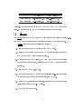
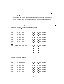
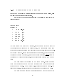
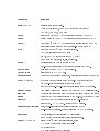
DLPROTEIN 1.2 User Manual
Contents
Overview
1
1 Building the molecular topology
3
1.1 dlgen : : : : : : : : : : : : : : : : : : :
1.1.1 dlgen input les : : : : : : : : : :
1.1.2 Editing the pdb le : : : : : : : :
1.1.3 Adding entries to the MBBT le
1.1.4 Adding entries to the PS le : : :
1.2 merge eld : : : : : : : : : : : : : : : :
2 The molecular dynamics code
2.1 Integration Algorithms : : : :
2.1.1 NVT ensemble : : : :
2.1.2 NPT ensemble : : : :
2.1.3 Constraints treatment
2.2 RESPA implementation : : :
2.3 Scanning neighbors : : : : : :
:
:
:
:
:
:
:
:
:
:
:
:
:
:
:
:
:
:
:
:
:
:
:
:
:
:
:
:
:
:
:
:
:
:
:
:
:
:
:
:
:
:
:
:
:
:
:
:
:
:
:
:
:
:
:
:
:
:
:
:
:
:
:
:
:
:
:
:
:
:
:
:
:
:
:
:
:
:
:
:
:
:
:
:
:
:
:
:
:
:
:
:
:
:
:
:
:
:
:
:
:
:
:
:
:
:
:
:
:
:
:
:
:
:
:
:
:
:
:
:
:
:
:
:
:
:
:
:
:
:
:
:
:
:
:
:
:
:
:
:
:
:
:
:
:
:
:
:
:
:
:
:
:
:
:
:
:
:
:
:
:
:
:
:
:
:
:
:
:
:
:
:
:
:
:
:
:
:
:
:
:
:
:
:
:
:
:
:
:
:
:
:
:
:
:
:
:
:
:
:
:
:
:
:
: 5
: 6
: 6
: 10
: 11
: 14
:
:
:
:
:
:
16
16
17
19
20
21
24
2.3.1 Memory optimization on scalar workstation
2.3.2 CPU optimization on scalar workstation : :
2.4 The Smooth Particle Mesh Ewald method : : : : :
2.4.1 Choosing the SPME variables : : : : : : : :
:
:
:
:
:
:
:
:
:
:
:
:
3 Other dierences between DLPOLY and DLPROTEIN
:
:
:
:
:
:
:
:
:
:
:
:
:
:
:
:
:
:
:
:
:
:
:
:
3.1 Non-bonded interactions : : : : : : : : : : : : : : : : : : : : : : : :
3.2 Interpolation, spline or direct evaluation of the Van der Waals interactions : : : : : : : : : : : : : : : : : : : : : : : : : : : : : : : :
3.3 Refolding of molecules : : : : : : : : : : : : : : : : : : : : : : : : :
3.4 Constraints treatment : : : : : : : : : : : : : : : : : : : : : : : : :
3.5 Shifted Van der Waals interactions and long range corrections : : :
3.6 Smoothing the Van der Waals interactions at the cut-o : : : : : :
3.7 Hydrogen bond detection : : : : : : : : : : : : : : : : : : : : : : : :
3.8 Short and long OUTPUT les : : : : : : : : : : : : : : : : : : : : :
3.9 I/O format of trajectory data : : : : : : : : : : : : : : : : : : : : :
3.10 Include les : : : : : : : : : : : : : : : : : : : : : : : : : : : : : : :
3.11 T3E communication routine : : : : : : : : : : : : : : : : : : : : : :
3.12 Directives in the CONTROL le : : : : : : : : : : : : : : : : : : : :
3.13 Directives in the FIELD le : : : : : : : : : : : : : : : : : : : : : :
3.14 Directives in the Makele : : : : : : : : : : : : : : : : : : : : : : :
3.15 Examples : : : : : : : : : : : : : : : : : : : : : : : : : : : : : : : :
References
24
25
26
27
29
29
29
30
30
31
31
32
32
32
33
33
34
36
37
39
41
i
Overview
DLPROTEIN is a molecular dynamics package written by Simone Melchionna
and Stefano Cozzini in the framework of the Italian Institute for the Physics of
Matter (INFM), Network on \MD simulation of biosystems". DLPROTEIN is a
development of the original general purpose Molecular Dynamics code DLPOLY
written at Daresbury Lab (UK) by William Smith and Tim R.Forester.
The motivation underlying the development of DLPROTEIN has been to
specialize the original MD code to deal more specically with biological molecules,
with particular focus on proteins, and with high eciency and low memory requirements for scalar architectures.
DLPROTEIN has been realized with the contributions of several people
who have partecipated in the project in dierent percentages. Amonst others we
wish to thank Antonella Luise as a coauthor of dlgen and for designing the link
cell algorithm for generic periodic boundary conditions, Maddalena Venturoli as a
coauthor of dlgen and for many useful insights in the code, Marco Pierro, as the
author of the merge eld utility, from the Physics Department of the University
\La Sapienza" of Rome. A special thanks is for Georges Destree, of the Universite
Libre de Bruxelles, who has managed several parallel xes and new algorithms in
the code.
During the development of DLPROTEIN collaboration and support from
Giovanni Ciccotti (University of Rome "La Sapienza"), Mattia Falconi, Alessandro
Desideri (University of Rome "Tor Vergata") and Mauro Ferrario (University of
1
Modena) are kindly ackowledged. We thank Tom Darden for providing us with
the SPME original routines.
The following manual is intended as an addendum to the DLPOLY 2.0
Manual [1]. The reader is referred to the DLPOLY manual for general explanations
about the code philosophy and technical details whereas the present documentation
reports only modications and addenda to the original DLPOLY package.
2
Chapter 1
Building the molecular topology
Building the molecular topology of molecules is done by the utility build all . The
program build all takes care of building up in sequence a system composed of
one or more molecules. build all is a fortran program that calls the two dierent
utilities called dlgen and merge eld .
The three programs build all , dlgen , and merge eld are provided with
a Makele in the build-topology directory. Once they are compiled (by simply
executing the \make" command), these utilities can be run alltogether, by running
the driver build all , or singularly.
dlgen converts a Protein Data Bank le (pdb le) into the les CONFIG
and FIELD that contain respectively the topology and conguration of a single
molecule. Subsequently merge eld merges each FIELD le produced by dlgen ,
eventually with other prebuilt FIELD les, into a global FIELD le. Theese utilities have been implemented thinking in terms of aminoacidic systems (e.g.proteins)
as the main goal, and it is able to treat force elds of the type CHARMm22 and
GROMOS87 (37c4 parameter set). Due to the general combination rules of
the CHARMm22 force eld, dlgen works for proteins, proteins+metallic groups
(e.g. heme group), phospholipids, sugars, and so on, i.e. any kind of entry can be
safely added to the molecular database. Viceversa due to the more complex rules
3
adopted by the GROMOS87 force eld (e.g. the way the dihedrals are dened for
sugars), the actual version of dlgen works only for proteins, eventually in presence
of metallic groups. The reader may ask the authors to obtain a non-standard
version of dlgen to treat dierent systems within the GROMOS87 force eld.
An easy way to run the build all utility is to make the following steps :
1. Link (or Copy) in your working directory the three executables produced by the compilation, together with the database les (MBBT and
PS les, as explained in the following) needed by dlgen to run. In the
working directory you need to have also the PDB les to be converted
or any previously produced FIELD le the needs to be merged.
2. Run the build all utility and answer a few questions. Infos and warnings
will be issued as the molecular construction proceeds.
The dlgen utility supports the \United Atom" (UA) scheme (i.e. CH, CH2
and CH3 group are treated as united groups) when using the GROMOS87 force
eld, and the \All Hydrogens" (AH) scheme (polar and non-polar hydrogens are
always explicitely treated) when using the CHARMm22 force eld.
dlgen uses an internal database to store the parameter set (PS) and the
molecular building block topology (MBBT), e.g. the structure of the elementary
units, such as the amino acids. The PS le stores:
- atomic names, masses and connection tables;
- bond reference list, spring constants and equilibrium distances;
- angle reference list, spring constants and equilibrium angles;
- dihedral reference list, multiplicity, force constants and phases;
- Van der Waals parameters.
The MBBT les stores the group names, internal connectivity and atomic
charges. In table 1.1 we report the database le names.
4
GROMOS87
CHARMM22
PS le name
MBBT le name
PS gromos37c.ff
MBBT gromos37c.ff
PS charmm22.ff
MBBT charmm22.ff
Table 1.1: Database le names for the GROMOS87 and CHARMM22 force
elds. PS : parameter set, MBBT : molecular bulding block topology
1.1 dlgen
The dlgen utility must be run with a pdb le that species a single molecule, i.e.
each atom of the molecule must be globally connected by chemical bonds.
dlgen performs in order the following actions :
1. Read in the Brookhaven pdb le and the MBBT les.
2. Generate the sequence of each block by merging the informations in
the pdb and MBBT les (edtgen routine).
3. If hydrogen atoms are missing, add them with the proper chemical
geometry and connectivity, as specied in the MBBT database (hgen
routine).
4. Read in the PS and FF.dat les.
5. Complete connectivity by adding the missing links (e.g. link aminoacid
to aminoacid, complete the aromatic rings, and so on).
6. Generate bond, angle and dihedral list, together with the Van der Waals
interactions (generic and I-IV types).
7. Dumps out the FIELD le.
5
1.1.1 dlgen input les
dlgen uses the following input data :
Brookhaven pdb le, containing atomic and molecular names and atomic
conguration. This le must be edited and modied, as explained later on.
FF.dat le, containing the topology title, constraints-vs.-harmonic springs
treatment and energy units. The constraints directives are :
directive:
constrain string
meaning:
where string can be equal to
all : all bonds are constrained
h : only bonds concerning hydrogens are constrained
none : all bonds are harmonic
specialbond n1 n2 n3 ::: list of residues to treat harmonically.
units string
Output units as expressed in the FIELD le. Admitted
values for string are \eV", \kJ", \kcal" and
\internal' for using dlpoly internal units.
Moreover the user must insert data as requested by the program in run time
at standard input.
1.1.2 Editing the pdb le
Before running the dlgen program the pdb le must be edited and a few changes
must be applied. dlgen uses each building block specied in the MBBT database
as an independent unit so that in principle there is no dierence when treating
a sequence of amino acids or a sequence of generic building blocks. In fact the
intrablock topology is specicied in the MBBT database, while dlgen uses the
geometry specied in the pdb le to construct the interblock topology.
1. Terminal groups labels
Usually the peptidic sequence begins (or ends) with a NH3 group. The
pdb atomic label relative to the starting nitrogen atom must be changed
from the original pdb label into the new NTER label and eventually if
6
any hydrogen is specied (i.e. the user does not require generation of
positions hydrogens from scratch) the hydrogen atoms must have the
labels HTn, with n=1, 2, 3. Hydrogen atoms attached to NTER must follow in order. In case the N-terminal aminoacid is a Proline, the name
of the starting nitrogen should be left as N and the aminoacid name
should be changed from PRO to PRT.
When the peptidic sequence has COO as a terminal group, the label
of the carbon atom must be changed into the CTER new label and the
oxygens must have the new labels OTn, with n=1, 2. Oxygens attached
to CTER must follow in order.
When having terminal PRO residues, the user must dene from scratch
the complete terminal residue (PRO+terminal group) in the MBBT le
as it is specied in the section about adding entries to the MBBT le.
2. Non aminoacidic specication
In the standard pdb format, non aminoacidic atoms have as special
molecular label HETATM instead of ATOM. The user must respect this
labeling when specifying groups as prosthetic groups, such as heme
molecule or single metals that are specied as separate entities in the
MBBT le.
3. Atom and block indexing
The pdb atomic indexing is ignored by dlgen . Viceversa the building
block (e.g. residue) indexing is used to signal the change in the molecular building block, althought the order of appearance is unimportant.
7
4. Protonation state and disulde bridges
Residues that in the pdb le have the same names but intrinsic dierences, e.g. dierent protonation states due to dierent pK's or disulde
brigdes, must be named consistently with the database names in the
MBBT le so that they adhere with the corresponding database denitions.
In the following example, it is indicated how to change the head and tail specication of a peptide. Given the original pdb le:
ATOM
1
N
ALA
1
15.850
25.550
23.340
ATOM
2
HT1 ALA
1
15.520
25.140
24.200
ATOM
3
HT2 ALA
1
15.700
26.540
23.360
ATOM
4
HT3 ALA
1
15.360
25.150
22.570
ATOM
5
CA
ALA
1
17.270
25.280
23.200
...
ATOM
1188
HZ3 LYH
128
31.830
21.930
16.050
ATOM
1189
C
LYH
128
27.000
27.260
13.390
ATOM
1190
OT1 LYH
128
26.420
28.360
13.350
ATOM
1191
OT2 LYH
128
26.460
26.250
12.940
...
You need to change it into :
ATOM
1
NTERALA%%
1
15.850
25.550
23.340
ATOM
2
HT1 ALA
1
15.520
25.140
24.200
ATOM
3
HT2 ALA
1
15.700
26.540
23.360
ATOM
4
HT3 ALA
1
15.360
25.150
22.570
ATOM
5
CA
1
17.270
25.280
23.200
ALA
8
...
ATOM
1188
HZ3 LYH
128
31.830
21.930
16.050
ATOM
1189
CTERLYH
128
27.000
27.260
13.390
ATOM
1190
OT1 LYH
128
26.420
28.360
13.350
ATOM
1191
OT2 LYH
128
26.460
26.250
12.940
...
9
1.1.3 Adding entries to the MBBT le
In the MBBT database the rst lines concern the gromos vs charmm signal, title
and number of subsequent block entries.
For each entry the format is specied as in the following example for the
alanine residue :
residue = ala
atoms = 6
1
N
N
-0.28
2
1H
H
.28
3
1CA
CH1
.0
4
3CB
CH3
.0
5
3C
C
.38
6
5O
O
- .38
The rst column (i4) is the atom indexing, second column (i4) is the index of
the preceeding atom linked to the current atom. The general rule is that each
attachment species only links with previously dened atoms. If the second column index is omitted, since it concerns interblock connectivity, or if the complete
connectivity cannot be specied, as is the case for aromatic rings, dlgen builds the
connectivity by using geometric rules, as coordinates are extracted from the pdb
le.
The third column (a4) regards the pdb atomic names, while the fourth
column (a4) species the atom type name (coherently with the atomic names as
specied in the PS le). The fth column (f8.0) species the atomic charge. The
last column (f8.0), if present, species the repetition of the current atom data.
The \nte" and \cte" block names as ctitious names and they need not to
10
be considered as new residue names, as they are needed only to specify data of the
terminal groups.
Some specic patched can be added to the MBBT le. These patches can be
necessary if dlgen fails to build the full topology of complex molecules. The patches
are used to add or delete specic constraints, angles bendings (harmonic type), dihedral torsions (cosine type), improper torsions (harmonic type) and bonds (harmonic types) potential terms from the nal topology. The general format of each
patch should be in the form :
add keyword num
list(1,...,n) par(1,m)
(in free format)
or
del keyword num
(in free format)
where keyword can be constraint, angle, dihedral, improper, bond. num is
the number of patches specied subsequently. list(1,...,n) is the list of atomic
indices involved in the patch indexed as the atoms appearance in the block itself.
par(1,...,m) is the list of parameters that need to be xed (appearing in the same
order of the FIELD le) in the same units as specied previously. An example
of patch can be found in the MBBT block specifying the HEME group (keyword
\hem").
list(1,...,n) par(1,m)
1.1.4 Adding entries to the PS le
The rst line of this le indicates the force eld type (charmm or gromos). Moreover, a line is skipped if starts with the character \#" while each new entry is
indicated by the special string BLOCK. The order of appearence of the BLOCKs
must be the same as the PS le included in the distribution. Atomic labels are
consistent with those specied in the fourth column of the MBBT le.
11
The database contains the following data:
Number of records in the atom list
Atom names (a4), masses (f12.0) and repetitions (i5)
Number of records in the bonds list
Prefactor for scaling the Van der Waals data between pairs
Bond pair names (2a4), force constants (f12.0) and equilibrium distances (f12.0)
Number of records in the angle bends list
Prefactor for scaling the Van der Waals data between atomic triplets
Angle triplet names (3a4), force constants (f12.0) and equilibrium angles (f12.0)
Number of records in the general proper dihedrals (GPD) list
Prefactor for scaling the Van der Waals data between atomic quadruplets of the GPD list
Potential type (cos), scaling factor for electrostatics and Van der Waals
interactions
GPD quadruplet names (4a4), force constants (f12.0), phase (f12.0)
and multeplicities (f12.0).
Number of records in the specic proper dihedrals (SPD) list
Prefactor for scaling the Van der Waals data between atomic quadruplets of the SPD list
12
Potential type (cos), scaling factor for electrostatics and Van der Waals
interactions
SPD quadruplet names (4a4), force constants (f12.0), phases (f12.0)
and multeplicities (f12.0).
Number of records in the general improper dihedrals (GID) list
Prefactor for scaling the Van der Waals data between atomic quadruplets of the GID list
Potential type (harm), scaling factor for electrostatics and Van der
Waals interactions
GID quadruplet names (4a4), force constants (f12.0), and equilibrium
angles (f12.0).
Number of records in the specic proper dihedrals (SID) list
Prefactor for scaling the Van der Waals data between atomic quadruplets of the SID list
Potential type (harm), scaling factor for electrostatics and Van der
Waals interactions
SID quadruplet names (4a4), force constants (f12.0), and equilibrium
angles (f12.0).
Number of records in the general Van der Waals parameters list
General Van der Waals parameters
Number of records in the specic Van der Waals parameters list
Specic Van der Waals parameters
13
Number of records in the general 1..4 Van der Waals parameters list
General 1..4 Van der Waals parameters
Number of records in the specic 1..4 Van der Waals parameters list
Specic 1..4 Van der Waals parameters
Here \general dihedrals" (both proper or improper) species the quadruplets having specied a reduced number of atoms dening the dihedral. The wild card
symbol \*" indicates all possible atom types included in the quadruplet. On the
other hand \specic dihedrals" means the quadruplets explicitily indicated.
Similarly \general" and \specic" Van der Waals interactions (for 1..4 interactions or not) refer to the parameter set used for all kind of atomic pairs and for
selected pairs respectively. The 1..4 parameters specify the interaction parameters
between pairs of atoms that are third neighbours in the molecular connectivity.
1.2 merge eld
This utility allows to merge dierent FIELD les into a single FIELD le, called
FIELD.out, where each starting FIELD le must contain one molecular specie.
Moreover each FIELD le must specify the Van der Waals parameters in \12-6"
style.
When running merge eld , the user is requested to provide as standard
input the force eld scheme (charmm or gromos), the name of each FIELD le,
together with the relative MBBT le and the number of repetitions of each molecular specie. If the name of some atom in one FIELD le coincides with the name
in a second FIELD les and those atoms have dierent interaction parameters, the
user is requested to change the name of atoms in the second FIELD le. This can
be done by the utility itself or by editing one of the FIELD les. The utility can
14
merge as many molecular species as needed by changing the mxmoltyps parameter in the merge eld.inc le and recompiling. The output les \VDW params"
and \SYSTEM" can be used by the user to check if the merging operation was
correctly achieved.
15
Chapter 2
The molecular dynamics code
2.1 Integration Algorithms
In DLPROTEIN the algorithm that integrates in time the equations of motion is
of the form of the Velocity Verlet (VV) scheme whereas in DLPOLY the original
scheme was the Leap Frog (LF) scheme. In addition the VV scheme is applied
in the form proposed in ref. [4] so to have, even in presence of non-hamiltonian
dynamics (as it is customary for generating canonical or isobaric ensembles), time
reversible and simplectic integrators.
Given the Hamiltonian equations of motion
r_ = mp
p_ = F
(2.1)
where velocities are related to momenta via the relation p = mv, the LF scheme
integrates the trajectory in time with the following updating scheme
r(t + h) = r(t) + hv(t + h=2)
v(t + h=2) = v(t ; h=2) + mh F (t)
(2.2)
together with the auxiliary equation to obtain velocities simultaneously to posi16
tions
v(t) = 12 [v(t ; h=2) + v(t + h=2)]
(2.3)
The VV scheme, that for hamiltonian system produces exactly the same trajectory
than the LF one, reads
2
r(t + h) = r(t) + hv(t) + 2hm F (t)
v(t + h) = v(t) + 2hm [F (t) + F (t + h)]
(2.4)
The VV scheme can be casted in operatorial form by using the Trotter
factorization of the evolution operator [4]
!
!
h
h
exp (ihLHam ) = exp i Lv exp (ihLr ) exp i Lv
2
2
!
!
!
hF
@
@
hF
@
= exp i 2m @v exp ihv @r exp i 2m @v
(2.5)
Each operator is applied sequentially and gives rise to a shift
@ )f (x) = f (x + a)
(2.6)
exp(a @x
In DLPROTEIN the single-time-step molecular dynamics is hadled by the routine
sloop, and the action of the propagators is performed by the routines
!
h
respa v verlet $ exp i 2 Lv
respa r verlet $ exp (ihLr )
applied according to the Trotter splitting. The same routines are called when
performing NVT and NPT simulations with slight modications for the NPT case
as explained in the following.
2.1.1 NVT ensemble
DLPROTEIN implements the canonical ensemble and the isobaric-isothermal ensemble with the Nose-Hoover style equations of motion[5]. Other kinds of statistical behaviours, such as the the Evans and Berendsen schemes can still be used.
17
The Nos-Hoover NVT equations of motion read
r_ = mp
p_ = F ; p
T
1
_ = 2 T ; 1
ext
T
(2.7)
Accordingly the integration scheme is given by the splitting
!
exp (ihL) = exp i h2 LNH exp (ihLHam ) exp i h2 LNH
where
!
@ + 1 T ; 1 @
iLNH = ;p @p
2 T
@
T
ext
(2.8)
(2.9)
For the NVT and NPT dynamics we make use of the general formula when applying
the eect of the thermostat and piston on the momenta and positions
"
#
exp (ax + b) @ = exp(a)x + b exp(a=2) sinh(a=2)
@x
(a=2)
(2.10)
The sinh(x)=x function is computed by expanding numerator and denominator to
a 8th order Taylor expansion.
The Nose-Hoover propagator is further symmetrically splitted in order to
deal with intrinsic momenta dependence of the thermostat driving force. The
splitting is of the type
"
#
T
@
h
h
1
exp(i LNH ) = exp 2
; 1 @
2
4
T
ext
T
# "
"
T
@#
@
h
1
h
exp ; 2 p @p exp 4 2 T ; 1 @
ext
T
(2.11)
The eect of the Nose-Hoover propagator is given by the routine
prop NH $ exp i h2 LNH
!
The same routine is applied for the NPT case with minor modications.
18
(2.12)
2.1.2 NPT ensemble
The NPT Nose-Hoover equations of motion are
r_ = mp + (r ; Ro )
p_ = F ; ( + )p
_ = 12 TT ; 1
ext
T
1
_ = 3Nk T 2 V (P ; Pext)
B ext P
V_ = 3V
(2.13)
where Ro is the total center of mass of the system. The Trotter splitting is chosen
as
!
!
h
h
0
0
0
exp (ihL) = exp i 2 LNH exp (ihLHam ) exp i 2 LNH
(2.14)
where
@ + 3V @
iL0Ham = iLHam + (r ; Ro ) @r
@V
@
iL0NH = ;( + )p @p
T
@
@
1
+ 2 T ; 1 @ + 3Nk 1T 2 V (P ; Pext) @
T
ext
B ext P
(2.15)
The NPT Nose-Hoover propagator is further symmetrically splitted in order to
deal with intrinsic momenta and coordinates dependence of the thermostat and
piston driving forces. The splitting is analogous to equation 2.11. The eect of
the NPT Nose-Hoover propagator is again given by the routine
!
h
prop NH $ exp i 2 L0NH
(2.16)
The NST ensemble equations of motion, i.e. the dynamics associated with
anisotropic volume uctuations, are not yet implemented in the current release.
For the Berendsen thermostat, the evolution propagator has been splitted
in an analogous way to the Nose-Hoover way. The routine that scales the velocities
according to the Berendsen scaling factor is prop ber.
19
The Evans constraint on velocities, that allows to sample the isokinetic
ensemble, is achieved in the routine evans scale.
2.1.3 Constraints treatment
In the VV scheme treatment of the holonomic constraints is handled in a similar
way to the LF scheme. The main dierence relies in imposing simultaneously the
condition of satised constraints
k (frig) = 0
k = 1; M
(2.17)
as handled by the routines rdshake 1 and sca shake (SHAKE procedure) and
condition that momenta are orthogonal to the constraints surfaces
_ k (fri; pig) = 0
(2.18)
as handled by the routines quench and quench1 (known as the RATTLE procedure). We have modied the preexisting rdshake 1 routine into the new sca shake
routine. The change has been made in order to solve the iterative sequence of constraints by cyclic update of atomic positions [3]. At the moment this procedure is
possible only on scalar architectures. Viceversa the previous rdshake 1 is applied
on the full sequence of constraints in a dierent way and it has been motivated by
parallelisation reason [1]. The sca shake, althought running on scalar platforms,
converges in about half the iterations than the parallel version. In an analogous
way the new sca quench routines uses a cyclic update of atomic velocities.
For the NVE and NVT ensembles the sequence of propagators and constraints impositions is
!
!
!
!
h
h
h
h
exp i LNH R exp i Lv S exp (ihLr ) exp i Lv exp i LNH
(2.19)
2
2
2
2
where R and S are the operators that handle constraints on velocities and positions
respectively.
20
In the NPT implementation the overall procedure is modied in order to
deal with intrinsic dependence of the pressure tensor on the constraining forces,
as discussed in [4]. In this case an iteration loop need to be applied in order to
converge the pressure estimate and piston update so to achieve proper integration
in time. Convergence of the piston updating is controlled by the routine checkexp.
For the Berendsen isothermal + isobaric dynamics, the splitting of the propagator is rather crude, but it seems to produce a statistical behaviour rather similar
to the Berendsen implementation of the original DLPOLY package.
2.2 RESPA implementation
A multiple time step implementation, generally known as the RESPA method, has
been applied in the framework of the VV scheme [4] and within a splitting of the
Hamiltonian well suited for biological systems [6]. The propagator is in the form
exp(ihL) = exp[ih(Lo + L1 + L2 + L3 )]
(2.20)
where Lo takes into account positions shifts and updating of momenta according
to bond stretching and angle bending forces. L1 shifts momenta due to dihedral
torsions and rst-shell non-bonding interactions. L2 shifts momenta due to secondshell non-bonding interactions and reciprocal Ewald term. L3 shifts momenta due
to third-shell non-bonding interactions [6]. First, second and third non-bonding
forces are dened by introducing three interaction ranges
0 < rij < rcut1
rcut1 < rij < rcut2
rcut2 < rij < cuto
(2.21)
where for Van der Waals interaction cuto is substituted by the variable rvdw
in the CONTROL le. The shells are handled via proper switching functions in
21
order to ensure continuity of forces at the shell borders. The switching functions
are polynomials of order three governed by the \healing length" parameter switch.
The splitted propagator is of the form
[exp(i h23 L3 )[exp(i h22 L2)[exp(i h21 L1 )
[exp(ihLo )]no
exp(i h21 L1 )]n1 exp(i h22 L2)]n2 exp(i h23 L3 )]
(2.22)
where h is the input time step and no, n1 and n2 are chosen in order to have the
following time steps of increasing lengths
h1 = n0 h
h2 = n1 h1 = n1n0 h
h3 = n2 h2 = n2n1 h1 = n2n1 n0 h
(2.23)
When using this splitting within the VV scheme and with the previously reported
NVT and NPT dynamics, changes need to be applied with respect to the previous
LF scheme. The reader is referred to the cited literature for a detailed explanation
of technical points.
Switching between single and multiple time step molecular dynamics is
achieved by changing the input parameters in the CONTROL le (see the mult
directive in the CONTROL le). For example setting
rcut1 0:0
rcut2 0:0
cuto 10:0
rvdw 10:0
mult 1 1 1
22
(2.24)
is a typical setting for a single time step simulation whilst
rcut1 7:0
rcut2 9:0
cuto 10:0
rvdw 10:0
mult 2 3 2
(2.25)
is a possible choice for a multiple time step simulations. The multiple-time-step
algorithm is handled by the routine mloop.
23
2.3 Scanning neighbors
DLPROTEIN retains the previous capabilities of DLPOLY to scan neighbors on a
\all-pairs" (AP) basis by using a Brode-Alrich algorithm to order the interacting
pairs and eventually split them on several processors.
A direct scanning method based on the Link Cell (LC) method [2] is also
been preserved, but DLPOLY supported only cubic or orthorombic PBC for the
LC method. The LC method allows a drastic raise in CPU eciency for large
systems since CPU time grows linearly with the system size (AP is quadratic).
Those scanning methods have been modied in order to
implement AP and LC on scalar platforms and optimize CPU and
memory use.
extend LC to dierent PBC's (truncated octahedron and dodecahedron.
Actually in the CONTROL le it is possible to chose whether to use AP or LC
method. The LC method is applied with dierent methods if the run is scalar or
parallel. In the case of a parallel run LC is activated only if it produces eective
CPU optimization and this condition is true if
cuto min(Lx; Ly; Lz)=3
(2.26)
With a scalar run the condition is less strict. If LC is not usable, eventually due
to a cell shrinking as time proceeds with an isobaric run, automatic switching to
AP scanning is performed and the user is informed.
2.3.1 Memory optimization on scalar workstation
DLPROTEIN has routines that optimize memory handling by substituting a 2darray array for storing interacting pairs into a 1d-array. The method is suited
24
to run on scalar machines and a good speed-up is achieved with respect to other
methods due to a better cache memory use.
An extra factor 2 in memory is gained by using the \INTEGER*2" denition
for the interacting list. This is actually suited for number of atoms less than
32767, if this is not the case an error message is printed out and the code must be
recompiled.
2.3.2 CPU optimization on scalar workstation
The actual version of DLPROTEIN handles the Link Cell method [2] for all possible boundary conditions implemented in the code. A dierent algorithm than
in the original DLPOLY routine has been implemented. The routines that perform
LC scanning on scalar workstation are scalink vlst cube and scalink respa vlst cube
for cubic and octahedral boxes, scalink vlst ortho and scalink respa vlst ortho
for general triclinic boxes.
25
2.4 The Smooth Particle Mesh Ewald method
DLPOLY used the Ewald method to compute the electrostatic interactions when
using periodic boundary conditions [1]. The Ewald method splits the Coulombic
interactions into two separate potentials in the form
(
)
N q q
M
X
X X
1
erc(rlm)
1
j n
erfc
(
r
q
Uc = 4
nj ) ;
l qm lm p +
1;lm
4o molecules lm
rlm
o n<j rnj
+ Urec
(2.27)
where Urec is the reciprocal space term of the Ewald sum
1 exp(;k2 =42 ) X
N
X
Urec = 2V1 j
qj exp(;ik rj )j2
k2
o o k6=0
j
(2.28)
as implemented in the ewald1 routine of the original DLPOLY code and it is
usually the main CPU-eater in biosimulations, moreover scaling as N 3=2 with the
system size.
Alternatively DLPROTEIN can use the smooth particle mesh Ewald (SPME)
method [7] to compute the reciprocal part of the Ewald sum. The SPME method
does not compute Urec as a sum over k-shells as for the original Ewald method,
but it uses a three-dimensional grid to apply 3d-Fast Fourier Transforms (FFT)
and obtain splined observables that reconstruct the requested energy term and
corresponding forces. The SPME is called by the routine ewald1pme, a driver
for the original SPME routines.
The SPME method requires as input parameters the order of the spline
and the number of grid points in the x-, y- and z-directions. These parameters
are specied in the CONTROL le as described in the following sections. Memory
requirements must be satised by changing the MAXN, MAXORDER and MAXT
parameters in the ewald1pme routine. If memory is necessary, i.e. for very dense
grids or high order splines, the program will write the memory requirements and
the code must be recompiled.
26
The SPME method is currently available only for general triclinic boxes so
that it is forbidden for truncated octahedral and rhombic dodecahedral boxes.
SPME uses a public domain FFT routine or, alternatively, calls to libraries
optimized on selected architectures (as Silicon Graphics and Cray machines, while
the user can extend the calls to other platforms) The use of public domain or
library calls to apply FFT is chosen in the compilation environment, as discussed
in the section on the compilation directives. The parallel implementation of SPME
is achieved by using the distributed routine \pcct3d" to perform 3d-FFT, present
on T3E and Silicon Graphics parallel architectures.
2.4.1 Choosing the SPME variables
The precedure for choosing the SPME control variables resembles the procedure
usually applied in the standard Ewald sum method (e.g. see the DLPOLY manual). The only dierence relies in substituing the number of k-vectors of the standard Ewald sum with the number of grid points of the SPME real space method.
Furthermore in the SPME another factor can be varied so to achieve optimal convergence, this is the order of the splines used in the method. It is advised to use
a well established and safe value of the spline order, say 6 or 8, and to focus on
a good choice of the SPME variables, since the spline order does not aect the
results if the spline order is large enough.
In the original Ewald method the "ewald precision" directive was available
to nd an optimal value of and kmax . The same directive can be used in order to
nd a good guess for , but still a choice for the grid density must be taken. So,
it is recommended to determine the and n parameters manually, as described in
the following (and as almost identically described in the DLPOLY manual).
Preselect the value for rcut, choose a value for of about 3:2=rcut and a
large value for n (say 50 50 50 or more). Then do a series of ten or so single
27
step simulations with your initial conguration and with ranging over the value
chosen plus and minus 20%. Plot the Coulombic energy (and the coulombic virial
with opposite sign, ;W ) versus . If the SPME is correctly converged you will
see a plateau in the plot. Divergence from the plateau at small is due to nonconvergence in the real space sum. Divergence from the plateau at large is due to
non-convergence of the SPME term. Redo the series of calculations using smaller
n values and by choosing the n parameters such that they can be only divided by
2, 3 or 5 (e.g. 50, 48, 45, ...). The optimum values for n are the smallest values
that reproduce at the value of to be used in the simulation the correct Coulombic
energy (the plateau value) and virial. Keep in mind that the virial depends on
forces and it converges more slowly than the energy - i.e. one usually requires a
higher precision in the energy, say 10;6, than in the virial.
28
Chapter 3
Other dierences between
DLPOLY and DLPROTEIN
3.1 Non-bonded interactions
In DLPROTEIN the actual number of available non-bonding potentials has been
restricted in order to deal only with potentials usually employed in biological simulations (e.g. the GROMOS and CHARMM22 force elds). This is the Coulomb
interaction (in the form bare 1=r form, shifted, reaction eld or Ewald sum) and
the Van der Waals interaction, both in the 12-6 and lj form for the input FIELD
le.
3.2 Interpolation, spline or direct evaluation of
the Van der Waals interactions
In order to increase performances DLPROTEIN can avoid the use of tabulated
potential when computing the non-bonding forces. On the other hand splines can
be used as a third alternative. Higher order interpolation schemes, such as the 4points and r-square interpolation, as used in the original DLPOLY program, have
29
been eliminated. Interpolation (or spline) versus direct evaluation is managed in
the CONTROL le. The directive \interpolate potentials" is used to indicate the
use of an interpolation or a splining scheme. At the compilation level, when the
compilation macro \SPLINE" is present the splined potential will be used instead
of the 3-point interpolation. In the include le, specication of the grid points for
the spline is determined by the parameter mxspln. The ratio between the grid
points in a 3-point interpolation and spline potential can be up to 10 depending
on the desired accuracy.
3.3 Refolding of molecules
An ecient way of reducing CPU time when dealing with molecules is to avoid
molecule refolding in the primary cell of periodic boundary condition setting. Refolding means that molecules will be cut appear as cut in the primary cell. By
avoiding refolding routines dealing with constraints will strongly ameliorate in performance. Refolding of molecules (as used originally in DLPOLY) is activated at
the compilation level by the macro REFOLD, while by default the code will run
without any refolding.
If refolding is absent the code will sew the molecules at step zero of the MD
run in the routine utaylor. When a molecular species is constituted by blocks not
connected by constraints or springs, refolding of molecules is mandatory.
3.4 Constraints treatment
In order to have exactly the same trajectories on scalar and parallel platforms, i.e.
avoiding the dierent ways the shake algorithms is implemented in the sca shake
and rdshake 1 routines, it is possible to force the code to use sca shake also with
parallel runs, where all processors will process all the constraints in the system.
30
This is achieved by specing the macro SERIALSHAKE at the compilation level.
3.5 Shifted Van der Waals interactions and long
range corrections
Better energy conservation is achieved when the Van der Waals potential is shifted
at the chosen cut-o. The shift is activated through the ljshift potential directive
in the CONTROL le.
The shift does not aect the forces but only the energy. Consequently the
NVE trajectory of a shifted and unshifted potential will be exactly the same apart
from a uctuating term in the total energy. Consistently with the shifted potential
model, the long range corrections to energy and pressure are set to zero. In this
case the dynamics of the system is aected when performing NPT dynamics since
in the unshifted system the long range correction to pressure is part of the pressure
tensor and its act as a pseudo-force for the volume rearrangement.
3.6 Smoothing the Van der Waals interactions
at the cut-o
A switching function can be used in order to eliminate discontinuities in the forces
at the cut-o for the Van der Waals potential. Switching is obtained by a 3rd order polinomial function that switches o the potential energy in the range
(rcut ; dswch) < r < rcut, where dswch is the healing length as specied in the
CONTROL le by the directive ljswitch.
31
3.7 Hydrogen bond detection
In DLPROTEIN it is possible to analyse the presence of hydrogen bonds in the
system during the run. The detection of hydrogen bonds is stored in the output
le HBOND.dat in formatted (20i5) style, as the list of atomic indices of triplets
of donor-hydrogen-acceptor.
Hbond formation is controlled by the directive hbond n dist angle in the
CONTROL le, where n is the frequency for dumping the detected Hbonds, dist
is the distance between donor and acceptor and angle is the angle formed between
the vector connecting hydrogen-donor and the vector connecting acceptor to donor.
The specication of donors, polar hydrogens and acceptors in the system is
specied in the FIELD le, as explained in the following.
3.8 Short and long OUTPUT les
When running biological molecules, i.e. when using very large FIELD les, the
user may require that the OUTPUT le is shorter than the default value. A short
or long version of the OUTPUT le can be obtained by using the directives output
short and output long in the CONTROL le.
3.9 I/O format of trajectory data
A compact and formatted version of the dumped output trajectory is often useful
with biomolecules. A formatted GROMOS-like version of the output data can
be generated by using the directive gromos dump in the CONTROL le. In
this case three dierent les, DUMPPOS.dat, DUMPVEL.dat, DUMPFOR.dat,
are used to dump positions, velocities and forces separately. This is the default
behaviour. When using the history dump directive the old style HISTORY le
is recovered.
32
3.10 Include les
The main include le of DLPROTEIN is dlprotein.inc that should be modied
for any change, in an analogous way to the dl params.inc le for DLPOLY. In
the utility directory the code parset dlprotein.f has been added, analogous to
the parset utility for DLPOLY.
A new include les has been added in DLPROTEIN that is used for declaring the arrays dimensions used in the SPME method. This le is called darden.inc
(where its analogous for the T3E compilation is darden t3e.inc).
3.11 T3E communication routine
A new version of the routines gdsum and gisum have been introduced to strongly
reduce communication times on the Cray T3E parallel architecture.
33
3.12 Directives in the CONTROL le
In table 3.1 we report the directives in the CONTROL le that are changed or are
not standard in the original DLPOLY2.0 package.
None of the added directives is mandatory. If not specied rcut1, rcut2,
rvdw and the switching length are set to zero and the single time step scheme is
applied.
34
directive:
mult n0 n1 n2
meaning:
multiple time steps cycles.
Given the timestep h, the RESPA timesteps are given by
h1 = n0 h, h2 = n1 h1 , h3 = n2 h2
rcut1 f
First cuto (
A) for C+VdW interaction (region I of RESPA)
rcut2 f
Second cuto (
A) for C+VdW interaction (region II of RESPA)
cuto f
Last cuto (
A) for C+VdW interactions (region III of RESPA or
global interaction region with the single-time step scheme)
rvdw f
Maximum cuto (
A) for VdW interactions.
VdW are globally computed within
the (0; rvdw + swlen) sphere if rvdw < cutoff
and within the regions I, II, III, otherwise.
switch f
Healing length (
A) for switching o the
non-bonding interactions at the region borders for RESPA.
output long
Verbose mode in OUTPUT le (default).
output short
Silent mode in OUTPUT le.
gromos dump
Three dumping les for trajectory, velocities and forces (Gromos sty
hbond n dist ang
Hydrogen bond detection every n steps. Hbond is detected if
the donor-acceptor distance is less than dist (
A)
and the hydrogen-donor-acceptor angle is less than ang degrees.
history dump
One history le for dumping the MD run (DLPOLY original style).
link cell
Activates the link cell method whenever the ratio between the cell d
ljshift
Shift the Van der Waals potential at the cut-o. Not shifted by defa
ljswitch f
Smoothed Van der Waals potential at the cut-o in the
region rcut ; f < r < rcut. Unsmoothed by default.
interpolate potentials Uses the r-interpolated or splined evaluation of the
non-bonding potentials. Direct evaluation of VdW by default.
maxwell n
Global refresh of velocities from a Maxwellian
every n steps (preferentially during equilibration).
spme n nx ny nz
select SPME35method for elecrostatics, with:
= Ewald convergence parameter (
A;1)
n = spline order
sitnam
weight
chge
nrept
ifrz
igrp
hprop
a8
f12.0
f12.0
i5
i5
i5
a3
atomic site name (unchanged)
atomic site mass (unchanged)
atomic site charge (unchanged)
repeat counter (unchanged)
'frozen' atom (unchanged)
neutral/charge group number (unchanged)
Hbond propensity (added)
Table 3.2: Atomic sites specication in the FIELD le
3.13 Directives in the FIELD le
The only optional change in the FIELD le for DLPROTEIN is the specication
of the donors, polar hydrogens and acceptors to detect Hbond formation in runtime. The format of the FIELD le regards the atomic species description, and
appears as (a8,2f12.0,3i5,a3) (see table 3.13) The keyword hprop is equal to
\d.." for a donor, \.h." for a polar hydrogen attached to a donor, \..a" for an
acceptor, \d.a" for an atom with both acceptor and donor propensity.
The mandatory rule to use when specifying polar hydrogens is that all
polar hydrogens attached to a donor must follow in order the donor specication.
Absence of a proper triplet will be set to \..." by default.
36
3.14 Directives in the Makele
In this section fwe describe the Makele directives added or changed with respect
to the original DLPOLY2.0 package.
1. VECTLIST
This macro compiles the code to run with a 1-d array for storing the
neighbors table. It is usable only with scalar architectures. It allows
an optimal save in memory and CPU time. The arguments are:
VECTLIST - 1-d array (default)
NOVECTLIST - 2-d array
2. STORE
This macro compiles the code to run with a 2 bytes declaration of
neighbor arrays. It allows a factor 2 in savins memory. Allowed only
for number of atoms less then 32767. The arguments are:
STORE2 - INTEGER*2 declaration(default)
STORE4 - INTEGER*4 declaration
3. FFT
This macro uses a public domain or library versions of the Fast Fourier
Transforms to apply the SPME method. The arguments are:
PUBFFT - for serial public domain FFT (default)
SGIFFT - for serial Silicon Graphics complib library
CRAYFFT - for serial Cray libraries
PCCFFT - for parallel library with the pcct3d distributed routine
available.
4. SHAKE
This macro forces the use of the standard shake algorithm to treat
37
constraints on parallel architectures (constraints are not distributed
and all processors perform the same task). The argument are :
SERIALSHAKE - to force serial shake with parallel runs
NOSERIALSHAKE - to use distributed shake algorithm (default).
5. INTERPOLATE
Switch of the calculation of potentials and forces between 3-point interpolation and cubic spline. Arguments :
SPLINE - Spline potential
NOSPLINE - 3-point interpolation (default).
6. REFOLD
Controls molecules refolding in the primary box when using periodic
boundary conditions. Arguments :
REFOLD - Molecules are refolded, i.e. broken, in the primary cell
NOREFOLD - Molecules are not refolded (default).
38
3.15 Examples
A few examples are provided together with DLPROTEIN. The examples are kept
in the \examples" directory and they are :
1. System composed of 500 argon atoms simulated for 1000 steps.
Ensemble : NVE
Van der Waals interaction : shifted + smoothed. Direct evaluation
No electrostatics
Scanning : all pairs basis
2. System composed of 256 SPC water molecules, 100 steps.
Ensemble : NVT (Nose-Hoover)
Van der Waals interaction : shifted + smoothed. Splined potential
Electrostatics : SPME
Scanning : all pairs basis
3. System composed of 256 SPC water molecules, 200 steps.
Ensemble : NPT (Nose-Hoover)
Van der Waals interaction : shifted + smoothed. Direct evaluation
Electrostatics : Ewald sum
Scanning : all pairs basis
4. System composed of Myoglobin + 1513 tip3p water molecules + 9 Cl
counterions, 20 steps.
Ensemble : NPT (Nose-Hoover)
Van der Waals interaction : shifted + smoothed. Direct evaluation
Electrostatics : SPME
Scanning : link cell method
39
In the \build-topology" directory an example of use of the build all utility
is provided. The example builds the topology of Myoglobin as used in the previous
test case. The utility build all can be run by answering a few questions or by using
the prebuilt le with the command
build all < input build all > out build all
A number of les are produced as execution proceeds. The output le FIELD.out
is the global topology of Myoblogin + solvent + counterions. The topology of
tip3p water and counterions are present as prebuilt FIELD les. The output les
FIELD.1 and CONFIG.1 are the partial topology and conguration for Myoglobin.
The CONFIG.1 le can be used in conjunction with the DLPOLY utility wateradd to ll the MD box with water.
40
Bibliography
[1] Smith, W., Forester, T.R. , \The DlPoly 2.0 User Manual", T.R.Forester
and W.Smith, CCLRC, Daresbury Laboratory, Daresbury, Warrington
WA4 4AD, England (1995).
[2] M.P.Allen e D.J.Tildesley, \Computer simulation of liquids", Clarendon
Press, Oxford, 1987.
[3] Ciccotti, G., and Ryckaert, J.P., Comp.Phys.Rep.4(1986), 345
[4] Martyna, J.G., Tuckerman, M.E., Tobias, D.J., Klein, M.L.,
Mol.Phys.87(1996), 1117
[5] Melchionna, S., Ciccotti, G., Holian, B.L., Mol.Phys.78(1993), 533
[6] Procacci, P., Marchi, M., J.Chem.Phys.104(1996), 3003
[7] Essmann, U., Perera, L., Berkowitz, M.L., Darden, T., Lee, H., Pedersen, L.G. J.Chem.Phys.103(1995), 8577
41