Download User Manual: Product Name

Oracle Financial Services Operational Risk
Economic Capital
User Guide
Release 2.1
April 2012
User Guide: Oracle Financial Services Operational Risk Economic Capital, Release 2.1
What’s New in this Release
This section identifies updates in the Oracle Financial Services Operational Risk Economic
Capital, Release 2.1.
Oracle Financial Services Operational Risk Economic Capital Release 2.1 now supports additional
10 truncated distributions for modeling the severity of internal loss data and duly scaled external
loss data. The additional distributions are as follows:

Truncated Burr

Truncated Exponential

Truncated Gamma

Truncated Gumbel

Truncated Log-Gamma

Truncated Log-Logistic

Truncated Log-Normal

Truncated Pareto

Truncated Uniform

Truncated Weibull
Oracle Financial Services Software Confidential-Restricted
ii
User Guide: Oracle Financial Services Operational Risk Economic Capital, Release 2.1
Contents
WHAT’S NEW IN THIS RELEASE ................................................................................................... II
ABOUT THE GUIDE ........................................................................................................................ VI
SCOPE OF THE GUIDE ..................................................................................................................................................... VI
AUDIENCE ................................................................................................................................................................... VI
WHERE TO FIND INFORMATION ....................................................................................................................................... VI
HOW TO USE THIS USER GUIDE....................................................................................................................................... VII
COMMON ICONS ......................................................................................................................................................... VII
DOCUMENT CONVENTIONS ........................................................................................................................................... VIII
1.
INTRODUCTION ....................................................................................................................... 1
1.1.
2.
OVERVIEW OF THE APPLICATION .........................................................................................................................1
UNDERSTANDING THE APPLICATION ............................................................................... 3
2.1.
PRE MODEL....................................................................................................................................................3
2.1.1. Standard Reporting Group .....................................................................................................................4
2.2.
MODELING ATTRIBUTES ....................................................................................................................................5
2.2.1. Rule Framework: Loss Data and Loss Threshold Capture ......................................................................6
2.2.2. Rule Framework: Reclassification ..........................................................................................................7
2.2.3. Model Execution ....................................................................................................................................8
2.2.4. Stress Testing .......................................................................................................................................13
2.3.
OPERATIONAL RISK ECONOMIC CAPITAL - FUNCTIONAL PROCESS FLOW DIAGRAM .....................................................14
2.4.
OPERATIONAL RISK ECONOMIC CAPITAL – PRODUCT PROCESS FLOW ......................................................................14
2.4.1. Tab.1: Capital Calculation ....................................................................................................................15
2.4.2. Tab.2: Loss Data Frequency .................................................................................................................18
2.4.3. Tab.3: Loss Data Severity .....................................................................................................................19
2.4.4. Tab.4: Scenario Data ............................................................................................................................20
2.4.5. Tab.5: Credibility Factor .......................................................................................................................21
2.4.6. Tab.6: Data Transformation ................................................................................................................22
2.4.7. Tab.7: Filter ..........................................................................................................................................23
2.5.
STRESS TESTING OVERVIEW .............................................................................................................................23
3.
PREPARING FOR EXECUTION............................................................................................. 28
3.1.
3.2.
SET UP DEFINITION .........................................................................................................................................28
STAGING AREA ..............................................................................................................................................30
4.
EXECUTION ..............................................................................................................................31
5.
OPERATIONAL RISK ECONOMIC CAPITAL REPORTING .............................................. 32
FREQUENTLY ASKED QUESTIONS ............................................................................................. 34
ANNEXURE A: THINGS TO REMEMBER.................................................................................... 37
ANNEXURE B: UNDERSTANDING KEY TERMS AND CONCEPTS ....................................... 38
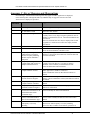
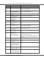
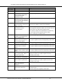
ANNEXURE C: ERROR MESSAGES AND OBSERVATIONS .......................................................41
ACRONYMS AND GLOSSARY TERMS ........................................................................................... 45
INDEX ................................................................................................................................................ 46
Oracle Financial Services Software Confidential-Restricted
iii
User Guide: Oracle Financial Services Operational Risk Economic Capital, Release 2.1
List of Figures
Figure 1: Functional Flow of Operational Risk Economic Capital Application .................................................... 14
Figure 2: OREC modeling............................................................................................................................................... 15
Figure 3: Operational Risk Economic Capital Model Definition Screen ................................................................ 16
Figure 4: Reporting Group Relevance Setting Screen ................................................................................................ 16
Figure 5: Parameters ......................................................................................................................................................... 17
Figure 6: Simulation Settings and Options Screen ...................................................................................................... 17
Figure 7: Frequency Distribution Selection .................................................................................................................. 18
Figure 8: Severity Distribution Selection....................................................................................................................... 20
Figure 9: Scenario Analysis Screen ................................................................................................................................. 20
Figure 10: Credibility Factor ........................................................................................................................................... 22
Figure 11: Data Transformation ..................................................................................................................................... 23
Figure 12: Filters ............................................................................................................................................................... 23
Figure 13: Variable Definition Selection ....................................................................................................................... 24
Figure 14: Variable Management Screen ....................................................................................................................... 24
Figure 15: Variable Definition Screen ........................................................................................................................... 25
Figure 16: Variable Shock Definition ............................................................................................................................ 25
Figure 17: Scenario Definition ........................................................................................................................................ 26
Figure 18: Stress Definition Screen ................................................................................................................................ 26
Figure 19: Sandbox Definition........................................................................................................................................ 28
Figure 20: Operational Risk Economic Capital Modeling: Business Model Browser ........................................... 29
Figure 21: Model Deployment Screen – 1 .................................................................................................................... 30
Figure 22: Model Deployment Screen – 2 .................................................................................................................... 30
Figure 23: Expected and Unexpected Loss .................................................................................................................. 38
Figure 24: Data Warehouse Schemas ............................................................................................................................ 39
Oracle Financial Services Software Confidential-Restricted
iv
User Guide: Oracle Financial Services Operational Risk Economic Capital, Release 2.1
List of Tables
Table 1: Common Icons ................................................................................................................................................. viii
Table 2: Document Conventions .................................................................................................................................. viii
Table 3: Standard Reporting Group ................................................................................................................................ 4
Table 4: Reclassification Example .................................................................................................................................... 4
Table 5: Scaling in Rule Framework ................................................................................................................................ 7
Table 6: Deductible Model .............................................................................................................................................. 12
Table 7: Proportionate Model with Single Offset ....................................................................................................... 12
Table 8: Credibility Factor ............................................................................................................................................... 22
Table 9: Error Messages .................................................................................................................................................. 43
Table 10: Peculiar Observations ..................................................................................................................................... 44
Oracle Financial Services Software Confidential-Restricted
v
User Guide: Oracle Financial Services Operational Risk Economic Capital, Release 2.1
About the Guide
This section provides a brief description of the scope, the audience, the references, the
organization of the User Guide, the common icons in the application and conventions incorporated
into the User Guide. The topics in this section are organized as follows:

Scope of the Guide

Audience

Where to Find Information

How to Use this User Guide

Common Icons

Document Conventions
Scope of the Guide
The objective of this User Guide is to provide a comprehensive working knowledge to the users
on Oracle Financial Services Operational Risk Economic Capital, Release 2.1. This User Guide is
intended to help the user understand the key features and functions of Operational Risk Economic
Capital application and use the application effectively. However, this User Guide is not meant to
provide guidance on how to install and use Oracle Financial Services Analytical Application
Infrastructure (OFSAAI). This User Guide is also not meant to provide details on installation of
Oracle Financial Services Operational Risk Economic Capital, Release 2.1 data model.
Audience
This manual is intended for the following audience:

Technical Analyst: This user ensures that the data is populated in the relevant tables as per
the specifications. The user executes, schedules, and monitors the execution of Runs as
batches.

Business User: This user reviews the functional requirements and information sources,
like reports.

Data Analyst: This user cleans, validates and imports data into the OFSAAI Download
Specification format.

Administrator: The Administrator maintains user accounts and roles, archives data, loads
data feeds, and so on. The administrator controls the access rights of users.
Where to Find Information
For additional information on Oracle Financial Services Operational Risk Economic Capital,
Release 2.1, refer to the following documents:

Business Metadata Documents: These documents are grouped into two sets as follows:

Oracle Financial Services Operational Risk Economic Capital Release 2.1
Business Metadata.xls: This document contains the definitions of the
Business Metadata like Measures, Business Processors, Hierarchies,
Hierarchy Attributes, Aliases, Derived Entities and Datasets present in
OREC Application.

Oracle Financial Services Operational Risk Economic Capital Release 2.1
Rule Metadata.xls: This document contains the definitions of Rules,
Pooling, Optimizer and Processes.
Oracle Financial Services Software Confidential-Restricted
vi
User Guide: Oracle Financial Services Operational Risk Economic Capital, Release 2.1

Technical Metadata: This document contains the definitions of the Table to Table (T2T)
used in various portions of OREC application.

Download Specifications: The format and structure of the RDBMS tables is specified in
the Download Specifications (DL Specs). Download Specifications contain details of the
attributes required for processing in OREC Application.

OFSAAI documents: The set of OFSAAI documents packaged in the installer will help
the user understand the functions of the various components of Oracle Financial Services
Analytical Application Infrastructure (OFSAAI) used for OREC computation.

Application Installation Manual
How to use this User Guide
The information in this User Guide is divided into the following chapters

Chapter 1: “Introduction”: The objective of this chapter is to introduce the user to Oracle
Financial Services Operational Risk Economic Capital, Release 2.1 and provide an
overview of OREC Application.

Chapter 2: “Understanding the Application”: The objective of this chapter is to provide an
understanding to the user on the various functions of OREC application.

Chapter 3: “Preparing for Execution”: The objective of this chapter is to provide a detailed
explanation of the activities involved before actual execution of Runs such as data
maintenance and so on.

Chapter 4: “Execution”: The objective of this chapter is to inform the user on the
execution function of OREC application.

Chapter 5: “Operational Risk Economic Capital Reporting”: The main objective of this
chapter is to provide a brief description of the reporting functionality in OREC
Application.
Common Icons
The common icons incorporated into OREC application are as follows:
Icons
Description
Use this icon to add a new entry.
Use this icon to view the details of an entry.
Use this icon to edit details of an existing entry.
Use this icon to delete an entry.
Enter the name of an entry and click this icon to search for
an entry.
Use this icon to refresh the screen.
Use this icon to select an entry to delete, edit or view the
entry.
Oracle Financial Services Software Confidential-Restricted
vii
User Guide: Oracle Financial Services Operational Risk Economic Capital, Release 2.1
Icons
Description
Use this icon to view and select details in the particular
browser.
Use this icon to navigate between pages.
Table 1: Common Icons
Document Conventions
Certain practices have been incorporated into this document, to help you easily navigate through
the document. The table given below lists some of the document conventions incorporated into
this User Guide:
Conventions
Bold
Italics
Description
User Interface Terms

Cross References

Emphasis
Table 2: Document Conventions
The other document conventions incorporated into this User Guide are as follows:

Oracle Financial Services Operational Risk Economic Capital, Release 2.1 has been
referred to as OREC application in this User Guide.

In this document, a Note is represented as follows:
Important or useful information has been represented as a Note.
Oracle Financial Services Software Confidential-Restricted
viii
User Guide: Oracle Financial Services Operational Risk Economic Capital, Release 2.1
1. Introduction
Oracle Financial Services Analytical Applications Infrastructure (OFSAAI) provides the core
foundation for delivering the Oracle Financial Services Analytical Applications, an integrated
suite of applications that is configured on a common account level relational data model and
infrastructure components. Oracle Financial Services Analytical Applications enable banks to
measure and meet risk-adjusted performance objectives, cultivate a risk management culture
through transparency, manage their policy holders better, improve the bank’s profitability and
lower the costs of compliance and regulation. All Oracle Financial Services Analytical
Applications processes, including those related to business, are metadata-driven, thereby providing
a high degree of operational and usage flexibility, and a single consistent view of information to
all users.
Business Solution Packs (BSP) are pre-packaged and ready to install analytical solutions and are
available for specific analytical segments to aid the management in their strategic, tactical and
operational decision-making.
1.1. Overview of the Application
Basel regulation defines operational risk (in Para 644 BCBS 128 - Basel II dated June 2006) as the
risk of loss resulting from inadequate or failed internal processes, people, and system or from
external events. Basel II Capital Accord has increased its focus on credit risk and market risk and
faces a greater challenge in developing operational risk modeling. Globalization and deregulation
clubbed with emerging sophistication of financial technology are making the activities of the bank
more complex and extremely sensitive to different risks. Besides credit risk, market risk, and
interest risk, operational risk affects the stability and the functioning of the bank considerably.
Operational risk management is responsible for providing a framework for identifying, measuring,
monitoring and managing all risks within the scope of the definition of operational risk.
Operational risk as generally seen is qualitative in nature. Banks and supervisors need to manage
operational risk due to a growing number of high profile operational losses. As proposed in the
New Basel Capital Accord, the Basel committee realizes that risks other than Credit and Market
Risk substantially affect the risk profiles of the bank. The new accord emphasizes on financial
institutions to make Operational Risk assessment as one of the integral components of their Risk
Management System.
Oracle Financial Services Operational Risk Economic Capital (OREC) application enables you to
model the distribution of potential losses due to operational risk. In this application, a Loss
Distribution Based approach consistent with Basel - II guidelines has been incorporated, to
estimate the Economic Capital (EC) of the operational risk at the firm level. According to the
Basel II guidelines, financial institutions are required to develop their own internal measurement
methods that estimate the expected and unexpected operational losses based on the combined use
of internal, relevant external and scenario data for Standard or Internal Reporting Groups (RG).
Additionally, the following functions have been incorporated in OREC application:

For an entity operating in multiple geographical locations, the data from the sister
company can be included for risk computation with the internal loss data by using
currency conversion, which is controlled through the User Interface (UI).

Use of external entity data for better computation of EC through Scaling methodologies.

Use of Scenario data (which are typically based on the expert’s judgment) to enrich
internal or external (historical) data and estimate the capital requirement in a more
informed manner.

Increased options to compute correlation and to fit distributions for frequency and severity
on both loss data and scenario data analysis.
Oracle Financial Services Software Confidential-Restricted
1
User Guide: Oracle Financial Services Operational Risk Economic Capital, Release 2.1

Use of Copulas to simulate the frequency numbers, thereby managing the correlation
between different Reporting Groups (RG) to avoid any duplicity of biased event types

Flexibility to adopt multiple scenarios, multiple insurance policies across multiple
Reporting Groups.

Data cleansing methods like outlier and missing transformations.

Impact assessment of extreme risk scenarios on the risk factors and capital estimation can
be done through the Stress Testing Framework
Oracle Financial Services Operation Risk Economic Capital, Release 2.1 has been integrated with
Oracle Financial Services Operational Risk (out of box) application from a data mapping
perspective.
Oracle Financial Services Software Confidential-Restricted
2
User Guide: Oracle Financial Services Operational Risk Economic Capital, Release 2.1
2. Understanding the Application
In Oracle Financial Services Operational Risk Economic Capital (OREC), Release 2.1, the
objective is to calculate the expected and unexpected loss arising due to operational risk by
executing loss distribution modeling on the historical data of the bank.
The historical loss data provided as a download by the bank is transformed and loaded to
Fct_Operational_Loss after the Reclassification Rules are executed. The internal data, external
data and scenario data are transformed according to the Reporting Group (RG) in this table. OREC
application business model fetches RG level data from Fct_Operational_Loss to calculate
Economic Capital (EC). The estimation of loss distribution begins with a separate modeling of the
frequency and severity of losses.
Basic analysis of the data (mean, variance, skewness and kurtosis), frequency and severity
modeling are performed on the reclassified data stored in the FACT table for each RG. The
compound loss distribution to calculate the risk measures is arrived at by merging the fitted
frequency and severity distributions and simulating the resulting compound loss distribution. A
bank may mitigate the impact of operational risk losses by taking insurance against it. Expected
Loss (EL) and Unexpected Loss (UL) are calculated at RG level and at bank level.
The functional flow of OREC application can be classified in two broad categories namely PreModel Activities and Model Execution.
2.1. Pre Model
OREC application calculates EC of operational risk using the Loss Distribution Approach. The
OREC application calculates the EC for each Reporting Group (RG). A Reporting Group can be a
Standard RG or an Internal RG. The Standard RG is a combination of regulator prescribed Lines
of Business (LOB) and Event Types (ET), if any. Similarly, Internal RG is a combination of LOB
and ETs as specified by the bank. Internal RG classification is dependent on the bank’s structure.
The number of RG’s in case of Internal RG can be more or less than the standard classification.
OREC application also calculates EC at the bank level and then allocates the same to the RGs. So,
at RG level there are two Economic Capital (EC) figures: the Undiversified EC (represents EC on
a stand-alone basis for that particular RG) and the Allocated EC (represents EC as allocated at
bank level).
Insurance Eligibility:
Model definition requires a certain eligibility criteria for insurance. These eligibility criteria are
handled by the Rules framework as follows:

Insurance provider has a minimum rating of ‘A’ or an equivalent rating.

Policy should have a residual term of greater than 1 year*

Policy has a cancellation notice period of at least 90 days*

The insurance coverage for policies with a residual maturity of less than a year but
more than 90* days is reduced by a specified hair-cut. The value of insurance is
reduced by the hair-cut.

The current release has incorporated multiple insurance policies with multiple RGs.
Insurance policies that are eligible or those which have passed the eligibility criteria
are applied.
*To change these setting from 90 / 1 year to other values make changes in the table at insurance
contract level. To change other settings modify the existing rules set up.
For more information on table structure, refer to the technical metadata worksheets.
Oracle Financial Services Software Confidential-Restricted
3
User Guide: Oracle Financial Services Operational Risk Economic Capital, Release 2.1
2.1.1. Standard Reporting Group
The standard LOB types and ET prescribed by regulators are:
Lines of Business (LOB)
Event Type (ET)
Agency Services
Business Disruption and System Failure
Asset Management
Execution, Delivery and Process Management
Commercial Banking
Clients, Products & Business Practices
Corporate Finance
Internal Fraud
Payment and Settlement
Damage to Physical Assets
Retail banking
Employment Practices and Work place Safety
Retail Brokerage
Trading and Sales
External Fraud
Table 3: Standard Reporting Group
Internal Reporting Group:
Typically, a bank has its own definition of LOB and ETs. The combination of such LOBs and ETs
form the Internal RG. For example: 12 internal LOB types and 7 internal ETs can be present. The
bank has the flexibility to compute EC for Internal RG, Standard RG or both.
Reclassification:
OREC reclassification process is the initial phase in model definition. During this, the bank’s LOB
and ETs (which together forms a RG) are mapped to a Standard RG as specified by the regulatory
norms or the entity can define their own reporting group using Internal RG.
Reclassification is done either from external to standard classification or internal to standard
classification. Also, a Data Transformation (DT) is provided which helps in mapping this
classification in output tables as well. For example: if analysis is done for Internal RG and the
same is required to be viewed as per Standard RG, this DT can be used to get the desired result.
For example:
Internal LOB
Standard LOB
Internal Event Type
Industrial Finance
Other Retail
Banking
Corporate Finance
Theft
Retail Banking
Hacking
Standard Event Type
Employment Practices and work place
safety
Table 4: Reclassification Example
To change or define the reclassification, you can make changes to the DT. For more information
on DTs, refer to the Technical Metadata Worksheet. This step is included as a part of model
execution.
Bucketing:
The time window duration and the length of the bucket are used to define a bucket. This is carried
out to segregate frequency data in predefined time buckets.
Number of Buckets = Time window (in days) / Bucket length. This will be rounded off to the
nearest figure.
For example: If the time window is 100 and bucket length is 10, then the number of buckets
formed is 100/10 =10.
Oracle Financial Services Software Confidential-Restricted
4
User Guide: Oracle Financial Services Operational Risk Economic Capital, Release 2.1
For frequency modeling, the minimum number of buckets required is 3. Hence, there is a front end
validation to check this entry. The model cannot be saved if the number of buckets is less than 3.
You are required to have a bucket definition matching with the requirements. This can be done
using modeling framework where you can work around many bucket definitions to get the desired
result.
Goodness of Fit tests:
The Goodness of Fit tests help in determining which distribution is to be used for frequency and
severity modeling. This is also separately made available in the modeling framework. In OREC
application model execution, this is a compulsory step where all 3 tests are run and results stored.
While using modeling framework, you are expected to choose a Goodness of Fit test suitable to
the selected distribution. Modeling framework provides the option of working with data for a
variety of models so that the relevant distribution method can be selected for frequency as well as
severity.
Accordingly, there are 3 approaches supported by OREC application namely:

KS test

Anderson Darling

Chi-square test
Kolmogorov-Smirnov Test:
This test is used to decide if a sample comes from a hypothesized continuous distribution. The
Kolmogorov-Smirnov (KS) test tries to determine if two datasets differ significantly. The KS-test
has the advantage of making no assumptions about the distribution of data. It is non-parametric
and distribution free. The hypothesis regarding the distributional form is rejected at the chosen
significance level (alpha) if the test statistic D is greater than the critical value obtained from a
table, and therefore determines the best fit.
Anderson Darling Statistic:
The Anderson-Darling statistic measures how well the data follows a particular distribution,
thereby determining the best fit. For a given data set and distribution, the better the distribution fits
the data, the smaller this statistic will be.
Anderson-Darling has almost replaced the usage of KS test, as it is more sensitive to deviations in
the tails of the distribution. Use the corresponding p-value (when available) to test whether the
data comes from the chosen distribution. If the p-value is less than the selected alpha (for example:
0.05), reject the null hypothesis stipulating that data follows a particular distribution.
Chi-Square test:
It is used to compare the observed sample distribution with the expected probability distribution.
Chi-Square Goodness of Fit test determines how well theoretical distribution (such as negative
binomial, binomial, or Poisson) fits the experimental distribution. This is a test that is particularly
adept at determining how well a model fits the observed data. It evaluates how close the observed
values are to expected values as given by the model in question, thereby determining the best fit.
For a given data set and distribution, the better the distribution fits the data, the smaller this
statistic will be. Usually it is compared to the prescribed p value (confidence value).
2.2. Modeling Attributes

Rule Framework

Loss Data Capture

Reclassification
Oracle Financial Services Software Confidential-Restricted
5
User Guide: Oracle Financial Services Operational Risk Economic Capital, Release 2.1



Eligibility – Insurance and Modeling

Currency Conversion

Scaling of External Data

EC Allocation (as a last logical step after modeling)
Model Execution

Currency Conversion

Frequency bucketing

Frequency modeling –EDA and Goodness of fit

Severity modeling – EDA and Goodness of fit

Scenario Modeling

Insurance

Loss Calculation
Stress Testing
2.2.1. Rule Framework: Loss Data and Loss Threshold Capture
Loss data can be of two types based on their source, namely, internal loss data and external loss
data. In operational risk, internal loss data is defined as all losses experienced by the bank.
External loss data represents losses observed by the data consortium members and not necessarily
by the bank itself. However, there is another set of loss data defined by the experts’ opinion based
on their prior experiences. These are called scenario data. Scenario analysis in conjunction with
external data evaluates exposure to high-severity events. This comprises of plausible severe losses
in terms of likelihood of the loss (corresponding to frequency) and the likely amount of the same
(corresponding to severity). Scenario analysis can be either alternative or complimentary in nature.
The capital is computed after taking into consideration the type of scenario data. In certain
situations you might want to censor the loss data below a specific threshold (example: while fitting
truncated distribution). Therefore, threshold capture is also available as a part of OREC
application release 2.1. For more information on loss data capture, refer to the Download
Specifications (DL Specs) and Technical Metadata Worksheets.
The major assumptions while integrating OR (Operational Risk) 4.6 (out of box) and OREC are as
follows:
○Loss of value in OREC is net of insurance recovery
○Loss date in OREC is the date created in operational risk
○Dimensional entities of both the applications should be in sync.
For more information on mapping details, refer to the Technical Metadata Worksheets.
Follow the mandatory Data Quality (DQ) checks provided with OREC application to remove data
inconsistency errors. DQ checks can be defined through a simple GUI provided with OREC
application. However, DQ checks need to be installed separately and is not part of the standard
installation package.
Oracle Financial Services Software Confidential-Restricted
6
User Guide: Oracle Financial Services Operational Risk Economic Capital, Release 2.1
2.2.2. Rule Framework: Reclassification
As Operational Risk Economic Capital calculation is based on the regulator prescribed Standard
LOB and Standard ET, the internal and external LOB and ET is mapped to the standard data. This
is done as a part of the Reclassification Rules. Reclassification is handled in the Rules framework.
For more information, refer to the Business Metadata document and Technical Metadata
Worksheets.
Rule Framework: Eligibility of Insurance and Model:
A Rule which checks insurance eligibility at this step has been configured in OREC application.
OREC application provides you with a choice to define upper or lower threshold of severity as
well as a choice to select the external data source to be used in modeling. Both checks are
provided as a part of the Rule.
Model and Insurance Eligibility is handled in the Rules Framework. For more information, refer
to Business Metadata document and Technical Metadata Worksheet.
Rule Framework: Currency Conversion
It is assumed that data is provided in its natural currency. However, if a different reporting
currency is provided then use this module to get the desired results. OREC application provides a
DT for this task. When this DT performs data transformations, the USD currency is hard coded.
However, when the same is performed in model execution, the currency defined in the model
needs to be specified. For more information, refer to the Technical Metadata Worksheets.
Rule Framework: Scaling of External Data
You have the choice to include external data for modeling. If the external data (loss and threshold)
pertaining to a RG is not relevant, exclude the external data for processing. Further, use the
external data in an as-is format, that is, without scaling the data or after scaling it using statistical
technique such as least square method. The external data is scaled to match the internal data.
OREC application scales data using the scaling factor λ. This can be either user specified or can be
derived by a minimizing function. λ is multiplied with the external data to calculate the scaled
data. Also, the computation of scaling factor using entity measures (asset size, profits) happens as
all the internal entity measures are summed and used as a denominator. Scaling is performed after
currency conversion in the overall process flow.
Scaling is handled in the Rules Framework. For more information, refer to the Business Metadata
worksheets.
Entity
Type
Asset Size
Scaling Factor
(converted to USD)
IE1
Internal Bank
10000
IE2
Internal Bank
15000
IE3
Internal Bank
25000
EE1
External Bank
40000
1.2
EE2
External Bank
100000
0.5
Table 5: Scaling in Rule Framework
EE1 Asset Size = 40000
All internal Insurance Company Asset size = 10000 + 15000 + 25000 = 50000
EE1 Scaling Factor = 50000/40000 = 1.2
Scaling factor = 50000/100000 = 0.5
Oracle Financial Services Software Confidential-Restricted
7
User Guide: Oracle Financial Services Operational Risk Economic Capital, Release 2.1
Scaling factor is calculated for each RG. If the bank provides the scaling factor as a download for
each RG then the scaling factor is not calculated. OREC application calculates the scaling factor
only when it is not given as a download. If OREC application is unable to calculate the factor,
then the default value is assumed as 1.
Rule Framework: EC allocation
Once risk measures are calculated, they are allocated to RGs as per the allocation factor. This
factor is calculated as a co-variance of simulated losses of a given RG divided by the variance of
bank level losses.
2.2.3. Model Execution
Model Execution: Currency Conversion
The reporting currency is part of the model definition and can be defined in the Capital
Calculation Settings tab. Scaling of external data occurs outside the model definition. Internal
losses, external losses and entity measures like asset size, profit size, insurance liability measures
along with the loss severity values is converted to the reporting currency at the exchange rate
available during the reporting date (fic_mis_date) or loss date (for loss value). Scaling factor is
then determined using the standard currency. The default currency would be USD and you can opt
for any available currency. If any currency exchange rates are missing, then the previous exchange
rate is considered and this is followed by rest of the risk computation. The exchange rate data is
obtained from Stg_Exchange_rate_Hist.
Currency Conversion is handled by a DT. For more information, refer to the Business Metadata
worksheets and Technical Metadata Worksheets.
Model Execution: Bucketing Frequency
The date of occurrence of each historical loss amount is expected as a download. According to the
length of the days called Time Window and Length of the Time Bucket given as an input (in the UI
– Capital Calculation Settings) the number of time buckets are calculated. For each time bucket,
the frequency of loss amounts in the bucket is calculated. Frequency modeling is done for these
frequencies for each time bucket with respect to those particular RGs. OREC application models
the frequency of losses using either a Poisson, binomial or negative binomial distribution. If you
are unsure of the method to be selected, then select the adaptive method.
Model Execution: Frequency Modeling
Frequency modeling is performed after the time bucketing process. The frequency data from each
time bucket is used to determine the parameters (Shape and Scale) using distribution fitting and
provides Goodness of Fit results. After parameter estimation it is scaled to fit the annual horizon.
For Example: If the shape parameter is 0.5, scale parameter is 0.9 and the Time bucket (T) is 4.3,
then the scaled shape and scale (up to 1 year) would be 2.15 (0.5*4.3) and 0.9 as the scale
parameter does not undergo any adjustments.
The BEICF Adjustments given in the front end should be adjusted to the parameter by multiplying
the factors to the respective parameters.
Shape = 0.5
Time Bucket (T) = 4.3
Scale = 0.9
Rescaling (Parameter * T)
Shape = 2.15
Oracle Financial Services Software Confidential-Restricted
8
User Guide: Oracle Financial Services Operational Risk Economic Capital, Release 2.1
BEICF Shape = 1.5
Scale = 0.9 (does not undergo any rescaling) BEICF Scale = 2.1
New Parameter (Re-scaled parameters *BEICF Adjustments)
Shape’ = 3.225
Scale’ = 1.89
External Data is used for Severity modeling only and not for Frequency modeling.
Near miss values are those frequencies of losses which have not occurred but have the tendency of
occurring. Hence, they do not have any severity values attached to it. The use of near miss values
is restricted to frequency modeling and is optional for the modeler. Near miss values are not
considered in severity modeling.
Additionally, if a RG has all losses as near miss, then the RG is excluded from the modeling
process.
Model Execution: Severity Modeling
Severity data is assumed to be independent of frequency data while modeling. The severity
modeling process begins with the scaling of external data to match internal data. OREC
application supports the following 22 distributions for modeling the severity of internal loss data
and duly scaled external loss data:

Burr

Empirical

Exponential

Extreme Value Theory (GPD for tail)

Gamma

Gumbel

Log gamma

Log Logistic

Log Normal

Pareto

Uniform

Weibull

Truncated Burr

Truncated Exponential

Truncated Gamma

Truncated Gumbel

Truncated Log-Gamma

Truncated Log-Logistic

Truncated Log-Normal
Oracle Financial Services Software Confidential-Restricted
9
User Guide: Oracle Financial Services Operational Risk Economic Capital, Release 2.1

Truncated Pareto

Truncated Uniform

Truncated Weibull
The parameters of the truncated distributions are calculated using the Maximum Likelihood
Estimate BFGS. The parameters of the remaining distribution are calculated using the Method of
Moments, Maximum Likelihood Method-Simplex or Maximum Likelihood Method BFGS.
Log Transformation:
Log transformation is used to stabilize the variance of sample data. Log transformed values are
always in uniform variance compared to the one before log transformation. However, this is an
optional step and the selection is made in the Model Definition screen. Before the data is sent for
severity modeling, the natural log is considered with respect to each value. Before the computation
of risk measures like Value added Risk (VaR), the exponential (anti-log) of these losses are
considered. This requirement is only for internal and external data. Scenario data does not undergo
any log transformations. You are provided with an option to set log transformation at each RG
level selectively.
Model Execution: Frequency Generation
Frequency generation using simulation can be done with or without the copula. If used, the copula
retains the structure of loss data so that the simulated frequencies imitate the same pattern. There
is a good chance of having simultaneous peak amounts in RGs if the copula is not used. However,
the desired results may be derived under specific business conditions. The choice of copula affects
the bank level loss figures more than individual loss figures.
For probability generation by using the copula, correlation matrix is expected as an input. OREC
application supports Gaussian, Gumbel and Student t copula. However, the copula selection is
optional, as you can opt for modeling without the copula. This option is available in the model
definition. Correlation matrix generated is used reporting group wise for internal or standard data.
Once prepared, it can also be used for scenario modeling. There is no change in the way this
correlation matrix is used for internal or standard data. However, the current requirements specify
multiple scenarios for each RG and the simulation happens at the scenario level. Hence,
correlation matrix also should be brought down to the scenario level. There are two inputs in the
Scenario Analysis tab.

The correlation matrix can also be obtained as a download. This matrix would replace
any correlation calculated from the loss data and scenario data.

Correlation matrix can be provided from the front end.
Care should be taken in relation to DQ-check on the matrix for any values beyond -1 and +1.
Model Execution: Severity Generation
Frequency and Severity scenarios are generated using Monte Carlo Simulation for each RG to
predict the potential operational losses. The frequency simulations are generated based on the
fitted distribution parameters. The frequency parameter for each RG is calculated during
frequency modeling. Severity simulations are generated based on the parameters as calculated in
severity modeling. Number of severity simulations for each scenario is equal to the value of
frequency in that particular simulation.
For example: if in RG 1, for Scenario ID 1, the frequency generated is 5, then 5 severity amounts
Oracle Financial Services Software Confidential-Restricted
10
User Guide: Oracle Financial Services Operational Risk Economic Capital, Release 2.1
(S1, S2, S3, S4, S5) would be generated for that frequency (5 severity amounts for each scenario
id). In the computation of risk analytics, all 5 severity values would be added to determine any RG
level EC computation.
Model Execution: Scenario Modeling
OREC application supports all the distributions other than empirical and EVT. This is because
scenario data is not realistic since it is generated by running model by the bank unlike internal
loss. However, scenario data is the potential loss data as it is perceived as forward looking data.
Scenario data is arrived at on the basis of user judgment of the risk and control assessments within
the bank and the scale of operation.
There are two different approaches for modeling scenario severity data. However, these changes
should be done in the tool matrix in config schema.
Formula Based: This would be done by using the formulas as described below:
Log Normal:
Shape = { [Qsn(p)]2}/4 +[ln(t1/4)]1/2 – Qsn(p)/2
Scale = in (m) + (Shape)^2 where, p= Percentile
t1= percentile value
m= mode
Weibull:
Shape= {ln{ln(0.5)/ln(1-p)}/ln(t2/t1)
Scale = -ln(0.5)/t2 (shape)
Where p= percentile
t1 = percentile value
t2 = median
Exponential:
Shape = -ln (1-p)/t1
Where p = percentile
T1 = percentile value
Bound Data: In this method, OREC application considers the scenario and severity buckets of
each Reporting Group (RG). OREC application takes the mid value of each bucket and populates
as many times frequencies simulated for a given RG. To avoid zero variance, minimum two
buckets are required for each scenario. The steps in severity modeling of internal data for
estimating shape and scale are also applied to this data
The difference between formula based and bound method is the way parameters are estimated. In
formula based, formulas as mentioned earlier are applied. For bound, data is prepared and then
parameters are estimated similar to internal loss data modeling.
Here the inputs are scenario data like highest frequency, single largest severity amount, severity
lower and upper bounds, frequency and severity variance and mean.
Model Execution: Insurance
An insurance contract is characterized by two components, namely, Each and Every Loss (EEL)
Insurance and Aggregate (Agg) Insurance. EEL is applied at scenario level for each RG, while
aggregate insurance is applied on the aggregate sum of severity amounts generated for the RG.
You can choose level insurance in the model definition screen in percentage. For example: choose
20% with loss value without insurance being 10000, and then you can offset only 2000 part of the
Oracle Financial Services Software Confidential-Restricted
11
User Guide: Oracle Financial Services Operational Risk Economic Capital, Release 2.1
loss. Even though the insurance contract allows for a better offset, OREC application will cap the
overall benefit.
OREC application supports two types of insurance models – Deductible Model and Proportional
Model.

Deductible Model - In Deductible model, the claim profile is characterized by a
deductible (d) and a liability threshold (l) such that d < l. The insurance firm does not
incur any liability till such time that the loss severity is less than the deductible. It will
cover the entire loss exceeding the deductible but with an upper threshold equal to the
liability threshold.
Ǿ (Xi,j) =
Original
Threshold
965,780.0
0

Deductible
%
Deductible
NA
200,000.00
X
X≤d
d
d<X≤l
(X – l) + d
l<X
Loss Before
Insurance
Loss
After
Insurance
2,140,000.00
1,374,220.00
Table 6: Deductible Model
Insurance
Benefit
Threshold After
Insurance
765,780.00
0
Proportional Model – Proportional Model is characterized by a percentage instead of an
absolute deductible amount. It is mandatory to have percentage value in the proportional
model. Liability threshold is optional. The process for proportional model is the same as
deductible model.
A proportional retention model (unbounded) is characterized by factor θ and liability
threshold l (1- θ). The net loss incurred by the bank under each simulated scenario is given
by:
Ǿ (Xi,j) =
θX
X< l
X – (1 – θ)l
l<X
Original
Threshold
Deductible
%
965,780.00
51%
492,547.80 1,718,619.58 1,245,387.38
Table 7: Proportionate Model with Single Offset
Deductible
Loss Before
Insurance
Loss After
Insurance
Insurance
Benefit
Threshold
After
Insurance
473,232.20
0
Deductible model with multiple offset also works on the same basis; however deductible amount
is constant unlike in percentage model.
Model Execution: Loss Calculation
The aggregated yearly losses for each of the RGs are calculated using Monte-Carlo simulation
separately for the loss data (internal loss data plus duly scaled external loss data, if any) and
scenario data. Loss scenarios are generated in scenario generation modeling. These simulated
losses are then added to the RG and to the entity as a whole. While providing the scenarios for
frequency and severity of a RG, the business user is required to specify whether it is an alternative,
complimentary scenario or aggregated scenario. Credibility Factor can be defined as the weight
assigned to the scenario data while computing EC. The simulation pertaining to scenario data
would be selected based on the credibility factor.
Oracle Financial Services Software Confidential-Restricted
12
User Guide: Oracle Financial Services Operational Risk Economic Capital, Release 2.1
For example: In case of Complimentary method, if the Credibility Factor is specified as 40% and
the number of simulations generated is 1000, then 400 simulated losses are picked at random from
simulated loss data and 600 values are taken at random from simulated scenario data for the
calculation of VaR, CVaR, EL and UL.
In case of Alternative method, the loss severity amounts are replaced according to the simulation.
For example: 40% of worst scenario simulated losses are replaced by loss simulation and then the
computation of VaR, CVaR is applied to the aggregated data.
In case of Aggregate method the loss severity amounts are summed up with the scenario simulated
losses. For example: If loss severity simulations are 10000 and scenario simulated losses are
10000 then the number of simulations as per the aggregate method will be 20000.
2.2.4. Stress Testing
Stress is applied on the shape and scale parameters of the distributions. The shape and scale
parameters cannot be negative or zero. The stressed value allocated to the shape and scale are
either absolute or percentage shift. Absolute value stresses the parameters directly.
For example: if the shape is 0.5 and you input 0.25 as the absolute value, then the stressed run
would consider shape value as 0.75. If you input percentage shift of 25% then the shape would be
multiplied by 1.25 and the new value is used for the Run execution.
Stress can also be applied on correlation matrix. Further, it should be noted that ensuring positive
definiteness is mandatory.
Oracle Financial Services Software Confidential-Restricted
13
User Guide: Oracle Financial Services Operational Risk Economic Capital, Release 2.1
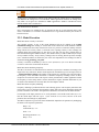
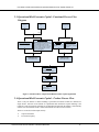
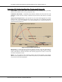
2.3. Operational Risk Economic Capital - Functional Process Flow
Diagram
INTERNAL LOSS
DATA
EXTERNAL LOSS
DATA
SCENARIO DATA
Scaling
SEVERITY MODELING
FREQUENCY MODELING
Poisson, Binomial, Neg-Binomial
Log normal, Emperical, EVT, Weibull,
Gamma, Exponential, Pareto,Burr, Gumbel,
Uniform, Log logistic, Log Gamma, Truncated
Burr, Truncated Exponential, Truncated
Gamma, Truncated Gumbel, Truncated LogGamma, Truncated Log-Logistic, Truncated
Log-Normal, Truncated Pareto, Truncated
Uniform, Truncated Weibull
FREQUENCY
MODELING
Poisson, Binomial, NegBinomial
COMPOUND LOSS
DISTRIBUTION – MONTE
CARLO SIMULATION
SEVERITY MODELING
Log normal, Weibull, Gamma,
Exponential, Pareto,Burr,
Gumbel, Uniform, Log logistic,
Log Gamma
COMPOUND LOSS
DISTRIBUTION – MONTE
CARLO SIMULATION
INSURANCE
-Deductible Model
-Proportional Retention Model
AGGREGATE LOSS
DISTRIBUTION
-VaR
-Conditional VaR
ALLOCATION
-Expected Loss
-Unexpected Loss
Figure 1: Functional Flow of Operational Risk Economic Capital Application
2.4. Operational Risk Economic Capital – Product Process Flow
There is only one dataset on which modeling is performed as business models are defined on a
single dataset. Selection of the dataset for Operational Risk Economic Capital modeling is not
required, as after choosing the technique (Loss Distribution Approach) the dataset is automatically
chosen. Once the business model is selected the dataset browser becomes invisible.
There are seven tabs for data input, namely:

Capital Calculation

Loss Data Frequency
Oracle Financial Services Software Confidential-Restricted
14
User Guide: Oracle Financial Services Operational Risk Economic Capital, Release 2.1

Loss Data Severity

Scenario Data

Credibility Factor

Data Transformation

Filter
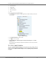
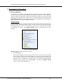
To access these tabs refer to the following steps:
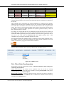
1.
Click Modeling on the LHS pane of OREC application (in sandbox infodom), shown in the
following figure:
Figure 2: OREC modeling
2.
Click Model Management to define a model.
3.
Click
4.
Enter the Model Name, Model Description, Technique, Model Objective in the Model
Definition screen.
to create a new model.
The seven tabs for data modeling are displayed and explanation of each tab is provided in the
following sections.
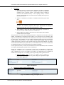
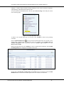
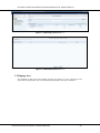
2.4.1. Tab.1: Capital Calculation
The inputs in Capital Calculation Settings tab are the inputs given before modeling. These are
mandatory fields to be updated for Operational Risk Economic Capital calculation. There are three
sections under the Capital Calculation Settings tab namely: Reporting Groups, Parameters,
and Options.
Oracle Financial Services Software Confidential-Restricted
15
User Guide: Oracle Financial Services Operational Risk Economic Capital, Release 2.1
Figure 3: Operational Risk Economic Capital Model Definition Screen

Reporting Group
Select the type of RG on which EC modeling is performed, that is, whether the modeling is
to be done on regulator prescribed Standard Reporting Group or on Internal Reporting
Group as specified by the bank. In the Reporting Group section Reporting Group
Relevance Setting should also be updated. OREC application supports processing on 56
RG’s or a selected group of RGs specified in the Relevance Setting Grid.
Figure 4: Reporting Group Relevance Setting Screen
The Reporting Group Relevance Setting remains disabled if the RG is not selected. If the RG is
changed before the model is saved, the frequency and severity tab parameters changes to null, if
there are any new LOB and ETs then the dimension table should be resaved in the hierarchy.
Oracle Financial Services Software Confidential-Restricted
16
User Guide: Oracle Financial Services Operational Risk Economic Capital, Release 2.1

Parameters

Reporting Currency: An entity having operations in multiple geographic
areas and those which have losses in multiple currencies, EC should be
calculated in the reporting currency. The historical losses should be
converted from standard currency to the reporting currency. Scenario
severity values should also be converted to the reporting currency prior to
the model execution.

Number of simulations: The number of simulations should be greater than
zero.
Severity Loss Simulation uses the temporary table space as a part of model
execution. The Database temporary table space requirement for running 56
Reporting Groups (RG) with 1,000,000 simulations is 12GB.

Time window (in days): The time window would specify the number of
days the loss data would be used for risk computation.

Bucket length: The length of the bucket as in the frequency data would be
calculated based on this length.
These parameters are used in the simulation generation of frequencies and severities. Enter the
number of simulations of frequencies and severities to be generated for loss calculation. The
inputs for these parameters should follow the validation rule. The input value for this field should
be greater than 1. The parameters for Time window and Bucket length are used to form the time
buckets (number of time buckets = Time window in days/ Bucket length). Each time bucket
contains the frequency of the loss event occurrence with respect to that particular RG. The number
of time buckets should always be greater than 3; else the model fails to save. This is further used
in calculating frequency in the relevant buckets for Frequency Modeling.
Use this option extensively to avoid errors like data does not follow distribution, data not available
for frequency modeling along with the choice of distribution.
Specify the confidence level for Economic Capital (EC) and Regulatory Capital (RC)
computation. Confidence level is ideally between 95% and 100%. However, RC for operational
risk is calculated at one rate, for example 97.5% and EC for operational risk is calculated at
another rate for example 99%. Accordingly, input any percentage values greater than zero.

Random number seed: A seed is a number used to initialize a
pseudorandom number generator. A positive integer is expected as an input
in the OREC application.
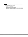
Figure 5: Parameters

Options in Capital Calculation Settings Tab:
Figure 6: Simulation Settings and Options Screen
Oracle Financial Services Software Confidential-Restricted
17
User Guide: Oracle Financial Services Operational Risk Economic Capital, Release 2.1
In this tab specify various conditions under which the simulations are to be done. Here you can
select the appropriate options depending upon the availability of external and scenario data.
Additionally you may or may not consider insurance.
You also have the option to Calculate Allocation Factor by selecting Yes in the available
options, after which OREC application generates the allocation factor. On the other hand, if
Calculate Allocation Factor is No then the factor is expected as a download. UL at the aggregate
level is distributed back to the RGs in proportion to the variances and co-variances of the
individual RG losses.
You can specify the Distribution Fitting Methodology as Maximum Likelihood Estimate (MLE),
Method of Moment (MM), or Maximum Likelihood Estimate (BFGS).
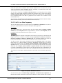
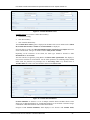
2.4.2. Tab.2: Loss Data Frequency
The loss data frequency has two sections namely- Correlation and Parameters. You have to
specify the copula method and correlation technique in OREC application.
Correlation:
The copula method has a drop down menu with four options namely Gaussian, Gumbel,
Student’s-t, and Not Required. When Copula Method is selected as Not Required, then the
Correlation field remains disabled and the Copula is not used.
Parameters:
The OREC application estimates the dependence between the RG frequencies of internal loss data
using any one of the correlation co-efficient techniques Spearman’s correlation co-efficient or
Pearson’s correlation co-efficient or Kendall’s Tau. The correlation technique to be used is to
be specified. Dependency is measured only for frequencies of the loss data across RGs.
You have to specify the frequency distribution selection and Tolerance Level in the adaptive
model. There are 5 options available in Frequency Distribution selection and any one can be
selected. The available options are Adaptive, Poisson, Binomial, Negative-Binomial and User
Specified. When any one of the first four options are selected then all the cells follow the selected
distribution that is adaptive, poisson, binomial or negative binomial. When adaptive distribution
is selected the distribution is selected based on the input data and the best fit distribution. The
decision for the best fit distribution for RG is done according to the mean and variance of the data.
The tolerance level for adaptive modeling should be a percentage value and should be greater than
zero.
Figure 7: Frequency Distribution Selection
You also need to specify the BEICF Shape Adjustment and BEICF Scale Adjustment. The
Business Environment and Internal Control Factors (BEICF) are those measures that are usually
Oracle Financial Services Software Confidential-Restricted
18
User Guide: Oracle Financial Services Operational Risk Economic Capital, Release 2.1
associated with the day-to-day operations which are high frequency or low impact (HFLI) events.
In contrast, the scenario data typically considers low frequency and high impact (LFHI)
operational events. In Frequency Modeling, the fitted distribution’s parameter like shape and scale
are calculated by Method of Moments or Maximum Likelihood. The parameters are rescaled to
represent a one year period. The parameters are multiplied by the number of time buckets in a year
to rescale the parameters. Rescaled parameters are adjusted for BEICF shape and BEICF scale
adjustments by multiplying the factors given as an input. This BEICF shape and scale adjustments
should be a value greater than zero and is used as a percentage increment to the calculated
parameters. In order to scale down the parameters the BEICF shape and scale should be less than
1.
For example: if the Shape parameter is 0.5 and BEICF shape adjustment is 10, then the adjusted
shape is 5.
You also have the flexibility to select the distribution for each cell by selecting the option User
Specified.
The inclusion of near miss data would be in the interest of the modeling analyst as its inclusion or
exclusion may change the capital calculation.
Near miss events would not have any severity value attached to it. Hence, they are considered only
for frequency modeling. The data needs to be passed to the NAG and shape and scale should be
considered as output.
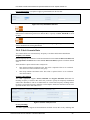
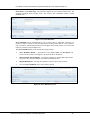
2.4.3. Tab.3: Loss Data Severity
Severity Distribution Selection: The available dropdown options are Empirical, Log Normal,
Extreme Value Theory (EVT), Weibull, Gamma, Exponential, Pareto, Burr, Gumbel, Uniform,
Log Gamma, Log Logistic, Truncated Burr, Truncated Exponential, Truncated Gamma, Truncated
Gumbel, Truncated Log-Gamma, Truncated Log-Logistic, Truncated Log-Normal, Truncated
Pareto, Truncated Uniform and Truncated Weibull. When any one of these options are selected
then all the 56 cells (or cells selected for processing) follow the selected distribution, but you also
have the flexibility to select the distribution of each cell by selecting the option User Specified. If
EVT is used as the distribution, then the modeling analyst has to specify whether to calculate the
EVT Threshold or to specify the threshold value. The specified EVT threshold value should
always be greater than 50%. EVT fitting is done after outlier treatment. Due to this if outlier is
opted for along with EVT, the threshold point may be of a smaller value than expected.
USER_CAPPING_SELECTION= “YES” with CAPPING_SHAPE_LOWER_VAL = -0.5 and
CAPPING_SHAPE_HIGHER_VAL= 1. This combination changes the fitted shape parameter of
distribution if it falls outside the range defined. Estimated values are replaced by the nearest
threshold value in case the range is breached.
USER_CAPPING_SELECTION= “FAIL” with CAPPING_SHAPE_LOWER_VAL = -0.5 and
CAPPING_SHAPE_HIGHER_VAL= 1. This combination changes the fitted or estimated shape
parameter of distribution if it falls outside the range defined. It also conveys that the Run would
fail if estimated parameters are outside range. You are required to change the data or redefine
buckets for improvement in parameter values.
USER_CAPPING_SELECTION= “NO” with CAPPING_SHAPE_LOWER_VAL = -0.5 and
CAPPING_SHAPE_HIGHER_VAL= 1. This combination changes the fitted shape parameter of
the distribution if it falls outside the defined range. In this option the OREC application performs
simulation even though the parameters are outside range. Simulation that results from such an
execution should be read with caution.
In all 3 cases you can modify the lower and upper values depending on the experience. However, 0.5 and 0.75 or 1 are standard values. As for shape parameter value of 1 and greater than or less
than -0.5, the distribution has infinite variance and simulated values are erratic. Apart from EVT,
there are 11 other options available in severity distribution selection, and any 1 can be selected.
Oracle Financial Services Software Confidential-Restricted
19
User Guide: Oracle Financial Services Operational Risk Economic Capital, Release 2.1
Log Transformation: is an option to apply log transformation on the loss data.
Figure 8: Severity Distribution Selection
If the severity distribution specified is user specified and EVT is selected at grid level, then input
different EVT Threshold at grid level for different RG’s or specify one EVT Threshold % for all
the RG’s.
The RGs which are not selected for processing from the Reporting Group Relevance Settings
field are disabled from selecting distribution.
2.4.4. Tab.4: Scenario Data
The scenario tab has two sections namely- Frequency Correlation and Scenario Distribution:
Frequency Correlation:
In this tab specify the Correlation Coefficient Estimation between Use Loss Data Correlation and
User Specified Correlation. Based on Use Loss Data Correlation, input the correlation default
value.
There should be 2 inputs in the Scenario Analysis tab:

Inter Scenario Default Correlation Value: This value is replaced if there is no correlation
value between scenarios within the same group.

Inter Group Default Correlation Value: This value is replaced if there is no correlation
value between RGs.
Frequency Distribution:
The OREC application supports Poisson, Binomial and Negative Binomial distribution for
modeling frequency of scenario data. In this tab you need to specify the Frequency Distribution
and Scenario Distribution. The list of distributions for scenario data frequency modeling follows
the same as in loss data frequency modeling. For the adaptive model, the tolerance level has to be
specified and this can be done at RG level.
Figure 9: Scenario Analysis Screen
Severity Modeling:
The OREC application supports all the distributions available for loss data severity modeling with
Oracle Financial Services Software Confidential-Restricted
20
User Guide: Oracle Financial Services Operational Risk Economic Capital, Release 2.1
the exception of Extreme Value Theory (EVT), Empirical and Truncated distribution.
Since, EVT is best applicable for the data with extreme deviation from the mean it is the outcome
of user judgment based on the risk and control assessments within the bank and the scale of
operation. This peculiarity of the scenario data makes it difficult to fit Empirical distribution.
Since, EVT approach comprises of Empirical distribution and Generalized Pareto distribution, it is
not advisable to fit EVT to scenario data. Log Normal, being a skewed tail amongst all thin-tailed
family of distributions, proves to be the best distribution for scenario data. The mode and
percentile given as a download for specific reporting groups are used to fit a Log Normal
distribution to the scenario data. The process outputs calculated are stored in OREC application
Process_Output table.
OREC application supports two different approaches for modeling severity data:
Formula Based: Usage of formula for severity modeling.
Bound Data: Bound data approach follows modeling similar to severity modeling of loss data.
The convention between Formula based and Bound data can be handled in tool matrix.
Scenario data can also be defined at reporting group level by User Specified option available
under the pane.
When scenario data is specified as No in the Capital Calculation tab; the Scenario Data tab will
be disabled. Default correlation value is used only when loss data correlation is used.
2.4.5. Tab.5: Credibility Factor
You have to define two parameters, the first one being the credibility approach for scenario
analysis method where Alternative, Complimentary, Aggregate or User Specified should be
selected. The second parameter is the credibility factor.
For example: At the bank level if the number of simulations is 10000, then there would be 10000
loss simulations and 10000 scenario simulations. These 20,000 simulations have to be converted
to a final set of 10000 simulations. In other words, internal or external simulations have to be
combined with scenario simulations, for which three methods alternative, complimentary and
aggregate are available.
Under Alternative method, given the credibility factor as 30%, 30% of worst severities of scenario
simulations replace the corresponding simulated losses of internal or external data. It should be
noted that ordering simulated losses may be necessary as worst scenario simulations has to replace
the worst internal or external simulations.
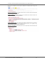
0% credibility factor would mean only internal or external simulations will be considered for risk
measure estimation.
Credibility-30%
Simulation
Number
1
Loss
Simulation
983,251.02
Scenario
Simulation
180,498.51
Alternative
method
983,251.02
Complimentary
method
983,251.02
Aggregate method
2
1,138,076.71
197,034.75
197,034.75
1,138,076.71
1335111.46
3
1,033,025.97
205,420.06
205,420.06
205,420.06
1238446.03
4
993,809.59
232,148.67
232,148.67
993,809.59
1225958.26
5
1,106,787.55
183,942.18
1,106,787.55
1,106,787.55
1290729.73
6
861,358.99
157,605.63
861,358.99
157,605.63
1018964.62
7
922,687.69
136,863.81
922,687.69
922,687.69
1059551.5
Oracle Financial Services Software Confidential-Restricted
1163749.53
21
User Guide: Oracle Financial Services Operational Risk Economic Capital, Release 2.1
Credibility-30%
Simulation
Number
8
Loss
Simulation
849,574.94
Scenario
Simulation
139,645.23
Alternative
method
849,574.94
Complimentary
method
849,574.94
Aggregate method
9
971,087.05
164,617.35
971,087.05
164,617.35
1135704.4
10
869,749.37
177,235.19
869,749.37
869,749.37
1046984.56
989220.17
Table 8: Credibility Factor
In the complimentary approach, random replacement of internal or external simulations is done by
randomly picking simulations from scenario data depending upon the credibility factor. Random is
the key here.
100% credibility factor would mean only scenario simulations are considered for risk measure
estimation. Again 0% and 100% credibility factor can also be achieved. While calculating bank
level VaR it does not consider worst cases from both sides and also does not ignore the tail
portion. This is done by preserving the simulation order which ties the frequency generation done
for all RGs. It is preserved as OREC application uses copula to generate frequency so that real
data is imitated as much as possible.
For example: let’s assume that there are 10 simulations from loss data and 10 from scenario, all
tied together by the simulation order. If the first simulation number itself is the worst case for the
scenario then OREC application ignores loss simulation. It does not check if ignored loss value is
worst case or not. This results in Diversified VaR which applies portfolio effect to RG
combinations by preserving the relationship generated by copula.
Under aggregate method loss simulation values are summed up with scenario simulations values.
For example: if there are 10000 loss simulations and 10000 scenario simulations, then total
number of simulations by aggregate method is 20000 simulations.
When scenario data is specified as No in the capital calculation tab; the Credibility tab will be
disabled. Default correlation value is used only when loss data correlation is used.
Figure 10: Credibility Factor
2.4.6. Tab.6: Data Transformation
The parameters in the data transformation include - outlier determination, outlier scaling factor
and missing value treatment.
Outlier Determination: The outliers can be identified across all the RGs by selecting
Interquartile Method or can be made across each RG by selecting User Specified or this process
can be excluded by selecting Not Required.
Missing Value treatment: 3 options to replace the missing value in the loss data are available by
the Mean of the data or you can Omit the data or customize the selection at the RG level by
selecting the User Specified option.
Oracle Financial Services Software Confidential-Restricted
22
User Guide: Oracle Financial Services Operational Risk Economic Capital, Release 2.1
Figure 11: Data Transformation
2.4.7. Tab.7: Filter
Add multiple Hierarchy members as filters, as shown in the screen. Select filter tab in the Model
Definition New screen. This is mainly used for entity selection.
Figure 12: Filters
2.5. Stress Testing Overview
The Stress Testing Framework has four parts:

Variable definition

Shock library

Scenario definition

Stress definition
Variable Definition: Stress Testing allows the bank to conduct an analysis that enables it to
estimate the impact of movements in the variables on measures such as profitability, capital
Oracle Financial Services Software Confidential-Restricted
23
User Guide: Oracle Financial Services Operational Risk Economic Capital, Release 2.1
adequacy. A what-if analysis enables strategic planning in areas such as customer acquisition,
capital planning, fund management and many more.
To access the Stress Testing framework, click the option Stress Testing in the LHS pane, shown
in the following figure:
Figure 13: Variable Definition Selection
To define a new variable which has to be stressed, select Variable as shown in the preceding
screenshot.
In the Variable Definition New
screen, the name and description of the new variable is to be
defined. Enter a suitable name and description of the new variable in the Variable Name and
Variable Description fields respectively. From the Variable Type dropdown list select
Idiosyncratic Variable.
Based on the drop-down list, select Measure to create a variable based on Measure. The Variable
Set Management pane is displayed on the RHS of the screen.
Figure 14: Variable Management Screen
Details such as Variable ID, Variable Name and Creation details are displayed. In the Variable
Definition New screen the name and description of the new variable is to be defined.
Oracle Financial Services Software Confidential-Restricted
24
User Guide: Oracle Financial Services Operational Risk Economic Capital, Release 2.1
Figure 15: Variable Definition Screen
Variable Shock: To access the Variable Shock Library:
1.
Click Stress Testing.
2.
Click Shock Library
3.
Click Variable Shock library.
The Variable Shock Library pane is displayed in the RHS of the screen. Details such as Shock
ID, Variable Shock Name, Variable and Creation Details are displayed.
Select the data set, in this case Operational Risk Economic Capital Process Output and browse
for the variable name. The type of variable would be Idiosyncratic Variable.
Depending on the occurrence of the shock, the shock type should be defined as either
Instantaneous or Across Time.
The filter can also be applied by using New in the Shock Filter Specification. This displays a
new browser with the list of hierarchies. For the shock parameter, the modeling analyst should
either shock the parameter on percentage base as Percentage shift or by absolute base as
Absolute Shift. The values of the shift should be defined at the Shock value.
Figure 16: Variable Shock Definition
Scenario definition: A Scenario is a set of multiple Variable shocks and Rule shocks. These
shocks may be Rule Based Shocks or Variable Based Shocks. You can define a Scenario using a
combination of Rule Based Shocks and Variable Based Shocks.
Navigate to New Scenario Definition, which displays a new browser with Variable Name,
Oracle Financial Services Software Confidential-Restricted
25
User Guide: Oracle Financial Services Operational Risk Economic Capital, Release 2.1
Shock Name, and Variable Type. This would also display the list of shocks defined earlier. The
selection of multiple shocks together forms a new scenario. This combination results in a New
Scenario name.
Figure 17: Scenario Definition
Stress Definition: Stress Definition allows you to specify either a stand-alone execution of a
Scenario or maps a Scenario to a Baseline Run, thereby creating a Stress Run. It is also possible to
map a Scenario to multiple Baseline Runs. This integrated stress testing enables you to assess the
impact of a Scenario across multiple areas.
The Stress Definition New screen contains three panels namely:

Stress Definition Details – Specification of the Stress Name and Description and
selection of the scenario to be mapped to the particular Stress Definition.

Model-Variable Shock Mapping - Viewing the mapping of Variable Based Shocks that
form part of the selected scenario to the models in the Baseline Run.

Mapped Rule Shocks - Viewing rules and their respective shocks from scenario.

The saved Stress definition can be either edited or deleted.
Figure 18: Stress Definition Screen
Oracle Financial Services Software Confidential-Restricted
26
User Guide: Oracle Financial Services Operational Risk Economic Capital, Release 2.1
Oracle Financial Services Software Confidential-Restricted
27
User Guide: Oracle Financial Services Operational Risk Economic Capital, Release 2.1
3. Preparing for Execution
3.1. Set up definition
Set up pertains to the ability of OFSAAI platform to calculate loss values. OREC application
provides two such infodoms namely Sandbox and Production. Sandbox is a sort of trial area.
Various combinations of parameters can be tested till the desired results are achieved. The model
output can then be deployed after which it can be accessed in production. In production, the
Model Management option is not available which restricts the changing of the model parameters.
However, this can also be achieved through the sandbox.
Sandbox Definition
Within modeling environment (Sandbox Environment), data would be extracted or imported from
production infodom based on the dataset defined. Also, this can be the first data movement from
the staging to the FACT table as well. The objective of this step is to fetch data for all attributes
for a particular time period. The Sandbox Definition screen is reproduced below for easy
reference:
Figure 19: Sandbox Definition
Sandbox Definition Screen includes the following:

Model Management
Before model definition, LOB & ET Reclassification needs to be performed. The LOB and
ET information is either reclassified according to the regulator rules or according to the
bank’s own reclassification rule. Oracle Financial Services Operational Risk Economic
Capital, Release 2.1, Calculation is a business model. You should select Operational Risk
Economic Capital modeling from the Technique screen under the Business Models
category as shown in the following screen:
Oracle Financial Services Software Confidential-Restricted
28
User Guide: Oracle Financial Services Operational Risk Economic Capital, Release 2.1
Figure 20: Operational Risk Economic Capital Modeling: Business Model Browser
Defining Operational Risk Economic Capital Model in Modeling Framework (MF):
Provide data input for the calculation of Operational Risk Economic Capital. Input the
Model Name, Model Objective and Technique for modeling (in Business Models Loss
Distribution Approach is selected).
Model Name: Loss Distribution Approach
Model Description: Operational Risk Economic Capital Estimation for Standard RG with
Financial Services and Scaled External Data.
Model Objective: Portfolio Operational Risk EC Estimation
Technique: Operational Risk Economic Capital Modeling

Model Execution
After OREC application model is defined, request for execution is made. The Model
Execution is available at the bottom of the screen. Using this option, a message Model
Execution Triggered is displayed. The execution of the model requires the MIS date and
the number of executions to be greater than zero.

Model Output
For more information on Model Output, refer to Operational Risk Economic Capital
Reporting on page 32.

Model Deployment
You can deploy the model in the production infodom and execute it. However, in the
production infodom an end-to-end process to execute the Operational Risk Economic Capital
model should be defined.
Screenshots relating to model deployment are as follows:
Oracle Financial Services Software Confidential-Restricted
29
User Guide: Oracle Financial Services Operational Risk Economic Capital, Release 2.1
Figure 21: Model Deployment Screen – 1
Figure 22: Model Deployment Screen – 2
3.2. Staging Area
The uploading of data involves the loading of all the stage tables. For more information on the
stage tables to be populated, refer to the Download Specifications (DL Specs) documents.
Oracle Financial Services Software Confidential-Restricted
30
User Guide: Oracle Financial Services Operational Risk Economic Capital, Release 2.1
4. Execution
A Run is executed in the production infodom to calculate Operational Risk Economic Capital. A
Run in the production infodom consists of the following:

T2T: Stage to FACT Table data loading.

Reclassification Rules: These are Rules to reclassify Internal to Standard, External to
Standard, External to Standard LOB and Standard ET.

Model Execution: Models defined in the sandbox are re-executed through a Run in the
production infodom.
For more information on execution of a Run, refer to the Technical Metadata Worksheets.
Oracle Financial Services Software Confidential-Restricted
31
User Guide: Oracle Financial Services Operational Risk Economic Capital, Release 2.1
5. Operational Risk Economic Capital Reporting
A reporting dashboard is also provided with the OREC application. This involves a combination
of graphical as well as tabular reports. You are provided with report filters to view data in different
ways.
A model run using Run execution is all that the dashboard needs. The dashboard queries the same
database using filters like Run descriptions, execution date and so on.
Graphical reports:

OR Risk Loss Distribution

Risk Measures Across Time

Internal Loss Statistics

Economic Capital Allocation to Lines of Business

Economic Capital Allocation to Event Types

Line of Business Analysis




Key Risk Measures

Economic Capital Trend

Loss Event Statistics

Economic Capital Allocated to Event Types

Loss Frequency Analysis

Loss Severity Analysis
Event Type Analysis

Key Risk Measures

Economic Capital Trend

Loss Event Statistics

Economic Capital allocated to Event Types

Loss Frequency Analysis

Loss Severity Analysis
Analysis across Models

Risk Measures across Models

Model General Details
Simulation Reports

Simulated Values of Frequency for Scenario Data

Simulated Values of Severity for Scenario Data

Simulated Values of Aggregated Loss for Scenario Data

Distribution Parameters

Stress Testing
o
OR Loss Distribution
o
Risk Measures across Time
Oracle Financial Services Software Confidential-Restricted
32
User Guide: Oracle Financial Services Operational Risk Economic Capital, Release 2.1
o
Economic Capital Allocation to Line of Business
o
Economic Capital Allocation to Event Types
o
Frequency Shape and Scale Analysis for Event Type
o
Severity Shape and Scale Analysis for Event Type
The following reports need to be calculated both for Standard RG (combination of Standard LOB
by Standard ET) as well as Internal RG (combination of Internal LOB by Internal ET). For
example: if a bank has 10 Internal LOB and 3 Internal ET then the number of Internal RGs would
be (10 * 3) 30. However, for reporting purposes, the number of Standard RGs would be (8 * 2) 16
(where 2 of the Internal ETs map to 1 Standard ET). Operational Risk Economic Capital generates
the following 43 reports.
Tabular Reports

OR Dependency Matrix Correlation Value - Standard

OR Dependency Matrix Covariance Value - Standard

OR EC Across Internal Event Type

OR EC Across Internal Line of Business

OR EC across Internal Reporting Groups

OR EC Across Standard Event Type

OR EC Across Standard Line of Business

OR EC across Standard Reporting Groups

OR Goodness of Fit Statistics for Internal Reporting Group

OR Goodness of Fit Statistics for Standard Reporting Group

OR Key Stats for Internal Data - Internal Reporting Group

OR Key Stats for Internal Data - Standard Reporting Group

OR RC Across Internal Event Type

OR RC Across Internal Line of Business

OR RC across Internal Reporting Groups

OR RC Across Standard Event Type

OR RC Across Standard Line of Business

OR RC across Standard Reporting Groups

OR Key Stats For External Loss - INT RG

OR Key Stats For External Loss - STD RG

OR Key Stats of Int and Scaled Ext Loss-INT RG

OR Key Stats of Int and Scaled Ext Loss-STD RG

OR Dependency Matrix Correlation Value – Internal

OR Dependency Matrix Covariance Value - Internal
Oracle Financial Services Software Confidential-Restricted
33
User Guide: Oracle Financial Services Operational Risk Economic Capital, Release 2.1
Frequently Asked Questions
1.
How is EVT calculated by OREC Application?
OREC application segregates the loss data as per given time buckets. For this time bucket, mean
and variance is calculated. OREC application begins with 50% value of loss data. Only those loss
values are chosen which falls above the threshold point. These newly found values are again
segregated in time buckets. OREC application then checks if mean is greater than variance for this
data. The same process is repeated with a jump of 1% till mean is greater than variance. The upper
threshold of percentile is 99.9%
While calculating monetary value of threshold point, OREC application follows the function
similar to percentile in Microsoft Excel. This helps in finding the exact percentile value and results
in a threshold value which may not be a part of loss data.
2.
How does OREC application calculate the outlier?
OREC application calculates outlier by using Inter Quartile method. This is done to find out those
data points which divide the data (in a sorted manner) in 4 equal parts. Thus, data points which are
at 25%, 50% and 75% percentile of the data are required.
However, in this case, OREC application follows cumulative percentile calculation for each data
point to find the correct value. Due to this approach, quartile points are always part of the loss data
and thus they are approximately 25%, 50% and 75%.
3.
How are VaR numbers calculated?
VaR algorithm attempts to retain the respective weightage of various RGs with respect to each
other when frequency for each RG is simulated. Due to this when simulated losses are summed
across the RGs to get bank level VaR it avoids forming simultaneous peaks for each RG. This
peculiar structure results in diversified VaR.
4.
Is model execution in Sandbox a compulsory step?
Sandbox is a trial area. You can define various models and analyze the output. Once the model is
defined as per business requirement, deploy the same for production set up. If you are certain
about the model execution results then deploy the same directly.
However, it is advised to go through the sandbox as execution errors (data non availability, choice
of distribution) will be eliminated following this step.
5.
How to find which distribution fits the data properly?
To begin with, for frequency analyses select the adaptive method. In this method, OREC
application chooses the method which is more suitable for the data. When it comes to severity
analysis, use the Modeling Framework (Platform) to get statistics regarding Goodness of Fit for a
given data under various methods.
6.
Why do we get copula failure errors?
Copula works mainly on correlation values between RGs. There are a few obvious reasons for
copula failure which are as follows:
Erroneous insertion of data under User Specified resulting in correlation value <-1 or >1.
Matrix approach is not followed.
For example: RG (ET-2, LOB-3) has correlation value of 0.5 but (LOB-3, ET-2) has been inserted
as 0.6. When Gumbel Copula is, the correlation values are to be restricted between 0 and 1 as here
non zero and positive values are required.
7.
Why we get error “Data does not follow … distribution” error? And how can we overcome this
error?
Oracle Financial Services Software Confidential-Restricted
34
User Guide: Oracle Financial Services Operational Risk Economic Capital, Release 2.1
Every data has its own characteristic which is suitable for a particular distribution or class of
distribution. For example: when mean is equal to variance Poisson is used. If we try to fit the data
which does not follow a particular distribution, we end up doing a force fit which may lead to
errors.
Another reason can be the choice of buckets. Frequency modeling depends on bucketing. Change
in the bucket window and time period can substantially alter the data characteristics. It is advised
to choose a correct bucket structure for the output to match the expectation. However, it is always
advisable to go though the Modeling Framework which provides a lot of tools like Goodness of
Fit to judge the fit.
8.
Do I need to re-execute the Runs for reports?
Additional executions for reporting purposes are not required. Refer to the Run executed in the
batch execution area along with execution date, and access the required report. Additional runs
after batch execution are not required to be executed even if you are using the dashboard or not.
Dashboards can be linked to either sandbox or production set up.
9.
How does a Random Number Seed function?
Simulation programs make use of a pseudorandom number generator that requires a seed. If none
is provided, a System Generated seed will be used. This is used to separate the different
simulations within a single run. Any positive integers can be a random seed.
10. Which are the hierarchies on which I can apply the filter?
In model definition, OREC application provides a wide range of hierarchies on which filters can
be applied. You have a choice of selecting those hierarchies that form a part of OREC modeling
data set.
11. How will the outlier scaling factor be used and what would be the range for the same?
Outlier is used to identify those data values which should logically be a part of tail ends. OREC
application provides inter quartile method for this. Q1 and Q3 are inter quartile ranges
Upper Hinge = Q1 – K*(Q3 –Q1)
Lower Hinge = Q3 + K*(Q3 –Q1)
K is outlier scaling factor. Higher values of K widens the range and vice versa. There are no
common values for this. However, outlier scaling factor of 1 reduces the range to inter quartile
range. Values less than 1 are not advisable.
12. When does model version change and when is the model asked to be saved with a different
name?
Model changes can be saved in two ways. First, called version change involves minor changes like
simulation numbers, bucket parameters, random number seed, and insurance percentage. Changing
these parameters is not considered as the one which impacts the basic structure of the model and
hence the same can be saved with the new version number.
However, if any other changes are made, ensure that you save it as a new model as all other
changes impact the modeling structure.
13. Where will I find outlier and missing value treatment results for view?
The relevant files are saved in the following location:
…/home/RORECst/ftpshare/INFODOM/scripts/modeldatafiles
Infodom values are generally RORECSAND or RORECPROD depending on which infodom the
Run or model is executed on.
14. Why is external data used only for severity modeling?
External loss data is not utilized for modeling of frequency as it is characterized by low frequency
Oracle Financial Services Software Confidential-Restricted
35
User Guide: Oracle Financial Services Operational Risk Economic Capital, Release 2.1
and high severity data and therefore is considered only at the time of modeling severity.
15. How do I select between formula based and bound method for scenario severity modeling?
You can make changes in the tool matrix XML file which are valid across models and users which
indicate that changes made here will have a global impact.
16. How does log transformation help?
Log transformation helps in variance stabilization. Increasing slopes in X in relation to another
variable are linearized. Positively skewed distributions of X are normalized.
17. Where do we set threshold values for external loss data?
In the Rules framework you can specify upper and lower thresholds of external loss data. Later,
outlier can be applied to ensure data selected for modeling resembles the expectations set or
business requirements.
18. For OBI reports (Dashboard) is execution compulsory in production set up?
OREC application provides the option to generate OBI reports from Sandbox or Production set up.
This is handled in OBI settings. If sandbox is selected from OBI then Run in production set up for
OBI need not be executed. However, by default the choice provided in OREC application setting
is Production.
Oracle Financial Services Software Confidential-Restricted
36
User Guide: Oracle Financial Services Operational Risk Economic Capital, Release 2.1
Annexure A: Things to Remember
Frequency Modeling - If you are unaware of the distribution type of the data for each RG, select
Adaptive modeling so that OREC application models on its own and selects the relevant
distribution type for each RG to calculate the frequency parameters. Near miss values are optional
and included only in frequency modeling as they do not hold any severity values. Tolerance level
as per industry standards given as a user input should normally be between 1% and 5%. BEICF
adjustments should be in percentage value and is given as a decimal value input.
External Data- External data and Scenario data are not subject to any outlier adjustments.
Near Miss- Near miss values are excluded from any missing value transformations.
Scenario Data- Scenario data is independent of time bucket definition as the frequency and
severity data is obtained directly as a download. This data is directly used for shape and scale
determination. Scenario data does not undergo log transformation.
Dependency Between Loss Frequencies - Dependency is measured only for frequencies of the
internal loss frequency data across RGs.
Time Bucket Input - The ratio of Time Window and Time Bucket Length should be greater
than 3, failing which the model will not be saved.
Severity Modeling- EVT is best applied for data with extreme deviations from the mean or
technically the data with fat tail.
Insurance –Insurance data should be mandatorily provided (EEL and Agg Data), if Consider
Insurance is updated as Yes in Capital Calculation Settings Tab.
Ideally, the EEL deductible amount or the EEL percentage (in case of Proportional Model) should
be given as a download. Else, Net EEL claim = Loss Amount.
All contract ID's in an RG should have EEL Deductible Amount or Aggregate Deductible Amount
if the insurance model is a Deductible Model. For a Proportional Retention Model, the
percentage for EEL and Aggregate Loss should be given, if deductible amount is not given.
Loss Calculation - If the sum of EC values at RG level is not equal to that at bank level, then
check the Variance - Covariance matrix to confirm.
Oracle Financial Services Software Confidential-Restricted
37
User Guide: Oracle Financial Services Operational Risk Economic Capital, Release 2.1
Annexure B: Understanding Key Terms and Concepts
Value-at-Risk - Value at Risk (VaR) is the maximum loss not exceeding a given probability
defined at the confidence level, over a given period of time.
Conditional Value-at-Risk – Conditional Value-at-Risk is defined as the mean of the loss α-tail
distribution. CVaR is derived by taking a weighted average between the VaR and losses exceeding
the VaR.
Expected and Unexpected Loss - The expected loss is the mean annual aggregate loss, and the
unexpected loss is the annual aggregate loss in excess of this mean, up to a particular confidence
level (say, 95 or 99 per cent confidence). The following diagram gives a detailed explanation of
Expected and Unexpected loss:
Figure 23: Expected and Unexpected Loss
Data Model- is a logical map that represents the inherent properties of the data independent of
software, hardware or machine performance considerations. The data model consists of entities
(tables) and attributes (columns) and shows data elements grouped into records, as well as the
association around those records.
Dataset - It is the simplest of data warehouse schemas. This schema resembles a star diagram.
While the center contains one or more FACT tables, the points (rays) contain the dimension tables
as represented in the following diagram:
Oracle Financial Services Software Confidential-Restricted
38
User Guide: Oracle Financial Services Operational Risk Economic Capital, Release 2.1
Dimension Table
Dimension Table
Products
Time
Geography
Sales
Fact Table
Customer
Channel
Figure 24: Data Warehouse Schemas
Metadata – A term used to denote data about data. Business metadata objects are available in the
form of Measures, Business Processors, Hierarchies, Dimensions, Datasets, Cubes, and so on.
The commonly used metadata definitions in this User Guide are Hierarchies.
Star Schema: In a star schema, only one join is required to establish the relationship between the
FACT table and any one of the dimension tables which optimizes queries as all the information
about each level is stored in a row. The set of records resulting from this star join is known as a
dataset.
Hierarchy – A tree structure across which data is reported is known as a hierarchy. The members
that form the hierarchy are attributes of an entity. Thus, a hierarchy is necessarily based upon one
or many columns of a table. Hierarchies may be based on either the FACT table or dimensional
tables.
Measure - A simple measure represents a quantum of data and is based on a specific attribute
(column) of an entity (table). The measure by itself is an aggregation performed on the specific
column such as summation, count or a distinct count.
Business Processor – This is a metric resulting from a computation performed on a simple
measure. The computation that is performed on the measure often involves the use of statistical,
mathematical or database functions.
Advanced Analytical Infrastructure – The Oracle Operational Risk Economic Capital Modeling
Environment performs estimations for a given input variable using historical data. It relies on prebuilt statistical applications to build models. The framework stores these applications so that
models can be built easily by business users. The metadata abstraction layer is actively used in the
definition of models. Underlying metadata objects such as Measures, Hierarchies, and Datasets are
used along with statistical techniques in the definition of models.
Additional Things to Remember:
The current version of OREC application supports two different approaches for modeling Scenario
Severity.
Bound Based: During this approach, the severity data is modeled similar to those of loss data. The
dropdown consists of all the distributions of severity distribution except EVT and Empirical.
Formula Based: Usage of this approach, the scenario data is modeled with respect to the available
formula. The conversion of formula based approach to bound based can be done in a tool matrix;
the resulting effects can be viewed in the front end for scenario data severity.
Tab Level Validation: UI can be modified for tab level validation or model level validation.
Oracle Financial Services Software Confidential-Restricted
39
User Guide: Oracle Financial Services Operational Risk Economic Capital, Release 2.1
During tab level validations, the value input is validated for its feasibility before moving to the
next tab.
Insurance Allocation Factor: If insurance allocation factor is selected as Yes, then the allocation
percentage is expected as a download.
Number of Buckets: The number of buckets for the simulated values should be edited in the
config xml. Refer to the screen shot pasted below:
Populate Simulation Table: The simulated values should be populated based on the settings in
the config. If this is remarked as Yes, then the simulated values will be updated in fct_
Operational Risk Economic Capital _simulation table.
Hierarchy code dropdown: The hierarchy filter code for internal and external classification has
to be specified in config xml.
Oracle Financial Services Software Confidential-Restricted
40
User Guide: Oracle Financial Services Operational Risk Economic Capital, Release 2.1
Annexure C: Error Messages and Observations
Error Messages: Functional Error Messages that may appear in OREC application are displayed
in the following table. Through this table any additional help or suggestive actions to be taken
when an error is displayed is provided:
MSG
IDENTIFIE
R
12
MSG DESCRIPTION
Suggested Action for End user
Error: Login Failed for
Check the login name and password.
220
143
Time Bucket Generation Failed:
No Time Bucket found
Frequency Modeling Failed
225
Could Not Fetch Data
Ensure that time buckets are defined properly and data falls
within these time buckets.
This mainly occurs as data does not follow distribution. This
is usually seen as a very large or negative parameter value or
inability to estimate them as well. Check the distribution and
time buckets.
However, sometimes this error may be displayed due to data
irregularities or if data exists but does not comply with the
time buckets.
This may be due to failure of connection to database.
226
No Data Returned by Query
227
Frequency Modeling: Number
of Data Points is less than 5.
OFSAA Frequency Modeling
Module requires minimum 5
data points
Frequency Modeling: Failed to
Compute Mean and Variance in
Adaptive Method Selection
228
230
Frequency Modeling: Failed to
Compute Number of Trials
231
Frequency Modeling: Number
of Trials cannot be Negative
232
Frequency Modeling: Failed to
Compute Number of Failures
Frequency Modeling: Number
of Failures cannot be Negative
Frequency Modeling: Unable to
estimates the Parameters for the
Fitted Distribution within
permissible range.
Frequency Modeling: Variance
is Zero, so the Data cannot be
fitted for the Distribution Type.
Failed to calculate EDA Outputs
in Frequency or Severity
Modeling
233
234
235
237
Since one or more filters applied does not return any data
check, the model definition, and data as well.
Frequency modeling needs minimum five data points
(buckets). If not present, the model fails. Check the data and
time buckets defined.
This mainly occurs as data does not follow distribution. This
is usually seen when there is a very large or negative
parameter value or inability to estimate them as well.
Check the distribution and time buckets.
This means in case of Negative Binomial or Binomial the
OREC application is unable to calculate N.
Check if distribution selected, data and time buckets are
defined.
This means in case of Negative Binomial or Binomial N is
negative. Check if distribution selected, data and time buckets
are defined.
Check if distribution selected, data and time buckets are
defined.
Check if distribution selected and data is proper and time
buckets are well defined.
This mainly arises due to force fitting. Check the distribution
selected or modify the time bucket definition.
When all the data points are of the same value, variance will
be zero. Check or modify the data as well as time buckets
defined.
Failure of statistics like Mean, Variance, Kurtosis and
Skewness for either frequency or severity modeling.
Review the data, Goodness of Fit and how good the fit is.
Oracle Financial Services Software Confidential-Restricted
41
User Guide: Oracle Financial Services Operational Risk Economic Capital, Release 2.1
MSG
IDENTIFIE
R
241
MSG DESCRIPTION
Suggested Action for End user
Goodness of Fit test failed
Failure of goodness of fit test indicates that data does not
follow the specified distribution.
Check or alter the distribution selected or time buckets.
242
After BECIF adjustment, Scale
Parameter ( Probability) is not
within the range 0 to 1
Failed to generate the CSV
Report file.
Mean cannot be Null or Zero for
the given distribution
The mean cannot be less than
variance for the given
distribution type
The Mean or Variance cannot
be null or zero
The mean cannot be greater than
variance for the given
distribution type
The Data is not following the
given Distribution Type
Check or modify BEICF parameters.
Variance is zero, so the data
cannot be fitted for the given
Distribution Type
Relevant Event Type or LOB
Data not found in the
Dimension tables.
At any given percentile data
doesn't follow specified
distribution. The data is not
constant as per EVT modeling
This happens if all the data points have the same numerical
value. Check the data points.
243
244
245
246
247
248
249
250
251
254
255
256
257
258
No Relevant RGs have data.
Cannot proceed further
Input values for Scenario
Severity Modeling cannot be
Null or Zero
Parameter percentile value in
formula based approach is less
than 4. Hence calculation for
Log Normal Distribution has
failed
Parameter percentile value and
median value in formula based
approach cannot be same
Parameter percentile value in
formula based approach is 0 or
1. Hence calculation for Weibull
or Exponential Distribution has
Check write permission on specified folders.
Review the data points for further actions.
Review the data points or distribution selected for further
action.
Review the data points for further action.
Review the data points or distribution selected for further
action.
This is usually seen as very large or a negative parameter
value or inability to estimate them.
Check the distribution and time buckets.
Check the LOB / ET dimension table.
This happens when you select Calculate for EVT threshold. If
at any percentile value Mean is not greater than or equal to the
Variance this message is displayed.
Either change the buckets or select Specify EVT threshold
option. While specifying the threshold value it should be
above 50%.
Self Explanatory
Update stage scenario data and scenario severity details as
required.
Provide percentile value as greater than 4.
Self Explanatory
Self Explanatory
Oracle Financial Services Software Confidential-Restricted
42
User Guide: Oracle Financial Services Operational Risk Economic Capital, Release 2.1
MSG
IDENTIFIE
R
MSG DESCRIPTION
Suggested Action for End user
failed
260
262
263
264
265
266
269
270
271
272
273
274
275
277
EEL Threshold is less than EEL
Deductible.EEL Threshold has
to be greater than EEL
Deductible Amount
Aggregate Threshold is less than
EEL Deductible.EEL Threshold
has to be greater than Aggregate
Deductible Amount
The Correlation Matrix is a Zero
Correlation Matrix. This type of
matrix is not valid
The given data does not suffice
the condition to form a
Correlation Matrix
Self Explanatory
The Correlation Matrix is not
available even though the Loss
Data is available for it.
Unable to convert the Semi
Definite of the User Specified
Loss Correlation Matrix
Failed to convert Semi Definite
of the Loss Correlation Matrix
Failed to convert Semi Definite
of the Scenario Correlation
Matrix
Negative association between
the RG's. Hence Gumbel Copula
failed
The correlation value between
RG's is greater than 1. Hence
Gumbel Copula failed
Correlation value between the
RG's cannot be 1 or more than 1
Theta computed is less than 1.
Hence Gumbel Copula failed.
Update the stage dependency matrix for the correlation value.
The correlation matrix is null.
So the theta cannot be
computed.
Copula could not be generated
for the given Copula type
Self Explanatory
Check correlation value in the dependency matrix table.
Check for the condition if values are not uploaded.
When RG1 say ET-3, LOB-4 has correlation value of 0.5 then
matrix approach requires that LOB-4, ET-3 also has value 0.5.
If this is not the case then matrix preparation fails.
Also if data has 4 RGs and correlation data is available only
for 3 RGs then the matrix generated will not suffice.
Check or modify the correlation values.
For (Gumbel) copula, non-zero positive values of correlation
are required. Update the same in the dependency matrix table.
For Gumbel copula, non-zero positive values of correlation
are required. Update the same in the dependency matrix table.
For Gumbel copula, non-zero positive values of correlation
are required. Update the same in the dependency matrix table.
For Gumbel copula, non-zero positive values of correlation
are required. Update the same in the dependency matrix table.
For Gumbel copula, non zero positive values of correlation
which are less than 1 are required. Update the same in
dependency matrix table,
Check the Correlation values.
For Gumbel copula, non-zero positive values of correlation
which are less than 1 are required. Update the same in the
dependency matrix table.
Check the Correlation values in dependency matrix table.
Copula failure occurs either due to improper or insufficient
correlation values.
Check the values in the dependency matrix table.
Table 9: Error Messages
Oracle Financial Services Software Confidential-Restricted
43
User Guide: Oracle Financial Services Operational Risk Economic Capital, Release 2.1
Some peculiar observations are noted as follows:
Observation
Suggested Action for the End User
All simulated scenario severity values are the
same.
It is expected that even though due to value restrictions,
frequency in simulations can be repeated, severity values
sampled should be different totaling to different sum of values
for each sampling.
Increase the threshold of the single largest severity value in the
FACT reporting group input table to get different gross values.
For example: for a given RG, whenever a
particular frequency, say 194 repeats. Gross
loss value is also repeating.
Table 10: Peculiar Observations
Oracle Financial Services Software Confidential-Restricted
44
User Guide: Oracle Financial Services Operational Risk Economic Capital, Release 2.1
Acronyms and Glossary Terms
BEICF
BSP
Business Environment and Internal Control
Factors
Business Solution Packs
DT
Data Transformation
EDA
Exploratory Data Analysis
EL
Expected Loss
ET
Event Type
EVT
Extreme Value Theory
LDA
Loss Distribution Approach
LOB
Line of Business
RG
Reporting Group
Standard Reporting
Group
The LOBs and ETs defined by the bank can
be different from those prescribed by the
Regulator which is referred as the Standard
Reporting Groups.
UL
Unexpected Loss
VaR
Value at Risk
Oracle Financial Services Software Confidential-Restricted
45
User Guide: Oracle Financial Services Operational Risk Economic Capital, Release 2.1
Index
A
Advanced Analytical Infrastructure
Analysis across Models
Anderson Darling Statistic
39
32
5
B
BEICF Scale Adjustment
BEICF Shape Adjustment
Bound Data
Bucketing
Business Metadata Documents
Business Processor
18
18
11
4
vi
39
C
Capital Calculation
Chi-Square test
Conditional Value-at-Risk
Copula failure errors
Credibility Factor
15
5
38
34
21
D
Data Model
Data Transformation
Dataset
Deductible Model
Dependency Between Loss Frequencies
38
22
38
12
37
E
Error Messages
Event Type analysis
Expected and Unexpected Loss
41
32
38
F
Fct_Operational_Loss
Filter
Frequency Modeling
3
23
37
G
Goodness of Fit tests
Oracle Financial Services Software Confidential-Restricted
5
46
User Guide: Oracle Financial Services Operational Risk Economic Capital, Release 2.1
Graphical reports
32
H
Hierarchy
39
I
Insurance Eligibility
Internal Reporting Group
Internal RG
3
4
3
K
Kolmogorov-Smirnov Test
5
L
Line of Business analysis
Log Transformation
Loss Data Frequency
Loss Data Severity
32
10
18
19
M
Measure
Metadata
Missing Value treatment
Model Execution: Bucketing Frequency
Model Execution: Currency Conversion
Model Execution: Frequency Generation
Model Execution: Frequency Modeling
Model Execution: Insurance
Model Execution: Loss Calculation
Model Execution: Scenario Modeling
Model Execution: Severity Generation
Model Execution: Severity Modeling
Model-Variable Shock Mapping
39
39
22
8
8
10
8
11
12
11
10
9
26
O
Objective of Guide
Operational Risk
Outlier calculation
Outlier Determination
Overview of the Application
vi
1
34
22
1
P
Oracle Financial Services Software Confidential-Restricted
47
User Guide: Oracle Financial Services Operational Risk Economic Capital, Release 2.1
Proportional Model
12
R
Random Number Seed
Reclassification
Reporting Group
Rule Framework: Currency Conversion
Rule Framework: Eligibility of Insurance and Model
Rule Framework: Loss Data Capture
Rule Framework: Reclassification
Rule Framework: Scaling of External Data
Rule Metadata
35
4
3
7
7
6
7
7
vi
S
Sandbox
Sandbox Definition
Scenario Data
Scenario definition
Set up definition
Severity Distribution Selection
Simulation Reports
Stage tables
Standard LOB types and ET
Standard RG
Star Schema
Stress Testing
Stress Testing Framework
Stress Testing reports
28
28
20
25
28
19
32
30
4
3
39
13
23
32
T
Technical Metadata
vii
V
Value-at-Risk
VaR numbers calculation
Variable Definition
Variable Shock
Oracle Financial Services Software Confidential-Restricted
38
34
23
25
48
User Guide: Oracle Financial Services Operational Risk Economic Capital, Release 2.1
Oracle Financial Services Operational Risk Economic Capital, Release 2.1 User Guide
April 2012
Version number 1.1
Oracle Corporation
World Headquarters
500 Oracle Parkway
Redwood Shores, CA 94065
U.S.A.
Worldwide Inquiries:
Phone: +1.650.506.7000
Fax: +1.650.506.7200
www.oracle.com/ financial_services/
Copyright © 2012, Oracle and/or its affiliates. All rights reserved.
No part of this work may be reproduced, stored in a retrieval system, adopted or transmitted in any
form or by any means, electronic, mechanical, photographic, graphic, optic recording or otherwise,
translated in any language or computer language, without the prior written permission of Oracle
Financial Services Software Limited.
Due care has been taken to make this Oracle Financial Services Operational Risk Economic Capital
User Guide and accompanying software package as accurate as possible. However, Oracle Financial
Services Software Limited makes no representation or warranties with respect to the contents hereof
and shall not be responsible for any loss or damage caused to the user by the direct or indirect use of
this User Manual and the accompanying Software System. Furthermore, Oracle Financial Services
Software Limited reserves the right to alter, modify or otherwise change in any manner the content
hereof, without obligation of Oracle Financial Services Software Limited to notify any person of such
revision or changes.
All company and product names are trademarks of the respective companies with which they are
associated.
Oracle Financial Services Software Confidential-Restricted
49