Download report - Student Projects

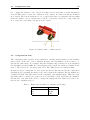
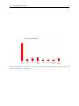
Autonomous System Lab
Semester Project
Obstacle detection
for the CRAB rover
Christophe Chautems
Prof. Roland Siegwart
Supervisors:
Ambroise Krebs
Cédric Pradalier
Januar, 2009
i
Abstract
To protect the CRAB rover, a mobile platform, obstacles need to be detected and avoided. It
is planned to fix a stereo camera on the rover and to use it to compute a map representing
the obstacle distribution, and send the map to the E* planner. The algorithm implemented is
based on the disparity image and is focused on the v-disparity. The project allowed to have
an overview of the capabilities of using the v-disparity and the limit of this technique. The
algorithm is implemented in C++ and is designed to be exported to the crab rover. The tests
on the algorithm show good results. Note that the obstacle detection is robust to variation in
camera position and partially to variations in camera orientation.
CONTENTS
ii
Contents
1 Introduction
1.1 Stereo vision . . . . . . . .
1.1.1 Stereo camera . . . .
1.1.2 Small Vision System
1.2 Content of the report . . . .
.
.
.
.
.
.
.
.
.
.
.
.
.
.
.
.
.
.
.
.
.
.
.
.
.
.
.
.
.
.
.
.
.
.
.
.
.
.
.
.
.
.
.
.
.
.
.
.
.
.
.
.
.
.
.
.
.
.
.
.
.
.
.
.
.
.
.
.
.
.
.
.
.
.
.
.
.
.
.
.
.
.
.
.
.
.
.
.
1
1
1
2
3
2 Methods
2.1 Camera position . . . . . . . . . . . . . . .
2.2 Coordinates Frames . . . . . . . . . . . . .
2.3 Strategy for obstacle detection . . . . . . .
2.3.1 First approach: Object segmentation
2.3.2 Second approach: Detection of floor
.
.
.
.
.
.
.
.
.
.
.
.
.
.
.
.
.
.
.
.
.
.
.
.
.
.
.
.
.
.
.
.
.
.
.
.
.
.
.
.
.
.
.
.
.
.
.
.
.
.
.
.
.
.
.
.
.
.
.
.
.
.
.
.
.
.
.
.
.
.
.
.
.
.
.
.
.
.
.
.
.
.
.
.
.
.
.
.
.
.
.
.
.
.
.
.
.
.
.
.
.
.
.
.
.
4
4
5
5
5
6
3 Implementation
3.1 Framework IPL . . . . . . .
3.2 Structure of implementation
3.3 Obstacle detection . . . . .
3.4 Driver . . . . . . . . . . . .
3.5 Image source . . . . . . . .
3.6 Disparity . . . . . . . . . .
3.7 V-disparity . . . . . . . . .
3.8 Floor detection . . . . . . .
3.9 Limit of obstacle . . . . . .
3.10 Display function . . . . . .
3.10.1 Show Line . . . . . .
3.10.2 Show obstacle . . . .
3.11 Map . . . . . . . . . . . . .
.
.
.
.
.
.
.
.
.
.
.
.
.
.
.
.
.
.
.
.
.
.
.
.
.
.
.
.
.
.
.
.
.
.
.
.
.
.
.
.
.
.
.
.
.
.
.
.
.
.
.
.
.
.
.
.
.
.
.
.
.
.
.
.
.
.
.
.
.
.
.
.
.
.
.
.
.
.
.
.
.
.
.
.
.
.
.
.
.
.
.
.
.
.
.
.
.
.
.
.
.
.
.
.
.
.
.
.
.
.
.
.
.
.
.
.
.
.
.
.
.
.
.
.
.
.
.
.
.
.
.
.
.
.
.
.
.
.
.
.
.
.
.
.
.
.
.
.
.
.
.
.
.
.
.
.
.
.
.
.
.
.
.
.
.
.
.
.
.
.
.
.
.
.
.
.
.
.
.
.
.
.
.
.
.
.
.
.
.
.
.
.
.
.
.
.
.
.
.
.
.
.
.
.
.
.
.
.
.
.
.
.
.
.
.
.
.
.
.
.
.
.
.
.
.
.
.
.
.
.
.
.
.
.
.
.
.
.
.
.
.
.
.
.
.
.
.
.
.
.
.
.
.
.
.
.
.
.
.
.
.
.
.
.
.
.
.
.
.
.
.
.
.
7
7
7
8
8
8
9
9
10
11
13
13
13
13
4 Results
4.1 Stability of the algorithm . . . . . . . . . . . . . . . . . . . . . . . . . . . . . . .
4.2 Computation time . . . . . . . . . . . . . . . . . . . . . . . . . . . . . . . . . . .
15
15
16
5 Discussion
5.1 Obstacles and floor tracking
5.2 Banking or not flat floor . .
5.3 Source image information .
5.4 Free space . . . . . . . . . .
18
18
18
18
19
.
.
.
.
.
.
.
.
.
.
.
.
.
.
.
.
.
.
.
.
.
.
.
.
.
.
.
.
.
.
.
.
.
.
.
.
.
.
.
.
.
.
.
.
.
.
.
.
.
.
.
.
.
.
.
.
.
.
.
.
.
.
.
.
.
.
.
.
.
.
.
.
.
.
.
.
.
.
.
.
.
.
.
.
.
.
.
.
.
.
.
.
.
.
.
.
.
.
.
.
.
.
.
.
.
.
.
.
.
.
.
.
.
.
.
.
.
.
.
.
.
.
.
.
.
.
.
.
.
.
.
.
.
.
.
.
.
.
.
.
.
.
.
.
.
.
.
.
.
.
.
.
.
.
.
.
.
.
.
.
.
.
.
.
.
.
.
.
.
.
.
.
.
.
.
.
.
.
.
.
.
.
.
.
.
.
.
.
.
.
.
.
.
.
.
.
.
.
.
.
.
.
.
.
.
.
.
.
.
.
.
.
.
.
.
.
.
.
.
.
.
.
.
.
.
.
.
.
.
.
.
.
.
.
.
.
.
.
.
.
.
.
.
.
.
.
.
.
.
.
.
.
.
.
.
.
.
.
.
.
.
.
.
.
.
.
.
.
.
6 Conclusions
20
References
21
List of Figures
22
List of Tables
23
A Content of CD
24
B Instruction to use obstacle detection
B.1 Small Visions System . . . . . . . . . . . . . . . . . . . . . . . . . . . . . . . . . .
25
25
CONTENTS
B.2 Obstacle detection . . . . . . . . . . . . . . . . . . . . . . . . . . . . . . . . . . .
B.3 Compile obstacle detection . . . . . . . . . . . . . . . . . . . . . . . . . . . . . .
C Configuration files
iii
25
25
26
1 Introduction
1
1
Introduction
To safely plan a path for a mobile robot from a starting to an end position, obstacles have to be
detected in order to be avoided. The goal of the project is to implement an obstacle detection
algorithm aiming at computing a map with the position of the obstacles. This work is dedicated
to the CRAB rover (figure 1) but the integration of the algorithm is out of its scope. The
passive structure of the CRAB rover adapts itself to the terrain shape and allows overcoming
small obstacles. This obstacle detection has to be usable to protect the rover against collision
therefores only the large obstacles have to be detected. This project is focused on the use of a
Stereo Camera and no other sensor is used.
Figure 1: CRAB rover, the stereo camera is not interfaced with the rover on the picture
1.1
Stereo vision
A stereo camera designed by the company Videre Design [8] is used in this work. The camera is
provided with software to acquire images, called Small Vision System (SVS). The two points of
view of a stereo camera allow to compute the distance to features on the image. This technique
refers to the binocular disparity which represents the different features location between the left
and right image. The construction of a disparity image is implemented in the software Small
Vision System and is not a part of this project.
An approach that has shown good result for an obstacle detection starting from a disparity
image is to compute the v-disparity and different groups worked on this [1][2][3]. The project
is focused on the v-disparity and allows having an overview of what can be achieved with this
technique.
1.1.1
Stereo camera
The model of the camera used is a STH-MDCS2-C (figure 2)[5]. The baseline, distance between
the two optics, is 9 cm and a focus lens of 6 mm is mounted on the camera. The lenses can be
changed to increase or decrease the focal length. The maximal resolution of the camera is 1280
1.1
Stereo vision
2
pixels horizontally by 960 pixels vertically, in this work, image with a maximal size of 640 by 480
are used. The reason is that the frame rate for image size 1280x960 is four time smaller than
for image size 640x480 (see table 1). The camera has to be connected through the firewire port.
This port carries power and commands from the computer and data block to it. A firewire hub
is set between the laptop and the camera because the laptop cannot supply the required current
to the camera.
Table 1: Frame rates in relation to resolution [5]
Resolution
1280x960
640x480
Frame rates
7.5 Hz
30 Hz
Figure 2: Stereo camera STH-MDCS2-C
1.1.2
Small Vision System
The Small Vision System (SVS) is provided by Videre Design and is implemented by the SRI’s
Artificial Intelligence Center [6] [9] [10]. It runs under Linux or Windows. SVS support image
acquisition, camera calibration, 3D reconstruction, and effective filtering. A calibration file can
be created by smallvcal [7] and this greatly improves the computed disparity. The coordinate
system for reconstructing 3D position is centered on the left camera’s focal point. The baseline
between the two optics is in the positive X direction. The coordinate system is displayed in
figure 3.
Figure 3: Stereo camera geometry with coordinate system centered on the left optic’s focal point
[6]
1.2
Content of the report
1.2
Content of the report
3
The next chapter presents the method used in this work. It describes what can be expected
from the obstacle detection and describes in which position and orientation the camera has to
be set. The coordinates frames used in this report are introduced. Two strategies for obstacle
detection are presented and evaluated.
The implementation of the algorithm is presented in the third chapter. First the framework use
and the structure of the implementation are presented, before to go in detail for each step of the
algorithm.
The results are presented in the fourth chapter where two points are described in detail. The
first one is the stability of the algorithm relative to change of camera orientation. The second
one is the computation time for each part of the algorithm.
The fifth chapter contains a discussion about some possible improvement of the algorithm. Those
improvements are presented with a first estimation of the time need to implement them. The
last chapter make a conclusion of the work on the project.
2 Methods
2
4
Methods
The ability to compute the distance based o n stereo image is studied before presenting the
algorithm.
The baseline and the focus define the resolution for the distance computation. Close to the
camera, there is a better resolution. The reason is that a change of one pixel in the ∆x image
feature represents a smaller distance. For that reason, there is a restriction on the upper distance
at which the robot can detect an obstacle. To detect an obstacle at five meters is not really
possible because the computation of its position is inaccurate. Furthermore, at such a distance
of five meters it is difficult to detect small obstacle and only the big one can be detected.
There is also a restriction on the lower distance. If the camera is looking too close, the field
of view (FOV) is smaller as the robot width. The consequence is that obstacles on the side of
the robot are not observable by the camera. In table 2 there is the field of view depending on
the focal lengths. The camera used in this work has a focus of 6 mm. Note thet other optics,
with different focus can be ordered and mounted on the camera. A change of focus can allow
observing obstacle closer or further to the robot.
Table 2: Horizontal and vertical field of view for different lens focal lengths [5]
Lens focal length
3.5 mm
6 mm
12 mm
16 mm
Horizontal FOV
87.1 deg
58.1 deg
31 deg
25.5 deg
Vertical FOV
71.1 deg
45.2 deg
23.5 deg
17.8 deg
A second restriction is that close to the stereo camera the disparity is important and it is difficult
to match a feature between the two images. The field of view is restricted because the pixels on
the side of the image do not have a corresponding pixel on the second image. For those reasons
the closest range for obstacle detection is around one meter.
2.1
Camera position
The camera position on the CRAB rover is at a height of 80 centimeters. The camera can
point in direction of the floor, there is no reason to observe the sky. The vertical field of view
of 45.2 deg is slightly reduced due to the mask size for the correlation between left and right
image. The disparity value cannot be computed for value on the border of the picture. The
angle θ (figure 4) between the direction of view and the horizontal has to be set in relation to
the distance at which the floor is observed. The formula in equation (1) gives the distance d in
front of the robot at which the floor can be observe in case of flat floor. F OVv is the vertical
field of view and h is the height of the camera.
d = tan(F OVv /2 · θ) · h
(1)
A good choice for the rotation angle θ of the camera is 15 deg. With this angle, the floor can
be observed at a minimal distance of one meter. As mentioned before for a shorter distance the
horizontal field of view is too small. With a rotation of 15 deg, the upper limit of the field of
view is about 5 deg above the horizontal. This part of the field of view can be useful in case that
2.2
Coordinates Frames
5
the slope is higher in front of the robot as in the robot position. That allows observing further
in this case.
2.2
Coordinates Frames
To estimate the distance and the height of an obstacle, the coordinate system of the camera has
to be transformed to a coordinate system with vertical and horizontal axis. The two coordinates
frames are illustrated in figure 4. In this purpose the camera coordinate frame can be rotated of
an angle θ around X-axis to have a coordinate system with the Z-axis representing the distance
to a point, the Y-axis the height and the X-axis the lateral distance. This second coordinate
frame is called the horizontal coordinate frame and denoted with h in the rest of this paper.
The transformation is expressed by a rotation matrix around the x axis. In equation (2) , there
is the transformation of a point from the camera coordinate frame to the horizontal coordinate
frame. With the transpose of the rotation matrix in equation (3), a point can be transformed
from camera coordinate frame to horizontal coordinate frame.
  
 
xc
1
0
0
xh
 yc  = 0 cos θ − sin θ  yh 
0 sin θ cos θ
zc
zh
(2)
 
  
xc
1
0
0
xh
 yh  = 0 cos θ sin θ   yc 
0 − sin θ cos θ
zh
zc
(3)
Figure 4: Coordinate frame
2.3
Strategy for obstacle detection
In a first step strategies to detect obstacles are developed and tested. For that purpose, some test
stereo images were taken in different environments. Seven pictures were taken in a parking lot
in the basement of a building and four outside. Those images are used to evaluate the strategies.
The test phase of the algorithms is done using Matlab. Two different strategies are tested and
presented in the next paragraphs.
2.3.1
First approach: Object segmentation
The first approach tested is to segment the image in different objects and then to check the
height and the slope of the objects. If the height or the slope are above a threshold, the object
2.3
Strategy for obstacle detection
6
is consider as an obstacle. This method shows good result for disparity image containing a small
amount of information. The reason is that in this case the object segmentation is easier to
implement.
The problem of this approach is that it depends on the objects segmentation. The task of
computing segmentation is difficult because the disparity images are imperfect. Depending of
the situation the segmentation can join two objects together or split one object in two that are
smaller as the threshold. For that reason, the development of this approach has been stopped
and a second strategy developed.
2.3.2
Second approach: Detection of floor
The second strategy detects the position of the floor and takes as obstacle every detected elements
above the floor using a threshold relative to the obstacle height. The disadvantage is that the
floor needs to be detected and mainly flat. The second assumption is not too restrictive if the
obstacles are observed in a distance range between 1m and 3m because on a small surface the
floor is often mainly flat.
This strategy is evaluated on the test images and shows good results. The floor is detected
on the eleven test images. This method is robust again change of parameter for the stereo
computation such as filter parameters. The result for the test image depicted on figure 5(a) is
shown in figure 5(b). The field of view is represented by the two blue lines on the map and the
left camera focal point is at position X = 0 and Y = 0. The implementation of this method is
described in detail in the next chapter.
(a) Left test image
(b) Map of the test image
Figure 5: Result of the second approach: Detection of floor
3 Implementation
3
7
Implementation
The algorithm is implemented in C++ and uses the framework IPL implemented by Cédric
Pradalier. The advantage of this framework is that the management of the memory is already
implemented and use Dynamic Data eXchange (DDX) [4]. DDX allows a coalition of programs
to share data at run-time through an efficient shared memory mechanism. The image processing
and the image display are divided in two executables. The image processing is done by IPLObstacleDetection and the display is done by sdlprobe. The two executables access to the same
object in the memory. The access is controlled by DDX. In case the display is not needed, only
the processing part can be executed. An instruction to run the program IPLObstacleDetection
is available in appendix B.
The image processing is controlled by a processing tree defined in a driver. The implementation
of the IPL framework is defensive and this help to avoid some error in the program. The inputs
are checked to be correct before being processed. The framework also compute the time for each
of the processing step, that allows seeing which part of the algorithm needs to be improved to
increase the computation speed.
The libraries provide by Videre Design for the video acquisition and the disparity computation
had to be integrated in the framework.
3.1
Framework IPL
The structure of the image processing algorithm is implemented in the class ”IPLDriver”. In the
driver, there is a successions of operation performed on the image. Each operation is executed by
an object that inherits from the generic parent class ”IPLImageProcessor”. The main processing
class is divided in different subclasses depending on the operation to perform. The subclasses
used in this project are the following:
• IPLImageSource: has no input image and output a set of images
• IPLImageFilter: has one input object and output has many images has in the input
• IPLBinaryOperator: has two inputs objects and one output object
In each of this class, a function checks if the inputs have the correct format. Then, if the inputs
are correct, another processes those in order to achieve the right operation.
3.2
Structure of implementation
The algorithm is split in different blocks. Each one of the blocks is a class that inherits from the
class ”IPLImageProcessor”. On the figure 6, there is a diagram with all the classes implemented
during the project. There are also some classes that are used to display what the algorithm does
and for debugging purpose. All the blocks for the display can be suppressed because they are
not needed to compute the map.
The executable reads a configuration file with parameters for the disparity computation and the
obstacle detection. This configuration file makes easier to change some parameters such as the
obstacle’s height. An exemple of configuration file is vdisp.cfg in appendix C. The goal is to send
to the E* planner the map, this part of the information processing is not implemented.
3.3
Obstacle detection
8
Figure 6: Structure of implementation of the obstacle detection algorithm
3.3
Obstacle detection
The main function of the program ObstacleDetection begin with the construction of objects of
the class svsVideoImages and svsStereoProcess. Those two classes are supplied with the SVS
software and support the images acquisition and the stereo processing. The construction of the
driver and the building of the processing tree are done in the main function. The driver is called
in the main function. When the program exits, the stopping and closing of the svsVideoImage
object are done in the main function.
3.4
Driver
The driver is the part of the program that controls the data flow of the algorithm all the different
blocks are called by the driver. The structure presented in the previous chapter is implemented
in the driver called IPLObstacleDetectionDriver.
3.5
Image source
The image source block uses the function given by the company Videre Design. It manages the
images acquisition, and the images rectification. The path of the calibration files has to be set in
the configuration file. This configuration file is created by the software smallvcal. Information
about the calibration procedure can be found in Small Vision System Calibration Supplement
to the User’s Manual Software [7].
The computation of the disparity image takes also place in this class. In the configuration file
parameters for the disparity computation and for the filters implemented in SVS can be set. In
table 3, there is an overview of those parameters. Detailed explanation can be found in the
Small Vision System User’s Manual Software on chapter 2.4.4, 2.4.7 and 2.5 [6].
3.6
Disparity
9
Table 3: Disparity parameter in configuration file vdisp.cfg
Name
ndisp
coorsize
thresh
unique
SpeckleSize
SpeckleDiff
Description
Disparity search range
Correlation window size
Confidence filter threshold
Uniqueness threshold
Smallest area that is considered as valid disparity region
Maximum difference between neighboring disparity pixels
(a) Left image (640x480)
Units
[pixel]
[pixel]
[-]
[-]
[pixel]
[1/4 of a pixel]
(b) Disparity image (640x480)
Figure 7: Left image and resulting disparity image
3.6
Disparity
As mentioned before the disparity is computed in the image source block by the svsStereoProcess.
The values for the disparity are saved in an array of the type short. An important parameter for
the disparity computation is the disparity search range. This parameter defines the range in with
a matching between the left and the right image is searched. The variable for this parameter
is called ndisp in the configuration file and the unit is in pixel. For example if the value is set
to 48, the algorithm searches match between the left and the right image until a distance of 48
pixels. The disparity is represented in 1/16 of a pixel. It means that a value of 16 in disparity
image represents a distance of one pixel between the left and right image. The pixels that are
rejected by the filter implemented in SVS have a negative value on the disparity image.
The disparity image needs only to be copied in the framework. The disparity image from the left
and right stereo image is depicted in figure 7(b). All the important edges from the left image on
figure 7(a) are on the disparity image. The elements close to the camera have high values and
are bright on the disparity image. Inversely those far from the camera have a small disparity
and are dark.
3.7
V-disparity
The v-disparity is computed from the disparity image. Each line of the disparity image corresponds to the same line on the v-disparity. The column on the v-disparity corresponding to the
value read on the disparity is increment by one. The height of the v-disparity is the same as
the disparity image and the width is equal to the maximum value in the disparity image. In
figure 8 the v-disparity from the disparity image in figure 7(a) is shown. The points on the left
3.8
Floor detection
10
of the image have a small disparity and are far from camera. The points on the right are close
to camera.
The advantage is that the floor is mapped on a line. On the disparity image (figure 7(b)) the
floor is represented by a color shading. The floor in the lower part of the image is close to the
camera. In the upper part of the image, the floor is far from camera. The color shading between
the lower part and the upper part of the image is matched as a line on the v-disparity. An
obstacle in front of the camera is represented by a uniform color on the disparity because all the
points are at the same distance. This obstacle with uniform color is matched as a vertical line
on the v-disparity.
Figure 8: V-disparity image (768x480)
Input: disp(width, height) ← Disparity image
Output: vdisp(maxdisp, height) ← V-disparity image
foreach ith column on disp do
foreach j th line on disp do
if disp(i,j) > 0 then
vdisp(disp(i,j),j) ++
end
end
end
Algorithm 1: The v-disparity algorithm
3.8
Floor detection
The floor detection is done with a Ransac (Random Sample Consensus). A vector of points
is constructed with all the pixels with higher value than a threshold on the v-disparity. The
threshold is currently set to three to reject pixels with low value on the v-disparity. Two points
are randomly chosen and used to construct a line. The slope of the line is checked to be in the
right range for the floor and if it is the case the points close to the line are counted. This step is
iterated and the line with the bigger amount of point close to it is kept as the line representing
the floor. This line is represented by an array. Each element represents one column on the vdisparity and the value of the element represents the position of the line. The line can be ploted
on the disparity with the IPLShowLine class. The results of the display function is available in
figure 9.
If the position of the line is smaller than zero or bigger than the image height, the value is set
to zero. Some parameters for the floor detection can be set in the configuration file. Those
parameters are listed in the table 4.
3.9
Limit of obstacle
11
Table 4: Floor detection parameters in configuration file vdisp.cfg
Name
minRansac
iterRansac
anglefloorMin
anglefloorMax
distThres
Description
Minimum number of selected pixel to applied RANSAC
Number of iteration of RANSAC
Minimal angle between horizontal and floor’s line
Maximal angle between horizontal and floor’s line
Threshold to count a point as close to the line
Units
[pixel]
[-]
[rad]
[rad]
[pixel]
Input: vdisp(maxdisp, height) ← V-disparity image
Output: f loor(maxdisp, 1) ← Line representing the floor
foreach ith column on vdisp do
foreach j th line on vdisp do
if vdisp(i,j) > 3 then
listpoints ← Add (i, j) to list of points
end
end
end
if No. of points in listpoints >minRansac then
no pointbest ← 0;
for 1 to iterRansac do
Select randomly two points in listpoints;
(a, b, c) ←Compute the equation a · x + b · y + c = 0;
angle ← arctan((−a)/b);
if (angle<anglefloorMax) & (angle>anglefloorMin) then
no point ← 0;
foreach nth point in listpoints do
dist ← distance from nth point to line;
if dist<distThres then
no point + +;
if no point>no pointbest then
bestLine ←Parameter of line;
end
end
end
end
end
end
foreach k th column of floor do
f loor(k, 0) ← Position of bestLine in k th column ;
end
Algorithm 2: Floor detection
3.9
Limit of obstacle
To define the minimal size which corresponds to an obstacle, the algorithm takes a line above the
floor relative to the obstacle height. This is done by checking the vertical distance between two
points on the v-disparity. The first point above the line representing the floor with a distance
bigger as the minimal obstacle height is marked as the limit of obstacle. The angle between
3.9
Limit of obstacle
12
Figure 9: Line representing the floor plot on v-disparity image
the direction of view of the camera and the horizontal can be set in the configuration file. This
angle is needed to transform a 3D point from the camera coordinate to a coordinate frame
with a vertical axis. A second parameter than can be set is the obstacle height. The line is
represented like the floor by an array. In the figure 10, the line representing the floor and the line
representing the limit of obstacle are displayed. On the left side of the image the two lines come
close, because a pixel difference represents a bigger distance for points far from camera.
Figure 10: The lower line represents the floor and upper line the limit line of obstacle
Input: f loor(maxdisp, 1) ← Line representing the floor
Output: limit(maxdisp, 1) ← Line representing limit of obstacle
foreach ith column of floor do
(Xcf , Ycf , Zcf ) ← Compute 3D coordinate of floor;
(Xhf , Yhf , Zhf ) ← Transform (Xcf , Ycf , Zcf ) to horizontal coordinate frame ;
foreach j th point above the floor do
(Xcj , Ycj , Zcj ) Compute 3D coordinate of j th point;
(Xhj , Yhj , Zhj ) ← Transform (Xcj , Ycj , Zcj ) to horizontal coordinate frame ;
verticaldist ← |Zhj − Zhf |;
if verticaldist>obstacleheight then
limit(i, 0) = j;
break;
end
end
end
Algorithm 3: Limit of obstacle
3.10
Display function
3.10
Display function
13
The display functions are not needed by the algorithm to process the map and are mainly used
to understand how the algorithm works and for debuging purpose.
3.10.1
Show Line
It plots a line on a v-disparity image. The line representing the floor on the v-disparity can
be seen in the figure 9. This class can also be used to plot the limit of obstacle on the vdisparity.
3.10.2
Show obstacle
There is also one block for the display of the obstacles. It displays the points from the disparity
that are considered as obstacles. For each pixel in the disparity image, it checks if the pixel is
above the limit corresponding to the obstacle’s line. If the pixel is above the line, it is set to one
on the image and else to zero. The size of the image is the same as the disparity. The pixels
with value equal to one are the obstacles. The result can be observed in figure 11. All the pixels
representing the floor on the disparity in figure 7(b) are not detected as obstacle.
Figure 11: Pixels on the disparity image that are detected as obstacle
3.11
Map
All the points that are above the limit corresponding to the obstacle’s line is projected on a 2D
discrete map. To select the points, the same method is used as to show obstacles. For each pixel
in the disparity image it checks, if the pixel is above the limit corresponding to the obstacle’s
line. In case that the pixel is above the line, the 3D coordinates of the point in the camera
coordinate frame are transformed to give the horizontal distance to the camera. The square on
the 2D map corresponding to this point is increment by one.
The map has a resolution of 10cm in both directions. The size of the map is 5m by 5.1m. The
reason for this limitation is that at longer distance the position of an obstacle is not accurate. The
position of the left camera focal point is at the center on the bottom of the map. A transformation
to a coordinate frame with an horizontal axis is needed to compute the horizontal distance to
an object. The angle of the camera can be set in the configuration file. In figure 12, there is the
resulting map of the previous images.
3.11
Map
14
Figure 12: Map of obstacles, the red point is the camera position, the blue line is the limit of
the field of view
The values in a square of the map corresponds to the number of pixels that are mapped on this
square. Small obstacles have low values on the map because they have few pixels representing
them and big obstacles have high value. The obstacles close to the camera have higher values as
the obstacles far from camera. The reason is that obstacles close are bigger on the image, and
have more pixels to represent them. This is useful as it means the obstacle detection performs
better at close range. The computation of the obstacle’s position is more accurate for close
obstacles. The value on the map is in relation to the probability of an obstacle and the size of
the obstacle. The only limit on the maximal value is the maximal value that can be store in a
short signed integer. The maximal value store by a short signed integer is 32,767.
Input: limit(maxdisp, 1) ← Line representing limit of obstacle
Input: disp(width, height) ← Disparity image
Output: map(51, 50) ← 2D discrete map
foreach ith column on disp do
foreach j th line on disp do
if disp(i,j)>0 then
if line((disp(i,j)),0)>j then
(Xc , Yc , Zc ) ← Compute the 3D coordinate in camera coordinate frame;
(Xh , Yh , Zh ) ← Transform (Xc , Yc , Zc ) to horizontal coordinate frame ;
if Xh < 5 then
(Xpos , Ypos , Zpos ) ← f loor((Xh , Yh , Zh ) · 10);
map(25 + Ypos , 50 − Xpos ) + +
end
end
end
end
end
Algorithm 4: Map
4 Results
4
15
Results
The algorithm shows good result, each of the obstacles on the disparity image are projected on
the map. The five obstacles on figure 13(a) that have enough texture to compute the disparity
(figure 13(b)) are projected on the map (figure 14). The problem of this indoor environment
is that due to the lack of texture only the edges of the objects are detected. On a uniform
background the disparity algorithm cannot match a feature from the left image on the right
image. With an outdoor environment, there is more texture and more information on the
disparity image.
(a) Left image
(b) Disparity image
Figure 13: Left image and resulting disparity image, with five objects marked on both image
Figure 14: Map of obstacles
4.1
Stability of the algorithm
The algorithm stability is described in relation to a modification of the camera position or
orientation. If the height of the camera is changed the algorithm continues processing well.
There is no problem to detect the floor and to estimate the distance to an obstacle. In case of
variation in the orientation of the camera it depends around with axis the camera rotates, the
axis that are used to describe the stability are the same as on the figure 15. A rotation around
the Y-axis is armless and the map is correctly computed with the new orientation of the camera.
With a rotation around the X-axis, the algorithm is still able to detect the floor but the problem
4.2
Computation time
16
is to compute the distance to the obstacle. For that reason it is useful to read the information
from the IMU sensor to know the orientation of the camera. A rotation around the Z-Axis is
more critical. The reason is that the floor does appear has a line on v-disparity. The algorithm
shows the ability to detect a mean value for the floor but if the rotation is too important, the
floor on the side of the image can appear as an obstacle.
Figure 15: Camera with coordinate system
4.2
Computation time
The computation time depends on the parameters. An important parameter is the disparity
range search. If the size of the v-disparity increases, the algorithm needs more time to go
through the entire image. For example when the disparity range search is set at 48 disparities
the algorithm can run at 10Hz. For other disparity range search, the result are available in the
table 5. The test is done on a laptop with a Core Duo 2Ghz Prossecesor with 1Go Ram.
In figure 16, the processing time for each operation is shown. The time used for the computation
is mainly used for acquiring the images source and computed the disparity. The algorithm is not
optimized but half of the time is used for the computing of the disparity image. This part of the
algorithm cannot be improved because it is done externally by SVS and is already optimized.
Around 20% of the time is also used to compute the display windows. This can be removed to
increase the computation speed.
Table 5: Frame rates in relation to disparity search range.
Number of disparity
32
48
64
Frame rates
15 Hz
10 Hz
6 Hz
4.2
Computation time
17
Figure 16: Computation time for each block, with disparity computation in image source, disparity search range of 48 disparities
5 Discussion
5
18
Discussion
In this chapter, different improvements of the algorithm are presented and discussed. A first
estimation of the different improvements and their result is presented.
5.1
Obstacles and floor tracking
The algorithm only makes an instantaneous map of the environment and do not take into
account the information from the previous iteration. The information of the previous iteration
can be used in different ways to improve the algorithm. A first idea is to search the floor in
a smaller interval close to the previous floor. That will restrict the search space and improve
the computation speed. The speed increase will stay small because only a few amount of the
computation time is used for approximate the floor. The second idea is to keep the position of
the obstacles in memory and joins the map extract from different iterations. This will not really
improve the algorithm if the robot is not moving. But if the robot moves, the points of view
changes between the different iteration and the information on each map will be different. To
regroup the information of the maps, the position of the robot has to be known. This part of
the algorithm can only be applied if the odometry of the mobile robot is known.
5.2
Banking or not flat floor
The implementation shows the ability to detect obstacles. But there is some restriction concerning the flat floor in front of the robot. The algorithm is not able to detect a banking floor, the
slope of the floor can only be in the moving direction of the robot. An improvement could be
achieved by approximating the plan of the floor with the 3D point and not using the v-disparity.
That avoids the problem that a banking floor is not represented by a line on the v-disparity.
This extension can be implemented in a couple of day. The search space is bigger because
three parameters are needed to define the floor. In comparison, the v-disparity only needs two
parameters.
As second possible improvement is to split the image in part and then detect for each part a
local floor. That allows approximating a not flat floor. The problem is that each image part
has less information to approximate the floor and it can be difficult to found the floor for each
of the part.
5.3
Source image information
To improve the detection of homogenous objects, segmentation can be applied on the image
source. The disparity can be computed for the edge of homogenous surfaces. Starting from
the edge, the distance for the entire surface can be determined. This approach is more difficult
to implement because information coming from disparity and image source are to be combined
together. A lot of different cases can appear and it can be really long to develop an algorithm
working in each case. But this cue is use by the human vision and implementing it in robot
vision can improve the obstacle detection.
5.4
Free space
5.4
Free space
19
In the algorithm, only the obstacles are detected but it can be useful to detect the free space.
The free space means the space where there is no obstacle. The free space is the place where
the floor can be seen. It is all the points close to the floor line on the v-disparity. Create a map
with the free space is easy to implement. The point that has still to be studied is how to join
together the free space map and the obstacle map.
6 Conclusions
6
20
Conclusions
In this work, an algorithm was implemented to generate an obstacle map, based on the stereo
camera data. The algorithm showed good result and run at 10 Hz. The algorithm is robust to
variation in camera position and partially to variations in camera orientation. The implementation is focused on the v-disparity and allows acquiring a lot of information about what can
be done with the v-disparity. The algorithm detects the floor on the v-disparity. An object is
considered as an obstacle if it is above the floor.
The algorithm shows good result and stability. Two possible causes of failure are identified. The
first is a lack of texture. In most of the outdoor environment, there is a lot of texture and the
CRAB rover is designed to be use outdoor. The second cause of failure is a banking floor but if
the obstacles are detected on a short distance, this problem can be overcome.
Due to the stability of the algorithm, the conclusion is that the algorithm can be exported
to the CRAB rover to continue the tests and confirm the results in a real environment. The
improvement on the algorithm that has priority is to interact with the odometry of the CRAB
rover in the goal of tracking the obstacles. Two other improvements which can probably show
good results are to mark the free space and to approximate the floor with 3D points to deal with
a banking floor.
REFERENCES
21
References
[1] A. Broggi, C. Caraffi, R.I. and Fedriga, and P. Grisleri : Obstacle Detection with Stereo
Vision for Off-Road Vehicle Navigation, Procs. Intl. IEEE Wks. on Machine Vision for
Intelligent Vehicles, 2005
[2] C. Caraffi, S Cattani, and P. Grisleri : Off-Road Path and Obstacle Detection Using Decision
Networks and Stereo Vision, IEEE Transactions on intelligent transportation systems, vol.8
No.4, December 2007
[3] R. Labayrade, D. Gruyer, C. Royere, M. Perrollaz, and D. Aubert: Obstacle Detection
Based on Fusion Between Stereovision and 2D Laser Scanner, Mobile Robots: Perception
& Navigation, Book edited by: Sascha Kolski, ISBN 3-86611-283-1, pp. 704, February 2007
[4] P. Corke, P. Sikka, J. Roberts, and E. Duff: DDX: A Distributed Software Architecture
for Robotic Systems, Proc. of the Australian Conf. on Robotics and Automation, Canberra
(AU), December 2004
Technical Documentation
[5] Videre Design: STH-MDCS2/-C Stereo Head User’s Manual, 2004
[6] SRI International Small Vision System User’s Manual Software version 4.4d, May 2007
[7] SRI International Small Vision System Calibration Supplement to the User’s Manual Software version 4.4d, May 2007
Internet Links
[8] Videre Design http://www.videredesign.com/
[9] SRI International http://www.sri.com/
[10] SRI Stereo Engine http://www.ai.sri.com/ konolige/svs/index.htm
LIST OF FIGURES
22
List of Figures
1
2
3
4
5
6
7
8
9
10
11
12
13
14
15
16
CRAB rover, the stereo camera is not interfaced with the rover on the picture . .
Stereo camera STH-MDCS2-C . . . . . . . . . . . . . . . . . . . . . . . . . . . .
Stereo camera geometry with coordinate system centered on the left optic’s focal
point [6] . . . . . . . . . . . . . . . . . . . . . . . . . . . . . . . . . . . . . . . .
Coordinate frame . . . . . . . . . . . . . . . . . . . . . . . . . . . . . . . . . . . .
Result of the second approach: Detection of floor . . . . . . . . . . . . . . . . . .
Structure of implementation of the obstacle detection algorithm . . . . . . . . . .
Left image and resulting disparity image . . . . . . . . . . . . . . . . . . . . . . .
V-disparity image (768x480) . . . . . . . . . . . . . . . . . . . . . . . . . . . . . .
Line representing the floor plot on v-disparity image . . . . . . . . . . . . . . . .
The lower line represents the floor and upper line the limit line of obstacle . . . .
Pixels on the disparity image that are detected as obstacle . . . . . . . . . . . . .
Map of obstacles, the red point is the camera position, the blue line is the limit
of the field of view . . . . . . . . . . . . . . . . . . . . . . . . . . . . . . . . . . .
Left image and resulting disparity image, with five objects marked on both image
Map of obstacles . . . . . . . . . . . . . . . . . . . . . . . . . . . . . . . . . . . .
Camera with coordinate system . . . . . . . . . . . . . . . . . . . . . . . . . . . .
Computation time for each block, with disparity computation in image source,
disparity search range of 48 disparities . . . . . . . . . . . . . . . . . . . . . . . .
1
2
2
5
6
8
9
10
12
12
13
14
15
15
16
17
LIST OF TABLES
23
List of Tables
1
2
3
4
5
6
Frame rates in relation to resolution [5] . . . . . . . . . . . . . . . . .
Horizontal and vertical field of view for different lens focal lengths [5] .
Disparity parameter in configuration file vdisp.cfg . . . . . . . . . . . .
Floor detection parameters in configuration file vdisp.cfg . . . . . . . .
Frame rates in relation to disparity search range. . . . . . . . . . . . .
Default and supported value for parameters in configuration file . . . .
.
.
.
.
.
.
.
.
.
.
.
.
.
.
.
.
.
.
.
.
.
.
.
.
.
.
.
.
.
.
.
.
.
.
.
.
2
4
9
11
16
27
A Content of CD
A
24
Content of CD
The CD contains the following folders:
• svs44g: Small Vision System 4.4g, Sales Order with password to connect to Videre Design
website
– ManualStereoCamera: manual for SVS and for camera STH-MDCS2
• IPipeLine: IPL Framework
– SDL: executable sdlprobe for display
– IPL: IPL source file
– ObstacleDetection: Implementation of obstacle detection
∗ Calibration: Calibration file created with smallvcal
∗ svs: Library and source from Small Vision System
• Test Stereo Image: Test stereo images
– Parking: Seven images taken in parking lot
– Garage: Four images taken outside
• Presentation: Mid-Term and Final Presentation
• OD Report: Latex source
B Instruction to use obstacle detection
B
25
Instruction to use obstacle detection
B.1
Small Visions System
Run SVS:
1. Extract the files from svs44g.tgz
2. Follow the instruction from the manual (Small Vision System User’s Manual Software
version 4.4d) in file smallv-4.4d.pdf.
B.2
Obstacle detection
To use the obstacle detection on the CD in the directory IPipeLine, the Intel Integrated Performance Primitives(IPP) and the Dynamic Data eXchange (DDX) are need.
1. Before Starting IPLObstacleDetection allocate memory with:
catalog &
store -m 32m &
if no internet connection also use:
sudo route add -net 224.0.0.0 netmask 240.0.0.0 dev eth0
otherwise it blocks DDX
2. Set the path for the camera calibration file in vdisp.cfg
3. Run in folder IPipeLine/Vdisparity: ./IPLObstacleDetection vdisp.cfg and let it runs.
4. For display run in parallel in folder IPipeLine/SDL: ./sdlprobe IPLObstacleDetection
To see the different display of the processing tree use the arrows on the keyboard.
B.3
Compile obstacle detection
1. To change makefile, edit CMakeLists.txt in the directory IPipeLine/ObstacleDetection
and then run cmake . in the directory IPipeLine.
2. Run make in the directory IPipeLine/ObstacleDetection
C Configuration files
C
26
Configuration files
In this appendix, there is a configuration file with default value that shows good result. This
file can be found on the CD under the name vdisp.cfg,
[main]
middleware = "ddx"
period = 0
debug = 1
[image source]
width=640
height=480
ndisp=48
corrsize=11
thresh=10
unique=10
SpeckleSize=100
SpeckleDiff=4
paramfile="/home/chautemc/Project/IPipeline/ObstacleDetection/Calibration/calibration.ini"
[Floor]
minRansac=100
iterRansac=100
anglefloorMin=0.1
anglefloorMax=0.9
distThres=4
[Limit obstacle]
max_height=0.20
angRot=0.26
[Map]
angRot=0.26
Name
middleware
period
debug
width
height
ndisp
coorsize
thresh
unique
SpeckleSize
SpeckleDiff
paramfile
minRansac
iterRansac
anglefloorMin
anglefloorMax
distThres
max height
angRot
100
100
0.1
0.9
4
0.2
0.26
Default
”ddx”
0
1
640
480
48
11
10
10
100
4
Table 6: Default and supported value for parameters in configuration file
Supported values
Description
never tested
Middleware used
never tested
To define image processing period
never tested
Print messages
support only this value Source image width
support only this value Source image height
16,32,48,64
Disparity search range
9,11,13
Correlation window size
0-15
Confidence filter threshold
0-10
Uniqueness threshold
0-100
Smallest area that is considered as valid disparity region
never tested
Maximum difference between neighboring disparity pixels
Path for calibration file
2-1000
Minimum number of selected pixel to applied RANSAC
10-200
Number of iteration of RANSAC
0-1.5
Minimal angle between horizontal and floor’s line
0-1.5
Maximal angle between horizontal and floor’s line
1-10
Threshold to count a point as close to the line
0.1-0.5
Maximal height of obstacle
0.1-0.4
Angle between camera and horizontal
Units
[-]
[-]
[-]
[pixel]
[pixel]
[pixel]
[pixel]
[-]
[-]
[pixel]
[1/4 of a pixel]
[-]
[pixel]
[-]
[rad]
[rad]
[pixel]
[m]
[rad]
C Configuration files
27