1
PC Oscilloscope
Spectrum Analyzer
Logic Analyzer
DSO-50x12 Series
User’s Manual
Revision I
http://www.clock-link.com.tw
Accessories Contents .................................................................................. 2
System Requirements ................................................................................. 2
Installing Hardware ...................................................................................... 2
Installing Software ....................................................................................... 2
Feature ........................................................................................................ 3
Guide to Operations .................................................................................... 3
Main Screen ................................................................................................ 4
Horizontal Scroll Bar .................................................................................... 4
Vertical Scroll Bar ........................................................................................ 5
Hardware Specifications .............................................................................. 5
DSO-50212 Hardware Specifications ..............................................................................5
DSO-50412 Hardware Specifications ..............................................................................6
Hot Keys Function ....................................................................................... 7
Tool Bar ....................................................................................................... 8
File Menu..................................................................................................... 9
View Menu ................................................................................................. 10
Setup Menu ................................................................................................11
Logic Menu ................................................................................................ 12
Channel Box .............................................................................................. 15
Trigger Box ................................................................................................ 18
Measurements ........................................................................................... 22
Parameter Measurements ......................................................................... 22
FFT ............................................................................................................ 23
State List.................................................................................................... 24
USB driver install ....................................................................................... 25
Windows 2000 USB driver install................................................................................... 25
Windows XP USB driver install ...................................................................................... 28
Windows Vista USB driver install................................................................................... 30
Technical Support ...................................................................................... 33
Software Updates ...................................................................................... 33
APPENDIX ................................................................................................ 34
Fast Fourier Transformations..................................................................... 34
Understanding FFT’s Application............................................................... 34
Typical FFT of Applications........................................................................ 34
Fundamental Principles ............................................................................. 34
Magnitude.................................................................................................. 35
Decibel (db) ............................................................................................... 35
Logarithm................................................................................................... 35
The Characteristics of Weight Function..................................................... 36
Functionality .............................................................................................. 36
FFT ................................................................................................................................ 37
Bw.Sweep...................................................................................................................... 37
Source ........................................................................................................................... 37
Points............................................................................................................................. 37
Window.......................................................................................................................... 37
Gain Type ...................................................................................................................... 37
1
Accessories Contents
• The DSO-50x12 Series Aluminum unit.
• Logic Analyzer Pod.
• Two pieces (DSO-50212) or Four pieces (DSO-50412).
calibrated 300MHz Probe with (x1, x10). 10pF input Capacitance.
• Housing with twenty piece color wires and easy hook clips.
• USB 2.0 cable.
• Universal Power Supply with DC Adapter 12V/1A (DSO-50212), 12V/2A (DSO-50412). .
• DSO-50x12 Series User's Manual.
• Control Software CD.
System Requirements
In order to use the DSO50x12, the following equipment is necessary:
• Computer System:
Pentium PC system with at least one USB interface
(USB 1.1 or 2.0 version).
• Memory: A minimum of 256 MB free RAM. 512 MB or 1GB is better.
• Mass Storage: At least one CD drives and hard disk drives.
• Monitor: Any monitor compatible with the above display adapter.
• Operation System: Windows 2000/XP/VISTA.
Installing Hardware
• Connects USB cable to DSO.
• Setup USB driver from CD.
• Plug in power source from +12V DC Adapter.
• Waiting for control software turn on.
Installing Software
• Insert the distribution CD into drive E: (here E: is CD driver).
• Enter file to run E:\DSO50x12\dso50x12.exe.
• Follow the on screen instructions.
2
Feature
• Innovative cross triggering: logic analyzer channels can trigger the analog channels and
vice versa.
• Long time pre-triggering up to 262143*256 points, about -67M points.
• Fast data capture and screen update rates.
• Hot key function that is convenient to use.
• Deep 512K/2M sample data acquisition buffers on each channel (A1, A2, A3, A4, D0 ~ D11).
• Precision 200MHz Frequency counter, up to 7 digital resolution @ 512K memory for each
analog channel.
• Advance Fast Fourier Transformations function to Bandwidth test.
• Support Pulse width and TV(NTSC525, PAL625) Triggering and count.
• Support high speed (up to 50MHz SCL clock) I²C , SPI Triggering.
• Support I²C, SPI, UART, more... serial bus timing encode.
• Convenient Timing state display for logic debug.
Guide to Operations
When making measurements with the Digital Storage Oscilloscope / Logic Analyzer Cards,
meaningful data can only be captured with some prior knowledge of the characteristics of
the circuit under test.
Before initiating any capture cycles, the DSO must be configured using the control program.
See the software section later in the manual for instructions on these procedures.
To connect the DSO to the test circuit, there are two standard BNC probes, one for each
Analog input channel, and a series of mini-clips on the Logic Analyzer Pod for the Logic
Input channels. The scope probes have removable hook clips on their ends and an attached
alligator clip for the signal ground connection. The Logic Analyzer Pod has inputs for 12
channels, D0 channel is the external clock input, and 8 ground points.
For synchronous data captures, external clock sources can be connected to the D0 channel.
At times, it may also be necessary to connect the test circuit to the computer system itself.
This will eliminate more noise in the test application due to ground level differentials. This is
especially true when dealing with high speed timing analysis. Use a heavy gauge wire to
make a connection between the test circuit ground and the case of the computer.
Each Analog channel probe has a calibration adjustment. It is important that this calibration
be made at least twice a year. See Calibration for more information.
When connecting the probes to any signal, make sure that the signal voltage is
Within the limits of the DSO. check the technical information section for absolute
maximum and recommended maximum input voltages for the probes.
Logic Analyzer Pod Markings:
D0 ~ D11 Channel data inputs.
GND Signal ground connection.
3
Main Screen
Horizontal Scroll Bar
This scroll bar is used in conjunction with a selected waveform or cursor. The Horizontal Scroll
Bar will move a selected waveform or cursor left or right in the display area.
The Horizontal Scroll Bar works with Display, Analog input channels, Memory, Logic Analyzer
channels, V1Bar, V2Bar, and Trigger Bar.
4
Vertical Scroll Bar
This scroll bar is used in conjunction with a selected waveform or cursor.
The Vertical Scroll Bar will move a selected waveform or cursor up or down in the display area.
The Vertical Scroll Bar works with Display, Analog input channels, Memory, H1Bar, and H2Bar.
Hardware Specifications
DSO-50212 Hardware Specifications
Model
Record Length
Sampling Rate
External clock
Timebase Accuracy
Analog Channel
Input Bandwidth
Input Impedance
Max. input voltage
Input Sensitivity
Vertical Accuracy
Trigger Sensitivity
Trigger Level
Trigger Type
Digital Channel
Input Bandwidth
Input Impedance
Input Sensitivity
Channel skew
Max. Input Voltage
Threshold Voltage
Trigger Qualify
Operate
Power Supply
Power consumption
PC Interface
Net Weight
Size (Dimension)
Accessories
DSO-50212
2MB / Ch
Ch.A1: 1Sa/s to 1Gsa/s
Ch.A2: 1Sa/s to 500MSa/s
D0 ~ D11:1Sa/s to 500MSa/s
1KHz to 50MHz (max.)
50ppm
Ch.A1, Ch.A2
ChA1: 200MHz (3db)
Ch.A2:100MHz (0.5db), 125MHz (1db)
1Mohm // 15pF
50v (100v Transient)
5mv/div to 2v/div
+/- 1.5%
0.2 div (250MHz)
Adjustable 250 level
Slope +/-, Pulse width +/-, TV (NTSC / PAL),
Horizontal Synchronous Count Trigger.
D0 ~ D11 (12ch)
150MHz (max.)
100K ohm || 2pF
< 500mv
< 2ns
+/- 50v (100v Transient)
-2v to +6v
Parallel: 0, 1, X (don't care) settings for all
Digital channels
I²C: 0, 1, X (don't care) settings for 4 (bytes+
Ack) long
SPI: 0, 1, X (don't care) settings for 36bit long
Mouse
DC Adapter 12V/1A
USB +5V: <250mA+12V: <500mA
USB (Version 1.1/2.0)
1.2 KGS
220mm x142mm x 40mm
Logic Analyzer pod, USB 2.0 cable.
Calibrated Probe 300MHz (1:1, 10:1) x 2 pcs.
User's Manual, Software CD.
Housing with Color wires & clips x 16 pcs.
DC Adapter 12V/1.0A.
5
Remark
Points
Realtime: from 10Sa/s to
1GSa/s.
Software catch: from 1Sa/s
to 200Sa/s.
From Logic Channel D0
8bit resolution
@BNC connect (Probe 10:1)
@BNC connect (Probe 1:1)
10 Vertical Divisions
Pulse detect < 16ns(min.)
Logic Pod
by 32mv step
Total: 7.2W
Aluminum Case
DSO-50412 Hardware Specifications
Model
DSO-50412
Record Length
2MB / Ch
Sampling Rate
Ch.A1, Ch.A3: 1Sa/s to 1Gsa/s
Ch.A2, Ch.A4: 1Sa/s to 500MSa/s
D0 ~ D11:1Sa/s to 500MSa/s
External clock
Timebase Accuracy
Analog Channel
Input Bandwidth
Input Impedance
Max. input voltage
Input Sensitivity
Vertical Accuracy
Trigger Sensitivity
Trigger Level
Trigger Type
Digital Channel
Input Bandwidth
Input Impedance
Input Sensitivity
Channel skew
Max. Input Voltage
Threshold Voltage
Trigger Qualify
Operate
Power Supply
Power consumption
PC Interface
Net Weight
Size (Dimension)
Accessories
Remark
Points
Realtime: from 10Sa/s to
1GSa/s.
Software catch: from 1Sa/s
to 200Sa/s.
not support for Ch.A3
Ch.A4.
From Logic Channel D0
1 KHz to 50MHz (max.)
50ppm
Ch.A1, Ch.A2, Ch.A3, Ch.A4
8bit resolution
Ch.A1, Ch.A3: 200MHz (3db)
Ch.A2, Ch.A4:100MHz (0.5db), 125MHz (1db) @BNC connect (Probe 10:1)
1Mohm // 15pF
@BNC connect (Probe 1:1)
50v (100v Transient)
5mv/div to 2v/div
+/- 1.5 % 50v
0.2div (250MHz)
Adjustable 250 level
10 Vertical Divisions
Slope +/-, Pulse width +/-, TV (NTSC / PAL),
Pulse detect < 16ns(min.)
Horizontal Synchronous Count Trigger.
D0 ~ D11 (12ch)
150MHz (max.)
100K ohm || 2pF
< 500mv
< 2ns
+/- 50v (100v Transient)
-2v to +6v
Parallel: 0, 1, X (don't care) settings for all
Digital channels.
I²C: 0, 1, X (don't care) settings for 4 (bytes+
Ack) long.
SPI: 0, 1, X (don't care) settings for 36bit long.
Mouse
DC Adapter 12V/2A
USB +5V: <350mA+12V: <900mA
USB (Version 1.1/2.0)
1.8 KGS
225mm x 132mm x 60mm
Logic Analyzer pod, USB 2.0 cable.
Calibrated Probe 300MHz (1:1, 10:1) x 4 pcs.
User's Manual, Software CD.
Housing with Color wires & clips x 16 pcs.
DC Adapter 12V/2.0A.
6
Logic Pod
by 32mv step
Total: 12W
Aluminum Case
Hot Keys Function
"G"/"g"
GO/Stop
"P"/"p"
Probe
"C"/"c"
Couple
"V"/"v"
V/div ("V" for up, "v" for down)
"O"/"o"
Offset ("O" for up, "o" for down)
"U"/"u"
Capture
"T"/"t"
Trig Ch (Trigger Channel, "T" for up, "t" for down)
"R"/"r"
Rate ("R" for up, "r" for down)
"L"/"l"
Trigger Level ("L" for up, "l" for down)
"Z"/"z"
Zoom ("Z" for up, "z" for down)
"D"/"d"
Depth ("D" for up, "d" for down)
"Space"
to switch A1, A2, A3, A4, M1, M2, F1 Channel
"Print screen"
Copy screen image to clip board.
Control key
Ctrl +"G"
Turn On/Off Grid display.
Ctrl +"H"
Turn On/Off H bar display.
Ctrl +"D"
Turn On/Off Dots connect.
Ctrl +"Z"
Turn On/Off Zoom view.
Ctrl +"P"
Perform persist.
Ctrl +"R"
Refresh screen.
7
Tool Bar
The Go command tells the DSO to start acquiring data when the trigger conditions are
satisfied.
Pressed means Start capture, un-pressed means stop capture.
Moves one or more cursors to the display area. These commands are also available by
clicking on the toolbar.
Centers waveform display area around V1Bar.
Centers waveform display area around V2Bar.
Centers waveform display area around the Trigger Bar.
Moves Trigger Bar, V1Bar and V2Bar onto the waveform display area.
Moves V1Bar onto the waveform display area.
Moves Trigger Bar onto the waveform display area.
Moves V2Bar onto the waveform display area.
Moves H1Bar and H2Bar onto the waveform display area.
Automatic setup parameters for Trigger Channel.
Perform force stop for long time capture, available 5KS/s to 10S/s sampling Rate.
8
File Menu
Load data
Load data option
Save setting
Save data
Transfer data to Excel
Load setting
Load Default Setting
Auto. Load Setting
Print Screen
Print FFT
Print Timing View
Exit
This option loads a data file (.dso), with a setting file (.ini) together.
This option select of A1, A2, A3, A4 or D0 ~ D11 channel to be load.
This option saves the current settings to a setting file (.ini).
This option saves a data file (.dso), every time saves all (A1, A2,
A3, A4, D0-D11) data depend on Depth setting.
This option will convert data to Microsoft Excel by Decimal,
Hexdecimal, Ascii or unit(v).
This option loads a previously Setting file (.ini).
Reset all parameters to factory defaults.
Turns on or turns off the Autoload option. When this option is on,
all settings will be loaded when start the program.
This option allows you to print Screen (Hard copy).
This option allows you to print FFT form.
This option allows you to print Main Screen Form.
Use this command to end your session. You can also use the
Close command on the application Control menu.
9
View Menu
Status Bar
Channel display
Channel Height
Time and Samples
Grid
Dots connect
Zoom view
Persistence
Show or hide Status Bar.
When display is checked, the channel will be displayed on the screen.
When display is not checked, the channel will not be displayed on the
screen. Turning Display off for a channel will speed up the display.
However the data is still acquired from that channel unless transfer is
turned off.
A channel's display can also be set with the buttons on the left edge of
the screen. If the channel is on the button will be highlighted.
You can also turn on/off transfer of the data for a channel.
Note: This command applies to both analog and digital channels.
Adjust height of logic channel (D0 ~ D11).
For Timing display, display Time like as 123.456ms, or display how
many samples.
Show or hide grid on analog display.
Dots connect off
None checking this option will display only the data points of the
analog waveform. Logic data is unaffected by this option. This is the
second fastest display option.
Note that Lines will always be shown when in Sin (X) / X or Filter
Interpolation modes.
Dots connect on
Checking this option will display the lines connecting the data points
and the data points of the analog waveform.
Logic data is unaffected by this option. This is the slowest display
option.
Note: The lines and dots can be set to different colors.
Compress and display the entire memory on the up screen.
Turns on or turns off Persistence Mode. In this mode, with each
acquisition of data, all previous waveform data remains on the display
area. This mode is useful for finding waveform anomalies that occur
infrequently. Persistence Mode is also useful for evaluating signal
10
Zoom align from
jitter. Scroll, zoom, change display width, or any update of the screen
will erase all of the old data and will initiate a new Persistence Mode
capture.
To turn Persistence On, select Persistence from the View Menu. To
turn Persistence Off, select Persistence again from the View Menu.
Note: scroll, zoom, change display width, or any update of the screen
will erase all of the old data.
See also: View menu, Toolbar, clear button.
Set cursor Bar (V1, V2, Trigger, Screen (left or center) ) for zoom
operate reference.
Setup Menu
Channel mode
Calibration
Frequency counter
Software catch
Function Channel
Measurements
Initialize (Hardware)
To select 1 Ch (1Gsa/s sampling) or 2 Ch (500Msa/s) mode in
DSO-50212.
To select 2 Ch (1Gsa/s sampling) or 4 Ch (500Msa/s) mode in
DSO-50412.
1. Connect the scope probe Ground Connection to the BNC GND.
2. Hold the probe's tip against the calibration point on the BNC center
Hole.
3. A Square wave signal should appear on the screen.
4. Adjust the probe calibration until a true square wave is shown on
the screen, noting the corners of the waveform which should be
sharp and square, not rounded over or peaky.
Precision 7 digital resolution frequency counter for A1, A2, A3, A4
channel.
To capture data rate lower 500Sa/s be used, no Triggering.
To perform Channel +, -, *, /.
Setup Measure Item.
This function allows you to restart DSO.
11
Logic Menu
Trigger word
Set Trigger word for digital channel 11 ~ 0 or Group 0 ~ 3.
The Trigger word backup four Qualify data and four Group data for quickly set digital trigger.
conveniently setup from V bars.
12
Search data
Sorting through all your data is easier with our search feature ! You can specify a search
pattern, including Don't Care bits, in any shown numeric bases. Then just click on the forward
or backwards search to find what you are looking for !
Group edit
Edit channel 11 ~ 0 for Group Channel, every Group Channel supports 16 Ch Max. Could be
display in Hex, decimal, binary, Oct, or Ascii code.
13
Mnemonic edit
As figure Edit Mnemonic code for Groups.
14
Backup
Backup Analog Channel to M1, M2 channel:
Copy A1 to M1
Store channel A1 to M1( memory 1)
Copy A1 to M2
Store channel A1 to M2( memory 2)
Copy A2 to M1
Store channel A1 to M1( memory 1)
Copy A2 to M2
Store channel A1 to M2( memory 2)
Channel Box
A different channel can be selected by hitting the "A1, A2, A3, A4, M1, M2, F1" Channel select
button.
15
Probe
This controls the attenuation level for the probe inputs. This should be set to match the probe
itself, either 1x, 10x, 100x or 1000x. When working with signal amplitudes within 200V, either
the 1X or the 10X setting can be used. However, if the signal amplitude is outside of 200V,
use the 100X setting. Note that using the 10X setting with both the probe and the scope even
for signals within 200V will provide better frequency response through the system due to
smaller voltage swings through to the digitizer..
Voltage range Probe and probe settings:
5mv/div to 2v/div @probe 1:1
50mv/div to 20v/div @probe 10:1
500mv/div to 200v/div @probe 100:1
5v/div to 2000v/div @probe 1000:1
Coupling
The three selections available are AC, DC, and GND couple. In the AC setting, the signal for
The selected channel is coupled capacitivity, effectively blocking the DC components of the
input signal and filtering out frequencies below 10 Hz. The input impedance is 1MW || 5pF.
In the DC setting, all signal frequency components of the signal for the selected channel, are
allowed to pass through. The input impedance is 1 MW || 5pF.
In the GND setting, both the input and the A/D converter are connected to ground. Again,
the input impedance is 1 MW || 5pF. Use for setting the Ground reference point on the display
or if calibrating the DSO board.
16
Volts/Division
V/div controls the vertical sensitivity factor in Volts/division for the selected analog channel.
Each V/div step follows in a 1-2-5 sequence.
To get the best representation of the input signal, set V/div such that the maximum amplitude
swing is displayed on the screen.
This will match the signal amplitude to use most of the digitizer's range, allowing the most bits
to be used.
Volts/division can be set via the V/div Combo to Settings.
Volts/division Probe can be set to
5mV, 10mV, 20mV, 50mV, 100mV, 200mV, 500mV, 1V, 2V (1:1)
50mV, 100mV, 200mV, 500mV, 1V, 2V, 5V, 10V, 20V (10:1)
500mV, 1V, 2V, 5V, 10V, 20V, 50V, 100V, 200V (100:1)
5V, 10V, 20V, 50V, 100V, 200V, 500V, 1000V, 2000V (1000:1)
Offset
This parameter offsets the input signal in relation to the digitizer. This changes the usable
input voltage range. The input voltage range is the offset +/- 5 divisions.
Thus if you moved the offset to 1.00V with 1V /division the usable range would be 6.00V to
-4.00V. Data outside the input range is clipped and stored as either the max or min input
value. The offset references the 0.00V point (GND) for the input channel.
The ground point is marked on the screen by the Ground Point Tick Marks to the right of the
Analog Display. To change the offset in this dialog box, move the elevator button in the scroll
bar. The offset can also be changed by grabbing and moving the appropriate Ground Point
Tick Mark in the analog display area.
17
Trigger Box
TrigCh
TrigType
To select A1, A2, A3, A4 or Logic pod for Trigger source.
To select +Slope, -Slope, +Pulse width, -Pulse width, NTSC/525 or
PAL/625 for Analog channel.
Level
To adjust Trigger Level for A1, A2, A3, A4 or Threshold for Logic
Channel.
Width (Pulse width) To adjust pulse width for A1, A2, A3, A4 Analog Channel trigger.
Count
To adjust pulse count for A1, A2, A3, A4 Analog Channel trigger.
This figure shows 200ns +Pulse width Trigger at third count.
18
This figure shows 200ns -Pulse width Trigger at third count.
This figure shows 4 (bytes + Ack) I2C Trigger.
19
This figure shows 28 bits SPI Trigger.
20
Color Setup
The color of each channel, Group, cursor line(V1, V2, Trigger bar, Screen, H1,H2)... can be set
independently.
21
Measurements
Automatic measurements on input waveforms can be performed. These include frequency,
period, rise time, fall time, min, max, area, ....
Pulse parameter measurements are performed as specified by ANSI/IEEE std 181-1977 IEEE
Standard on Pulse Measurement and Analysis by Objective Techniques.
Up to 10 signal parameters can be measured, tested, and displayed simultaneously. To setup
A measurement, select the Measurements (Setup menu) and choose one of the tests to setup
(1 to 11).
Parameter Measurements
Area
V1Bar (time)
V2Bar (time)
Trigger (time)
V1-V2 (time)
V1-trigger (time)
V2-trigger (time)
H1-H2 (voltage)
V_max.
V_min.
V_p-p.
V_avg.
rms SQRT
rms (AC) SQRT
Sum of all voltages * sample time.
V1Bar (time) position of V1Bar in time.
V2Bar (time) position of V2Bar in time.
Trigger position of trigger Bar in time.
Time difference between V1Bar and V2Bar.
Time difference between V1Bar and Trigger.
Time difference between V2Bar and Trigger.
Voltage difference between H1Bar and H2Bar.
Maximum voltage.
Minimum voltage.
The difference between maximum and minimum voltages.
Average of minimum and maximum voltages.
( (1/ # samples) * ( sum ( (each voltage) * (each voltage) ) ) )
( (1/ # samples) * ( sum ( (each voltage - mean) * (each voltage mean) ) ) )
Period
Average time for a full cycle for all full cycles in range.
Risetime(10..90)
Average time for a rising transition between the 10% to the 90%
points.
Risetime(20..80)
Average time for a rising transition between the 20% to the
80% points.
Falltime(10..90)
Average time for a falling transition between the 10% to the 90%
points.
Falltime(20..80)
Average time for a falling transition between the 20% to the 80%
points.
Pulse width (positive) Average width of positive pulses measured at 50% level.
Pulse width (negative) Average width of negative pulses measured at 50% level.
Frequency
Average frequency of waveform.
22
FFT
The FFT window allows control and display of FFT's.
The following controls are available:
Window Select the FFT window type: (Triangular, Hanning, Hamming, Blackman-Harris,
Rectangular, Wetch and Parzen).
Sample points Select how many points the FFT will sample, points can't exceed memory
depth.Horizontal zoom Select horizontal zoom ratio.
The FFT routines will process the selected channel starting at V1Bar and continue until
"Sample Points" number of points has been reached. If V1Bar is not within the buffer, start of
buffer will be used.
Further information on FFT's can be found in the following sources:
Embedded Systems Programming magazine Volume 3, Number 5, May. 1990
Embedded Systems Programming magazine Volume 7, Number 9, Sept. 1994
Embedded Systems Programming magazine Volume 7, Number 10, Oct. 1994
Embedded Systems Programming magazine Volume 8, Number 1, Jan. 1995
Embedded Systems Programming magazine Volume 8, Number 2, Feb. 1995
Embedded Systems Programming magazine Volume 8, Number 5, May. 1995
Circuit Cellar Ink, The Computer Applications Journal Issue 52 Nov. 1994
Circuit Cellar Ink, The Computer Applications Journal Issue 61 Aug. 1995
Dr. Dobb's Journal Issue 227 Feb. 1995
23
State List
Channels can be organized into groups and be displayed on screen in ASCII, binary, decimal,
hex-decimal, and user defined mnemonics.
Channels can be displayed in any sequence. Time between V1bar, V2bar, and Trigger is
displayed.
24
USB driver install
Windows 2000 USB driver install
When USB2.0 control interface be connected to computer, screen will display as following:
Click Next to continue
25
Click Next to continue
Click Next to continue
Edit or browse path to ...\USB20driver\win2000_XP\gene.inf
(here F: is CD location, dso25216 may be dso29xxA/B)
Press OK
26
Click Next to continue
Click Yes to continue
27
Completing install
Windows XP USB driver install
When USB2.0 control interface be connected to computer, screen will display as following:
Click Next to continue
28
Edit or browse path to ...\USB20driver\win2000_XP\gene.inf
(here E: is CD location, dso25216 may be dso29xxA/B)
Click Next to continue
Press Continue Anyway
29
Completing install
Windows Vista USB driver install
When USB2.0 control interface be connected to computer, screen will display as following:
Press Locate and install driver software (recommended) Continue Anyway
30
Press Continue Anyway
31
Press Insert the disc that came with your USB2.0 Device
Click Next to continue
Press Install this driver software anyway to Continue
Completing install
32
Technical Support
Technical Support
克拉克電腦股份有限公司
7F., No: 5. Lane 236, Section 5.
Roosevelt Road. Taipei, 116. Taiwan.
Phone: 886-2-29321685. 29340273. 29335954.
Fax: 886-2-29331687.
Email: [email protected]
Software Updates
Software can be downloaded from our website
Web: www.clock-link.com.tw
Software @copyright
Clock Computer Corp.
7F., No: 5. Lane 236, Section 5.
Roosevelt Road. Taipei, 116. Taiwan.
All Right Reserved
Phone: 886-2-29321685. 29340273. 29335954.
Fax: 886-2-29331687.
Email: [email protected]
33
APPENDIX
Fast Fourier Transformations
Understanding FFT’s Application
Introduction to FFT
Detecting and measurement are the basic functions of signal processing. In some
application, it is important to analyze the periodic components of sinusoidal signals.
FFT can serve as a tool to dismember a signal into its periodic components for
analysis purposes.
Typical FFT of Applications
1) Antenna's directional diagram is a function of Fourier's Transformation of
transmitting current.
2) On the front and back focus planes of convex lens in an optical system, the
amplitude distribution is a Fourier's Transformation.
3) In Probability, a power density spectrum is a Fourier's Transformation.
4) In Quantum Theory, the Momentum and Location of a particle are connected
through Fourier' Transformation.
5) In Linear System, Fourier Transformation is the product of System Transmission
Function times Input Signal Fourier Transformation.
6) The Noise Analysis of signal detecting can be obtained through Fourier Transformation.
These are all different applications, but they share the same analytical path which is
Fourier Transformation.
Fundamental Principles
The Fourier Transformation Formula:
2M-1
F(x) = ( 1 / M ) ∑ Tk { cos [ 2 πK ( x / M ) ] + i sin [ 2 πK ( x / M ) ] }
K=0
Tk : The mapping data value for the Time Domain.
F(x) : The mapping data value for the Frequency Domain.
M : FFT data length.
X : The mapping data value for the Frequency Domain.
i
: Imaginary number.
The result of the formula is a vector of complex number. To show this on the screen, we
present the Frequency as horizontal coordinate, we make the leftmost position representing zero
frequency that is the direct current component. Harris had pointed out that due to periodic
characteristics of FFT, we could observe the phenomena of discontinuation at the binderies of a
finite length sequence. Therefore when we select randomly a signal sample, we could see points
of discontinuation as a result of periodic expansion. This would produce leakage of Frequency
Spectrum across the whole frequency band. To suppress the amplitude of sample around the
binderies, we must apply Weight Function to it.
34
discontinuation
The Vertical Axis on the screen is expressed in terms of Magnitude, Decibel (db) and
Logarithm.
Magnitude
Decibel (db)
dbm Ps = 10 log (Mn² / Mref²)
20 log (Mn / Mref)
Here Mref represents the reference value. It is define as 0 dbm or 0.316 V Peak-to-Peak
Value or Effective Value 0.244V. It is define as 1.0 mW or it is defined as Resistance Value
50 Ω.
Logarithm
In this mode, the display is expressed in decibel and the Measurement is expressed in
Magnitude.
Generally speaking, the Spectrum Processing System is expressed in the
following formula:
N-1
Y(k)= ∑ A(n)*X(k-n)
n=0
This formula utilizes Weighting function that is also known as Window.
For example, Hanning, Hamming, Blackman, Triangle and Rectangle.
These are further explained as following:
Hanning: It is cos α (θ) type window, expressed mathematically as following:
a(n) = 0.5 [ 1-cos ( 2 πn / N ) ]
Hamming: It is similar to Hanning. The only difference is the coefficients for cosine term.
a(n) = 0.54 - 0.46 cos ( 2 πn / N ) , n = 0, 1, 2...., N-1
Blackman: It is the sum of a series of cosine terms. It is equal to Weighting function.
M
a(n) = ∑ (-1) b(m) cos ( 2 πnm / N ) , n = 0, 1, 2...., N-1
m=0
35
Triangle: Triangle Weighting Function, It is define as following:
⎧ 2n/N n=0,1,2,..., N/2
a(n) = ⎨
⎩ a(N-n) n=(N/2)+1,..., N-1
Rectangle: Rectangle Weighting Function
window coefficients
FFT. of window
Triangle Weighting Function
The Characteristics of Weight Function
Window
Highest Side Lobe 3db Bandwidth
(bins)
Hanning
-35
1.54
Hamming
-43
1.30
Blackman
-61
1.56
Triangle
-27
1.28
Rectangle
-13
0.89
5db Bandwidth
(bins)
2.14
1.81
2.19
1.78
1.21
Scallop Loss (db)
1.26
1.78
1.27
1.82
3.92
Functionality
The functionality of FFT can be achieved through the use of Utility. To use the Utility,
We must set Channel/Math first, and then turn on FFT or Bw.sweep. We have to
Bear that in mind that we could only analyze one channel at a time. After finish all
the settings, we could see the screen showing FFT Channel.
We describe the differences between FFT and Bw,sweep as follow:
36
FFT
If we are using this mode, we are analyzing Channel A1 or Channel A2 in an Real
Time Mode. To achieve the state of Synchronized Display. We are measuring time
Domain while we are displaying Fourier Frequency Domain. In addition to that, we are
able to analyze the stored signal easily. We only need to read the file on A1 Channel
or A2 Channel, and then thrown on FFT. Whether we turn on Go or not is the
difference in retreiving signals.
Bw.Sweep
When turning on this mode, we are analyzing A1 Channel or A2 Channel through
the Frequency Sweep Mode to achieve the State of Frequency Output. The user
must apply additional frequency to the point of measurement. Also we have to
increase the frequency from small to large gradually. The finer the increment of
frenquency, the better the obtained data will be. Attention must be made to clear
the Frequency and record Sweep Frequency again every time when we turn on
Go to retreive signal.
When a user set the Mode, he can also set the FFT parameters.
These are the required settings and they are explained as following:
Source
From channel A1, A2, M1 or M2.
Points
The points to be used are 256, 512, 1024, 2048, 4096, 8192, 16384 and 33678.
The user could think of these points as the scope of period. It can be understood that
the more points we are taking, the better the results will be except the speed of it would be
sacrificed. This is because the more you analyze the more time it takes to get the job done. It
is an user's responsibility to make a judgment as to how a compromise should be achieved.
Window
The window is also known as (Weighting function), it includes Hanning (a fixed value,
generally is peaking), Hamming, Blackman, Triangle and Rectangle. Please refer to the
Fundamental Principle of this article. Due to periodic characteristics of FFT, we
observe the discontinuation phenomena around the boundaries of the finite length
sequence. We must use Window to suppress the amplitude of the sample around the
boundaries.
Gain Type
The Vertical Axis on the screen is expressed in terms of magnitude, Power Spectrum
and Logarithm.
1. Magnitude:
2. Logarithm:
The magnitude of the Polar Coordinates on the screen.
in this mode, it display Power spectrum and the measurement is
expressed as Magnitude.
37
3. Power Spectrum: By formula Ps = 20 log (Mn/Mref).
Here Mref represents the Reference Value of 0.316V.
It is defined as 0 dbm.
0.316V p-p or 0.244V Effective Value also known as 1.0mW and the
Resistance of 50 Ω.
The Vertical Axis on the screen is expressed in terms of Magnitude, db or Logarithm.
These are explained as following:
DB/div:
It is active only when Gain Type is set to Power spectrum. It is the
unit of the Vertical coordinate. It represents DBm.
There are four different scales: 5, 10, 20, 50 DBm.
DB/offset: It is active only when Gain Type is set to Power spectrum. It can
change the position of FFT to make it going up and down.
To obtain the measured data, using Ctrl and Alt keys plus Left or Right key to measure
Frequency. To measure Magnitude, we can use Ctrl or Alt key plus Up or Down key.
After that we can get the data displayed in the rectangle frame of FFT parameter.
Notes:
It is highly desirable to confirm the following items before doing analyzing:
1) If the measurement is for low frequency, we ought to make sure the frequency of the
sample is not too large. Since the larger the frequency of the sample the large the
Band Width. The sample frequency needs to be as twice as large as the frequency
to be measured.
2) It is undersirable to use Logic Analyzer and FFT simultaneously.
3) It is desireable to have waveform on the Time Domain. The stronger the waveform
the better the accuracy of the results.
4) To obtain the highest speed on FFT, we could turn all the channels off except for FFT.
5) The values of Depth can be 4K, 64K. When using 4K, we are using the real part and
Imaginary part of the integer results of the Simulater Output for independent
Probability Noise Signal. The MSE calculation results is obtained using 16 bits FFT
processor with db less than 75 DB. If using db value greater than 75 DB, we are going
to get too great an inaccuracy. When we are using 64K Depth, we are doing floating point
calculation therefore the machine we use must have floating point math coprocessor.
38