1
User’s Manual
DSO-29xx 5 in 1
Digital Storage
Oscilloscope with
Logic Analyzer, FFT
Spectrum, Counter and
Clock Jitter Analyzer
Revision Ⅳ
Software Win98/me/2000/xp Version
http://www.clock-link.com.tw
Table of Contents (DSO-29xx Series)
Item Checklist........................................................................................................................... 4
Installing Hardware.................................................................................................................. 4
Installing DSO-29xx Parallel Port Based Logic Analyzer .................................................... 4
Installing DSO-29xx W/USB 2.0 Adapter (USB 2.0 Adapter cover USB 1,1 version) ......... 4
Installing Software ................................................................................................................... 4
Guide to Operations ................................................................................................................ 5
Hardware ............................................................................................................................ 5
Main Screen.............................................................................................................................. 6
Introduction ......................................................................................................................... 6
Thumbnail ........................................................................................................................... 7
Ground Point Tick Marks .................................................................................................... 7
Trigger Level Tick Marks..................................................................................................... 7
Logic Analyzer Binary Data................................................................................................. 7
Trigger Cursor..................................................................................................................... 8
Horizontal V1Bar and V2Bar............................................................................................... 8
Vertical Cursor A and Cursor B........................................................................................... 8
Horizontal Scroll Bar ........................................................................................................... 8
Vertical Scroll Bar ............................................................................................................... 8
Multi-Window ...................................................................................................................... 9
Hardware Specifications ....................................................................................................... 12
Specifications.................................................................................................................... 12
Clock Specification................................................................................................................ 15
Internal.............................................................................................................................. 15
External............................................................................................................................. 15
Analog to Digital Skew ...................................................................................................... 15
Display .............................................................................................................................. 15
Calibration .............................................................................................................................. 15
Probe Calibration .............................................................................................................. 15
Programming Library ............................................................................................................ 15
File Menu Commands ............................................................................................................ 16
1
Load Data (File Menu) ...................................................................................................... 16
Settings File Format.......................................................................................................... 17
Data File Format ............................................................................................................... 17
File Save (File menu)........................................................................................................ 17
Auto Save Settings Command (File Menu)....................................................................... 17
Print Setup Command (File Menu) ................................................................................... 18
Exit Command (File Menu) ............................................................................................... 18
View Menu Commands .......................................................................................................... 18
Tool Bar (View Menu)............................................................................................................. 18
Channel Display (View Menu) ............................................................................................... 19
Dots Connect (View Menu).................................................................................................... 19
Dots .................................................................................................................................. 19
Lines and Dots.................................................................................................................. 19
Persistence Mode (View Menu)............................................................................................. 19
Timing Menu Commands ...................................................................................................... 20
Backup Menu.......................................................................................................................... 21
Channel Dialog Box ............................................................................................................... 21
Probe ................................................................................................................................ 22
Coupling............................................................................................................................ 22
Volts/Division .................................................................................................................... 22
Offset ................................................................................................................................ 23
FFT (Window Menu) ............................................................................................................... 23
Measurements (Window Menu) ........................................................................................ 24
Parameter Measurements ................................................................................................ 25
Help Menu............................................................................................................................... 25
Trigger Word (Setup Menu) ................................................................................................... 25
Accessories............................................................................................................................ 26
Setting Up The Ttate Window ............................................................................................... 26
Electronic Counter................................................................................................................. 27
Clock Jitter Analyzer ............................................................................................................. 28
X-Y Oscilloscope Plot Screen ............................................................................................... 30
Windows 98/ME USB driver install ....................................................................................... 31
2
Windows 2000 USB driver install ......................................................................................... 32
Windows XP USB driver install............................................................................................. 36
Technical Support .................................................................................................................. 39
Software Updates................................................................................................................... 39
APPENDIX............................................................................................................................... 40
Fast Fourier Transformations ............................................................................................... 40
Understanding FFT's Application......................................................................................... 40
Introduction to FFT ........................................................................................................... 40
Typical FFT of Applications............................................................................................... 40
Fundamental Principles......................................................................................................... 40
Magnitude ......................................................................................................................... 41
Decibel (db) ...................................................................................................................... 41
Logarithm.......................................................................................................................... 41
The Characteristics of Weight Function .............................................................................. 42
Functionality........................................................................................................................... 43
FFT ................................................................................................................................... 43
Bw.Sweep ......................................................................................................................... 43
Source .............................................................................................................................. 43
Points................................................................................................................................ 43
Window ............................................................................................................................. 43
Gain Type ......................................................................................................................... 44
Certificate for DSO-2902, DSO-2904..................................................................................... 44
Introduction ....................................................................................................................... 44
Offset and Amplify Calibration ............................................................................................. 45
Frequency Bandwidth............................................................................................................ 46
Trigger Position Calibration .................................................................................................. 46
Logic Analyzer Trigger Test .................................................................................................. 46
3
Item Checklist
1)
2)
3)
4)
5)
6)
7)
8)
9)
The DSO-2902 (or DSO-2904) Aluminum unit.
Logic Pod X 1. (each Logic Pod 8 channel, DSO-2904 X 2 Pod)
Probe HP-9100 X 2. (DSO-2904 X 4)
Color wires and Easy Hook clips X 10. (DSO-2904 X 20)
D-Sub 25 PIN Cable 125 CM (Male Ù Female) X 1.
[AWM style 2990 80℃ 30V VW-1 IEEE 1284 compliant]
USB 2.0 Adapter with cable X 1.
DC Power Adapter 12V/1A (DSO-2902), or 12V/2A (DSO-2904) X 1.
DSO-29xx User’s Manual X 1.
CD for DSO-29xx driver X 1.
Installing Hardware
Installing DSO-29xx Parallel Port Based Logic Analyzer
1)
2)
3)
4)
Sets parallel port to EPP or BPP Mode (prefer to EPP)
Locate an available parallel port.
Connects included parallel port DB-25 cable to DSO.
Plug in power source from +12V/1A Adapter.
(Note: dso-2902 use 12V/1A Adapter, dso-2904 use 12V/2A Adapter)
5) Waiting for control software turn on.
Installing DSO-29xx W/USB 2.0 Adapter (USB 2.0 Adapter cover USB 1,1 version)
1) Turn off the computer and all peripheral connected. Remove the computer
power cord from the wall outlet.
2) Locate an available USB interface (USB 2.0 Adapter cover USB 1.1 version)
3) Connect the included USB cable to USB interface.
4) Connect the other end of the USB cable to the USB Adapter.
5) Plug in power source from +12V Adapter.
6) Waiting for control software turn on.
7) After checking all connections, turn on the computer peripherals. you are now ready to
install the software.
Note: The USB 2.0 Adapter support Windows 2000/XP version software.
Installing Software
1)
2)
3)
4)
Insert the distribution CD into drive E: ("E" is CD driver)
Select File menu.
Enter file to run E:\dso29xx\setup.exe.
Follow the on screen instructions.
4
Guide to Operations
Hardware
When making measurements with the Digital Storage Oscilloscope / Logic Analyzer
cards, meaningful data can only be captured with some prior knowledge of the
characteristics of the circuit under test.
Before initiating any capture cycles, the DSO must be configured using the control program.
see the software section later in the manual for instructions on these procedures.
To connect the DSO to the test circuit, there are two standard BNC probes, one for each
Analog input channel, and a series of mini-clips on the Logic Analyzer Pod for the Logic
input channels. The scope probes have removable hook clips on their ends and a attached
alligator clip for the signal ground connection. The Logic Analyzer Pod has inputs for 16
channels, D0 channel is the external clock input, and 4 ground points. For synchronous
data captures, external clock sources can be connected to the D0 channel.
At times, it may also be necessary to connect the test circuit to the computer system
itself. This will eliminate more noise in the test application due to ground level differentials.
This is especially true when dealing with high speed timing analysis. Use a heavy gauge
wire to make a connection between the test circuit ground and the case of the computer.
Each Analog channel probe has a calibration adjustment. It is important that this
calibration be made at least twice a year. See Calibration for more information.
when connecting the probes to any signal, make sure that the signal voltage is
within the limits of the DSO. Check the technical information section for absolute
maximum and recommended maximum input voltages for the probes.
Logic Analyzer Pod Markings:
D0-D7 Channel
data inputs for dso2902.
D0-D15 Channel
data inputs for dso2904.
GND
Signal ground connection.
The wires and the clips that come with the pods are modular. The pods, wires, and
clips can all be disconnected from each other by gently pulling them apart. Removing
just the clips, but leaving the wires connected to the pods allows connections to be
made to wires and posts of the test circuit of up to 0.64 mm (0.025 in).
Do not insert wires or posts greater than this diameter as that will expand the
contacts in the wire beyond the allowed limit, possibly damaging the connector.
5
Main Screen
Introduction
The main display is made up of five areas. On the left side of the screen is the
settings/parameter display. In the middle are the data displays. The top is the analog
waveform display. The bottom is the logic analysis digital waveform display. Above the
analog display is a "Thumbnail" graph representing the data buffer. This also shows the
location of the cursors and which part of the buffer is being displayed.
On the upper left edge of the screen is the scroll selector area.
On the right side of the screen you will see the settings for one of the analog channels.
you can select the active channel with the "select" button (next to channel name).
Just to the right of the analog waveform display are markers for the ground points.
CH-A1 markings are closest to the display, than CH-A2. These "Tickmarks" will be
displayed in the same color as the channel.
Just to the left of the analog waveform display are markers for trigger level settings.
These "Tickmarks" will be displayed in the same color as the trigger cursor.
6
The lower left section of the screen contains the channel labels for the logic analyzer.
These can be edited on screen by clicking on them or by selected edit channel names
from the Channel/settings menu. The labels can be any alphanumeric string up to fourteen
characters long. In the name edit window you can also change the order of the channels.
To select one of the cursors for scrolling click on its selection button or select it from the
view menu.
Thumbnail
The "Thumbnail" Graph display represents the data buffer. The graph shows the locations
of Cursor A Bar, Cursor B Bar, and the Trigger cursor, and also the current portion of the
buffer displayed on the screen. Each item is displayed in its color. If Thumbnails are turned
on a miniature waveform is displayed, otherwise a horizontal line is displayed for each
channel.
The portion of the buffer being displayed in the DSO and Logic waveform windows is indicated
by the grid colored box. This highlight changes size and position depending on
the zoom setting and the displayed position.
Ground Point Tick Marks
Located to the right of the Analog Display. The Ground Point Tick Marks are `-|' shaped.
These display the ground points of each analog channel. Ground Point Tick Marks
associated with Channel A1 are leftmost and Channel A2 through A4 are successively
further to the right. They are color coded the same as the data channels that they refer to.
These Tick Marks can be moved by grabbing and dragging with a pointing device, or from
the Channel dialog box.
Trigger Level Tick Marks
Located to the left of the Analog Display. The active Trigger Level(s) are displayed here
with Level 1 displayed to the right of level 2. The Trigger Level Tick Mark is `->' shaped.
They display the trigger levels and are color coded the same as the trigger cursor.
These tick marks can be moved by grabbing and dragging with a pointing device, or by
the trigger dialog box.
Logic Analyzer Binary Data
To the left of the Logic Display are the binary values of each logic input at the Vertical
Cursor A and Vertical Cursor B positions. To the right of the Logic Display are the binary
values of each logic input at the Trigger Cursor position.
7
Trigger Cursor
The Trigger Cursor is a vertical cursor that defines the actual trigger position within the
data buffer of the trigger channel. Pre and post trigger information are directly related to
the Trigger Cursor position.
The trigger cursor position can be changed by:
-Grabbing and dragging the Trigger Cursor with a pointing device
-Selecting the Trigger cursor by clicking on the Trigger button (in the Selection Buttons)
and using the Horizontal Scrollbar
Horizontal V1Bar and V2Bar
The Horizontal Cursors provide an easy means of voltage measurements. For a
selected channel, the voltage difference between the two cursors is shown in the
Parameters Display area.
V1Bar and V2Bar can be moved by:
-Grabbing and dragging the cursors with a pointing device
-Selecting the Cursor by clicking on the V1Bar or V2Bar button and using the
Vertical Scrollbar
Vertical Cursor A and Cursor B
The Vertical Cursors provide an easy means to make time measurements. For a
selected channel, the time difference between the two VBar and the trigger cursor is
shown in the Parameters Display area.
Cursor A and Cursor B can be moved by:
-Grabbing and dragging the cursor.
-Selecting the Cursor by clicking on the Cursor A or Cursor B button and using the
Horizontal Scrollbar.
-Selecting the trigger cursor from the view menu.
Horizontal Scroll Bar
This scroll bar is used in conjunction with a selected waveform or cursor. The Horizontal
Scroll Bar will move a selected waveform or cursor left or right in the display area.
The Horizontal Scroll Bar works with Display, Analog input channels, Memory, Logic
Analyzer channels, Cursor A, Cursor B, and Trigger Cursor.
Vertical Scroll Bar
This scroll bar is used in conjunction with a selected waveform or cursor. The Vertical
Scroll Bar will move a selected waveform or cursor up or down in the display area.
The Vertical Scroll Bar works with Display, Analog input channels, Memory, V1Bar, and V2Bar.
8
Channel display Select display Channel(A1,2,3,4 and M1,2,3,4).
Object point
Set cursor Bar(V1, V2, Trigger, Screen (left or center) for zoom operate reference.
Moves one or more cursors to the display area. These commands are also available by
clicking on the toolbar.
Object is cursor A
Object is cursor B
Object is cursor trigger
Object is cursor A1-4
Centers waveform display area around Cursor A.
Centers waveform display area around Cursor B.
Centers waveform display area around the Trigger Bar.
Let v1 and v2 have reference object.
Multi-Window
This software is a revolution software, it have a lot of new function, even tradition famous
oscilloscope have not these powerful function.
this software show a lot of timing, let user easy to compare and analyzer timing, tradition
software no matter it is stand alone or computer base oscilloscope only show one timing,
these one timing software only analyzer one segment of buffer, unlike this software it can
look buffer in beginning and buffer in middle and buffer in end at the same time. the following
picture part A show it is locate at beginning and part B at middle of buffer at the same time,
every individual timing also support their own cursor, voltage measurement, zoom factor…etc.
9
Another new function are let memory expand to 10 times by software, dso29xx now is 512K
size, this software can let it look have 5.12 mega size when user open 10 timing and set 10
timing by auto function. the method is software.
continue capture data to these 10 timing, every timing have 512K individual buffer, so user
can look almost 5.12 mega memory. it better than any famous oscilloscope in the world.
10
the third big function are it can show long timing when you have two monitor, the following
show two monitor long timing, it can let user easy analyze timing, so stand alone oscilloscope
can not do it, because they only have one monitor.
The fourth function is it can support two different timing at different monitor. the follow picture is
left monitor show square waveform and right monitor show another waveform. it easy compare
last capture data and current data at different monitor. these function even famous oscilloscope
have not support it.
11
Hardware Specifications
Specifications
*The Model No: DSO-2902/256K & DSO-2904/256K are discontinue
from September 2005.
Model
Sampling Rate
External Clock
Record Length
Analog Channel
Input Bandwidth
Input Impedance
Max. Input Voltage
Sensitivity
Trigger Level
Repetitive Mode
Spectrum FFT
Electronics Counter
X - Y Plot
Math.
Multi-Window
Operate
*DSO-2902/256K
*DSO-2904/256K
[250MHz]
[250MHz]
1Sa/s to 250MSa/s by 1, 2, 5 sequence
0 to 80 MHz, 200Kohm // 4pF, ± 50V Max.
1K/8K/128K/256K
A1, A2
A1, A2, A4, A4
DC- 80MHz
1Mohm // 15pF
50v (100v Transient)
10mv/div to 2v/div
Positive or Negative Slope adjustable level
Up to 20 GHz
80 MHz (Fast Fourier Transform)
Max. 7 Digits Resolution
Allow to graph one channel to another
+,Yes
Mouse
Digital Channel
Input Bandwidth
Input Impedance
Max. Input Voltage
Threshold Voltage
Trigger Qualify
D0 – D15 (16ch)
DC - 80MHz
200Kohm // 4pF
50v (100v Transient)
-1v ~ +3v
0,1, X (don’t care) settings for all digital channels
Trigger Delay
Power Supply
PC Interface
Net Weigh
Size
16 Mega Length (32 Mega Length if 1 channel mode)
Accessories
D0 – D7 (8ch)
DC/AC Adapter 12V/1A DC/AC Adapter 12V/2A
Parallel port / USB 1.1/2.0
1.4 Kgs
2.0 Kgs
230mmx135mmx35mm
Logic pod, Probe (1:1, 10:1)
USB 2.0 Adapter with cable
Parallel cable (IEEE1284)
Color wires with clips, DC Adapter
User's Manual, CD driver
Logic pod, Probe (1:1, 10:1)
USB 2.0 Adapter with cable
Parallel cable (IEEE1284)
Color wires with clips, DC Adapter
User's Manual, CD driver
12
Remark
Internal clock
From Channel D0
Point
2 Ch / 4 Ch
@BNC Connect
@Probe 1:1
10 Vertical Divisions
Logic Pod
by 50mv step
EPP / BPP
Aluminum Case
Model
Sampling Rate
External Clock
Record Length
Analog Channel
Input Bandwidth
Input Impedance
Max. Input Voltage
Sensitivity
Trigger Level
Repetitive Mode
Spectrum FFT
Electronics Counter
X - Y Plot
Math.
Multi-Window
Operate
DSO-2902/512K
[500MHz]
DSO-2904/512K
[500MHz]
All Channel
All Channel
1 Sa/s to 250 Ms/s
1 Sa/s to 250 Ms/s
1 Channel 1 Sa/s to 500 MHz 2 Channel 1 Sa/s to 500 MHz
(200 MHz Logic Channel)
(200 MHz Logic Channel)
0 to 80 MHz, 200Kohm // 4pF, ± 50V Max.
1K/8K/128K/512K
1 Channel 1Mega
A1, A2
A1, A2, A4, A4
DC- 80MHz
1 Channel DC – 90MHz
1Mohm // 15pF
50v (100v Transient)
10mv/div to 2v/div
Positive or Negative Slope adjustable level
Up to 20 GHz
80 MHz (Fast Fourier Transform)
Max. 7 Digits Resolution
Allow to graph one channel to another
+,Yes
Mouse
Digital Channel
Input Bandwidth
Input Impedance
Max. Input Voltage
Threshold Voltage
Trigger Qualify
D0 – D15 (16ch)
DC - 80MHz
200Kohm // 4pF
50v (100v Transient)
-1v ~ +3v
0,1, X (don’t care) settings for all digital channels
Trigger Delay
Power Supply
PC Interface
Net Weight
Size
16 Mega Length (32 Mega Length if 1 channel mode)
Accessories
D0 – D7 (8ch)
DC/AC Adapter 12V/1A DC/AC Adapter 12V/2A
Parallel port / USB 1.1/2.0
1.4 Kgs
2.0 Kgs
230mmx135mmx35mm
Logic pod, Probe (1:1, 10:1)
USB 2.0 Adapter with cable
Parallel cable (IEEE1284)
Color wires with clips, DC Adapter
User's Manual, CD driver
Logic pod, Probe (1:1, 10:1)
USB 2.0 Adapter with cable
Parallel cable (IEEE1284)
Color wires with clips, DC Adapter
User's Manual, CD driver
13
Remark
Internal clock
From Channel D0
Point
2 Ch / 4 Ch
@BNC Connect
@Probe 1:1
10 Vertical Divisions
Logic Pod
by 50mv step
EPP / BPP
Aluminum Case
Model
Sampling Rate
External Clock
Record Length
Analog Channel
Input Bandwidth
Input Impedance
Max. Input Voltage
Sensitivity
Trigger Level
Repetitive Mode
Spectrum FFT
Electronics Counter
X - Y Plot
Math.
Multi-Window
Operate
DSO-2902/1 Mega
[500MHz] **
All Channel
1 Sa/s to 250 Ms/s
1 Channel 1 Sa/s to 500 MHz
(200 MHz Logic Channel)
DSO-2904/1 Mega
[500MHz] **
All Channel
1 Sa/s to 250 Ms/s
2 Channel 1 Sa/s to 500 MHz
(200 MHz Logic Channel)
0 to 80 MHz, 200Kohm // 4pF, ± 50V Max.
1K/8K/128K/1 Mega
1 Channel 2Mega
A1, A2
A1, A2, A3, A4
DC- 80MHz
1 Channel DC – 90MHz
1Mohm // 15pF
50v (100v Transient)
10mv/div to 2v/div
Positive or Negative Slope adjustable level
Up to 20 GHz
80 MHz (Fast Fourier Transform)
Max. 7 Digits Resolution
Allow to graph one channel to another
+,Yes
Mouse
Digital Channel
Input Bandwidth
Input Impedance
Max. Input Voltage
Threshold Voltage
Trigger Qualify
D0 – D15 (16ch)
DC - 80MHz
200Kohm // 4pF
50v (100v Transient)
-1v ~ +3v
0,1, X (don’t care) settings for all digital channels
Trigger Delay
Power Supply
PC Interface
Net Weight
Size
16 Mega Length (32 Mega Length if 1 channel mode)
Accessories
D0 – D7 (8ch)
DC/AC Adapter 12V/1A DC/AC Adapter 12V/2A
Parallel port / USB 1.1/2.0
1.4 Kgs
2.0 Kgs
230mmx135mmx35mm
Logic pod, Probe (1:1, 10:1)
USB 2.0 Adapter with cable
Parallel cable (IEEE1284)
Color wires with clips, DC Adapter
User's Manual, CD driver
Remark
Internal clock
From Channel D0
Point
2 Ch / 4 Ch
@BNC Connect
@Probe 1:1
10 Vertical Divisions
Logic Pod
by 50mv step
EPP / BPP
Aluminum Case
Logic pod, Probe (1:1, 10:1)
USB 2.0 Adapter with cable
Parallel cable (IEEE1284)
Color wires with clips, DC Adapter
User's Manual, CD driver
** DSO-2902, DSO-2904 Memory 512K and 1 Mega hardware upgrade to 500MHz,
When purchase order from October 2005.
14
Clock Specification
Internal
Sampling Rate: 1 Sa/s to 250 MSa/s or 500 Msa/s.
Time base: 4ns / Division to 20000s / Division displayable
External
Frequency: up to 80 MHz.
External Clock Delay: ~15ns.
Analog to Digital Skew
Analog channels are 5ns slower than Logic channels.
Setup/Hold Time : Internal Clock: 2/0 ns relative to clock edge.
External Clock: 2/0 ns relative to clock edge.
The memory mode will be displayed on the right side of the status bar.
Minimum required: a minimum of 128 Mbytes RAM is necessary to use the DSO control
program.
256 Mbytes system RAM will be better.
Display
Magnification : from 1/200X to 1X to 50X
Cursors: There are two cursors. Cursor-A Cursor-B,V1 and V2 they are time and voltage
Cursor1. They can be moved using the horizontal and vertical scroll bars or by grabbing
and dragging them. Differences are automatically calculated and displayed on the screen.
Calibration
Probe Calibration
1) Connect the scope probe Ground Connection to the BNC GND.
2) Hold the probe's tip against the calibration point on the BNC center Hole.
3) A Square wave signal should appear on the screen.
4) Adjust the probe calibration until a true square wave is shown on the screen, noting the
corners of the waveform which should be sharp and square, not rounded over or peaky.
Programming Library
The VISUAL BASIC programming library is a source code level set of procedures that
allow full control of the DSO-xxxx from your own programs. This is an optional package
that is available from Clock Computer.
The package includes the source files for the library, example code for using the library.
15
The library consists of subroutines for full control of the DSO-xxxx. This includes routines
to initialize the board, setup trigger conditions, setup acquisition parameters like sample
clock rate and source, choose the gain and coupling settings, transfer data from the board
to the PC, and save and load data to files.
File Menu Commands
The File menu offers the following:
Load data
This option loads a full data file (.dso), with a setting file (.ini) together.
Load data option This option loads a data file (.dso), depend on the select of A1,2,3,4 or
D0-D15.
Save data as
This option saves a data file (.dso).
Load setting
This option loads a previously `Save setting' setups.
Save setting
This option saves the current settings to a file.
Load Default Setting Load default.ini to load parameters to factory defaults.
Auto save settings
Auto load Dsoxx.ini setting file on program start run to set all
configuration.
Print This option allows you to print the data.
Print Setup select
Output style, printer and printer connection.
Exit
Exit DSO software
Load Data (File Menu)
Specify which file to open in the file open dialog box:
16
File Name:
Type or select the filename you want to open. This box lists files with the extension
you select in the List Files of Type box.
List Files of Type:
Select the type of file you want to open:
INI
Settings File Format
DSO Data File Format
Drives
Select the drive in which to retrieve the file that you want to open.
Directories
Select the directory in which to retrieve the file that you want to open.
Click on OK when done, or Cancel to abort.
Settings File Format
The settings are now saved in an .INI file format and should be self explanatory.
Data File Format
data stored in binary format.
File Save (File menu)
The following options allow you to specify the name and location of the file you're about
to save:
Type a new filename to save a document with a different name. A filename can contain
up to eight characters and an extension of up to three characters. You must use one of
the listed extensions to specify the type of file you wish to save.
Save File as Type
INI
Settings File Format
DSO Data File Format
Drives
Select the drive in which you want to save the file.
Directories
Select the directory in which you want to save the file.
Click on the OK button when done, or Cancel to abort.
Auto Save Settings Command (File Menu)
Turns on or turns off the Auto save option. When this option is on, all settings will be
loaded when start the program.
17
Print Setup Command (File Menu)
Print Setup dialog box allows you to configure the printer.
Exit Command (File Menu)
Use this command to end your session. You can also use the Close command on the
application Control menu.
View Menu Commands
The View menu offers the following:
Color
Change colors of the entire display.
The current colors are displayed on screen.
To change the color of an item select it from the pick list.
Then use the color palate to pick a new color.
Note: Items that are the same color as the background will not be visible.
Tall parameters window
Show parameter in tall way.
Tall parameters window
Show parameter in wide way.
Tool Bar
Show or hide Tool Bar.
Status Bar
Show or hide Status Bar.
Grid
Show or hide grid on analog display.
Time or Samples For Timing display, display Time like as 12.34ms, or display
how many samples.
Trigger word
Set Trigger word for digital channel D0-D15.
Tool Bar (View Menu)
18
The Go command tells the DSO to start acquiring data when the trigger conditions
are satisfied.
Pressed means Start capture, un-pressed means stop capture.
Automatic setup parameters for capture.
Channel Display (View Menu)
When Display is checked, the channel will be displayed on the screen.
When Display is not checked, the channel will not be displayed on the screen. Turning
Display off for a channel will both speed up and un-clutter the display. However the data
is still acquired from that channel unless transfer is turned off.
A channel's display can also be set with the buttons on the left edge of the screen. If the
channel is on the button will be highlighted.
Note: This command applies to both analog and digital channels.
Dots Connect (View Menu)
Dots
Checking this option will display only the data points of the analog waveform. Logic data
is unaffected by this option. This is the second fastest display option. Note that Lines will
always be shown when in Sin (X)/X or Filter Interpolation modes.
Lines and Dots
Checking this option will display the lines connecting the data points and the data points of
the analog waveform. Logic data is unaffected by this option. This is the slowest display
option.
Note: The lines and dots can be set to different colors.
Persistence Mode (View Menu)
Turns on or turns off Persistence Mode. In this mode, with each acquisition of data, all
previous waveform data remains on the display area. This mode is useful for finding
waveform anomalies that occur infrequently. Persistence Mode is also useful for
evaluating signal jitter.
19
Scroll, zoom, change display width, or any update of the screen will erase all of the old
data and will initiate a new Persistence Mode capture.
To turn Persistence On, select Persistence from the View Menu. To turn Persistence Off,
select Persistence again from the View Menu.
All old data can be cleared, or erased from the display by selecting Refresh screen from
the View menu, by clicking on the `refresh' button from the toolbar.
Note: scroll, zoom, change display width, or any update of the screen will erase all of the
old data.
See also: View menu, Toolbar, clear button.
Timing Menu Commands
Clock source
Select internal clock or external clock (D0 channel),
set rising or falling edge id set external clock.
Data1-10 to timing by point
User point which timing memory should be placed for
captured data, it can let user captured 2 or 10 set different
data to buffer and display, the sequence pointed by user,
this function let user have 128k*10 or 256k*10 memory size.
Data1-10 to timing by auto
The same is true for it, it automatically capture 2 or 10 sets
data to buffer, the sequence is 10,9,8,7,6,5,4,3,2 then 1.
Timing1-10<-data
Activate timing display. we suggest user use more than 1
screen to get better show.
20
Lines
Checking this option will display only the lines connecting the data points of the analog
waveform. Logic data is unaffected by this option.
Dots
Checking this option will display only the data points of the analog waveform. Logic data
is unaffected by this option.
Lines and Dots
Checking this option will display the lines connecting the data points and the data points
of the analog waveform. Logic data is unaffected by this option. This is the slowest display
option.
Note: The lines and dots can be set to different colors.
Filter
Filter is an averaging function and is defined as:
Display Point data1 =(data0+2*data1+data2) /4
Persistence Data from previous captures remains on screen and is overlaid by new data.
Refresh screen Clear/refresh the display (useful in persistence mode).
Backup Menu
Backup Analog Channel A1,2,3,4 to M1,2,3,4 channel:
M1= A1 to A2
Store channel A1 with v/div plus channel A2 with v/div to M1(memory 1)
for current timing view.
Channel Dialog Box
Show the Channel Dialog Box. All channel parameters are displayed in this box and can be
21
altered in it as well. You can bring up this dialog by clicking on the "view menu", select tall or
wide window.
A different channel can be selected by hitting the "A1,A2,A3,A4" Ch Select button.
Probe
This controls the attenuation level for the probe inputs. This should be set to match the
probe itself, either 1X, 10X, 100X or 1000X. When working with signal amplitudes within ?
0 V, either the 1X or the 10X setting can be used. However, if the signal amplitude is
outside of ?0 V, use the 10X setting. Note that using the 10X setting with both the probe
and the scope even for signals within ?0 V will provide better frequency response through
the system due to smaller voltage swings through to the digitizer.
Voltage range Probe and probe settings:
10mv/div to 2v/div @probe 1:1
100mv/div to 20v/div @probe 10:1
1000mv/div to 200v/div @probe 100:1
10v/div to 2000v/div @probe 1000:1
Coupling
The three selections available are AC, DC, and GND couple. Coupling can also be
changed by Channel dialog box.
In the AC setting, the signal for the selected channel is coupled capacitively, effectively
blocking the DC components of the input signal and filtering out frequencies below 10 Hz.
The input impedance is 1MW || 5pF.
In the DC setting, all signal frequency components of the signal for the selected channel,
are allowed to pass through. The input impedance is 1 MW || 5pF.
In the GND setting, both the input and the A/D converter are connected to ground. Again,
the input impedance is 1 MW || 5pF. Use for setting the Ground reference point on the
display or if calibrating the DSO board.
Volts/Division
V/Div controls the vertical sensitivity factor in Volts/Division for the selected analog channel.
Each V/Div step follows in a 1-2-5 sequence. To get the best representation of the input
signal, set V/Div such that the maximum amplitude swing is displayed on the screen. This
will match the signal amplitude to use most of the digitizer's range, allowing the most bits to be
22
used.
Volts/division can be set via the V/div Combo to Settings.
Volts/Division Probe can be set to
10mV, 20mV, 50mV, 100mV, 200mV, 500mV, 1V, 2V (1:1)
100mV, 200mV, 500mV, 1V, 2V, 5V, 10V, 20V (10:1)
1V, 2V, 5V, 10V, 20V, 50V, 100V, 200V (100:1)
10V, 20V, 50V, 100V, 200V, 500V, 1000V, 2000V (1000:1)
Offset
This parameter offsets the input signal in relation to the digitizer. This changes the usable
input voltage range. The input voltage range is the offset +/- 5 divisions. Thus if you moved
the offset to 1.00V with 1V /division the usable range would be 6.00V to -4.00V. Data outside
the input range is clipped and stored as either the max or min input value. The offset
references the 0.00V point (GND) for the input channel.
r button in the scroll bar. The offset can also be changed by grabbing and moving the
appropriate Ground Point Tick Mark in the analog display area.
FFT (Window Menu)
The FFT window allows control and display of FFT's.
23
The following controls are available:
Window Select the FFT window type: (Triangular, Hanning, Hamming, Blackman-Harris,
Rectangular, Wetch and Parzen).
Sample points Select how many points the FFT will sample, points can't exceed memory
depth.
Horizontal zoom Select horizontal zoom ratio.
The FFT routines will process the selected channel starting at Cursor A and continue until
"Sample Points" number of points has been reached. If Cursor A is not within the buffer,
start of buffer will be used.
Waterfall display shows successive FFT breakdowns simultaneously on the screen offset
from each other. This creates a waveform that shows the frequency behavior overtime.
Up to 10 FFT breakdowns are shown at one time with the oldest furthest back. Typical
uses include impulse response decay time in audio work.
To save FFT data go to File Save and choose a file type of "FFT".
Further information on FFT's can be found in the following sources:
Embedded Systems Programming magazine Volume 3, Number 5, May 1990
Embedded Systems Programming magazine Volume 7, Number 9, Sept 1994
Embedded Systems Programming magazine Volume 7, Number 10, Oct 1994
Embedded Systems Programming magazine Volume 8, Number 1, Jan 1995
Embedded Systems Programming magazine Volume 8, Number 2, Feb 1995
Embedded Systems Programming magazine Volume 8, Number 5, May 1995
Circuit Cellar Ink, The Computer Applications Journal Issue 52 Nov 1994
Circuit Cellar Ink, The Computer Applications Journal Issue 61 Aug 1995
Dr. Dobb's Journal Issue 227 Feb 1995
Measurements (Window Menu)
Automatic measurements on input waveforms can be performed. These include frequency,
period, rise time, fall time, min, max, area,
Pulse parameter measurements are performed as specified by ANSI/IEEE std 181-1977
IEEE Standard on Pulse Measurement and Analysis by Objective Techniques.
Up to 10 signal parameters can be measured, tested, and displayed simultaneously.
To setup a measurement, select the Measurements (Setup menu) and choose one of the
tests to setup (1 to 10)....
24
Parameter Measurements
area Sum of all voltages * sample time.
Cursor A (time) Position of Cursor A in time.
Cursor B (time) Position of Cursor B in time.
V1Bar (voltage) Position of V1Bar in voltage.
V2Bar (voltage) Position of V2Bar in voltage.
trigger cursor Position of trigger cursor in time.
A-B (time) Time difference between Cursor A and Cursor B.
V1-V2 (voltage) Voltage difference between V1Bar and V2Bar.
A-T (time) Time difference between Cursor A and trigger cursor.
B-T (time) Time difference between Cursor B and trigger cursor.
V_max. Maximum voltage.
V_min. Minimum voltage.
peak to peak
The difference between maximum and minimum voltages.
Average
Average of minimum and maximum voltages.
rms SQRT ( (1/ # samples) * (sum ((each voltage) * (each voltage)) ) )
rms (AC)
SQRT( (1/ # samples) * (sum ((each voltage - mean) * (each voltage - mean)) ) )
period
Average time for a full cycle for all full cycles in range.
duty cycle (rising) A ratio of width (rising) to period. starting with a positive edge
using midpoint.
duty cycle (falling) A ratio of width (falling) to period. starting with a negative edge
using midpoint.
risetime(10..90)
Average time for a rising transition between the 10% to the 90%
points.
risetime(20..80)
Average time for a rising transition between the 20% to the 80%
points.
falltime(10..90)
Average time for a falling transition between the 10% to the 90%
points.
falltime(20..80)
Average time for a falling transition between the 20% to the 80%
points.
pulse width (positive)
Average width of positive pulses measured at 50% level.
pulse width (negative) Average width of negative pulses measured at 50% level.
Frequency
Average frequency of waveform.
Help Menu
show our web site
Trigger Word (Setup Menu)
The Trigger word can set 0,1, and X (don’t care), example: 00xx1100
The right word is logic channel0,left word is logic channel 7.
25
Accessories
USB adapter
An optional USB 2.0 adapter is available for the DSO-29xx series . It allows you to run the
Digital Storage Oscilloscope from the USB port (both USB 1.1 & USB 2.0 version) of your
computer instead of the Parallel Port interface.
Test Probe, Clips and Wires:
Extra Test Probe (x1, x10), clips and wires are available.
Dynamic Link Library [DLL]:
it is optional to order. It also include a visual basic demo source code software libraries are
available to allow the user to write custom programs to control the instrument.
Setting Up The Ttate Window
26
Setting up the state display.
1. Set group.
2. Select which group to display. Groups can be in different bases.
3. Set Base.
4. Set channel combination.
Electronic Counter
Dso29xx has built high accuracy oscillator 125.000000, 100.000000, 20.000000 MHz.
(Dso-29xx_128k sample rate is PLL base, it will get worse accuracy. it is stop to sell now)
Dso-29xx support high accuracy and high resolution electronic counter base on oscillator
inside.
It can reach 7 digits resolution by selecting large memory one of 256k,512k,1 mega.
It also has frequency calibration offset. user need use atomic clock to make sure you have a
extra high accuracy clock to calibrate.
27
Clock Jitter Analyzer
Dso29xx has built in high accuracy oscillator 125.000000, 100.000000, 20.000000 MHz.
Dso29xx support high accuracy Clock Jitter Analyzer base on oscillator inside.
it has following function.
M1<--A1 Period Jitter , M2<--A1 Cycle to Cycle Jitter.
M1<--A2 Period Jitter , M2<--A2 Cycle to Cycle Jitter.
M3<--A1 Time Interval Period Jitter.
M3<--A2 Time Interval Period Jitter.
28
Period jitter is maximum change deviation in a clock transition from a ideal clock.
This software support two reference ideal clock.
One is user input interval period value (M3<--A1 Time Interval Period Jitter),
another is program automatic search all memory to get mean clock period
(M1<--A1 Period Jitter).
then put jitter to every clock cycle in backup memory.
29
cycle to cycle period jitter is the change in a clock transition from its corresponding
position in the previous cycle.
cycle to cycle Jitter j1=t2-t1
cycle to cycle Jitter j2=t3-t2
Long term period jitter is the change in a clock transition from first clock to end of clock in
memory
compare to ideal clock.
it can get Long term period jitter Tj from diagram after choose M3<--A1 Time Interval Period
Jitter .
it also show the first and ending clock position.
X-Y Oscilloscope Plot Screen
An X-Y Plot allows you to graph one channel vs. another.
30
Windows 98/ME USB driver install
When USB2.0 control interface be connected to computer, screen will display as following:
Click Next to continue
Edit or browse path to ...\USB20driver\win98_ME\gene.inf
(here D: is CD location, dso25216A may be dso29xx or la5000)
Click Next to continue
31
Click Next to continue
Completing install
Windows 2000 USB driver install
When USB2.0 control interface be connected to computer, screen will display as following:
32
Click Next to continue
Click Next to continue
33
Click Next to continue
Edit or browse path to ...\USB20driver\win2000_XP\gene.inf
(here F: is CD location, dso25216A may be dso29xx or la5000)
Press OK
34
Click Next to continue
Click Yes to continue
35
Completing install
Windows XP USB driver install
When USB2.0 control interface be connected to computer, screen will display as following:
Click Next to continue
36
Edit or browse path to ...\USB20driver\win2000_XP\gene.inf
(here E: is CD location, dso25216A may be dso29xx or la5000)
Click Next to continue
37
Press Continue Anyway
Completing install
38
Technical Support
Technical support can be reached at
7/F., No: 5. Lane 236, Section 5.
Roosevelt Road. Taipei, 116. Taiwan.
Phone: 886-2-29321685. 29340273. 29335954.
Fax: 886-2-29331687.
E-mail: [email protected]
Software Updates
Software can be downloaded from our website
http://www.clock-link.com.tw
Software ®copyright
7/F., No: 5. Lane 236, Section 5.
Roosevelt Road. Taipei, 116. Taiwan.
All Right Reserved
Phone: 886-2-29321685. 29340273. 29335954.
Fax: 886-2-29331687.
E-mail: [email protected]
39
APPENDIX
Fast Fourier Transformations
Understanding FFT's Application
Introduction to FFT
Detecting and measurement are the basic functions of signal processing. In some
application, it is important to analyze the periodic components of sinusoidal signals.
FFT can serve as a tool to dismember a signal into its periodic components for
analysis purposes.
Typical FFT of Applications
1) Antenna's directional diagram is a function of Fourier's Transformation of
transmitting current.
2) On the front and back focus planes of convex lens in an optical system, the
amplitude distribution is a Fourier's Transformation.
3) In Probability, a power density spectrum is a Fourier's Transformation.
4) In Quantum Theory, the Momentum and Location of a particle are connected
through Fourier' Transformation.
5) In Linear System, Fourier Transformation is the product of System Transmission
Function times Input Signal Fourier Transformation.
6) The Noise Analysis of signal detecting can be obtained through Fourier Transformation.
These are all different applications, but they share the same analytical path which is
Fourier Transformation.
Fundamental Principles
The Fourier Transformation Formula:
2M-1
F(x) = ( 1 / M ) ∑ Tk { cos [ 2 πK ( x / M ) ] + i sin [ 2 πK ( x / M ) ] }
K=0
Tk : The mapping data value for the Time Domain.
F(x) : The mapping data value for the Frequency Domain.
M : FFT data length.
X : The mapping data value for the Frequency Domain.
i
: Imaginary number.
The result of the formula is a vector of complex number. To show this on the screen, we
present the Frequency as horizontal coordinate, we make the leftmost position representing
zero frequency that is the direct current component. Harris had pointed out that due to periodic
characteristics of FFT, we could observe the phenomena of discontinuation at the binderies of a
finite length sequence. Therefore when we select randomly a signal sample, we could see
points of discontinuation as a result of periodic expansion. This would produce leakage of
40
Frequency Spectrum across the whole frequency band. To suppress the amplitude of sample
around the binderies, we must apply Weight Function to it.
discontinuation
The Vertical Axis on the screen is expressed in terms of Magnitude, Decibel (db) and
Logarithm.
Magnitude
Decibel (db)
dbm Ps = 10 log (Mn² / Mref²)
20 log (Mn / Mref)
Here Mref represents the reference value. It is define as 0 dbm or 0.316 V Peak-to-Peak
Value or Effective Value 0.244V. It is define as 1.0 mW or it is defined as Resistance Value
50 Ω.
Logarithm
In this mode, the display is expressed in decibel and the Measurement is expressed in
Magnitude.
Generally speaking, the Spectrum Processing System is expressed in the
following formula:
N-1
Y(k)= ∑ A(n)*X(k-n)
n=0
This formula utilizes Weighting function that is also known as Window.
For example, Hanning, Hamming, Blackman, Triangle and Rectangle.
These are further explained as following:
Hanning: It is cos α (θ) type window, expressed mathematically as following:
a(n) = 0.5 [ 1-cos ( 2 πn / N ) ]
Hamming: It is similar to Hanning. The only difference is the coefficients for cosine term.
41
a(n) = 0.54 - 0.46 cos ( 2 πn / N ) , n = 0, 1, 2...., N-1
Blackman: It is the sum of a series of cosine terms. It is equal to Weighting function.
M
a(n) = ∑ (-1) b(m) cos ( 2 πnm / N ) , n = 0, 1, 2...., N-1
m=0
Triangle: Triangle Weighting Function, It is define as following:
2n/N n=0,1,2,..., N/2
a(n) =
a(N-n) n=(N/2)+1,..., N-1
Rectangle: Rectangle Weighting Function
window coefficients
FFT. of window
Triangle Weighting Function
The Characteristics of Weight Function
Window
Highest Side Lobe 3db Bandwidth
(bins)
Hanning
-35
1.54
Hamming
-43
1.30
Blackman
-61
1.56
Triangle
-27
1.28
Rectangle
-13
0.89
42
5db Bandwidth
(bins)
2.14
1.81
2.19
1.78
1.21
Scallop Loss (db)
1.26
1.78
1.27
1.82
3.92
Functionality
The functionality of FFT can be achieved through the use of Utility. To use the Utility,
We must set Channel/Math first, and then turn on FFT or Bw.sweep. We have to
Bear that in mind that we could only analyze one channel at a time. After finish all
the settings, we could see the screen showing FFT Channel.
We describe the differences between FFT and Bw,sweep as follow:
FFT
If we are using this mode, we are analyzing Channel A1 or Channel A2 in an Real
Time Mode. To achieve the state of Synchronized Display. We are measuring time
Domain while we are displaying Fourier Frequency Domain. In addition to that, we are
able to analyze the stored signal easily. We only need to read the file on A1 Channel
or A2 Channel, and then thrown on FFT. Whether we turn on Go or not is the
difference in retreiving signals.
Bw.Sweep
When turning on this mode, we are analyzing A1 Channel or A2 Channel through
the Frequency Sweep Mode to achieve the State of Frequency Output. The user
must apply additional frequency to the point of measurement. Also we have to
increase the frequency from small to large gradually. The finer the increment of
frenquency, the better the obtained data will be. Attention must be made to clear
the Frequency and record Sweep Frequency again every time when we turn on
Go to retreive signal.
When a user set the Mode, he can also set the FFT parameters.
These are the required settings and they are explained as following:
Source
From channel A1, A2, M1 or M2.
Points
The points to be used are 256, 512, 1024, 2048, 4096, 8192, 16384 and 33678.
The user could think of these points as the scope of period. It can be understood that
the more points we are taking, the better the results will be except the speed of it would be
sacrificed. This is because the more you analyze the more time it takes to get the job done.
It is an user's responsibility to make a judgment as to how a compromise should be
achieved.
Window
The window is also known as (Weighting function), it includes Hanning (a fixed value,
generally is peaking), Hamming, Blackman, Triangle and Rectangle. Please refer to the
Fundamental Principle of this article. Due to periodic characteristics of FFT, we
observe the discontinuation phenomena around the boundaries of the finite length
sequence. We must use Window to suppress the amplitude of the sample around the
boundaries.
43
Gain Type
The Vertical Axis on the screen is expressed in terms of magnitude, Power Spectrum
and Logarithm.
1. Magnitude:
2. Logarithm:
The magnitude of the Polar Coordinates on the screen.
in this mode, it display Power spectrum and the measurement is
expressed as Magnitude.
3. Power Spectrum: By formula Ps = 20 log (Mn/Mref).
Here Mref represents the Reference Value of 0.316V.
It is defined as 0 dbm.
0.316V p-p or 0.244V Effective Value also known as 1.0mW and the
Resistance of 50 Ω.
The Vertical Axis on the screen is expressed in terms of Magnitude, db or Logarithm.
These are explained as following:
DB/div:
It is active only when Gain Type is set to Power spectrum. It is the
unit of the Vertical coordinate. It represents DBm.
There are four different scales: 5, 10, 20, 50 DBm.
DB/offset: It is active only when Gain Type is set to Power spectrum. It can
change the position of FFT to make it going up and down.
To obtain the measured data, using Ctrl and Alt keys plus Left or Right key to measure
Frequency. To measure Magnitude, we can use Ctrl or Alt key plus Up or Down key.
After that we can get the data displayed in the rectangle frame of FFT parameter.
Notes:
It is highly desirable to confirm the following items before doing analyzing:
1) If the measurement is for low frequency, we ought to make sure the frequency of the
sample is not too large. Since the larger the frequency of the sample the large the
Band Width. The sample frequency needs to be as twice as large as the frequency
to be measured.
2) It is undersirable to use Logic Analyzer and FFT simultaneously.
3) It is desireable to have waveform on the Time Domain. The stronger the waveform
the better the accuracy of the results.
4) To obtain the highest speed on FFT, we could turn all the channels off except for FFT.
5) The values of Depth can be 4K, 64K. When using 4K, we are using the real part and
Imaginary part of the integer results of the Simulater Output for independent
Probability Noise Signal. The MSE calculation results is obtained using 16 bits FFT
processor with db less than 75 DB. If using db value greater than 75 DB, we are going
to get too great an inaccuracy. When we are using 64K Depth, we are doing floating point
calculation therefore the machine we use must have floating point math coprocessor.
Certificate for DSO-2902, DSO-2904
Introduction
44
Calibration equipment used
HP 33120A Serial No: US36034172
Clock Computer Corp. LA-55160 Pattern Generator
HP 8648A Signal Generator Serial No:3625U00521
This oscilloscope of DSO-29xx has built in automatic calibration system include hardware
and software. in theory, user don't need use any instrument to adjust and calibration even after
long term period using. the following is the compare diagram between tradition calibration and
automatically calibration:
Offset and Amplify Calibration
The tradition calibration for vertical offset and amplifier use a vertical source as oscilloscope
input source. DSO-29xx use a high accuracy 12 bit d/a converter to instead it when every time
push 'GO' button to capture data in first time and change rate every time. Set dc power supply
to ground as oscilloscope input to test vertical offset or we call it vertical position for some other
oscilloscope. our DSO-29xx has a relay short to ground then capture data. it will use 12 bit d/a
converter to adjust the level until DSO-29xx can capture ground level at proper position. the
same is true for amplifier adjust. Hardware and software should work on it to make sure the
amplify has enough accuracy. the following is one test result:
Cha1
Cha1
Cha1
Cha1
Cha1
Cha1
Cha1
Scale
10 mv/div
20 mv/div
50 mv/div
100 mv/div
200 mv/div
500 mv/div
1 v/div
Input
-40 mv
-80 mv
-200 mv
-400 mv
-800 mv
-2000 mv
-4 v
Result
-40.4 mv
-80.8 mv
-201 mv
-400.8 mv
-802 mv
-2017 mv
-4.05 v
45
Input
40 mv
80 mv
200 mv
400 mv
800 mv
2000 mv
4v
Result
39.2 mv
78.3 mv
202 mv
400 mv
785 mv
2004 mv
3.96 v
Frequency Bandwidth
Let sine wave generator output peak to peak 600mv from 1 hz to 80Mhz. Set DSO-29xx proper
sample rate and scale. The result for DSO-29xx should be in peak to peak 598mv to 602mv.
Trigger Position Calibration
DSO-29xx use software let trigger position always lock in 100% accuracy position, even you
zoom in the waveform, still lock in 100 % accuracy position.
Logic Analyzer Trigger Test
Use LA-55160 arbitrary pattern generator to output some specific word like 01010101 or
00001111 ... etc.
then set trigger word it should get trigger word at proper position.
46