Download User manual

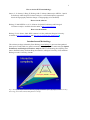
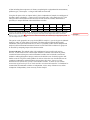
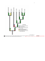
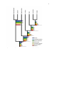
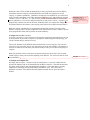
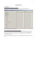
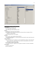
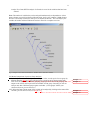
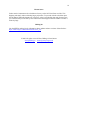
MANUAL
SEEVA Software
Spatial Evolutionary and Ecological Vicariance Analysis
Beta version: ver. 0.33
released Nov 1, 2008
By Einar Heiberg & Lena Struwe
websites: seeva.heiberg.se or www.rci.rutgers.edu/~struwe/seeva
Important note: This software is a work in progress and the full version not yet released. We
appreciate any feedback and suggestions for improvement.
SEEVA is a free software product to all non-commercial and academic users. If you are a
commercial user (private company or similar), please contact us for licensing fees.
© 2008 Einar Heiberg & Lena Struwe. All rights reserved.
[email protected]
[email protected]
2
How to cite the SEEVA methodology:
Struwe, L., P. Smouse, S. Haag, E. Heiberg, & R. G. Lathrop. (Manuscript). SEEVA – Spatial
Evolutionary and Ecological Vicariance Analysis: a new interdisciplinary approach to
historical biogeography and niche changes. J. Biogeography (to be submitted).
How to cite the software:
Heiberg, E. 2008. SEEVA ver. 0.33. Software for Spatial Evolutionary and Ecological
Vicariance Analysis. Available from the author at http://seeva.heiberg.se.
How to cite the manual:
Heiberg, E. & L. Struwe. 2008. SEEVA manual. On-line publication, Rutgers University.
Available at http://seeva.heiberg.se and http://www.rci.rutgers.edu/~struwe/seeva.
Introduction and Methodology
This software package, authored by Einar Heiberg (www.heiberg.se), processes data gathered
from species or individuals in a spatial, taxonomic, and/or phylogenetic context using the Spatial
Evolutionary and Ecological Vicariance Analysis (SEEVA) methodology developed by Lena
Struwe, Richard Lathrop, and Scott Haag Peter Smouse, at Rutgers University, USA, and Einar
Heiberg at Lund’s University, Sweden.
Fig. 1. Showing the complex interaction between geography (distribution. space), phylogeny (evolution, ancestry),
and ecology (environment, climate) through time for a lineage.
3
In contrast to traditional vicariance biogeography, which assumes geographic separation of
populations, the Spatial Evolutionary and Ecological Vicariance Analysis approach allows
researchers to look at ecological vicariance (differences) of sympatric and allopatric species and
clades. This method can utilize GIS-derived dataset of collection-associated ecological and
environmental data in combination with phylogenetic data to investigate trends in speciation
using statistical methods with spatial interpretations. The method can also be used for many
other kinds of comparisons between groups and clades, in areas such as co-evolution, diseases,
morphological evolution, and niche comparisons.
Generally, SEEVA works by using measurements gathered from individuals of species or
populations, and these measurements are then analyzed statistically for differences between
groups (species) and/or clades. Two statistical test have been employed, the chi-square test and
Fisher’s Exact test (the latter to provide a better p-value for tests with small sample sizes).
Environmental variables are divided into categories either as non-ordered, qualitative sections
(e.g., soil types) or ordered, quantitative sections representing quartiles of the total amount of
data (e.g., precipitation categories). A statistical test is performed to investigate if the distribution
of species or monophyletic clades in different categories of environmental variables shows a
random or non-random pattern, with taxonomic group vs. counts for collections for the
categories for one variable in an X x Y multi-way table.
variable
category 2 category 3
category 4
number of
observations
category 1
species/clade A
0
10
16
21
species/ clade B
10
15
9
0
Table. 1. Example of X x Y multi-way table showing skewed character state distributions for two different groups
using 4 states for one particular variable. The numbers are number of observations. i.e., collections.
A non-random (skewed) pattern a stronger association for an environmental character state(s)
with a specific group/clade, both historically (evolutionary) and presently. The classification of
the environmental variables is rather coarse, but these tests provide a way of looking for broad
patterns.
Examples of questions that can be analyzed with the SEEVA method include:
• Which environmental variable show the biggest difference between two sister groups, or two
sympatric species?
• What patterns in soil types do you see as you move up in the phylogeny of a group?
• Are species in dry-season areas derived from wet-season areas?
• Is long-distance dispersal associated with changes in ecological traits?
• What came first, higher rainfall or higher elevation, in a particular clade?
• Do allopatric sister species show larger ecological divergence than sympatric sister species?
The SEEVA method can be enhanced when combined with dispersal-vicariance analysis
(DIVA), ancestral area analysis, dating methods, geographic mapping of populations,
endangered species analysis, and ecological niche analysis. The method will work on any kind
4
of data including absence/presence of diseases, morphological or phytochemical measurements,
pollinator type, color morphs – as long as individuals are measured.
Using the chi-square value, an impact index (i) that is independent of sample size and degrees of
freedom is being calculated (i = square root of [(chi-square value / (df x sample size N)]). This
index provides a measurement for the skewness for each node and variable, and therefore a
possibility to compare different nodes and different variables.
species/clade
category category category category p chi2
df
impact
1
2
3
4
index
viridiflora
0
0
2
0
0.093473
3
0.430331
alata;hookeriana;connata
1
2
1
2
Table 2. Example of results table for one node (with one species vs. 3 species in the sister clades) and one variable,
showing to the right the character state distributions for two clades and their observed data (colletions). then to the
left the P-value from the chi-square analysis, the degrees of freedom, and the impact index number; all from the
SEEVA analysis. Note that in this particular case a Fisher’s Exact analysis is needed to get an appropriate p-value
since the sample sizes are so small.
The species can be grouped in two ways for the SEEVA analysis: 1) species-by-species (Manual
Analysis); and 2) by sister clades (Tree-based). The latter approach includes phylogenetic
information, since species data from two (or more, if a polytomy) clades will be compared and
analyzed, and environmental trends and reactions over the time of the evolution of a group can
be assessed by comparing impact values between nodes.
Caveats and notes: The method works with a minimum of one record for each species,
however, results based on such a small sample should be evaluated with caution. In general,
correlations between divergence and environmental variables can be inferred as trends and
tendencies within phylogenetic lineages, and not as the definite cause for the divergence until
further research. The generic null hypothesis for all tests is that the cross-classified factors are
completely independent, and the hypothesis driving the work is that: “Species or clade
distributions are influenced by specific environmental variables, as shown by non-random
associations of particular species or clades and their environmental situations”. It should not be
assumed that environmental variables are independent, in fact, many of them are not, and an
assumption of independency is not necessary for this analysis.
Borttaget: w
5
Fig. 2. Differences in distribution of 4 soil categories (one variable) throughout a phylogenetic tree. The numbers are
impact indices for each node, the bars indicate percentage of categories present in each sister group. The figure was
made in Powerpoint with customized graphs imported from Excel.
Borttaget: r
6
Fig. 3. Differences in impact indices for 7 environmental variables throughout a phylogenetic tree.
7
Download and Installation
(download website: http://seeva.heiberg.se)
The SEEVA program is written in Matlab. For you who do not have Matlab we have compiled
the application to a stand-alone application, so it can be run on any Windows computer. If you
want to run the software on other platforms such as Mac or Linux, please contact the Einar
Heiberg and you will then be provided with the source code so the software can be run from
Matlab on that particular platform.
The precompiled version runs on PC under Windows XP, Vista, NT, ME (but this program does
not work on Windows 98). You will need 500 MB free harddrive space and 256 MB RAM
memory.
1) Install Matlab Component Runtime
First a program called Matlab Component Runtime is required. This is essentially a small Matlab
installation, but can only be used to run precompiled applications. If Matlab Component Runtime
is already installed you can omit this step, but double check your version. This is found in
Windows control panel, under Add/Remove programs. Look for MATLAB Component Runtime
7.8 on the list (size 466 MB). If your Matlab Component Runtime version is less than 7.6, then
you need to uninstall the old first and then install the new program, see under 1.2 below).
Uninstalling the old one is done by clicking on its name in the list and select "Remove". You
need to be logged in as an administrator to do this.
1.1) Log in as administrator on your computer.
1.2) Download the file MCRInstaller_R2008a.exe (large file!!! 200+MB) from
http://seeva.heiberg.se.
1.3) Install Matlab Component Runtime (MCRInstaller_R2008a.exe) by double-clicking on its
icon. If the program asks you to install VCRedist_x86 as part of this installation – this is OK.
2) Download SEEVA
2.1) Download the file seeva.exe from http://seeva.heiberg.se.
2.2) Create a new folder (we suggest the name SEEVA) on your computer and place the file
seeva.exe in that folder.
Preparing the data files
3) Prepare Excel file with variables
Prepare an Excel file that has one column named SPECIES which will contain the taxon name
for each collection. For each collection, add environmental data either as quantitative
measurements (elevation, etc.) or qualitative (vegetation type). We used geolocated specimens
and ArcGIS to pull out environmental data from many base layers of data from sources such as
USGS, WORLDCLIM, etc. The species column has to be to the left of the columns with
variables you want to analyze. You can have additional columns with other data such as
collection ID, geolocation, etc. and this will not affect the analysis. The top row is the name of
each column. Do not have empty rows or columns inside you spreadsheet, but you can have
empty cells for missing data. .
Borttaget: Mb
8
Quantitative data will be divided up automatically in four groups from min to max in SEEVA,
with borders between categories currently defined so one fourth of all samples are in each
category, to optimize repeatability. Qualitative variables has to be modified by you in the Excel
sheet to include a minimum of two and a maximum of four states each, with each state not being
a number (A, B, C is OK, but 1, 2, 3 will not work, because if numerical SEEVA will treat the
data as quantitative). You can have longer descriptions as well (such as ‘forest’, ‘savanna’). The
program only reads the first sheet in the Excel workbook. Please see example files. Empty cells
are permitted and will be treated as a non existing value and will be excluded from the analysis.
Kommentar [A1]: Have you
tried with more? I have no
recollection of minimizing to 4?
Borttaget:
Note: For numeric variables they are automatically divided into quartiles. The ranges of the
quartiles are printed above all node comparisons in the output file (see below). In future versions
of the program these limits will be possible to encode manually.
4) Prepare the tree file (if needed)
A tree file is necessary if you want to base your analysis on topologies and comparisons of nodeby-node patterns. If you want to compare 2-5 groups/taxa without any particular topology, you
can do a manual analysis without a tree file.
The tree file should be in the NEXUS format and end with .nex (text-only file). You can have
several trees in your treefile, but you can only analyze one at the time in SEEVA. Polytomies in
the trees are allowed, but will affect your statistical analysis since you will have more groups to
compare.
Note: Taxon names in the tree file must correspond exactly to the Excel sheet’s species name
column. Root or orient your tree before importing it into SEEVA. You will not be able to reroot
it inside SEEVA.
5) Example and template files
One large (Macrocarpaea, +50 species) and one small (Tachia, 13 species) example files are
provided as templates and can be downloaded on the SEEVA websites. Note that this data does
not reflect actual scientific data and phylogenetic hypotheses. These data matrices are only
templates for formatting, training, and testing by the SEEVA users. None of the data is
published or accurate. More details about the template/example files are given later in this
manual.
Borttaget: Also, sometimes
9
Running SEEVA
6) Run SEEVA
6.1) Double click on seeva.exe to start SEEVA.
If you get a warning about the publisher being unknown, ignore this and click OK.
Fig, 4. The user interface when you open SEEVA:
6.2) Load Data File and Tree File (the latter is optional):
Click on Open Data file pushbutton to select a data file to load. To load a tree, select Load Tree
in the Tree Analysis panel. This step is only required if you intend to run a tree (phylogenybased) analysis. If the tree file contains more than one tree then you will be prompted and can
select which tree to import.
Species and variables can be selected by clicking the mouse and holding down the Shift or Ctrl
keys.
10
Fig, 5. The user interface when you have opened a data file:
6.3) Overview of windows interface and options:
Menu options:
File: open and clear data file, quit
Tree: open, analyze, and plot tree
Help: Home page, About, Submit bug report
Buttons:
Open Data File: Opens Excel sheet with data.
Store Messages to File: Opens a log file for error messages and run commands. (This is
helpful for troubleshooting.)
Finish Writing Messages: Closes log file
Windows:
Species: Species names pulled from Excel data file
Data columns: Lists columns of variables pulled from the data file, listed in order from left to
right in the data file.
Manual Analysis:
Group 1-5: Add species to each group as you want; hold shift or Ctrl key to select more than
one species at a time. Select all species you want first, then add them, or the selection
will overwrite the previous selection.
Select variables to analyze in right window.
Click Manual analysis to compare (at least 2 groups are needed, one variable is minimum).
Tree Analysis:
Load Tree: Loads tree file
Plot Tree: Shows tree
11
Analyze Tree: Runs SEEVA analysis of all nodes in a tree for the variables that have been
selected
Note: The number of variables that can be analyzed simultaneously are dependent on 1) how
many columns you can fit into the Excel Results sheet, and 2) your computer’s RAM memory.
We have successfully run analyses with up to 10 variables at the time. You can analyze your
variables in batches and then combine the results in Excel for a complete overview.
Fig. 6. Example of Tree shown inside SEEVA. Numbers refer to each node’s number.
6.4) Manual comparison of species (Group Analysis)
6.4.1) In the Species window select species to compare. Select several species for one group by
holding down the Shift or Ctrl key. All species for a group has to be selected at the same
time. Click on Group 1 to set the first grouping, on group 2 to set the second grouping. The
output result will list which species that are member of what group. Currently you can not
analyze more than 5 different groups against each other. (“Clear groups” deletes your
selection of taxa so you can start over.)
6.4.2) Select the Data Column name of the variable to be analyzed by clicking on the name of the
variable (you can select several, use Shift or Ctrl).
Borttaget: SHIFT
Borttaget: TRL
Borttaget: HIFT
Borttaget: TRL
12
6.4.3) Click on Group Analysis. The analysis will be run and the results will be copied to the
Clipboard. Open an empty Excel sheet, and select Edit - Paste or Ctrl+V to paste the
Clipboard data into Excel. Save the Excel file.
Fig, 7. The user interface when you have loaded a Data file, a Tree File, and selected species for your Manual
Analysis and selected 4 variables for analysis.
6.5) Comparison of species based on a phylogenetic tree
6.5.1) Select Load tree in the Tree menu.
6.5.2) To see the tree, use Plot Tree in the Tree menu. This tree can be printed to a printer or a
pdf file (if you have Adobe Acrobat or Distiller), and you can also zoom the tree under Print
Preview. Nodes are indicated with numbers.
6.5.3) Select one to several data columns for the variables you want to analyze.
6.5.4) Under Tree menu, select Analyze tree. You will be prompted to save the results in a new
Excel file. You cannot add data to an existing Excel file, so give each results file a new
name.
6.6) Understanding the data output
Open Excel and the results file. The setup of the results file is the same for Manual Analysis as
for Tree Analysis.
13
Fig. 8. Results output with explanations in red. See Tachia example files for further explanation.
The data can now be graphed and arranged in various tables in Excel for easy comparison. It can
be overlaid on a map, or used for plotting or shown as trend lines throughout a phylogeny; the
possibilities are endless.
Example files:
Tachia (13 species)
TachiaRAWDATA.xls (Data File: environmental data for 150 collections and 4 variables (2
quantitative, 2 qualitative), as well as collection ID numbers and geolocation data.)
TachiaTREE.nex (Tree File: in NEXUS format)
TachiaMATRIXTREE.nex (Tree File: datamatrix and tree file in Nexus format)
TachiaRESULTSManualAnalysis.xls (Results File: comments added)
TachiaRESULTSTreeAnalysis.xls (Results File: comments added)
Macrocarpaea (62 species, including outgroups)
MacrocarpaeaRAWDATA.xls (Data File: environmental data for 800 collections and 5 variables
(1 quantitative, 4 qualitative), as well as collection ID numbers and geolocation data.)
MacrocarpaeaMATRIXTREE.nex (Tree File: datamatrix and tree file in Nexus format)
MacrocarpaeaRESULTSManualAnalysis.xls (Results File)
MacrocarpaeaRESULTSTreeAnalysis.xls (Results File)
14
Known issues
Under certain circumstances the calculation of exact p-value for Fisher Exact test fails. This
happens particularly when calculating larger polytomies. To proceed with the calculation press
the OK button. When this happens no value for p-value is provided for that node. In most cases
you can then safely use the chi2 p-value instead since this happens when the number of items is
relatively large.
Mailing list
Join the SEEVA mailing list for information about updates and new versions. Subscribe here:
https://email.rutgers.edu/mailman/listinfo/seeva_list
© 2008. All rights reserved. Einar Heiberg & Lena Struwe
[email protected] [email protected]