Download Ronquist 1996_DIVA user manual

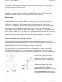
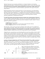
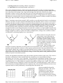
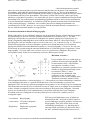
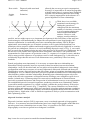
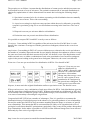
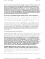
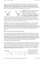
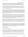
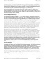
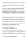
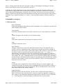
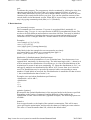
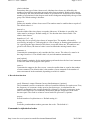
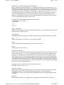
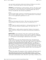
DIVA 1.1 User’s Manual
Page 1 of 21
Swedish | English | Uppsala University | Home | Research | Information | Staff
DIVA 1.1 User’s Manual
5 November, 1996
© Fredrik Ronquist, Dep. Systematic Zoology, Evolutionary Biology Centre, Uppsala University,
Norbyvägen 18 D, SE-752 36 Uppsala, Sweden, email: [email protected].
Introduction
DIVA is a simple program for reconstructing ancestral distributions in a phylogeny using dispersalvicariance analysis (DIVA), a method in which ancestral distributions are inferred based on a threedimensional cost matrix derived from a simple biogeographic model . Unlike other methods in
historical biogeography, DIVA does not assume anything about the shape or existence of general
biogeographic patterns. Therefore, DIVA is particularly useful in reconstructing the distribution
history of a group of organisms in the absence of a general hypothesis of area relationships ("taxon
biogeography"). The method remains applicable even when area relationships are expected to be
reticulate rather than hierarchic. Dispersal-vicariance reconstructions obtained for different groups of
organisms inhabiting the same areas may be collated and used to infer general biogeographic
patterns ("area biogeography"). For this purpose, the DIVA program provides several ways of
summarising information in sets of taxon-based reconstructions.
Citation, availability, and disclaimer
Cite this manual and the DIVA program as "Ronquist, F. 1996. DIVA version 1.1. Computer
program and manual available by anonymous FTP from Uppsala University (ftp.uu.se or
ftp.systbot.uu.se)". The program and manual may be copied and distributed freely provided that the
source of results or ideas is cited. The source code is available from the same FTP sites and may be
copied, modified and recompiled as desired. There are no warranties, neither express nor implied.
The program may contain bugs that will crash your system or overwrite sectors of your hard disk. Be
sure to keep backups of all important documents and software, and save all your work before
launching DIVA.
Installation
There are three versions of the program: (1) DIVAppc runs natively on Power Macs; (2) DIVA68K
runs on the old Macintoshes (system 7.0 and later) and in emulated (slower) mode on Power Macs;
(3) DIVA.exe is for 32-bit Windows systems, including Windows 3.x with Win32S installed,
Windows95, and Windows NT. The different versions of DIVA behave almost identically and will
only be distinguished herein when necessary.
DIVA requests 1 MB of memory but it will run successfully with much less. However, the amount
of available memory may limit the possibilities of obtaining exact solutions for complicated
problems. To install the program, simply copy it to the desired folder (directory). For simplicity, I
http://www.ebc.uu.se/systzoo/research/diva/manual/dmanual.html
30/03/2009
DIVA 1.1 User’s Manual
Page 2 of 21
will assume in this manual that all batch files and NEXUS files that DIVA works with are in the
same folder (directory) as the program.
Bugs in pre-release versions
Pre-release versions of DIVA (versions 0.9, 1.0, 1.0a, and 1.0b) contain a bug that, with a low
probability, causes the program to include spurious distributions in the optimal reconstructions.
Results based on these versions of DIVA should therefore not be published.
Background
Analytical protocols in historical biogeography and coevolution may be divided into event-based
methods and pattern-based methods. Brooks parsimony analysis , ancestral area analysis and
component analysis are examples of pattern-based methods. These methods measure the fit of data to
a particular coevolutionary or biogeographic scenario in abstract units like "items of error",
"reversals" or "homoplasy". Therefore, pattern-based methods are prone to give results that imply
contradictory or highly improbable underlying mechanisms, such as derived species evolving into
their ancestors or irreversible dispersal away from an ancestral area . By explicitly basing
biogeographic and coevolutionary inference on models of the events involved, such contradictions
can be avoided. Event-based methods have been criticised because the accuracy of the result depends
on the validity of the model . However, there is no fundamental difference between the approaches in
this respect, since the success of pattern-based methods, like that of event-based methods, is
ultimately determined by the relation between the details of the method and the nature of the
processes being inferred.
Event-based methods in coevolutionary inference
Historical biogeography shares many fundamental concepts and ideas with macroevolutionary
comparisons of host and parasite phylogenies. Because event-based methods were first developed for
coevolutionary problems, a digression on coevolution may serve as a good introduction to the
fundamental issues involved in event-based biogeographic reconstruction.
A common problem in coevolutionary inference may be formulated as follows: Given a host
phylogeny, a parasite phylogeny, and an association matrix defining the species or terminal taxa that
are currently associated (Fig. 1), the task is to reconstruct the history of the association or, more
specifically, which ancestral parasites were associated with which hosts. To be able to distinguish all
branches in the host and parasite trees, we will assume that each branch represents a separate species.
Ronquist and Nylin were the first to
propose an event-based coevolutionary
method to accomplish this task. They
recognised four types of events in their
model:
z
z
z
z
fewer members)
Duplication (called broadening of the
association by Ronquist and Nylin)
Exclusion (parasites being excluded from
or actively avoiding certain hosts)
Colonisation (parasites adding a new host
species to the range of hosts attacked)
Successive specialisation (narrowing of
the association after speciation to include
http://www.ebc.uu.se/systzoo/research/diva/manual/dmanual.html
30/03/2009
DIVA 1.1 User’s Manual
Page 3 of 21
The basic idea was to use cost matrix optimisation to reconstruct the history of associations
(Ronquist and Nylin 1990). To do that it is necessary to specify a relative cost for each of the events
in the model, the cost being inversely related to the likelihood of the event occurring. Once the costs
have been determined, it is possible to find the minimum-cost reconstruction, which would be the
most likely (most parsimonious or maximum likelihood) explanation for the origin of the pattern
being analysed.
Ronquist and Nylin focused on systems where the sets of associated species were determined by
parasite and host traits ("active associations"). If these traits remained unchanged, host or parasite
speciation would result in duplication, i.e., broadening of the association to include more members .
Thus, duplications may be considered the null model in coevolutionary inference and associated with
a cost of zero, just like maintenance of a trait (no change) is the null expectation in ordinary
parsimony optimisation of morphological characters.
To simplify the problem further, Ronquist and Nylin introduced the assumption that each parasite
occupies a single host at any single point in time (the one-host-per-parasite assumption). This would
seem a reasonable assumption for intimate associations, the systems that would be most likely to be
historically constrained . Under the one-host-per-parasite assumption, only three kinds of events are
possible in optimal reconstructions :
z
z
z
Duplication (null expectation)
Host switching (colonisation of a new host and exclusion from the old host)
Host tracking (equivalent to successive specialisation)
The importance of the one-host-per-parasite assumption is that it allows one to use standard cost
matrix optimisation methods, which assume that ancestors are monomorphic, to map hosts onto the
parasite phylogeny. Note that it would not be possible to do it the other way round. Even under the
one-host-per-parasite assumption, it is permissible for several parasites to attack the same host, and
standard techniques could therefore not be used to map parasites onto the host phylogeny.
If duplications are expected, then we need only determine the cost of host switches relative to that of
tracking events. Assume that this value is given. Then a step matrix specifying the cost of moving
between different ancestral and/or extant hosts can be constructed , and standard optimisation of this
complex host matrix character onto the parasite phylogeny gives the minimum-cost reconstruction of
the history of the association. By using a suitable fit function, it is possible to compare the mapping
results obtained with different relative switch costs and find the optimal switching/tracking cost ratio
for a particular association .
A simple example may illustrate the construction of a host step matrix (Fig. 2). There are only two
host species, A and B, and their ancestor, C. To move from A or B to C is impossible (associated
with infinite cost), because C is the ancestor of A and B and ceased to exist when A and B were
formed. To move from A to B or vice versa costs one host switching event (cost s). To move from C
to B or from C to A implies one host tracking event (cost t). Finally, remaining on the same host
after speciation represents duplication and costs nothing (the diagonal row of zeros).
Page recently proposed a different event-based
method to reconstruct the history of host-parasite
associations under the one-host-per-parasite
assumption. He recognised four different types of
events in his model:
z
z
Duplication
Host switching (colonisation and exclusion
combined)
http://www.ebc.uu.se/systzoo/research/diva/manual/dmanual.html
30/03/2009
DIVA 1.1 User’s Manual
z
z
Page 4 of 21
Sorting events (host tracking without cospeciation)
Cospeciation (host tracking through cospeciation)
The events considered in Page’s model correspond closely to those in the cost matrix approach
developed by Ronquist and Nylin; the only important difference is that Page separates host tracking
into cospeciation and sorting events. Page acknowledged the difficulties involved in trying to
determine a relative cost for each of the four types of events and suggested, as a first simple
approach, to choose reconstructions that maximise the number of cospeciations. He also presented
algorithms for optimising this criterion, implemented in the program TreeMap (available from Rod’s
home page: http://taxonomy.zoology.gla.ac.uk/rod/rod.html).
Page’s "maximum cospeciation method" (MC) provides a powerful analytical tool in coevolutionary
inference, but there are some important limitations that one should be aware of. First, it is necessary
to assume that host switches are always associated with speciation (these speciation events cannot
then be cospeciations) and that only one of the two resulting daughter species shifts to a new host. If
these constraints were not imposed, it would be possible to assign cospeciation events to all of the
ancestral parasite nodes regardless of the host associations of the terminals by simply allowing
enough host shifts on the terminal branches. Second, MC is similar to a clique method in that it only
considers one type of events. Thus, the maximum cospeciation reconstruction will be preferred even
though it might be possible to reduce the number of duplications, sorting events, and host switches
considerably by assuming slightly fewer cospeciations .
Third, one has to accept the focus on
cospeciation events rather than on
tracking events in general. In activeassociation systems, changes in the
association matrix would necessarily
be tied to changes in parasite and host
traits, regardless of whether or not the
cause of these changes were
cospeciation . Thus, tracking events
would be of primary importance in such systems, not cospeciation events. With this perspective,
spatially separated parasites and hosts really represent question marks in the association matrix - we
do not know whether they would be associated had they been in contact . In MC analyses, on the
other hand, it must be acknowledged that the cause of cospeciation may be biogeographic (common
dispersal barriers) rather than coevolutionary (changes in host and parasite traits), particularly in the
analysis of passive-association systems.
Finally, the algorithms presented by Page may produce spurious results in some cases. The reason is
that some combinations of host switches that are contradictory are not prohibited in Page’s
algorithms, not even in the "exact" algorithm . The problematic combinations include switches from
an original host via an intermediate host to hosts that had gone extinct before the appearance of the
original host (Fig. 3a). This problem is currently being addressed (Page, pers. comm.). The same
type of problem occurs in mapping of a host step matrix onto a parasite phylogeny. In this context it
can be solved by dividing branches into time segments (Fig. 3b). Switches backwards in time across
segment borders are then prohibited by associating them with infinite cost .
Like the method developed by
Ronquist and Nylin , MC can be
formulated as a cost matrix
optimisation method. Because
there is a distinction between
cospeciations and simple tracking
events in MC, it is necessary to use
http://www.ebc.uu.se/systzoo/research/diva/manual/dmanual.html
30/03/2009
DIVA 1.1 User’s Manual
Page 5 of 21
a three-dimensional step matrix,
where one axis represents the host of the ancestor and the other two the hosts of the immediate
descendants, rather than the standard two-dimensional matrix (Fig. 4). The two descendants are
equivalent making half the matrix redundant, but the matrix is asymmetric in that the ancestor cannot
be substituted with any of the descendants. This matrix is filled with "benefit" values specifying
whether a cospeciation is possible (1) or impossible (0) given a certain combination of ancestral and
descendant hosts. By using dynamic-programming algorithms similar to those used in optimisation
of a two-dimensional step matrix, it is possible to find the optimal reconstruction of ancestral hosts
in the parasite phylogeny . Ordinarily, one would be interested in finding the minimum-cost
reconstruction(s). In MC, however, we are trying to find the maximum-benefit reconstruction, i.e.,
the one with the maximum number of cospeciations.
Event-based methods in historical biogeography
Much of the theory of coevolutionary inference can be translated directly to historical biogeography
by substituting area for host. Take the problem formulation in coevolution (Fig. 1). The host
phylogeny corresponds to a general area cladogram, the parasite phylogeny to a phylogeny of a
group of organisms inhabiting those areas, and the association matrix to a distribution matrix
specifying for each area whether a species occurs in the area (1) or is absent (0) (Fig. 5). The task in
historical biogeography is often to formulate a general area cladogram from a set of organism
phylogenies and the associated distribution matrices ("area biogeography"). However, we may also
be interested in reconstructing the ancestral distributions of a particular group of organisms ("taxon
biogeography"). If, in the latter case, we have access to a general area cladogram, the problem
corresponds exactly to that in coevolutionary inference discussed previously.
Maximum vicariance
Let us examine MC as it would apply to
problems in historical biogeography. The
events translate easily: cospeciations
correspond to vicariance events,
duplications to sympatric speciation, host
switches to dispersal and sorting events
to extinction (Table 1). Since
cospeciations are substituted with
vicariance events, it would seem
appropriate to refer to the method as the
"maximum vicariance method" (MV).
The assumption that there is a host phylogeny, i.e., a hierarchical set of host relationships, translates
to an assumption that there is a general, hierarchical set of area relationships (a general area
cladogram). The one-host-per-parasite assumption corresponds to a one-area-per-species assumption.
This means that ancestral species are allowed to occur in single areas or in multiple areas postulated
to have formed a contiguous region in the past according to the general area cladogram. Ancestral
species are not allowed to occur simultaneously in areas that could not have been contiguous
according to the area cladogram, nor are they allowed to be restricted to a smaller part of a
contiguous region.
Coevolution
Biogeography
Cospeciation Vicariance (allopatric
speciation)
Duplication
Duplication (sympatric
speciation)
MV has several limitations, some of which are
inherited from MC, and some of which relate to
special challenges posed by problems in historical
biogeography. First, MV suffers from several
constraining assumptions, e.g., that dispersal is
associated with speciation (see discussion above
for MC), and that widespread ancestors are not
http://www.ebc.uu.se/systzoo/research/diva/manual/dmanual.html
30/03/2009
DIVA 1.1 User’s Manual
Host switch
Dispersal (with associated
extinction)
Sorting
event
Extinction
Page 6 of 21
allowed (the one-area-per-species assumption).
Second, it is impossible to do taxon biogeography
with MV unless there is a general area cladogram
available. Reconstructing ancestral areas using
MV is simply inappropriate in the absence of a
general hypothesis of area relationships.
Third, there is no available,
automated search strategy for
finding the general area
cladogram with the maximum
number of vicariance events from
a set of organism phylogenies
and associated distribution
matrices. However, such
analyses would certainly be
possible, and we might expect to see important developments in this field. Many of the usual tree
search strategies could undoubtedly be adapted for such problems in area biogeography. MV
character optimisation is considerably more time-consuming than ordinary Fitch or Wagner
optimisation, necessitating the use of heuristic searches even for quite limited problems, but
techniques such as stepwise addition and branch swapping would be directly applicable to searches
for general area cladograms. However, to avoid conflicting dispersal events (cf. Fig. 3), one would
have to search for an optimal solution not only in the universe of all possible area cladograms, but in
the universe of all possible time-segmented area cladograms. Since there is one possible time
segmentation for each sequence of speciation events (i.e., sequence of vicariance events), and there
may be many possible sequences of speciation events for each cladogram (Fig. 6), this universe is
considerably larger than the universe of all dichotomous trees, particularly if there are many
terminals.
Fourth, and perhaps most importantly, it is necessary to assume that area relationships are
hierarchical. Being organisms, hosts are expected to show hierarchical ancestor-descendant
relationships. Areas, on the other hand, are not subject to hierarchical cladogenesis Areas change
configurations with time as terranes are created, fragmented, dislocated, distorted and destroyed.
Through these events, dispersal barriers that affect many groups of organisms simultaneously appear
and disappear. Yet, we cannot expect these processes to produce hierarchical area relationships more
often than they produce reticulate relationships. Branching area relationships appear only as the
result of the successive appearance of dispersal barriers dividing a once contiguous region in ever
smaller, isolated areas. Common geological events such as establishment of contact between
previously separated land masses and retrogression of midcontinental seaways create opportunities
for nonrandom dispersal of terrestrial organisms, producing reticulate area relationships. Similar
events affect marine organisms. For a simple example, consider the geologic history of the major
Holarctic regions in the Cenozoic (Fig. 7; simplified). The current continents were formed from
separate western and eastern areas, which were previously joined into palaeocontinents combining
the areas differently . The distribution history of Holarctic organisms should reflect the reticulate
geologic history. Application of MV to Holarctic organisms is likely to yield reconstructions with
little explanatory power.
Dispersal-vicariance analysis
Dispersal-vicariance analysis (DIVA) represents a new event-based approach to biogeographic
inference . It reconstructs ancestral distributions based on a simple biogeographic model that does
not take general area relationships into account. Thus, it is possible to use DIVA in taxon
biogeography even when no general area cladogram is available.
http://www.ebc.uu.se/systzoo/research/diva/manual/dmanual.html
30/03/2009
DIVA 1.1 User’s Manual
Page 7 of 21
The premises are as follows: Assume that the distributions of extant species and their ancestors can
be described in terms of a set of unit areas. The optimal reconstruction of ancestral distributions is
obtained by optimisation of a three-dimensional cost matrix derived using the following simple
rules:
1. Speciation is assumed to be by vicariance separating a wide distribution into two mutually
exclusive sets of areas. This event costs nothing.
2. A species occurring in a single area may speciate within the area by allopatric (or possibly
sympatric) speciation giving rise to two descendants occurring in the same area. The cost is
zero.
3. Dispersal costs one per unit area added to a distribution.
4. Extinction costs one per unit area deleted from a distribution.
It is possible to compare DIVA and MV event by event as follows:
Vicariance. Costs nothing in DIVA regardless of the unit areas involved. In MV there is a unit
benefit if the vicariance event agrees with the general area cladogram, otherwise the event is not
allowed.
Duplication. Costs nothing in DIVA if it occurs within one area, otherwise the cost is equivalent to
the number of secondary dispersals needed for two initially allopatric descendants to come to occupy
the same set of unit areas that their ancestor did. In MV, the benefit is zero if the duplication occurs
within one unit area, or within a combination of unit areas postulated to have formed a contiguous
region in the past according to the general area cladogram. Otherwise, the event is not allowed.
Extinction. Costs one per area deleted in a distribution in DIVA. Zero benefit in MV.
Dispersal. Costs one per area
added to a distribution in
DIVA. In MV, dispersal is only
allowed if it is associated with
speciation. A descendant
lineage may then occupy a new
area or a new region of areas
postulated to be contiguous in
the general area cladogram. The
sister species is not allowed to
disperse; it must retain the original distribution until next speciation event. The benefit is zero.
Widespread ancestors. Any combination of unit areas allowed in DIVA. Only distributions agreeing
with the general area cladogram allowed in MV. Widespread terminals are problematic in MV; they
can be treated either as composite groups with separate lineages, each restricted to a single unit area,
or as cases of uncertainty concerning the original area.
Compared with MV, DIVA has a number of advantages. First, it is possible to reconstruct the
distribution history of individual groups in the absence of a general hypothesis of area relationships.
Second, the model used in DIVA does not assume anything about the shape or existence of general
area relationships. This means that DIVA reconstructions are likely to fit a hypothesised series of
geological events better than MV optimisations, particularly if the events do not produce hierarchical
area relationships. It also makes it possible to use DIVA when different lineages have been affected
differently by some series of geological events.
http://www.ebc.uu.se/systzoo/research/diva/manual/dmanual.html
30/03/2009
DIVA 1.1 User’s Manual
Page 8 of 21
Dispersal-vicariance reconstructions for different groups of organisms inhabiting the same set of unit
areas may be assembled and compared to allow testing of hypotheses about general biogeographic
events , regardless of whether these events produced hierarchically nested area relationships.
However, it is important to consider exactly under what circumstances we might be able to retrieve
reticulate area relationships. Assume that we have two sister species which occur in area A and B,
and that we infer correctly that their ancestor occurred in A+B (Fig. 8). According to the reticulate
biogeographic scenario (to the left in Fig. 8), we would expect this ancestor to stem either from A or
B before the union of the areas. The only chance to determine this centre of origin correctly would
be if some related species stemming from the same centre of origin remained unaffected by the union
of A with B. Thus, reticulate area relationships can only be detected if some species fail to expand
their distributions despite the disappearance of dispersal barriers.
DIVA attempts to find such archaic remnants and, if they are found, utilises the information in
retrieving reticulate area relationships. MV, on the other hand, assumes that narrowly distributed, old
lineages are the result of extinction of more widely distributed ancestors. A possible disadvantage
with the DIVA approach is that extinction is not modelled realistically. Actually, extinction events
will never appear in dispersal-vicariance optimisations unless geographic constraints are used to
modify the original cost assignment rules. MV, on the other hand, may make too frequent use of
extinction events in explaining away misfits to a hierarchic general area cladogram.
Think of three-dimensional cost matrices as the generic approach in historical biogeographic and
coevolutionary inference. DIVA and MV represent simple methods falling within this framework,
just like Fitch and Wagner parsimony represent special cases of character reconstruction based on
cost matrices . In the future, we will undoubtedly see more sophisticated uses of three- and twodimensional step matrices in coevolution and historical biogeography. An important challenge in
historical biogeography will be to incorporate geological constraints into the model, such that
reticulate and hierarchic biogeographic scenarios can be tested directly against each other on
equivalent terms.
Some pitfalls in dispersal-vicariance optimisation
Ancestral areas. When using DIVA to reconstruct the ancestral area or centre of origin of a group of
organisms (Bremer 1992), it is important to remember that optimisations become less reliable as you
approach the root node. This is because the tree that you work with represents a small part of the tree
of life, and the globally optimal states of the basal nodes in your subtree are particularly heavily
influenced by the rest of the tree of life. The root node state, i.e., the ancestral distribution, is the
least reliable in your entire tree. In DIVA, this uncertainty will be manifested as a tendency for the
root node distribution to be large and include most or all of the areas occupied by the terminals. If
you are interested in more reliable estimates of the distribution of the root node, you should include
additional outgroups in the analysis such that the node is no longer the root node. Alternatively, it
might be useful to examine the effects of imposing constraints on the maximum number of unit areas
allowed in ancestral distributions (using the maxareas option of the optimize command in DIVA).
Using this approach, we are asking the question: "If this group had a restricted distribution in the
past (maximally n unit areas), what is the most likely ancestral distribution of the group?".
Terminals are higher taxa. If the terminals in an analysis are higher taxa, such as genera or
families, it is important to recognise that one cannot simply add the distributions of the species
belonging to the higher taxon. A higher taxon should be coded for the likely ancestral distribution,
not as being distributed in all areas where descendants occur. The problem is exactly the same as that
which appears with polymorphic higher taxa in the optimisation of morphological characters. If the
taxon is coded for all states occurring in the taxon, information important for the optimisation of
ancestral states will be lost.
There are three approaches one could use to deal with widespread higher taxa. First, one might try to
http://www.ebc.uu.se/systzoo/research/diva/manual/dmanual.html
30/03/2009
DIVA 1.1 User’s Manual
Page 9 of 21
resolve lower-level relationships within the taxon and use these to reconstruct the likely ancestral
distribution. Second, one might infer likely ancestral distributions using the common-equalsprimitive criterion. Some caution is needed here, but if common is interpreted as common in basal
lineages, the criterion is clearly applicable. Third, it is possible to code the higher taxon as being
distributed in all areas where descendants occur, and use the maxareas option in DIVA to restrict the
number of unit areas that may have been occupied by any ancestral species.
Ambiguous events. Frequently there are several
alternative distributions at an ancestral node.
However, even when there is a single,
unambiguous state for each node in the tree,
there may be several equally costly combinations
of events that can explain these distributions.
Consider a pattern for which the single optimal
reconstruction implies that the descendant distributions resulted from vicariance followed by
secondary dispersal across the primary dispersal barrier (Fig. 9). The vicariance might have involved
separation of AB from CDE, with secondary dispersal of the left descendant into C (Fig. 9a), or
separation of ABC from DE, with secondary dispersal of the right descendant into C (Fig. 9b). Both
alternatives include one vicariance event and one dispersal event.
Polytomies. The current version of DIVA can only handle fully bifurcate trees. To infer ancestral
areas in polytomous cladograms, under the assumption that the polytomies represent uncertainty
(soft polytomies), it is necessary to enter all possible, fully bifurcate trees separately, and then
summarise the results. If the polytomous tree is a consensus tree, it would be more appropriate to run
DIVA separately on each of the trees from which the consensus was calculated. In some cases it may
be possible to combine taxa in polytomies with the same distribution into a single taxon to reduce the
number of arbitrary resolutions. Future releases of DIVA may be able to handle soft and hard
polytomies.
Dispersal-vicariance analysis and area biogeography
DIVA provides several features for summarising information in sets of reconstructions. The most
basic functions simply summarise the frequency of events such as particular vicariance or dispersal
events. The more advanced functions sort the events into time classes based on estimated dates for
the ancestral nodes. If there is some source of branch length estimates, the node ages can be entered
manually (using the "nodeage" command). DIVA can also calculate rough node ages using a simple
"speciation level measure" , which is based on the maximum number of nodes separating a particular
node from any subtended terminal, including the node itself (Fig. 10). This corresponds to the
maximum number of speciations, as evidenced by the cladogram, separating the ancestor
corresponding to the node from any terminal.
Several additional features in DIVA facilitate compilation of information in sets of reconstructions.
If the ages of the ancestral nodes in two cladograms are not comparable, it is possible to provide the
age of the root node in each group (by default set to 1.0) to calibrate the ages of the ancestral nodes.
If one of the source cladograms has one or more polytomies, all possible resolutions may have to be
entered separately to allow incorporation of the data in summary statistics. To avoid weighting
polytomous groups more heavily than others, such arbitrary resolutions can be downweighted (the
weight of each reconstruction is set to 1.0 by default).
Ancestral nodes commonly
have several, equally optimal
ancestral distributions.
Summary statistics can be
calculated only for those nodes
http://www.ebc.uu.se/systzoo/research/diva/manual/dmanual.html
30/03/2009
DIVA 1.1 User’s Manual
Page 10 of 21
with single (unambiguous)
distributions, or for all nodes. In the latter case, the program goes through all possible, equally
optimal reconstructions. Each reconstruction is then weighted such that the sum of all
reconstructions is unity. Thus, an event occurring in all reconstructions will obtain a frequency of
1.0, whereas an event occurring in only one reconstruction of 20 will obtain a frequency of 0.05.
Even when the distribution assignments are unequivocal, there may be several, equally optimal
combinations of events producing these distributions as noted above (Fig. 9). For each of these cases,
the program goes through all possible combinations of events, and weights each combination of
events in proportion to the number of possibilities. Thus, if there are two possible events (Fig. 9),
each event is assigned the frequency 0.5.
The age of vicariance events and distributions correspond directly to the age of the ancestral node to
which they belong. Dispersal events, however, occur along internodes and may therefore be assigned
any date from the age of the ancestral node incident to the branch to the age of the descendant node
incident to the branch. DIVA arbitrarily uses the age of the ancestral node. DIVA only deals with
dispersals in which both the ancestral and the target areas can be identified unambiguously. Thus, the
dispersals considered in the summary statistics only include those where an ancestor occurring in a
single area colonises a second area.
When using DIVA in area biogeography, the possible existence of reticulate area relationships must
be acknowledged. Thus, it is inappropriate to use the term ‘general area cladogram’, and I suggest
using the term ‘biogeographic scenario’ instead. Such scenarios take the form of a number of time
segments, in each of which some unit areas are postulated to be connected and others to be isolated
(cf. Figs. 6-7). Between time segments, contiguous multi-area units split by the appearance of
dispersal barriers and isolated areas come into contact; ideally, segment borders are chosen such that
these events occur between and not within time segments.
How can summary statistics from DIVA be used to reconstruct or test such biogeographic scenarios?
Within a time segment, simply study the frequency of different distributions. Multi-area distributions
that were common in the time interval demonstrate the connection of unit areas. Similarly, frequent
dispersals between areas indicate that the areas were connected. Strong dispersal asymmetries
between two areas suggest that the fauna or flora of one area successfully invaded that of the other
area.
Undoubtedly, the precision of the estimated ages of the ancestral nodes is the limiting factor in the
analyses of biogeographic scenarios with DIVA. Most data sets do not have accurate branch length
estimates, and the speciation level measure used by DIVA is too coarse to allow anything but very
superficial analyses. However, in the future we will undoubtedly see more data sets with estimates of
branch lengths or ages of ancestral nodes, and more refined methods of inferring these parameters,
allowing more powerful analyses of biogeographic scenarios.
The DIVA program
General properties of the program
DIVA is entirely controlled by commands entered from the keyboard or processed in a batch file.
This gives the program flexibility, while keeping it small and portable. It has also saved me from
spending valuable time learning how to write full-fledged Mac OS and Windows applications.
However, it does mean that the user interface is archaic in appearance and that you will have to
consult the manual often in order to be able to run the program correctly. I apologise for that.
DIVA was written in ANSI compliant C code, complemented with a few calls to operation-system
specific routines, and was compiled with Metrowerks Code Warrior. The source code is included in
http://www.ebc.uu.se/systzoo/research/diva/manual/dmanual.html
30/03/2009
DIVA 1.1 User’s Manual
Page 11 of 21
the program package for the benefit of those interested in modifying the program or examining the
particular programming techniques that I used. I am not an expert C programmer; I learned C while
developing DIVA. The program evolved considerably from its conception, including the addition of
many new features along the way and a change of compiler just before the program was completed.
This means that the code is far from as efficient and elegant as it could have been.
DIVA was developed for my own research needs. I have not had the time to do extensive beta
testing, particularly not of the features that were added recently. Therefore, make sure that you save
all documents before launching DIVA, and save search results often, for instance by printing them to
an output file with the ‘output’ command.
Search techniques used in DIVA
The fundamental algorithms used in DIVA are described by Ronquist . Rather than calculating the
three-dimensional cost matrix before the optimisation, the cost values are calculated as needed. Very
little time is lost because the equations are simple, and one saves an enormous amount of computer
memory that would otherwise have been occupied by the cost matrix (a full cost matrix for 15 unit
areas, corresponding to 32 767 different distributions, would occupy about 15 000 GB of memory!).
In contrast to standard cost matrix optimisation, DIVA attempts to take shortcuts based on the
structure of the data. A few simple rules are used to limit the number of possible optimal
distributions for each ancestor prior to the down-pass. In most cases, these rules will be successful in
simplifying the problem considerably. However, the optimisation may take an enormous amount of
time if there are many widespread terminals, in which case a large number of alternative ancestral
distributions have to be taken into account. For such problems, the strategy used by DIVA will be
inefficient and waste memory. On the other hand, the results from these analyses will anyway be
uninformative, in that most nodes will have a large number of alternative distributions.
By default, DIVA will save only the 1 000 most optimal distributions for each ancestral node.
However, one-area distributions are always kept, even though they are not among the most optimal
alternatives, because they may gain significantly over multi-area distributions in the uppass of the
algorithm. The number of alternatives to keep at each node can be set from 1 to 32 767; the latter
number guarantees that all possible ancestral distributions for 15 unit areas can be kept. Going
through a large number of possible distributions will take a long time on most computers. To speed
up the optimisation, you might want to restrict the number of alternative distributions kept at each
node with the keep option of the opimize command. An alternative is to restrict the number of unit
areas allowed in ancestral distributions using the maxareas option. The smaller the maxareas value,
the faster the optimisation. Once the length of one reconstruction is known, this value can be used as
a bound in an unconstrained search (using the bound option of the optimize command).
Unfortunately, the amount of time saved by improving the bound may be insignificant in many
cases.
Entering commands
Commands can be entered from the keyboard or processed in a batch file. DIVA uses its own format
for batch files, but it can also process NEXUS files. Normally, you will prepare a batch file,
minimally containing a tree description and a distribution specification. A good way of creating this
batch file is to use MacClade (see the next section for detailed instructions). The character matrix
should then be a distribution matrix (Fig. 4) recording the presence (1) or absence (0) in the areas
being considered
More laborious tasks can be accomplished by preparing a text-only batch file with your favourite
word processor and then run it in DIVA with the proc command. The batch file must be in the same
folder as DIVA.
http://www.ebc.uu.se/systzoo/research/diva/manual/dmanual.html
30/03/2009
DIVA 1.1 User’s Manual
Page 12 of 21
Comments can be included in a batch file as lines starting with ‘*’ or ‘/’. These lines are ignored, but
they are echoed to screen if present in a batch file. Invisible comments can be put inside square
brackets:[]. Comments within square brackets are removed before lines are being processed. This
means that they can be inserted, e.g., between commands and their arguments.
Commands that take a long time to execute, notably the optimize command, can be interrupted at
any time by pressing command-period in the Macintosh version of DIVA or ‘b’ in the Windows
version.
When entering commands, it is necessary to enter the full name of the command and finish with a
semicolon (;). If it is not possible to fit a command with its arguments and options in a single line,
just finish the line with carriage return and continue typing on the next line. Alternatively, just
continue typing. DIVA will not process the command until semicolon ';' is encountered in a line fed
to the program by hitting return. Case is ignored in all input.
Please note that Macintosh and Windows systems have different text file formats. Thus, you cannot
copy a NEXUS file on a MacIntosh computer onto a PC disk and then run the file successfully on a
Windows machine. Instead, either (1) open the NEXUS file in a word processor on the MacIntosh
and save it in MS DOS text format before copying it onto the PC disk, or (2) open the file in a word
processor on the Windows machine and save it in text format before using it as a batch file in DIVA.
A simple DIVA run step by step
I assume that you have a fully bifurcate phylogeny of your favourite group of organisms (no more
than 180 taxa) and data on their distributions (in terms of 15 or less unit areas), and would like to
reconstruct the ancestral distributions using DIVA. This is how to run a simple DIVA analysis on the
MacIntosh:
1. Use MacClade to create a #NEXUS file with a character matrix entirely restricted to binary
distribution "characters", each character recording whether a species (terminal taxon) is present (1)
or absent (0) in a particular unit area (cf. Fig. 4).
2. In the tree window, construct or import the tree you are interested in so that MacClade stores it in
the NEXUS file. Save the file. If there is only one tree in the file go to step 4, else continue with 3.
3. Open the NEXUS file in your favourite word processor. Delete all trees except the one that you
are interested in. Alternatively, move the tree description so that it will be last (DIVA will ignore all
tree descriptions except the last). Save the NEXUS file in text only format.
4. Move the NEXUS file to the DIVA folder. Record the exact name of the file.
5. Launch DIVA and run the NEXUS file by typing "proc name;", where name is the name of the
NEXUS file. DIVA should display the following lines:
"distribution matrix read successfully"
"tree untitled [or whatever your tree is called] read successfully"
"end of file - control returned to console"
6. Type "optimize;". After some time, DIVA should display the results of the optimisation.
7. In the result listing, each ancestor is identified by a scope of terminals, e.g., "ancestor of terminals
1 - 3". This should be read as "the most recent common ancestor of terminals 1 and 3" or "the
ancestor of terminals 1, 2, and 3". The first interpretation is always correct; the latter is erroneous if
the taxon numbers do not appear in numerical order in the tree description. After the definition of the
node, there will be a list of optimal distributions separated with spaces. Areas are identified with
http://www.ebc.uu.se/systzoo/research/diva/manual/dmanual.html
30/03/2009
DIVA 1.1 User’s Manual
Page 13 of 21
letters, A being used for the first area, B for the second, etc. Distributions including several unit
areas are specified as words, such as AB, EFG, and ACG.
8. Further tips: If the optimisation is very time consuming or results in a heuristic solution, you
might want to change some of the default option settings of the optimize command (see below). If
you are interested in identifying a restricted ‘centre of origin’ for your taxon, you can restrict the
number of unit areas allowed in ancestral distributions by using the maxareas option of the optimize
command. Type "optimize maxareas=x;", where x is the maximum number of unit areas that you
allow.
Commands by category
1. Utility functions
help [commands];
Prints help information about the specified command(s). If no command is specified, the
entire helpfile will be output.
echo [option];
Determines whether output to file will be echoed to screen. Three options are available:
all
Causes all output to be echoed to screen. Default setting.
status
Only status reports and error messages are echoed to screen.
none
Nothing is echoed to screen.
proc filename;
Changes control from screen to the batch file named filename. The batch file must
specify a series of commands as they would have been typed in from the keyboard. It
must be a text file, and it must be in the same folder as DIVA unless a correct file path is
specified. Control is returned to the screen console when ‘proc --;’ or ‘return;’ is
encountered, or when the end of the file is reached. A batch file cannot be created in
DIVA. Instead, you will have to use a word processing program and save the file in text
only format. The ‘proc’ command can also be used to process NEXUS files containing a
presence/absence distribution matrix and a tree specification. If the NEXUS file contains
several tree descriptions, only the last will be retained by DIVA, since the program can
only store one tree at a time.
return;
Used at the end of a batch file to return control to the screen console window. Any
contents of the batch file after the return command will be ignored by DIVA. If there is
no return command at the end of the batch file, DIVA will read the file to the end and
then return control to the console window.
output filename;
Redirects output to the specified file. The file will be created in the same folder as
DIVA. DIVA can only create new files, it cannot overwrite or append to existing files.
The setting of echo determines whether the output will be echoed to screen. If filename
is '--', the output file is closed and output is redirected to the screen console.
http://www.ebc.uu.se/systzoo/research/diva/manual/dmanual.html
30/03/2009
DIVA 1.1 User’s Manual
Page 14 of 21
quit;
Terminates the program. The program may also be terminated by clicking the close box,
choosing quit from the File menu (Mac), or typing command-Q (Mac) or control-C
(Win). In the Macintosh version, you will be asked whether or not you want to save the
contents of the console buffer before you close. You can also print the contents of the
console buffer in the Macintosh version. When DIVA is processing a command, you can
stop it by typing command-period (Mac) or ‘b’ (Windows).
2. Basic functions
tree [treename] treespec;
This command sets a tree structure. Treename is an optional label, maximally 16
characters long. Treespec is a tree specification in NEXUS (parenthetical) format. The
tree has to be fully bifurcate and contain no more than 180 taxa. Taxa may be labelled
using any combination of printing characters except comma and parentheses, but a
consecutive series of integers between 1 and the number of taxa is recommended.
Examples:
>tree example ((1,2),(3,(4,5)));
>tree (1,(2,(3,(4,5))));
>tree ((apple,(pear,(1,(orange,banana))));
If the labels in the last example do not correspond to previously
used taxon labels, new labels are set assuming that 'apple' is
taxon 1, 'pear' is taxon 2, '1' is taxon 3, etc.
distribution [+distributionname] distributionspec;
This command sets the distributions of a set of terminal taxa. Distributionname is an
optional label, maximally 16 characters long. The label must begin with '+', otherwise it
will be interpreted as a distribution. Distributionspec is a list of the distributions of the
terminal taxa in terms of unit areas (maximally 15). Name the distributions A, B, C, etc.
and specify multiple-area distributions like BD or ACE. Letters from A to O must be
used. The distributions may be preceded by numeric labels corresponding to taxon
numbers. If such labels are not used, the first distribution is assumed to be that of taxon
1, the second distribution that of taxon 2, etc.
Examples (two equivalent distribution specifications):
>distribution +test A AB C;
>distribution
>3 c
>1 a
>2 ab;
optimize [options];
Reconstructs the optimal distribution(s) of the ancestral nodes in the last tree specified.
Depending on the setting of parameters and the difficulty of the problem, the
optimisation is either exact or heuristic (signalled in output). The following options are
available:
bound=x
Sets an upper bound x to the length of the optimal reconstruction. This will in most
cases speed up the optimization, and increase the chances of finding an exact solution.
The value of x must be smaller than 250, which is the default value.
http://www.ebc.uu.se/systzoo/research/diva/manual/dmanual.html
30/03/2009
DIVA 1.1 User’s Manual
Page 15 of 21
maxareas=x
Constrains ancestral distributions to contain maximally x unit areas. The value of x must
be in the range 2 to 15. The default value is the total number of unit areas inhabited by
the terminals. The speed of the optimization is strongly dependent on the value of
maxareas. The smaller the value, the faster the optimisation.
hold=x
Sets the maximum number of alternative reconstructions that will be kept at a node. The
value of x must be smaller than or equal to 32 767. The default value is 1000. If hold is
set to 32 767, the optimisation is guaranteed to be exact.
keep=x
Equivalent to hold=x.
age=x
Sets the age of the deepest node in the tree. This value is used in the calculation of
summary statistics if relative age classes are chosen. The default value is 1.0.
weight=x
Sets the weight for a particular optimization to x, which must be between 0 and 1. The
weight is used in the calculation of summary statistics. The default value is 1.0.
printrecs
Prints all alternative, equally optimal reconstructions. If printrecs is not requested,
output is restricted to a summary of the optimal (most parsimonious) distributions at
each node.
3. Functions for summary information
nodeage nodeagespec;
Sets the ages of the ancestral nodes in a previously specified tree according to the list of
values in nodeagespec. The order of the ancestral nodes must follow the standard used
by DIVA, in which nodes are numbered from left to right and from terminals towards
the root (Fig. 11). If you are uncertain about the ordering, you can execute an optimize
command after a tree and a distribution have been specified and check the numbering of
the ancestral nodes in the output. If no nodeage command is issued, the age of a node is
calculated as the maximum number of nodes, including the node itself, that separates the
node from any descendant terminal.
Example (for a six-taxon tree with five ancestral nodes):
nodeage 0.02 0.03 0.10 1.0 2.3;
reset [options];
Resets the counters for summary
statistics. Six options are available:
ambiguous/unambiguous
Determines whether or not ancestral
nodes for which the optimal
distribution is ambiguous will be
included in summary statistics.
Default setting is to include
ambiguous ancestral distributions.
http://www.ebc.uu.se/systzoo/research/diva/manual/dmanual.html
30/03/2009
DIVA 1.1 User’s Manual
Page 16 of 21
relative/absolute
Determines the type of time classes used. Absolute time classes are defined by the
number of speciations separating ancestral nodes from terminals. Relative time classes
are defined by the ratio between the number of speciations for an ancestral node and the
number of speciations for the deepest node in the cladogram multiplied by the age of the
group. The default setting is absolute.
classes=x
Defines the number of time classes used. The number must be smaller than or equal to 5.
The default value is 1.
interval=x
Sets the width of the time classes except the oldest one. If absolute is specified, the
value must be an integer. Default setting is 5 for absolute time classes and 0.5 for
relative time classes.
bounds n x1 [x2 .. xn]
Allows the user to specify time classes of unequal size. The number of bounds is
specified by an integer n. Following this is a list of integer or floating point numbers (x1
etc.) specifying the upper bound of all classes except the oldest one. If bounds are not
given for all classes, the interval value is used to obtain the missing bound values.
sumareas=x
Constrains the summation to only consider the first x areas. The value of x must be in
the range from 0 to 8. The default value is 0 (no information summarized).
sum [option];
Prints summary statistics for the optimizations performed since the last 'reset' statement
or since the start of the program. One option:
areas=x
Constrains the output to the first x areas. x must be smaller than or equal to the number
of areas summed. The default value is the number of areas summed or the number of
areas encountered in the terminals, depending on which is smaller.
4. Rarefaction function
rarefy filename1 output=filename2 areas=distributionspec [options];
This command is used to examine the effects of random extinction in certain areas. First,
the frequency of occurrence in the areas in distributionspec is calculated for the
optimize commands in the specified batch file (filename1). Second, occurrences in the
areas in distributionspec are randomly deleted such that the frequencies in the areas
become equal. The result is written to a new batch file (filename2). Options:
nrep=x;
Sets the number of replications to x. Default setting is 1.
seed=x;
Feeds the pseudorandom number generator the seed x. The default is 1.
Commands in alphabetical order
http://www.ebc.uu.se/systzoo/research/diva/manual/dmanual.html
30/03/2009
DIVA 1.1 User’s Manual
Page 17 of 21
distribution [+distributionname] distributionspec;
This command sets the distributions of a set of terminal taxa. Distributionname is an
optional label, maximally 16 characters long. The label must begin with '+', otherwise it
will be interpreted as a distribution. Distributionspec is a list of the distributions of the
terminal taxa in terms of unit areas (maximally 15). Name the distributions A, B, C, etc.
and specify multiple-area distributions like BD or ACE. Letters from A to O must be
used. The distributions may be preceded by numeric labels corresponding to taxon
numbers. If such labels are not used, the first distribution is assumed to be that of taxon
1, the second distribution that of taxon 2, etc.
Examples (two equivalent distribution specifications):
>distribution +test A AB C;
>distribution
>3 c
>1 a
>2 ab;
help [commands];
Prints help information about the specified command(s). If no command is specified, the
entire help file will be output.
echo [option];
Determines whether output to file will be echoed to screen. Three options are available:
all
Causes all output to be echoed to screen. Default setting.
status
Only status reports and error messages are echoed to screen.
none
Nothing is echoed to screen.
nodeage nodeagespec;
Sets the ages of the ancestral nodes in a previously specified tree according to the list of
values in nodeagespec. The order of the ancestral nodes must follow the standard used
by DIVA, in which nodes are numbered from left to right and from terminals towards
the root (Fig. 10). If you are uncertain about the ordering, you can execute an optimize
command after a tree and a distribution have been specified and check the numbering of
the ancestral nodes in the output. If no nodeage command is issued, the age of a node is
calculated as the maximum number of nodes, including the node itself, that separates the
node from any descendant terminal.
Example (for a six-taxon tree with five ancestral nodes):
nodeage 0.02 0.03 0.10 1.0 2.3;
optimize [options];
Reconstructs the optimal distribution(s) of the ancestral nodes in the last tree specified.
Depending on the setting of parameters and the difficulty of the problem, the
optimisation is either exact or heuristic (signalled in output). The following options are
available:
bound=x
Sets an upper bound x to the length of the optimal reconstruction. This will in most
http://www.ebc.uu.se/systzoo/research/diva/manual/dmanual.html
30/03/2009
DIVA 1.1 User’s Manual
Page 18 of 21
cases speed up the optimization, and increase the chances of finding an exact solution.
The value of x must be smaller than 250, which is the default value.
maxareas=x
Constrains ancestral distributions to contain maximally x unit areas. The value of x must
be in the range 2 to 15. The default value is the total number of unit areas inhabited by
the terminals. The speed of the optimization is strongly dependent on the value of
maxareas. The smaller the value, the faster the optimisation.
hold=x
Sets the maximum number of alternative reconstructions that will be kept at a node. The
value of x must be smaller than or equal to 32 767. The default value is 1 000. If hold is
set to 32 767, the optimisation is guaranteed to be exact.
keep=x
Equivalent to hold=x.
age=x
Sets the age of the deepest node in the tree. This value is used in the calculation of
summary statistics if relative age classes are chosen. The default value is 1.0.
weight=x
Sets the weight for a particular optimization to x, which must be between 0 and 1. The
weight is used in the calculation of summary statistics. The default value is 1.0.
printrecs
Prints all alternative, equally optimal reconstructions. If printrecs is not requested,
output is restricted to a summary of the optimal (most parsimonious) distributions at
each node.
output filename;
Redirects output to the specified file. The file will be created in the same folder as
DIVA. DIVA can only create new files, it cannot overwrite or append to existing files.
The setting of echo determines whether the output will be echoed to screen. If filename
is '--', the output file is closed and output is redirected to the screen console.
proc filename;
Changes control from screen to the batch file named filename. The batch file must
specify a series of commands as they would have been typed in from the keyboard. It
must be a text file, and it must be in the same folder as DIVA unless a correct file path is
specified. Control is returned to the screen console when ‘proc --;’ or ‘return;’ is
encountered, or when the end of the file is reached. A batch file cannot be created in
DIVA. Instead, you will have to use a word processing program and save the file in text
only format. The ‘proc’ command can also be used to process NEXUS files containing a
presence/absence distribution matrix and a tree specification. If the NEXUS file contains
several tree descriptions, only the last will be retained by DIVA, since the program can
only store one tree at a time.
quit;
Terminates the program. The program may also be terminated by clicking the close box,
choosing quit from the File menu (Mac), or typing command-Q (Mac) or control-C
(Win). In the Macintosh version, you will be asked whether or not you want to save the
contents of the console buffer before you close. You can also print the contents of the
console buffer in the Macintosh version. When DIVA is processing a command, you can
http://www.ebc.uu.se/systzoo/research/diva/manual/dmanual.html
30/03/2009
DIVA 1.1 User’s Manual
Page 19 of 21
stop it by typing command-period (Mac) or ‘b’ (Windows).
rarefy filename1 output=filename2 areas=distributionspec [options];
This command is used to examine the effects of random extinction in certain areas. First,
the frequency of occurrence in the areas in distributionspec is calculated for the
optimize commands in the specified batch file (filename1). Second, occurrences in the
areas in distributionspec are randomly deleted such that the frequencies in the areas
become equal. The result is written to a new batch file (filename2). Options:
nrep=x;
Sets the number of replications to x. Default setting is 1.
seed=x;
Feeds the pseudorandom number generator the seed x. The default is 1.
reset [options];
Resets the counters for summary statistics. Six options are available:
ambiguous/unambiguous
Determines whether or not ancestral nodes for which the optimal distribution is
ambiguous will be included in summary statistics. Default setting is to include
ambiguous ancestral distributions.
relative/absolute
Determines the type of time classes used. Absolute time classes are defined by the
number of speciations separating ancestral nodes from terminals. Relative time classes
are defined by the ratio between the number of speciations for an ancestral node and the
number of speciations for the deepest node in the cladogram multiplied by the age of the
group. The default setting is absolute.
classes=x
Defines the number of time classes used. The number must be smaller than or equal to 5.
The default value is 1.
interval=x
Sets the width of the time classes except the oldest one. If absolute is specified, the
value must be an integer. Default setting is 5 for absolute time classes and 0.5 for
relative time classes.
bounds n x1 [x2 .. xn]
Allows the user to specify time classes of unequal size. The number of bounds is
specified by an integer n. Following this is a list of integer or floating point numbers (x1
etc.) specifying the upper bound of all classes except the oldest one. If bounds are not
given for all classes, the interval value is used to obtain the missing bound values.
sumareas=x
Constrains the summation to only consider the first x areas. The value of x must be in
the range from 0 to 8. The default value is 0 (no information summarized).
return;
Used at the end of a batch file to return control to the screen console window. Any
contents of the batch file after the return command will be ignored by DIVA. If there is
no return command at the end of the batch file, DIVA will read the file to the end and
then return control to the console window.
http://www.ebc.uu.se/systzoo/research/diva/manual/dmanual.html
30/03/2009
DIVA 1.1 User’s Manual
Page 20 of 21
sum [option];
Prints summary statistics for the optimizations performed since the last 'reset' statement
or since the start of the program. One option:
areas=x
Constrains the output to the first x areas. x must be smaller than or equal to the number
of areas summed. The default value is the number of areas summed or the number of
areas encountered in the terminals, depending on which is smaller.
tree [treename] treespec;
This command sets a tree structure. Treename is an optional label, maximally 16
characters long. Treespec is a tree specification in NEXUS (parenthetical) format. The
tree has to be fully bifurcate and contain no more than 180 taxa. Taxa may be labelled
using any combination of printing characters except comma and parentheses, but a
consecutive series of integers between 1 and the number of taxa is recommended.
Examples:
>tree example ((1,2),(3,(4,5));
>tree (1,(2,(3,(4,5))));
>tree (>tree (apple,(pear,(1,(orange,banana))));
If the labels in the last example do not correspond to previously
used taxon labels, new labels are set assuming that 'apple' is
taxon 1, 'pear' is taxon 2, '1' is taxon 3, etc.
References
Bremer, K. 1992. Ancestral areas: A cladistic reinterpretation of the center of origin concept.
Syst. Biol. 41:436-445.
Bremer, K. 1995. Ancestral areas: Optimization and probability. Syst. Biol. 44:255-259.
Brooks, D. R. 1990. Parsimony analysis in historical biogeography and coevolution:
Methodological and theoretical update. Syst. Zool. 39:14-30.
Enghoff, H. 1996. Historical biogeography of the Holarctic: Area relationships, ancestral
areas, and dispersal of non-marine animals. Cladistics 11:223-263.
Lynch, J. D. 1989. The gauge of speciation: On the frequencies of modes of speciation. In
Speciation and its consequences, edited by D. Otte and J. A. Endler. Sinauer, Sunderland.
Nelson, G., and N. I. Platnick. 1981. Systematics and biogeography: Cladistics and vicariance.
Columbia University Press, New York.
Page, R. D. M. 1990. Component analysis: A valiant failure? Cladistics 6:119-136.
Page, R. D. M. 1995. Parallel phylogenies: Reconstructing the history of host-parasite
assemblages. Cladistics 10:155-173.
Ronquist, F. 1994. Ancestral areas and parsimony. Syst. Biol. 43:267-274.
Ronquist, F. 1996. Reconstructing the history of host-parasite associations using generalised
parsimony. Cladistics 11:73-89.
Ronquist, F. 1997. Dispersal-vicariance analysis: A new approach to the quantification of
historical biogeography. Syst. Biol. 46:000-000.
Ronquist, F., and S. Nylin. 1990. Process and pattern in the evolution of species associations.
Syst. Zool. 39:323-344.
Swofford, D. L., and G. J. Olsen. 1992. Phylogeny reconstruction. In Molecular systematics,
edited by D. M. Hillis and C. Moritz. Sinauer, Sunderland.
Wiley, E. O. 1988. Parsimony analysis and vicariance biogeography. Syst. Zool. 37:271-290.
Department of Systematic Zoology | Latest update 02/2001 | WebMaster |
http://www.ebc.uu.se/systzoo/research/diva/manual/dmanual.html
30/03/2009
DIVA 1.1 User’s Manual
Page 21 of 21
z Uppsala University
{ Department of Systematic Zoology
„ DIVA Manual
http://www.ebc.uu.se/systzoo/research/diva/manual/dmanual.html
30/03/2009