Download 31295013691000

COMPLEX ELECTRICAL PROPERTIES OF SHALE AS
A FUNCTION OF FREQUENCY AND WATER CONTENT
by
PAULUS SURYONO ADISOEMARTA, B.S., M.S.
A DISSERTATION
IN
INTERDISCIPLINARY ENGINEERING
Submitted to the Graduate Faculty
of Texas Tech University in
Partial FulfiUment of
the Requirements for
the Degree of
DOCTOR OF PHILOSOPHY
Accepted
May, 1999
Copyright 1999, Paulus Suryono Adisoemarta
ACKNOWLEDGMENTS
I wish to thank Dr. Lloyd Heinze for his contribution and guidance in finishing this
study. I also wish to thank Dr. Steven L. Morriss of the University of Texas at Austin for
his contribution and guidance during the beginning of the study. I am also indebted to Dr.
John Day and Dr. Herald Winkler for thek effort, which gave me the chance to finish my
research at Texas Tech University.
I wish to thank Dr. Augusto Podio for his insight and expertise on the data
acquisition and acoustical measurements. I wish also to thank Dr. Martin Chenevert for his
guidance on shale preparation. Thanks are also due to Drs. Scott Frailey, George Asquith,
and Mary Baker for serving as conmiittee members.
I wish to thank James Davidson for the teamwork, discussions, and also laughter
and encouragements during the up and downs of this research.
I would like to thank to the Petroleum Engineering Department of the University of
Texas at Austin for the permission to use the equipment there to finish my study. I also want
to thank the staffs of the Petroleum Engineering Department of both Texas Tech University
and University of Texas at Austin for their help before, during, and after the actual
experiments, and also the during the dissertation write up.
I would like to acknowledge the financial support provided by the Gas Research
Institute between October 1993 and August 1995.
Finally, I want to thank my wife Rini for the encouragement diuing my study at
Texas Tech University, Indri and Indro for their missed play time with dad while their father
is on campus, and also my parents for always encouraging me in furthering my education.
n
TABLE OF CONTENTS
ACKNOWLEDGMENTS
ii
ABSTRACT
vi
LIST OF TABLES
vii
LIST OF FIGURES
viii
CHAPTER
L
IL
FORMULATION OF THE PROBLEM
1
1.1 Introduction (Adisoemarta and Morriss, 1992)
1
1.2 Report Systematics
3
IMPEDANCE IN POROUS MEDIA
4
2.1 Shale Conductivity Theory
4
2.2 Conductivity and Susceptivity
6
2.3 Dissipation Factor
8
2.4 Dimensionless Properties
8
2.5 Electromagnetic Measurement Techniques
9
2.5.1 Parallel-Plate
9
2.5.2 Coaxial
10
2.5.3 Cavity
11
2.5.4 Open-Ended Probe
12
2.6 Methodology Used in This Research
12
IIL CONDUCTIVITY IN POROUS MEDL\
14
3.1 Clay Minerals
14
3.2 Electric Double Layer
18
3.2.1 The Gouy-Chapman Model
18
3.2.2 Stem Model
20
3.3 Dielectric Models of Clayey Media
iii
20
3.3.1 Waxman-Smit (1968)
21
3.3.2 Dual-Water (Clavier et al., 1977)
22
3.3.3 Lima and Sharma (1992)
23
3.3.4 Knight and Nur (1984)
23
3.3.5 Garrouch (1992)
25
IV. SAMPLE PREPARATION AND PRESERVATION
V.
26
4.1 Sample Dimension Requirements
26
4.2 Sample Preparation
27
4.3 Sample Conditioning
28
4.4 Shale Properties
30
4.5 Preservation Fluid
31
4.5.1 Buoyancy Method
32
4.5.2 Electromagnetic Method
34
4.6 Air Entrapped In Shale (Adisoemarta, 1995)
36
ELECTROMAGNETIC MEASUREMENTS
40
5.1 Error Sources
40
5.2 Scope of Research
41
5.3 Measurement Apparatus
41
5.3.1 Low Frequency
42
5.3.2 High Frequency
43
5.4 Calibration Check
44
5.5 Comparison Against Published Results
45
5.6 Varying the Sample Water Content
46
5.6.1 The Desiccator Method
47
5.6.2 The Electro-osmosis Experiment
48
5.6.3 The Air Evaporation Method
57
IV
VL INDUCED POTENTL\L ON SHALE
78
6.1 Induced DC Phenomena
78
6.2 Shale as a Viscoelastic Medium
83
VII. CONCLUSIONS AND RECOMMENDATIONS
86
7.1 Summary
86
7.2 Conclusions
87
7.3 Recommendations for Futm-e Works
88
BIBLIOGRAPHY
89
APPENDIX
A. ELECTRICAL PROPERTIES OF WELLINGTON SHALE
AT LOGGING TOOL FREQUENCIES
93
B. THE DATA ACQUISITION SYSTEM
120
C. DATA PROCESSING
127
ABSTRACT
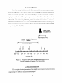
An experimental research program has been initiated to investigate the electrical
properties of swelling shales (shales that have been exposed to water and are therefore
expanding) across a wide frequency range, 5 Hz to 1.3 GHz. This range spans the spectrum
of the commonly used downhole logging measurements, from the deep laterologs to the
microwave dielectric tools. Three different methods of varying the sample's water content
have been used: desiccator, electro-osmosis and air exposure methods. Two distinct
measurement techniques have been used to span the frequency range: four-electrode setup
for the low frequencies (5 Hz -13 MHz), and open-ended coaxial probe with network
analyzer at the high end (20 MHz - 1,3 GHz), The probe technique is simple to use,
potentially enabling field measurements of complex permittivity to be taken, although some
accuracy is sacrificed. The effects of swelling in shale are most pronounced at the lowest
frequencies. This investigation discovered a phenomenon of shale; shale will generate a
direct electrical current under stress that has potential for a wellbore diagnostic tool. Also,
the best fluid for shale preservation was found to be Isopar M^^ (a mineral oil), saturated
with deionized water.
VI
LIST OF TABLES
4.1.
Salt Water Activity
29
4.2.
X-Ray Diffraction BuUc Analysis Results (Javalagi, 1990)
31
C.l.
Data Processing Programs / Scripts
127
vu
LIST OF FIGURES
2.1
Parallel - Plate Method
9
2.2
Two and Four Electrode Setup
9
2.3
Coaxial Method
10
2.4
Cavity Method (Blackham, 1990)
11
2.5
Open-Ended Probe
12
3.1
Silica Tetrahedron (Eslinger, 1988)
15
3.2
Octahedral Sheet (Eslinger, 1988)
15
3.3
Sketch of Kaolinite (Eslinger, 1988)
15
3.4
Sketch of Muscovite (Eslinger, 1988)
16
3.5
Schematic Diagram of the Structure of Kaolmite (Holtz and Kovacs, 1981)
17
3.6
Schematic Diagram of the Structure of Montmorillonite
(Holtz and Kovacs, 1981)
17
Diffuse Electric Double-layer According to Guoy-Chapman (Olphen, 1963)
Overlaid With Potential Distribution p
19
3.8
Potential Distribution of Stem's Electric Double Layer (Olphen, 1963)
20
3.9
Debye Circuit
24
4.1
Sample Casting
28
4.2
Quick Cut Sample Holder
28
4.3
Weight Change as a Function of Water Activity (Adisoemarta et al„ 1995)
30
4.4
Buoyancy Measurement Setup (Adisoemarta et al,, 1995)
33
4.5
Buoyancy Changes of Shale (Adisoemarta et al„ 1995)
33
4.6
Conductivity Changes After Shale Inunersion
35
4.7
Dielectric Constant of Confining Fluid
35
4.8
Dissipation Factor of Confining Fluid
36
4.9
Acoustic and Resistivity Measurement Setup
37
3.7
vni
4.10
Electrical and Computer Setup for the Acoustic
and Resistivity Measurement
38
4.11
Resistivity and Acoustic Travel Time as the Sample Is Drying Out
38
4.12
Sample Drying Conditions
39
5.1
Frequency Span of the Measurement Equipment and
Current Commercial Logging Tool Frequencies
41
5.2
Parallel-plate Measurement Technique
42
5.3
Open-ended Measurement
43
5.4
Complex Electrical Properties of Alcryn as a Function of Frequency
44
5.5
Effective Dielectric Constant of Deionized Water
45
5.6
Complex Electrical Properties of Methanol
46
5.7
Effective Conductivity of NaCl and KCl
47
5.8
Effective Conductivity of Pierre Shale as a Function of Water Content
48
5.9
Electro-osmosis Method
49
5.10
Electro-osmosis Current
50
5.11
Water Content and BHN versus Distance for Sample H
50
5.12
Water Content and BHN versus Distance for Sample I
51
5.13
Dielectric Constant of Sample H at Three Logging Frequencies
51
5.14
Dielectric Constant of Sample I at Three Logging Frequencies
52
5.15
Electrical Properties of Sample H at 20 kHz
53
5.16
Electrical Properties of Sample H at 2 MHz
53
5.17
Electrical Properties of Sample H at 1.1 GHz
54
5.18
Electrical Properties of Sample I at 20 kHz
55
5.19
Electrical Properties of Sample I at 2 MHz
55
5.20
5.21
5.22
Electrical Properties of Sample I at 1.1 GHz
Experiment Procedure Timeline
Relative Change of Conductivity at Various Frequencies
56
57
as a Function of Time in Inert Fluid
58
Changes in Weight as a Function of Air Exposure Time
59
5.23
ix
5.24
Sample Weight and Loss of Water in Place as a
Function of Cumulative Exposure Time
59
5.25
Error Bar Plot of a Shale Measurement
60
5.26
Variance Range of a Shale Measurement
60
5.27
Conductivity of WeUington Shales as a Function
of Frequency and Water Loss
Conductivity of WeUington WN1 at 35 Hz
as a Function of Water Loss
5.28
5.29
5.30
5.31
5.32
5.33
5.34
5.35
5.36
5.37
5.38
5.39
5.40
5.41
62
63
Conductivity of WeUington WN 1 at 280 Hz
as a Function of Water Loss
63
Conductivity of WeUington WNl at 20 kHz
as a Function of Water Loss
64
Conductivity of WeUington WNl at 10 MHz
as a Function of Water Loss
64
Conductivity of WeUington WNl at 250 MHz
as a Function of Water Loss
65
Conductivity of Wellington WNl at 1,1 GHz
as a Function of Water Loss
65
Dielectric Constant of WelUngton Shale as a
Function of Frequency and Water Loss
68
Dielectric Constant of WelUngton WNl at 35 Hz
as a Function of Water Loss
69
Dielectric Constant of WeUington WNl at 280 Hz
as a Function of Water Loss
69
Dielectric Constant of Wellington WNl at 20 kHz
as a Function of Water Loss
70
Dielectric Constant of WelUngton WNl at 10 MHz
as a Function of Water Loss
70
Dielectric Constant of WelUngton WNl at 250 MHz
as a Function of Water Loss
71
Dielectric Constant of WelUngton WNl at 1,1 GHz
as aFunction of Water Loss
71
Dissipation Factor of WelUngton as a Function
of Frequency and Water Loss
7^
x
5.42
Local Maxima and Minima of the Dissipation Factor of
Wellington WNl as a Function of Water Loss
73
Local Maxima and Minima of the Dissipation Factor of
Wellington WN2 as a Function of Water Loss
73
Local Maxima and Minima of the Dissipation Factor of
WeUington WN4 as a Function of Water Loss
74
Local Maxima and Minima of the Dissipation Factor of
Wellington WN5 as a Function of Water Loss
74
Dissipation Factor of Wellington WNl at 35 Hz
as a Function of Water Loss
75
Dissipation Factor of WelUngton WNl at 280 Hz
as a Function of Water Loss
75
Dissipation Factor of WelUngton WNl at 20 kHz
as a Function of Water Loss
76
Dissipation Factor of WelUngton WNl at 10 MHz
as a Function of Water Loss
76
Dissipation Factor of WelUngton WNl at 250 MHz
as aFunction of Water Loss
77
Dissipation Factor of WelUngton WNl at 1.1 GHz
as a Function of Water Loss
77
6.1
Schematic Diagram for Induced DC Measurement
78
6.3
Uiduced DC with Tune
79
6.2
Induced DC versus Load
79
6.4
Induced DC on Various Materials
80
6.5
Induced Polarization Decay Curve (Telford et al., 1990)
81
6.6
Induced DC on Small WeUington Shale
81
6.7
Induced DC on Big Wellington Shale
82
6.8
Shale and Ceramic Disc on Cyclic Loading
83
6.9
Voigt and MaxweU Viscoelastic Models
84
A, 1
Conductivity of Wellington WN2 at 35 Hz
as a Function of Water Loss
93
5.43
5.44
5.45
5.46
5.47
5.48
5.49
5.50
5.51
XI
A,2
A,3
A.4
A.5
A.6
A.7
A. 8
A.9
A. 10
A. 11
A. 12
A, 13
A, 14
A, 15
A, 16
A, 17
A, 18
A. 19
Conductivity of WeUington WN2 at 280 Hz
as a Function of Water Loss
93
Conductivity of Wellington WN2 at 20 kHz
as a Function of Water Loss
94
Conductivity of WeUington WN2 at 10 MHz
as a Function of Water Loss
94
Conductivity of WeUington WN2 at 250 MHz
as a Function of Water Loss
95
Conductivity of WeUmgton WN2 at 1.1 GHz
as aFunction of Water Loss
95
Dielectric Constant of WelUngton WN2 at 35 Hz
as a Function of Water Loss
96
Dielectric Constant of WelUngton WN2 at 280 Hz
as a Function of Water Loss
96
Dielectric Constant of WelUngton WN2 at 20 kHz
as aFunction of Water Loss
97
Dielectric Constant of WelUngton WN2 at 10 MHz
as a Function of Water Loss
97
Dielectric Constant of WelUngton WN2 at 250 MHz
as aFunction of Water Loss
98
Dielectric Constant of WelUngton WN2 at 1.1 GHz
as aFunction of Water Loss
98
Dissipation Factor of WelUngton WN2 at 35 Hz
as aFunction of Water Loss
99
Dissipation Factor of WelUngton WN2 at 280 Hz
as a Function of Water Loss
99
Dissipation Factor of WelUngton WN2 at 20 kHz
as aFunction of Water Loss
100
Dissipation Factor of WelUngton WN2 at 10 MHz
as a Function of Water Loss
100
Dissipation Factor of WelUngton WN2 at 250 MHz
as a Function of Water Loss
101
Dissipation Factor of WelUngton WN2 at 1,1 GHz
as aFunction of Water Loss
101
Conductivity of WeUington WN4 at 35 Hz
as aFunction of Water Loss
102
xu
A.20
A.21
A.22
A.23
A.24
A.25
A.26
A.27
A.28
A.29
A.30
A.31
A.32
A.33
A,34
A,35
A,36
A.37
Conductivity of WeUington WN4 at 280 Hz
as a Function of Water Loss
102
Conductivity of WeUington WN4 at 20 kHz
as aFunction of Water Loss
103
Conductivity of WeUington WN4 at 10 MHz
as aFunction of Water Loss
103
Conductivity of WeUington WN4 at 250 MHz
as aFunction of Water Loss
104
Conductivity of WeUmgton WN4 at 1.1 GHz
as aFunction of Water Loss
104
Dielectric Constant of WelUngton WN4 at 35 Hz
as a Function of Water Loss
105
Dielectric Constant of WelUngton WN4 at 280 Hz
as aFunction of Water Loss
105
Dielectric Constant of WelUngton WN4 at 20 kHz
as aFunction of Water Loss
106
Dielectric Constant of WelUngton WN4 at 10 MHz
as a Function of Water Loss
106
Dielectric Constant of WelUngton WN4 at 250 MHz
as a Function of Water Loss
107
Dielectric Constant of WelUngton WN4 at 1.1 GHz
as a Function of Water Loss
107
Dissipation Factor of WelUngton WN4 at 35 Hz
as a Function of Water Loss
108
Dissipation Factor of WelUngton WN4 at 280 Hz
as a Function of Water Loss
108
Dissipation Factor of WelUngton WN4 at 20 kHz
as a Function of Water Loss
109
Dissipation Factor of Wellington WN4 at 10 MHz
as a Function of Water Loss
109
Dissipation Factor of WelUngton WN4 at 250 MHz
as a Function of Water Loss
110
Dissipation Factor of Wellington WN4 at 1,1 GHz
as aFunction of Water Loss
HO
Conductivity of Wellington WN5 at 35 Hz
as aFunction of Water Loss
HI
xiu
A.38
A.39
A.40
A.41
A.42
A.43
A.44
A.45
A.46
A.47
A.48
A.49
A.50
A.51
A.52
A,53
A,54
Conductivity of WeUington WN5 at 280 Hz
as a Function of Water Loss
Ill
Conductivity of WeUington WN5 at 20 kHz
as aFunction of Water Loss
112
Conductivity of WeUington WN5 at 10 MHz
as aFunction of Water Loss
112
Conductivity of WeUington WN5 at 250 MHz
as aFunction of Water Loss
113
Conductivity of Wellington WN5 at 1.1 GHz
as aFunction of Water Loss
113
Dielectric Constant of Wellington WN5 at 35 Hz
as aFunction of Water Loss
114
Dielectric Constant of WelUngton WN5 at 280 Hz
as aFunction of Water Loss
114
Dielectric Constant of Wellington WN5 at 20 kHz
as aFunction of Water Loss
115
Dielectric Constant of WelUngton WN5 at 10 MHz
as a Function of Water Loss
115
Dielectric Constant of Wellington WN5 at 250 MHz
as aFunction of Water Loss
116
Dielectric Constant of WelUngton WN5 at 1.1 GHz
as a Function of Water Loss
116
Dissipation Factor of WelUngton WN5 at 35 Hz
as aFunction of Water Loss
117
Dissipation Factor of WelUngton WN5 at 280 Hz
as a Function of Water Loss
117
Dissipation Factor of WelUngton WN5 at 20 kHz
as aFunction of Water Loss
118
Dissipation Factor of WelUngton WN5 at 10 MHz
as a Function of Water Loss
118
Dissipation Factor of WelUngton WN5 at 250 MHz
as a Function of Water Loss
11^
Dissipation Factor of WelUngton WN5 at 1.1 GHz
as aFunction of Water Loss
H^
CI
Program Listing of IMP.BAS
1-8
C.2
Program Listing of lA-MULTLBAS
138
XIV
C,3
Program Listing of lA-MULTLBAS
146
C.4
Program Listing of NA-MULTI.BAS
150
C.5
Program Listing of IANAMRG3.BAS
153
C.6
Program Listing of WN3dPLOT.M
156
C.7
Program Listing of LOGFPLOT.M
158
C.8
Program Listing of DAS.BAS
160
C.9
Program Listing of BALANCE.BAS
171
XV
CHAPTER I
FORMULATION OF THE PROBLEM
1.1 Introduction (Adisnemarfa and Morriss IQQ?^
Anomalously low resistivity-log response in certain formations has been known to
yield incorrect water saturation and to sometimes mask detection of hydrocarbon-bearing
intervals. Shale, which is often the cause of the problem because of its clay content, may
be in the form of laminations or grains, both detrital in origin. The interpretation problem
is one of choosing the appropriate mixing mle based on both the distribution of the shale
and the volume investigated by the logging measurement. An understanding of the electrical properties of the shale itself is an important element of the problem. For example, complex permittivity can be used in a model based on a volumetrically weighted mixing mle to
interpret microwave-frequency measurements. In a shaly formation, these complex-time
average models require values for the complex permittivity of the shale. High resolution
dielectric logging measurements may be able to detect individual shale laminae if they are
thick enough, in which case the shale's properties must be accounted for in the interpretation.
The electrical properties of massive shales are also of interest to the industry. The
alteration of shales, caused by adsorption of water while drUUng, is one of many contributors to the wellbore stability problem that costs the industry in the order of $ 400 -500 million annuaUy (Bol et al,, 1992). This alteration of shale problem has acquired a logging
perspective due to the increasing use of measurements while drilUng. The capabiUty of taking real time and time-lapse measurements whUe stiU driUing introduces the possibUity of
detecting a swelUng problem while something can stUl be done about it.
Improved interpretation in both of these cases requires an understanding of the effect of the shale's composition, texture, chemistry, and water content on tool response. In
particular, the effect on electrical measurements can be quite large. The avaUability of tools
operating over a wide range of frequencies is of possible benefit since the mechanisms
affecting the propagation of an electromagnetic wave differ with frequencies. Logging
measurements at frequencies from 35 Hz to 1.1 GHz are conunerciaUy avaUable.
It is conunon to speak of conductivity and electrical permittivity as the material
properties affecting electromagnetic wave propagation. (Magnetic permeabUity is usually
negligible in sedimentary formations.) These two properties are distinguished by the phase
relation between stimulus and response, from a measurements point of view, with the conductivity being associated with the in-phase response and the permittivity with the quadrature response. The corresponding physical mechanisms are electronic or ionic movement
for conductivity and various polarization mechanisms for permittivity. However, in a material as complex as a clay-bearing rock, this model is too simpUstic since most mechanisms
exhibit a frequency-dependent phase and amplitude response. For example, at very high
frequencies, ionic conduction wUl not be able to stay in phase with tiie stimulus, just as
electron conduction fails to stay in phase at optical frequencies. Mathematically, this generalization can be handled by representing both conductivity and permittivity as complex
numbers. There are thus four electrical properties characterizing a clay-bearing rock.
Since water in the pore spaces and adsorbed to the mineral surfaces is a major influence on the electrical properties of a shale, this paper investigates the effect of changing
the amount of bound water adsorbed to the clays. Shale samples with different clay compositions are placed sequentially in desiccators, each of which contains a different saturated
saU solution that creates a known water activity The shale is brought to equiUbrium at each
step, and the electrical properties are measured. Weight changes from the known initial
state indicate the amount of water gained or lost. Using the known CEC, the surface area
of the clays and the average thickness of the water can be estimated. Two other methods of
adjusting the water saturation in the sample have also been implemented, which are the
electroosmosis method and the air-drying method. Under tiie electroosmosis method, the
sample is a long core sample that is impressed with a direct current for a period of time, and
after that cut into thin slices. The air-drying method exposes the sample to ambient air under a controlled condition; thus the remaining pore water can be determined. Then, after a
period of equilibration, the sample is measured for its electromagnetic properties.
Preservation fluid is also studied thoroughly, as this fluid is very important in preserving the condition of the sample either for short-term or long-term storage. Movement
of pore water into or out of the sample is determined by changes in sample weight and
changes in electromagnetic properties of the preservation fluid.
This dissertation is a continuation of the author's graduate research that has been
previously reported on his Master's report (Adisoemarta, 1995); as such there wiU be several discussions referring back to that document.
1.2 Report Systematics
This report will be arranged as foUows: Chapter I wiU present the problem statement; Chapter II will give the theoretical background of electromagnetic properties and
measmrements; some studies that have been done in the past wiU be presented in Chapter
III, followed by the sample preparation techniques in Chapter IV; electromagnetic measurements results are described in Chapter V; the induced DC potential phenomena in Chapter
VI; and Chapter VII will present the conclusions.
CHAPTER n
IMPEDANCE EM POROUS MEDIA
2,1 Shale Conductivity Theory
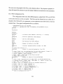
The macroscopic electrical behavior of conducting dielectrics subjected to a harmonic sinusoidal field is described by MaxweU's equations and certain constitutive relationships.
All electromagnetic fields are created from distributions of charges and currents in
which the electric field (resulting from the charge distributions), and the current densities
(from the current distributions) are related through the complex transfer functions that result from Maxwell's equations:
V*E + dB/dt
= 0
V*H - dD/dt -J = 0
(2.1)
(2.2)
and with the conservation of charge defined as:
^•J-dq/dt=0
(2.3)
are the five components of the electromagnetic field, where:
E = electric field intensity (volt/meter)
B = magnetic flux density (webers/meter^)
H = magnetic field intensity (ampere-tum/meter)
D = electric displacement (coulomb/meter^)
J
= electric current density (ampere/meter )
q
= charge density (coulomb/meter ).
For the case of homogeneous, isotropic, and a non-zero electrical conductivity medium,
the electric field becomes
V«£ = 0 ,
(2.4)
For the case of materials that exhibit electromagnetically linear behavior, the following relationships are vaUd:
D =
EE
(2.5)
J = cE
(2.6)
B = \iH
(2.7)
where
8 = dielectric permittivity (farad/m)
a = electric conductivity (mho/m or siemens/m)
jLi = magnetic permeabUity (henry/m).
The equation for total current density, J^ , is the result of solving equations (2,2),
(2.5), and (2,6):
J J = V*H = (5E + edE/dt
(2,8)
where GE is the conduction current component (in phase with applied voltage), and
edE/dt is the displacement current component (the out of phase response).
For the time-harmonic case, in which temporal behavior, Ej, , described by
E^ = E ^ . - - ' " '
(2.9)
where
;•
=(-1)''^
OD = frequency (radians / sec),
the total current density 7 ^ in a medium becomes the following:
J^ = {0^-j(DE*)Ej
(2.10)
where a* and £* are, in general, complex scalars dependent upon frequency (Fuller and
Ward, 1970).
By substituting these complex scalars, with thek respective real (shown with a single prime,' ) and imaginary (shown with a double prime,") components,
a* = &-j&'
(2.11)
£* = £ ' - ; 8 "
(2.12)
equation (2.10) can be rewritten as the following:
^T " ^^eff'-^^^efp^T
(2-13)
where (j^-^ = c' + coe" and E^^ = e' - a"/03 are real functions of frequency that constitute
the experimentally measured rock parameters (FuUer and Ward, 1970).
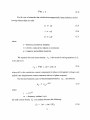
In the simplest form, equation (2.13) becomes the famiUar Ohm's law that relates
electric current to the voltage across the medium and the conductance of the medium itself.
Ohm's law is as follows:
I = GV
(2.14)
where
I = electric current (amperes)
G = electric conductance (mho or Siemens)
V = electric potential (volt).
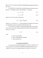
7 ? rnndiTctivitv and Susceptivitv
The output from the measurement equipments are not dUectiy comparable to each
other, and they have to be converted to conductivity and susceptivity before they can be
compared to each other. For the impedance analyzer, the outputs are resistance and
reactance. The conversions to resistivity, reactivity, conductivity and susceptivity are calculated using the equations below:
Rnd^
f
/
(2.15)
t
Xnd^
"V*
X
Ct
—
8
b
(2.16)
t
=^
r
2, 2
r +X
—X
2,
2
r -\-X
(2,17)
(2.18)
where
R = resistance (ohm)
X = reactance (ohm)
r
= resistivity (ohmmeter)
X = reactivity (ohmmeter)
t
= sample thickness (meter)
d
= electrode diameter (meter)
g
= conductivity(Siemens/meter)
b
= susceptivity (Siemens/meter).
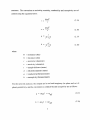
For the network analyzer, the outputs are in real and imaginary (in-phase and out-ofphase) permittivity, and the conversions to conductivity and susceptivity are as follows:
g = coe.e" = o^^f
(2.19)
b = 0)8,8' = C08^^^
(2.20)
where
g
- conductivity (Siemens/meter)
b
= susceptivity (Siemens/meter)
8' = relative permittivity, real part (dimensionless)
8" = relative permittivity, imaginary part (dimensionless)
80 =8.854xl0"^2(paj-ads/meter).
2.3 Dissipation Factor
A dielectric parameter that wiU be used in this research is the dissipation factor. The
dissipation factor is defined as the ratio of in-phase to quadrature current components:
8"
D = ^
.
(2.21)
2 4 Dimensionless Properties
Two dimensionless properties that wiU be used in this report are the dimensionless
forms of effective conductivity and effective permittivity.
The dimensionless effective conductivity is
a ..
= —^
.
(2.22)
The dimensionless form of effective permittivity is
£
e
eff
= —^
8
P 23)
2.5 Rlectromafmetic Measurement Terhnign^Q
There are several methods in the frequency-domain for measuring electromagnetic
properties of materials, and the most popular methods are described herein.
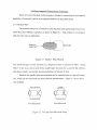
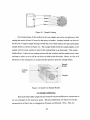
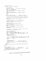
2.5.1 Parallel-Plate
The material under test is formed as a thin flat sheet and sandwiched between two
electrodes, thus making a capacitor, as shown in Figure 2.1. This metiiod is very dependable and very easy to implement.
Material
under test
Electrodes
Figure 2.1 Parallel - Plate Method
The disadvantages of this method are a frequency limit of around 15 MHz; "fringe
effect" or the stray current path at the sample edge; necessity for a smooth, flat with paraUel faces sample; and sample maximum thickness of around 10 mm.
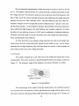
Methods for parallel-plate measurement can be separated into two general categories, which are two-electrode and four-electrode measurements. Figiue 2.2 shows these
two methods.
Voltage Electrodes
Voltage
JC
IN
Current Electrodes
Current Electrodes
Two-Electrode
Four-Electrode
Figure 2.2 Two and Four Electrode Setup
The two-electrode measurement is where the set-up is exacdy as shown in the Figure 2.1. The sample is placed between two current electrodes, and these electrodes are also
the voltage electrode. This method is prone to errors at the lower end of the frequency, less
than 10 kHz, due to the contact impedance from the ionic buUd-up at the sample-electrode
interface (Lewis et al., 1986; Garrouch, 1992). The ionic build-up is the zone where the
frequency changes are slow enough that ions have sufficient time to "pile up" at the sample-electrode interface. As the frequency increases, the possibiUty of buUd-up diminishes,
and at sufficiently high frequency, the ionic buUd-up zone varushes completely. To reduce
the effect of ionic build-up, Scott et al. (1967) used a combination of platinized platinum
electrodes and blotter pads to increase the surface area at the sample-electrode interface,
hence minimizing the ionic build-up.
In a foiu:-electrode set-up, separate voltage electrodes are used at each sample face
located away from the current electrodes, outside the ionic build-up zone. As the voltage
electrodes have a high impedance, they will draw almost no ciurent, so that essentially no
ionic build-up will occur at the voltage electrodes.
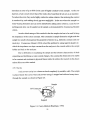
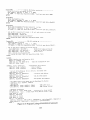
2.5.2 Coaxial
The sample is shaped into a core with a hole in the middle and inserted into a short
coaxial airline. The center conductor is passed through the hole in the sample, as shown in
Figiue 2.3. The frequency range of this method is very broad, 100 MHz to 18 GHz.
Sample
Center Conductor
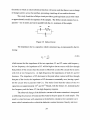
Figure 2.3 Coaxial Method
The disadvantage of this method is that tiie sample needs to be carefully machined
to avoid error due to the presence of an air gap between the sample and the airline wall or
the center conductor. Huang and Shen (1983) found that even air gaps of 10"^ inches can
10
introduce an error of up to 60% for the case of highly conductive rock samples. As the conductivity of air is much lower than of the rocks, they found that the air acts as an insulator.
To reduce the error, they used a highly conductive saline solution, thus reducing the contrast
in conductivity, and making the air gap error negligible. In the case where the sample is a
water-bearing formation and can not be disturbed by adding saline solution, a coat of a low
melting point alloy can be appUed on the sample, as demonstrated by Coutanceau-Monteil
(1993).
Another disadvantage of this method is that the sample size has to be smaU to keep
the impedance of the system constant. This constraint in sample dimension might make the
sample too small to homogenize the parameter of interest (e.g., dielectric constant, and conductivity). Coutanceau-MonteU (1993) solved this problem by using tapered adapters in
which the impedance was kept constant from the analyzer to the coaxial cable to the sample
holder and back to the analyzer.
Due to difficulties in machining the sample and the inherent characteristic of shale
expanding and shrinking as water content changes, thus causing the dimension to be unable
to be constant and mamtain its physical fitness inside tiie airline, tiie research in this dissertation did not use this method.
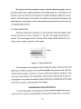
2.5.3 Cavity
A microwave cavity is a volume enclosed completely by metaUic waUs. The sample
is placed inside this cavky where microwave energy is trapped and reflected many times
through the sample, as shown in Figure 2.4.
Sample
RF Connector
Support
Figure 2.4 Cavity Method (Blackham, 1990)
11
The change in the electromagnetic response with and without the sample in the cavity is then related to the complex permittivity of the sample-under-test. This method is very
sensitive to low-loss dielectrics and requires less sample machining compared to coaxial
method. The disadvantage of this method is this method is not broad-band in frequency but
single frequency measurement, which is determined by the physical size of the cavity, and
is computationally intensive
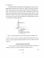
2.5.4 Open-Ended Probe
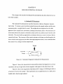
The open-ended probe is basically a cut-off coaxial line where the sample touches
the face of the probe, as shown in Figure 2.5. The face of the sample must be flat and
smooth. The electromagnetic field is reflected off the sample, and the reflection (S^) is
related to the complex permittivity of the sample.
Sample
W!^^^^^^^^^^^MW
Probe
Figure 2,5 Open-Ended Probe
The advantages of this method are tiiat the frequency range is relatively broad (100
MHz up to 2.6 GHz), the probe is very small and portable, tiie probe can work with both
solid and liquid samples, and there is no need to machine tiie sample for a perfect fit, such
as for the coaxial-method. The disadvantage of this metiiod is that because the depth-ofinvestigation is very small, the reading is mostiy affected by a small portion of tiie sample
and is thus very prone to heterogeneity of the sample,
9 f^ MethoHolnpv Tked in This Research
To ensure the quality of measurements, the four-electrode parallel-plate setup is
used for the low frequency electromagnetic measurements. Fringe effect is reduced by
12
using the thinnest sample disks as possible. The Open-Ended probe method is used for
the high frequency electromagnetic measurements, as this method is very handy and has
fairly broad frequency coverage.
13
CHAPTER III
CONDUCTIVITY IN POROUS MEDL\
This chapter will cover clay minerals and their double layer properties and wiU
summarize several studies that have been done on tiie complex dielectric parameters of porous media.
3.1 Clav Minerals
The definition of clay evolve with time, as mention by Guggenheim and Martin
(1995), starting from 1546 up to the most recent definition jointiy pubUshed by the AIPEA
(Intemational Association for the Study of Clays) and the CMS (Clay Minerals Society),
The most recent definition (Guggenheim and Martin, 1996) is as foUows:
The term 'clay' refers to a naturally occuring material composed
primarily of fine-grained minerals, which is generally plastic at appropriate water contents and wiU harden when dried or fired. Although clay usuaUy contains phyllosUicates, it may contain other
materials that impart plasticity and harden when dried or fired. Associated phases in clay may include materials that do not impart
plasticity and organic matter. (p. 715 )
Clay minerals are only observable under an electron microscope. The individual
clay crystals are shaped like plates made of sheets of repeating atomic stmcture. FundamentaUy, the crystal sheets can be seen as only having two types, the tetrahedral or octahedral sheets. Different clay minerals are built from these two stmcture sheets with various
ways of stacking, together with various bonding and different metaUic ions in the crystal
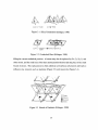
lattice. Figure 3.1 illustrates the components of a tetrahedral sheet, first consisting of silica
tetrahedron units with each unit made of one sUicon atom surrounded by four oxygen atom
(Figure 3.1 .a). These units are joined together to make a hexagonal network (Figure 3.1 ,b).
The octahedral sheet, as shown in Figure 3,2, is a combination of octahedral units
(Figure 3,2,a) that consist of six hydroxyls, surroundmg an aluminium, magnesium, or iron
atom, joined together to create a sheet (Figure 3,2,b),
In the tetrahedral sheet, Si^"*" is sometimes partially replaced by trivalent Ar"^. In
the octahedral sheet, trivalent Ap"^ can be replaced with divalent Mg^"^ without completely
14
(al
Q
Ibl
and ;'^i » Oxygens
Q and 0
= Silicons
Figure 3.1 SUica Tetrahedron (Eslinger, 1988)
• (a)
Q
and '^^ = Hydroxyls or
oxygens
I Aluminums, magnesiums, etc.
Figure 3.2 Octahedral Sheet (Eslinger, 1988)
filUng the vacant octahedral position. Al atoms may also be replaced by Fe, Cr, Zn, Li and
other atoms, and the small size of the these atoms permits them to take the place of the small
Si and Al atoms. This replacement is often called an isomorphous substitution and leads to
different clay minerals such as kaolinite (Figiue 3.3) and muscovite (Figiue 3.4).
(~)
Oxygens
6 H ) Hydroxyls
^P
9
Aluminums
OSilicons
Figure 3.3 Sketch of Kaolinite (EsUnger, 1988)
15
In many minerals, an atom of lower positive valence replaces one of higher valence,
creating a deficit of positive charge and therefore an excess of negative charge. This excess
of negative charge is compensated by the adsorption on the layer surfaces of cations, which
are too large to be accommodated in the interior of the lattice. In the presence of water, the
compensating cations on the layer surfaces may be easily exchanged by other cations when
avaUable in solution; they are caUed exchangeable cations. Analytical methods can determine the amount of these cations. This amount, expressed in miUiequivalents per 100
grams of dry clay, is called the cation exchange capacity (CEC).
n H , 0 layers and exchangeable cations
Q
Oxygens
@
Hydroxyls
0
Aluminum, iron, magnesium
O and # Silicon, occasionally aluminum
Figure 3,4 Sketch of Muscovite (Eslinger, 1988)
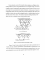
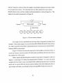
Figures 3.5 and 3.6 show a method to make the sheet in the clay minerals easier to
visuaUze, by using "schematic representation" oftiietetrahedral or octahedral sheets. Figure 3.6 also shows arrows that point to the inter-layer gap on montmorillonite where water
and exchangeable ions can enter and separate the layers that are held together by weak
16
bonding (van der Waal's bonding) between the tops of the siUca sheets, and the net negative
charge deficiency in the octahedral sheet.
The inter-layer, also caUed intra-crystaUine, swelUng that occurs after montmorillonite clays are contacted with water or water vapor, wiU generate more or less stable configuration of the hydrated clay, corresponding to the presence of one to four monomolecular
layers of water between the unit layers.
Al
\
Al
Zi
\."-"'
Al
zcr
Si
\
Figure 3.5 Schematic Diagram of the Stmcture of Kaolinite (Holtz and Kovacs, 1981)
nHjO layers and
exchangeable cations
0.96 nm
Figure 3.6 Schematic Diagram of tiie Stmcture of MontmoriUonite
(Holtz and Kovacs, 1981)
17
3.2 Rleotrin n o n h i e Layer
The preceding section shows that, as a result of isomorphous substitutions by elements of lower valence, the clay lattice carries a net negative charge. The net negative lattice charge is compensated by cations that are located on the unit-layer surface. The cations
diffuse m the presence of water, as their concentration wUl be smaUer in the buUc solution.
But, due to the charged lattice, these cations wUl also be attracted electrostatically, and the
resuk of these opposing trends is the creation of a distribution of compensating cations in
a diffuse electrical double layer on the exterior layer surfaces of a clay particle, Olphen
(1963) mentioned that this distribution of charge is analogous to that in the earth's atmosphere where the gas molecules are both attracted to the earth by gravitation and diffusion
to the outer space. There are two models that are commonly used to explain the double layer, the Gouy-Chapman Model and Stem Model.
3.2.1 The Gouy-Chapman Model
An electric double layer consists of a surface charge and a compensating counterion charge that creates a "cloud" of ions with a diminishing concentration away from the
charged surface (Figure 3.7). This model assumes that the ions in the fluid are point charges, the fluid is a continuous medium, and only the dielectric constant properties of the fluid
affects the double layer. From the electrostatic and diffusion (Poisson-Boltzmann) theory,
the exact distribution of positive and negative ions can be determined as a function of distance from the surface. The net charge concentration distribution, p , for any position from
a positively charged surface can be derived as a function of the potential ^ :
ze"^
p = ze{n^+n)
= -2nzeS\nh-—
where
Uo
= ion concentrations in the bulk electrolyte
n+
= ion concentrations of the positive ions
n.
= ion concentrations of the negative ions
T
= temperature
k
= Boltzman constant
18
(3.24)
z
= ion valence
e
= electron charge.
The potential, "¥, away from the surface can be solved by utiUzing the Poisson equation,
and ends up as the Poisson-Boltzmann equation:
^Kn ze
sinh
ze^
~kT
(3.25)
with D as the dielectric constant of the medium. This net charge in the diffuse layer
should be equal to the charge on the surface to satisfy the electroneutrality:
o = -\ze{n^-n_)dx
(3 26)
where surface charge density on the siuface is denoted as a.
PARTICLE
SOLUTION
P+=P-=P
Figure 3.7 Diffuse Electric Double-layer According to Guoy-Chapman (Olphen, 1963)
Overlaid With Potential Distribution p
The Gouy-Chapman model of the electric double layer contains some unrealistic elements, such as ions treated as point charges and neglect of thefiiutedimensions of the
ions. Also, the specific interactions between the surface, counter-ions and medium are ignored. These assumptions are tolerable in dilute solutions where the diffuse layer is wide,
but in concentrated electrolytes, this model fails.
19
3.2.2 Stem Model
This model considers that the distance of closest approach of a counter-ion to the
charged surface is limited by the size of these ions. Figure 3.8 shows that the counter-ion
charge is separated from the surface charge by a layer of thickness 6 in which there is no
charge. This setup basically creates an electric condenser of molecular size, formed by the
surface charge and the charge in the place of the centers of the closest counter-ions. In this
condenser, also called the "Stem layer," the electric potential drops Unearly with distance
from a value OQ at the surface to the Stem potential, O5. The remaining part is distributed
as in a diffuse Gouy-Chapman atmosphere.
- S T E R N LAYER
(MOLECULAR CONDENSER)
oa.
POSITION
OF
STERN lONS-^
DISTANCE FROM SURFACE
•(J : SURFACE POTENTIAL
• j -. STERN POTENTIAL
er, : NET COUNTER-ION CHARGE OF STERN LAYER
a- • NET COUNTER-ION CHARGE OF DIFFUSE LAYER
2'
IT . TOTAL CHARGE ' V^ •*• a^
Figure 3.8 Potential Distribution of Stem's Electric Double Layer (Olphen, 1963)
The total counter-ion charge in this model is split between the charge inside the condenser (Ci) and the charge in the difftise atmosphere (02); the sum is equal to tiie surface
charge (a).
^ ^ Dielectric MnHels of Clavev Media
The most widely used fomiula, and also the sunplest to describe the electrical conductivity on porous rock, is Archie's law, defined in conductivity form as
CJo = ^ w a (j)m
20
(3.27)
where
CQ
= electrical conductivity of fully fluid saturated rock
Gvv
= electrical conductivity of saturating fluid
())
= pore volume fraction
a
= empirical parameter
m
= empirical parameter (cementation factor)
and formation factor, F, is defined as the ratio of Gy^/a^.
For the case of a partially water saturated condition. Equation (3,4) becomes
G
t
^.n
S'
w G
w
(3.28)
^ '
where
Gx
= electrical conductivity of partiaUy saturated rock
S^
= fractional water saturation
n
= saturation exponent.
Archie's model assumes that electrical conduction through the saturating fluids in
the pores is the dominant factor, and surface conduction along pore waUs is negUgible. This
model would faU in porous media that has even a smaU amount of clay in the pores, as surface conduction due to cation exchange would be a significant factor. However, the magnitude of the surface conductance effect is also a function of salinity of the pore water and
the CEC of the clay minerals. Several models that have been proposed to modify Archie's
model to include the clay effect wUl be discussed herein.
3.3,1 Waxman-Smit (1968)
The modification of Archie's model with the extra surface conduction and cation
exchange capacity in shale and clay-bearing sands results m the foUowing equation:
Go = (Ow + BQv) a ({)°^
(3.29)
ao = [l/F](a^ + BQv)
(3.30)
or
21
where
B
= equivalent conductance of counter-ions associated with clay in pore water,
determined empiricaUy as
B = 4.6(1-0,6 e"^-^'77aw)
Qv = cation exchange capacity per unit pore volume.
For a partial water saturated pore condition. Equation 3.6 becomes
at = (a^S^° + BQ^S^P) a G^
(3.31)
where
p
= clay content as a fraction of tiie buUc volume.
3.3.2 Dual-Water (Clavier et al„ 1977)
This model enhances the Waxman-Smit model by assigning a specific "volume" to
the clay contributed conductivity in addition to the clay-free water conductivity. Hence this
model is called the "Dual-Water" (DW) model, as there are two water types that are being
predicted by the model, both for its conductivity and its volume fraction.
The first water is the clay water, which surrounds the clay particles. Its conductivity, GQ^, comes from the clay counterions. The volume fraction, V^w, is directly proportional to the counterion concentration, Qy
Vcw=VQQv(l)t
(3.32)
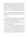
where
VQ = the amount of clay water associated with 1 unit (meq) of clay counterions
(j)t = total porosity.
The other water is the far water, the water that is farther away from the clay. This
water has conductivity, a^, and ionic concentration that corresponds to the salinity of bulkformation water. The volume fraction of free water, Vf^, is the remainder of the total water
content subtracted by the clay water
22
Vfw = Vw - Vcw = (S^T - VQ Qv ) (t)t.
(3.33)
The equivalent fluid conductivity of tiie formation is the combination of these two
fluids using the volumetric weighted averaging method:
C^we = { (SwT - V Q Qv ) a ^ + VQ QV G^^ } / S^j.
(3.34)
The partially saturated conductivity wiU be as foUows:
G. =
t
' wT
- ^
F
V G
G + - ^ ( a
-G )
w
S
cw w-^
(3,35)
3.3.3 Lima and Sharma (1992)
This model assumes that clays are charged particles siurounded by a counterion
double layer in which the polarization occius. This model has two sub-models with differing assumption on the polarization of the double layer. The first one is the S-model where
a Stem layer is included, but radial fluxes are assumed to be small. The second model is
the D-model, which assumes that only the diffuse layer polarizes. Comparison with experimental data showed that the S-model is suitable for cases in which most of the counterions
are tightly bound to the solid particles, but any ionic diffusion will make the prediction of
conductivity and permittivity higher than the actual observed values. The D-model is more
appropriate for representing the dielectric behavior of clay bearing rocks in the range from
1 to lO'^ Hz.
3.3.4 Knight and Nur (1984)
This study used a variety of sandstones representing a range in porosity from 6% to
28%, in permeabUity from microdarcies to miUidarcies, and in clay content from 0% to
18%. The dielectric constants of these sandstones were measured across the frequency
range of 5 Hz to 13 MHz as a function of water saturation and pore fluid saUnity,
The measurement electrodes consisted of a lOOOA thick platinum layer sputtered
onto the two flat faces of each disc-shaped sample. This technique makes a reversible
23
electrode in which an electrochemical reaction wiU occur such that there is an exchange
of charge carriers across the interface, preventing a buUd-up of ions and/or electrons.
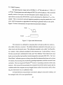
This study found that a Debye circuit provides a good equivalent circuit with which
to approxunately model the response of the samples. The Debye circuit contains two capacitors - one in series and one in paraUel with tiie d.c. resistance of tiie sample.
C2
R2
HI—V\An
f01
Figure 3.9 Debye Circuit
The impedance due to a capacitor, which is reactance (Xs), is represented by the following:
Y zz - L
^s
(oC
(3.36)
which means that the impedance of the two capacitors, CI and C2 varies with frequency.
At low frequency, the impedance of CI will be high so that no current will flow through
that portion of the circuit; thus the circuit is effectively a series RC circuit (R2 in series
with C2) at low frequencies. At high frequency, the impedances of both CI and C2
decrease. The impedance of C2 decreases to the point where current will flow through
that part of the circuit; the impedance of C2 decreases to essentially zero, leaving a parallel RC circuit (R2 in parallel with CI). The study found that the values of the two
capacitors are approximately 10'^ and 10'^^ Farads, with the former, CI, dominating the
low frequency and the latter, C2, the high frequency response.
The observed change of the dielectric constant with water saturation is interpreted
as reflecting the presence of bound and free water in the pore space of a rock sample. The
result is a rapid increase with saturation in the dielectric constant at low saturation up to
some critical saturation above which the dielectric constant increases linearly and more
24
gradually with saturation. The critical saturation is interpreted as reflecting tiie percentage
of bound water in the rock and is thus proportional to the surface-to-volume ratio of tiie
pore space.
3.3.5 Garrouch (1992)
This dissertation studies the effects of wettabUity, clay content, water samration and
salinity on the electrical properties of hydrocarbon-bearing rocks. The frequency range of
interest is 10 Hz to 10 MHz. Measurements were made for the impedance of both fully and
partiaUy saturated rocks using the four-electrode method for the latter, and the two-electrode method for the former. These measurements include both clean and shaly sand samples.
For fully saturated rocks, this study found that the dielectric constant increases with
the clay volume fraction, the cation exchange capacity, and the electrochemical potential of
the fluid saturating the rock samples. It is found to decrease with increasing saUnity, frequency, permeability, and porosity. Neither stress nor wettabUity appear to significantiy influence the dielectric constant of fuUy brine-saturated Berea cores.
The study has also inverted the Lima-Sharma theory for modelUng the complex impedance of partially saturated shaly sands. This inversion aUows a log analyst to use low
frequency (less than 1 KHz) and high frequency (higher than 1 MHz) complex impedance
data from well logs to calculate in-situ reservoir petrophysical parameters such as water saturations in the virgin formation and in the flushed zone, porosity, clay volume fraction, clay
surface charge density, and grain size. The resuk of the inversion method was implemented
using real well log input, resulting in a reasonably good output of reconstmcted log. The
sUght discrepancy between the actual values and the output model values are possibly due
to the finite difference method solution.
25
CHAPTER W
SAMPLE PREPARATION AND PRESERVATION
This chapter will describe the sample preparation includmg sample dimension requirements, cutting procedures, preconditioning, and preservation stages.
41 Sample Dimension Requirements
The main requirement for the sample dimension is to be able to use the same shale
sample on both parallel-plate and open-ended coaxial probe setups.
Diameter. The sample diameter has to be around the 2 inch (5.08 cm.) diameter of
the parallel-plate electrodes. This sample diameter also fits the requirement for the
open-ended coaxial probe, as it requires a sample diameter greater than 2 cm. (HP, 1993).
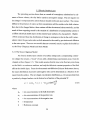
Thickness. The maximum sample thickness is determined by the parallel-plate setup, which is around 10 mm, and the minimum thickness is determined by the open-ended
probe specification. The depth of investigation of the open-ended coaxial probe is a function of the sample's relative permittivity and defined as the foUowing equation (HP, 1993):
d\mm)
—
^20 ^
^^ '
v^^y
(4.1)
where
d = minimum thickness (mm)
e^ = dielectric constant.
A low dielectric constant sample will be the worst case scenario for the open-ended
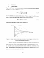
probe as the depth of investigation wiU be the deepest. Assuming that the lowest dielectric constant of the sample is 6, for a typical dry sandstone sample, then the depth of
investigation is around 8,2 mm. Hence the sample thickness has to be between 8.2 and
10 mm. For the case of 10 mm sample thickness. Equation 4.1 indicates that the lower
bound dielectric constant that can be measured is 4.
26
Parallel sample faces are very important for the parallel plate setup, as the sample
is the capacitive medium between the electrodes, and any deviation from a perfect parallel
sample makes the result questionable.
Sample flatness is another parameter that has to be defined carefully, as it determines the contact condition for both the parallel-plate setup and the open-ended coaxial
probe to the sample. A bad sample-electrode contact wiU put an air gap in between the sample surface and the electrode, and create an "air-gap error." The severity of such error has
been discussed in the past (Rau, 1980; Huang and Shen, 1983; Knight, 1984). The
open-ended coaxial probe requires samples to have flatness of less than 25 pm.
After combining the above requirements, the sample specification is as foUows:
sample surface flatness within 0.001 in (25 pm), parallel sample surfaces within 0.005 in,
and a sample thickness between 8-10 mm. The sample diameter is 2 in (5.08 cm).
4.2 Sample Preparation
The typical sample cutting method, using a clamp on a bench top saw, rarely gives
a good sample cut as the comer of the cut usually nicks when the undamped part falls off
from the main body near the end of the slicing process. This method is also prone to bad
parallelness as the manual handling of the core can not maintain the same orientation with
respect to the saw blade. Typically it takes a couple of days of manual sample sanding and
face lapping to bring those kind of samples to the required specification; thus the typical
sample cutting method is very time consuming and labor intensive. To avoid that kind of
problem and to ensure a good sample surface after each cutting, a technique of casting the
sample in an acrylic tube has been used. Figure 4.1 shows that the sample is held tightly
inside the clear acrylic tube by three (3) plastic rods that act as spacers, and the gap is then
filled with epoxy. This method wiU guarantee a smooth and parallel sample surface, as the
sample wUl not wobble and/or rotate while being cut, and also wiU not break unevenly at
the edge when the small piece of the sample breaks off. Even with this technique, a small
amount of time for sample face lapping is stiU needed to meet the required specifications.
This sample casting method cuts the sample preparation time from several days to about
one hour.
27
Figure 4.1 Sample Casting
One disadvantage of this method is the core sample can not be cut right away after
casting but needs at least 14 hours for the epoxy to harden. Another method was devised
for the case of urgent sample slicing in which the core is held inside a two-piece plexyglass
sample holder as shown in Figiure 4.2. This sample holder holds the sample tightiy so the
sample will not rotate and has 6 slots for the cutting blade to go throrough. This sample
holder allows 5 slices in one cutting session with the certainty that the sample never rotate
and that no nicks occur as all the cut slices are held inside the holder. Hence, no slice will
fall down to the cutting tray or oil pan until the operator opens the sample holder.
Sample
Holder
Cutting
Slots
Sample
Figure 4.2 Quick Cut Sample Holder
4 ^ Sample Conditioning
Each individual shale sample for this research was preconditioned to ensure that no
air was entrapped in the shale pore space. This preconditioning was taken to avoid any
measurement artifacts due to entrapped air (Forsans and Schmidt, 1994). First, the
28
moveable water was removed from the sample by oven drying at 99° C for several days
until the sample weight remained constant. Next, the sample is resaturated in a controlled way by increasing, in steps, the level humidity envUonment inside a desiccator.
The desiccator had a saturated salt solution on the bottom that released or absorbed water
vapor inside the desiccator to make the water humidity equal to the salt solution's water
activity. This procedure typically takes a couple of weeks to finish and ensures that no
air is entrapped inside the sample pores. Table 4.1 shows the water activity for several
salt solutions (Winston, 1960) that were used in this research. By definition
Water activity (fraction) = Relative Humidity (%) / 100.
(4.2)
The terms "relative humidity" and "water activity" are used interchangeably
throughout this report.
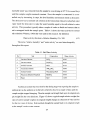
Table 4.1. Salt Water Activity
No
Salt
Composition
Water Activity
1
Calcium Chloride
CaCl2
0.295
2
Calcium Nitrate
Ca(N03)2
0.505
3
Sodium Chloride
NaCl
0.755
4
Ammonium Sulfate
(NH4)2S04
0.800
5
Sodium Tartrate
Na2C4H406,2H20
0.920
6
Potassium Dihydro Phosphate
KH2PO4
0,960
7
Water
H2O
1.000
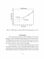
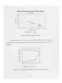
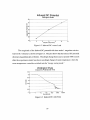
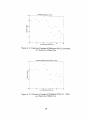
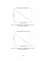
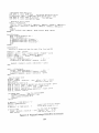
Another procedure that was tried for the drying stage was exposing the sample to
ambient air (as the ambient air in the lab is relatively dry), for a couple of days until the
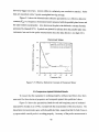
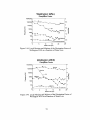
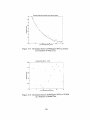
sample weight stopped changing. Then the sample was brought back up to its original sample weight lUce the oven dried one. Figure 4.3 shows a typical sample relative weight (the
ratio of current sample weight to its original weight) changes as a function of water activity
for the two cases of drying. Both methods brought the sample back to its original weight
at the sample's native water content.
29
Wellington Shale Samples
1.01
1.005
Oven-Dried Samples
0.9651:
0.96
0.1
0.2
0.3
0,4
0.5
0,6
0.7
0.8
0.9
Desiccator Activity
Figure 4.3 Weight Change as a Function of Water Activity (Adisoemarta et al., 1995)
4.4 Shale Properties
The two shales used in this research were Pierre and WeUington. The Pierre Shale,
dark grey in color, is from the Upper Cretaceous age and was cored in eastem Colorado,
The WeUington Shale is dark grey in color and from the Cretaceous age, but with a lower
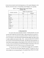
clay content than the Pierre, This shale was cored in central Utah, Table 4,2 shows the results of the X-ray diffraction tests for weight % of both samples.
Using nominal values of density for each component, the grain density of Pierre is
2,73 g/cc and for Wellington is 2.71 g/cc. Water content of the shale samples were determined from thek native and dried weight, and were found as 6.4% and 2.78% by weight for
Pierre and Wellington, respectively. Total porosity of Pierre at its native state, defined here
30
in terms of the moveable water by the drying process, is 14.9%, and for WelUngton is 7.0%.
The CEC of the Pierre shale is 19.8 meq/lOOg, and for WeUington is 9.4 meq/lOOg.
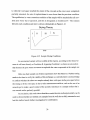
Table 4.2. X-Ray Diffraction Bulk Analysis Results
(Javalagi, 1990)
Weight % in CrystaUine Portion
Crystalline Components
Pierre
Wellington
Smectite
9
0
Illite
20
12
Kaolinite
2
2
Chlorite - Fe
2
1
Calcite
1
14
Dolomite
1
5
Pyrite
4
4
Feldspar - Na
9
5
Feldspar - K
9
2
Quartz
43
56
4 ^ Preservation Fluid
One question that came up during the research is "what fluid should we use to preserve the shale sample that wiU retain the shales' original physical/electrical properties?"
The customary preservation fluid in the petroleum industry is kerosene, but there was no
known investigation on the effectiveness of preserving shale samples other than kerosene
is readily available and inexpensive (Hale, 1992). A good preservation fluid is needed for
this research for both long and short term storage. The long term storage requUement is to
ensure that the sample properties wiU not change with time, and tiie short term requirement
is for the confinement fluid during each of the electromagnetic measurements on the sample
so that the sample will not be in contact with air to avoid drying the sample.
To answer the above question, four different fluid samples and two test methods
were used. The fluids tested were generic kerosene, Isopar M ' ^ ^ (a mineral oil), Silicon
Oil (a synthetic oil), and saturated Isopar M. The saturated Isopar M fluid is the regular
31
Isopar M oil that has been saturated with water by mixing the fluid with deionized water in
a glass jar, agitating vigorously and leaving it to settle for one week. The satm-ated oil is
then siphoned off the top portion of the jar at the moment the fluid is tested. The oil is saturated to reduce the tendency of pore fluid to move out into the confining fluid because water solubility of Isopar M, even though very smaU, is already fulfilled by the saturating
deionized water. Silicon OU as a preservation fluid was suggested by Olhoeft (1994). Because this fluid is very viscous, it wiU not enter the sample and also has a very low water
solubility; hence, there is no movement of pore water from the sample to the confinement
fluid.
The two test methods are: (1) measuring the changes in sample buoyancy and relating those changes to the amount of the pore fluid that leaves the sample, and (2) measuring
the changes in the electromagnetic properties of the confinement fluids before and after
sample immersion.
4.5.1 Buoyancy Method
For the buoyancy method, a simple sample holder that was fabricated suspended the
shale sample directly undemeath the analytical balance's main axis and at the same time
unloaded the balance's measurement pan. This sample holder also retains any debris that
falls off of the sample. Figure 4,4 shows the measurement setup.
For the buoyancy method test, each fluid tested used a preconditioned Pierre shale
sample of around 64 gr. of weight, and the changes in buoyancy were recorded at a predetermined time with a personal computer.
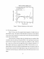
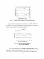
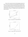
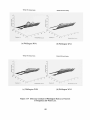
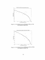
Figure 4.5 shows the comparison of the tested fluids. As can be seen, in the first 4
minutes, all tested fluid showed an increase in weight of the shale sample. This increase of
weight is due to the loss of buoyancy as the shale was shrinking slightly due to water in the
pores that was in contact with the confining fluid tiiat left tiie pore space into the fluid. The
Silicon oU was the worst performer as the rate of loss was the highest. Kerosene, the defacto preservation fluid in the industry, was not much better as the fluid continuously shrank
the sample by taking the pore fluid out. The next fluid, Isopar M, showed an interesting
trend. The first 4 minutes, it made the sample shrink, but then the sample slightiy swelled
32
due to a counter flow of oil into the sample. After 15 minutes the rate of water loss overcame the incoming rate and made the sample shrink again. By saturating the oU, this behavior can be slowed down and takes 3 times longer to occur
Computer
Digital Balance
Sample Hanger
Shale
Fluid Container
Figure 4.4 Buoyancy Measurement Semp (Adisoemarta et al., 1995)
Pierre Shale
1
!•
-
1
r"
~"
1—
T
1
1
14
12-
Silicon Oil
10&
//
i
t
8
/
'.
—I
!
'
J
'
X
/
Kerosene
.-
-
X
/'-•
/
i
/
-
;
/ Isopar M*
*•'
•
!
r
•••
0
/
/
If'.
'
i \
!
0
/
#
i. •
1
/
/
^——"^
Saturated Isopar M
.
1
1
20
40
60
_I
80
1
1
100
120
.J..
140
..
..
'
160
Time, Minutes
Figure 4.5 Buoyancy Changes of Shale (Adisoemarta et al., 1995)
33
180
The conclusion so far is that for the 100 minutes requirement for the sample to be
in fluid before the next electromagnetic measurement, the saturated isopar M is tiie fluid of
choice as the sample shrinkage is the smallest compared to other confinement fluids. For
the long term storage requirement, the best fluid is sUicon oU as the weight stops changing
after 50 minutes. However the cost is prohibitive. Kerosene shows the weight change
tapers off and flattens out eventuaUy. Thus for practical purposes, kerosene is stUl a good
long-term preservation fluid.
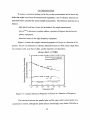
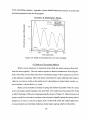
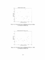
4.5.2 Electromagnetic Method
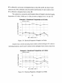
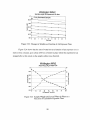
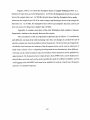
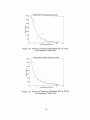
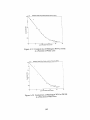
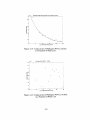
Another method that shows that fluids are exchangedfiromthe sample into the preservation fluid is the analysis of the electromagnetic properties of the preservation fluid itself
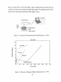
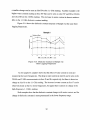
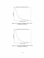
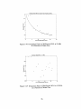
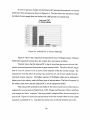
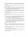
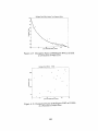
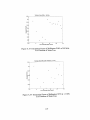
Figure 4.6 shows the change in conductivity of the preservation fluid after a Wellington shale has been immersed for 3 months. This long duration testing was executed to
decide whether saturated Isopar M oil is a good long-term sample preservation fluid. As
can be seen, the conductivity of the original fluid was around zero, and sUghtly increased
at the higher frequency end due to impurities in the deionized water used to saturate the oil.
The fluid that was in contact with the Wellington shale showed a huge increase, at the high
frequency end, in conductivity. This conductivity increase can be attributed to ions that
moved out of the pore space into the preservation fluid. Unfortunately no ion-analysis was
done on this fluid to determine exactly what specific ion moved into the fluid.
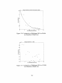
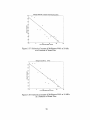
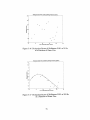
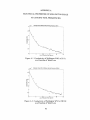
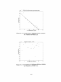
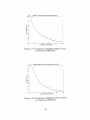
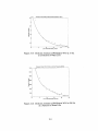
Figure 4,7 shows the change in the dielectric constant of the preservation fluid. The
clean fluid has a dielectric constant of around 2.25 and peaks at 2.44. The fluid that contained the shale sample showed a noticeable increase and peaked at 2.86. As the dielectric
constant contrast between oil and water is 2 to 80, it can be concluded that the amount of
water in the preservation fluid increased; hence, the amount of pore water in the sample decreased, and the sample properties could not be assumed to be the same as before the immersion.
34
Isopar After 3 Months with Wellington
0.008
I
I
I I I I
-I
r
O Clean Fluid
• 3 Months
(S/m
0.006
fJ
0.004
iductiv
2r
0.002
O
o
0.000
j_L
-0.002
2x10^
5x10^
'
10^
2x10«
I
.
I
5x10«
•
I I
10^
2x10®
Frequency (Hz)
Figure 4.6 Conductivity Changes After Shale Immersion
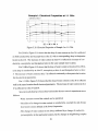
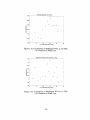
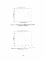
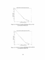
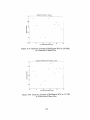
Figure 4.8 shows the dissipation factor changes after the shale sample immersion.
As the fluid is more conductive, more energy is lost as heat. The medium, therefore, is more
electrically lossy and reflected as an increase on its dissipation factor.
Isopar After 3 Months with Wellington
3.0
2.8
«
c
o
O
-
2.6
2.4
-
o
b
2.2
2.0
1.8
2x10^
5x10''
^CP
2x10«
5x10«
10® 2x10'
Frequency (Hz)
Figure 4.7 Dielectric Constant of Confining Fluid
35
Isopar After 3 Months with Wellington
0.2 n—I—r—r
O CIsan Fluid
• 3 Months
B
O
0.1
03
C
.2
^//V n^^^^^^
CO
.955
w
0.0
-0.1
2x10^
1
1
I
I
5x10^
I
1 I 1
10^
2x10^
I
5x10^
I
I t I
10®
2x10®
Frequency (Hz)
Figure 4.8 Dissipation Factor of Confining Fluid
The conclusion of this investigation is that there are fluid exchanges between pore
water and the fluid for all preservation fluids that have been tested. Hence one should question the representativeness of a sample after its storage influidas the pore fluid will not have
the same properties as the original one. The rate of fluid exchange can be reduced by presaturating the preservation fluid with deionized water. To avoid this exchange of pore fluid,
especially for a long term sample storage, the non-fluid contact method should be utilized,
such as sample waxing.
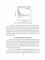
4 6 Air Entrapped In Shale r Adisoemarta. 1995^
One question that came up in this study was whether the shale sample was fully saturated with pore fluid or not before the experiment started. The partial saturation of shale
wiU create a capillary effect that might significantiy affect the experiment that is in progress
(Forsans and Schmidt, 1994). For example, for the case of electrical measurement, this
capUlary effect will pull the preservation fluid into the sample and mask the actual changes
of electrical resistance of the sample.
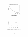
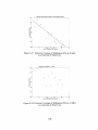
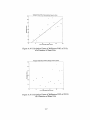
An experiment with Wellington shale was done by exposing tiie sample to air for a
prolonged time to evaporate the pore water while the resistivity and the acoustic travel time
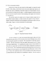
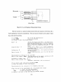
across the sample were recorded. Figure 4.9 shows the measurement setup that uses a pulse
36
generator and a digitizing oscilloscope for the acoustic travel time, and a signal generator
and voltmeter for the resistivity measurement. To ensure that no ionic buUdup (also called
"contact resistance") occurs at the electrode sample interface, the signal generator is set at
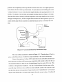
20 kHz. The detail of the electrical and computer hookup is shown in Figure 4.10 which
illustrates that ambient humidity, ambient temperamre, and sample length are also recorded
through a multiplexer box, and the computer that automates the data acquisition process to
ensure that the data wiU be recorded in a relatively fast pace (every 5 seconds) and error
free.
Signal
Generator
Pulser/
Receiver
OsciUoscope
Figure 4.9 Acoustic and Resistivity Measurement Setup
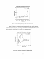
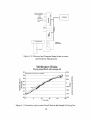
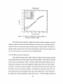
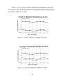
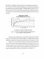
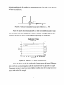
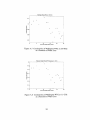
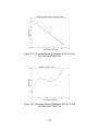
The result of this experiment is shown on Figure 4.11. This plot shows 4 (four) regions with different slopes of either the sample resistivity or tiie acoustic travel time.
Ceramic drying theory by Keey (1991) states that as soon as the fully saturated sample is exposed to aU, there will be pore water evaporation at the sample surface with the rate
of evaporation being less than the rate of replenishment from tiie center of the core. This
condition is designated as Condition I. The rate of replenishment from the center of the
core wiU drop with time as there wUl be less water available, and this wiU create the condition II, where the rate of evaporation is larger tiian the rate of replenishment. As the amount
of pore water diminishes, void space starts to grow from the sample surface. Condition 111
37
Source (for resistivity)
Sense (for resistivity)
LVDT-1
LVDT-2
Thermometer-1
Thermometer-2
Load
3
a<D
Q.
computer
a.
S
^ ss
o
CM
CO
Output
3
m
m
Q.
5
Digitizing
Oscilloscope
Figure 4.10 Electrical and Computer Setup for the Acoustic
and Resistivity Measurement
Wellington Shale
Drying experiment with sample #3
0
10
15
Time (Hr)
Figure 4.11 Resistivity and Acoustic Travel Time as the Sample Is Drying Out.
38
is when the void space reached the center of the core and as the core is now completely
partially saturated, the rate of replenishment is even lower than the previous condition.
The equilibrium in water saturation condition of the sample wiU be reached after all movable pore water has evaporated, and this is designated as Condition IV. The relation
between each condition and time is shown schematicaUy in Figure 4.12.
Drying Theory
I
II
III
TV
R
At
time
Figure 4.12 Sample Drying Conditions
An unsaturated sample wUl not exhibit all the regions, according to the theory because it wUl start directiy at Condition II, bypassing Condition I, as there are air pockets
that obstruct the pore water movement to replenish tiie water evaporated at the sample surface.
Only one shale sample out of three experiments show this behavior. Further testing
needs to be done to verify tiie validity of this technique, as currentiy there is no knowledge
to confirm whether the other two samples akeady have void space in the pore space before
the testing or if the void space is due to other measurement artifacts, such as the use of an
acoustic gel to make a good contact of the acoustic transducer or a sample surface that is
not smooth and/or perfectly parallel.
In conclusion, this result shows tiiat this acoustic/electric method potentially can be
used to check whether new drilled core samples from tiie weU site are fully saturated or not,
but this method needs further investigation for confirmation.
39
CHAPTER V
ELECTROMAGNETIC MEASUREMENTS
This chapter wUl describe the experimental procedures in electromagnetic measurement that are used in this research and wUl include discussion on error sources, measurement equipment, reference materials, scope of research m frequency, and several results
from shale samples.
5.1 Error Sources
Olhoeft (1981) discusses in detail several error sources in typical electromagnetic
measurements either on dry or wet samples. In dry sample measurements, errors occur due
to current leakage around the sample through the sample holder, cable coupling, fringing
effect, and instrument drift. In wet samples, the above error sources can occur along with
errors from current leakage due to wet sample surface, contact impedance between the electrodes and the sample, and chemical reaction between sample and sample holder.
The cable coupling errors (due to capacitive and inductive affect on the cables) are
eliminated by using current driven shielded cable setup where the shield will have a current
of the same magnitude but in the opposite direction than the signal, thus cancelling the inductive effect. This shielded cable also eliminates the capacitive interference between cables. Fringing effect is minimized by using samples as thin as possible. Contact impedance
error, between the electrodes and the sample, is minimized by using a four-terminal setup
where the potential electrode is located outside the charge build-up, and also by using a potential electrode with a high input impedance input so no significant current flows through
the potential electrode to the sample. Chemical reactions between sample and sample holder are minimized by using inert sample holders (plexyglass), and non-reacting preservation
fluid (to keep the moisture in the sample from drying out during the measurements).
The last error soiurce, the instrument noise and drift, are handled by averaging several consecutive measurements and comparing daily readings against several reference materials, respectively.
40
5.2 Scope of Research
Each shale sample in this research wiU be measured for its electromagnetic properties in the range from 5 Hz up to 1,3 GHz (1.3x10 Hz) using two different measurement
setups, as shown in Figure 5.1. Also shown in the figure are the commercially available
logging tools; thus it would be easy to implement the results of this study to the actual weU
log reading. The width of the frequency span of this study, which is about 7.5 orders of
magnitude in frequency (5x10^ to 1.3x10^ Hz) encompasses almost half of the current techniques in electromagnetic measurement, which is 17 orders of magnitude (10' to 10 Hz)
as reported by Olhoeft (1981).
1
Open-Ended
Coaxial Probe
High-Frequency Setup
Parallel Capacitance
Method
Low-Frequency Setup
I
1 I I mill
o
>o
o
o
oo
"g
O
^^
"^^
§•§
I
I MiMiJ I
J
I mniil
i i mini
i iiiiml
ml i i iiiiiil
s^
i
I i iiiiiiil
10° 10^ 10^ 10^ 10"^ 10^ 10^ 10^ 10® 10^ 10^°
Frequency (Hz)
Figure 5.1 Frequency Span of the Measurement Equipment and
Current Conunercial Logging Tool Frequencies
S ^ Measurement AnnaraUis
The complex electrical parameters of the sample were measured over two frequency
ranges using two different measurement techniques.
41
5.3.1 Low Frequency
The low frequency range, from 5 Hz to 12 MHz (1.2 x lO'^ Hz), is measured using
an HP 4192A impedance analyzer m conjunction with a paraUel-plate measurement technique as shown schematically in Figure 5.2.
Electrodes
Sample
Silver metal membranes
Figure 5.2 ParaUel-plate Measurement Technique
This setup is the 4-port parallel-plate technique in which the current and voUage
measurement electrodes are separated by a thin porous conductive plate. The electrodes are
gold-paUadium coated brass porous plates, and the separator plates are PoreTTVyf
tics
sUver metal membranes, a product of Osmonics.
In the beginning of the research, the 2-port parallel-plate method was used instead,
using the HP 16451A Dielectric Test Fixture, but due to induced DC current that was generated by the shale sample during measurement, the 4-port was then implemented through
custom built cabling that also preserves the cable shielding feature of the 2-port fixture.
The analyzer is controlled via an IEEE-488 (GPIB/HPIB) bus from a microcomputer. Software has been written to acquire the measurements. This allows the researchers to
acquire data with fine frequency resolution and reduce operator error, as the equipment
readings will be saved directly to the storage media, for further processing. A fixture has
been built for shale measurements submerged in preservation fluid. This fixture will improve the data because the sample wUI keep its moisture since there is no air contacting the
sample to dry it out.
42
5.3.2 High Frequency
The high frequency range starts at 20 MHz (2 x 10^ Hz) and ends at 1.3 GHz (1.3
X 10 Hz). Measurements are made using an HP 8752A network analyzer. This instrument
actually consists of two parts: the network analyzer and the display processor. An
open-ended coaxial probe, HP 85070B, is used to determine the reflectivity, S*n. of the
sample. This is converted to real and imaginary permittivity using the manufacturer's software, which incorporates an algorithm for correcting for geometric effects in the probe.
Figure 5.3 shows schematicaUy the open-ended measurement technique.
Probe
&=3
Sample
Figure 5.3 Open-ended Measurement
The instrument is calibrated by measuring three well-known dielectric mediums,
also called calibration standards. The default calibration standards for this probe are air, a
short circuit, and deionized water. This calibration standard is also called "Air/ShortAVater" method. Other calibration standards for the instrument are "Load/Air/Short," where a
50 ohm coaxial load is substituted for water, and "User Defined," where three known standards can be described and and their electrical properties measured (HP, 1993). The "Air/ShortAVater" calibration process is always done after the instrument has been on for at least
30 minutes, thus ensuring it has reached its operating temperature, and after around 60 measurements. There is a bug in the Windows^^ version 3.1 operating system that slowly leaks
memory. After around 60 measurements the computer loses all the memory space and this
condition makes the computer run very sluggish; hence a reboot is necessary, and by rebooting, the instrument loses its calibration setup.
All shale dielectric measurements were done by taking 5 consecutive readings, and
the averaged value is the one reported herein.
43
5.4 Calibration Check
To ensure a consistent reading on the day-to-day measurements and to detect any
drifts that might occur from the measurement equipment, a set of reference materials are
measured before and after the actual sample measurement. The reference materials are as
foUows:
- light plastic and heavy brass for the balance, for weight measurement
- Alcryn ^ (a thermoset synthetic rubber, a product of Dupont) for the low-frequency equipment,
- deionized water for the high-frequency equipment.
Figure 5.4 shows the complex electrical properties of Alcryn as a function of frequency. Alcryn was selected as a reference material because at 1 MHz, it has a high dielectric constant value, near that of shale, and the material is not hazardous.
Alcryn ALC-1170BK
15
I
I I lllll|
1 I I lllll|
1 1 llllll[
1 I llllll|
1 I llllll{
1 I Mill!
Sample thickness: 2 mm for parallel plate
25 mm for coaxial probe
Parallel plate ciiameter: 5 mm
o
13
>%
•4-^
CD
>
CD
3=
III
CO
C/J
CD
CD
Q_
0)
>
'~
(.i
0)
it=.
UJ
r
o
t5
C/3
10
rrnil
c
o
>
ion
O
CO
^ett^eo'^
^rT^-s^-
. ^
\
c
CD
E
Q
Open-ended
Parallel-plate
r I I mill
104
105
I I I iiml
106
i i i null
10^
I
IQS
i i i mill
10^
I
ii'i'i'
10^0
Frequency (Hz)
Figure 5.4 Complex Electrical Properties of Alcryn as a Function of Frequency,
The transition between the paraUel plate and tiie open-ended coaxial probe measurements is smooth, altiiough the probe data are increasingly noisy below 200 MHz as
44
shown by bigger error bars, Alcryn rubber is a relatively non-conductive material. Probe
data are smoothed with a 5-point unweighted moving average.
Figure 5,5 shows the dimensionless effective permittivity (i.e. effective dielectric
constant, 8^^) vs. frequency of deionized water measured with the parallel-plate fixuire and
the open-ended coaxial probe. Also shown on tiie plot is the dielectric constant fonnula
presented by Hasted(1973). Symbols are plotted for all datafi:omthe paraUel-plate measurements, but not for the probe measurements since the data density is too high (201).
Deionized Water
10^
I I llllll|
o
1 I llllll|
1 I llllll|
1 I I IIIH
Symbols are plotted for all data from
parallel-plate, but not for probe since
data density is too high (201 points).
w
II
%
1 I llllll{
10"*
-
c
B
c
o
o
o
CD
>
10^
^
10^
Probe
UJ
Hasted data
I I I null
10^
10'*
10^
I I iiiiiil
10^
I I I mill
ml
I
10''
10^
10^
10^°
Frequency (Hz)
Figure 5.5 Effective Dielectric Constant of Deionized Water
5.5 Comparison Against Published Results
To ensure that the equipment is working properly, methanol and brines have been
measured for their electrical properties and compared against their published values.
Figure 5.6 shows the permittivity (both the real and imaginary part) of methanol
measured by Jordan et al. (1978), overlaid with the measurement of this dissertation. The
dissertation measurements agree with the published data, suggesting that the high-frequency open-ended coaxial probe is working properly. Accuracy of the probe measurement is
45
demonstrated over the frequency range of 20 MHz to 1.3 GHz, although tiie manufacturers
design Umit is > 200 MHz.
Figure 5.7 shows the effective conductivity of NaCl and KCl brines at 2000 ppm
concentration, at ambient (60°F) temperaUire, measured with the open-ended coaxial
probe. Also shown on the plot is the conductivity of NaCl and KCl taken from Charts
Gen-8 and Gen-9 of the Log Interpretation Charts (Schlumberger, 1995).
Methanol
o
15
40
3
m
CD
O
< •
^
10
CD
35
Q.
o
•D
(D
C
o
o
o_
30 o'
o
o
CD
>
o
Cfl
CD
*•—
«+—
3
CD
CO
(Ti
^_g)
c
g
w
c
0
25 §=
CO
Jordan
Marsland
Adisoemarta
CD
E
I
10^
I 11 n i l
J
10^
\
V
I
I I, I
o
I I I MI
10^
20
10^°
Frequency (Hz)
Figure 5.6 Complex Electrical Properties of Methanol
5.6 Varying the Sample Water Content
The main objective of this dissertation is to measure the shale sample's complex dielectric properties as a function of water content; hence, the water content has to be modified in a controlled scheme for each sample. There are several ways that have been used
for this research to change the amount of water in the sample, namely the desiccator, electrophoresis, and air drying method.
46
NaCl and KCl (2000 ppm)
1.0
I I I I ITTT]"
-
0.8
T i l l III
I I KIT
I I iiiiii|—I
I iiiii!|—I
I I I rill
DC Conductivity from
Schlumberger chart book
NaCl - 0.37 S/m
KCl - 0.35 S/m
E
CO
0.6
NaCl from
Schlumberger
chart book
"o
rj
•D
C
0.4
NaCl
5^
o
o
CD
>
•C
KCl
0-2
NaCl
0.0
I I I mill—I I I mill—I I " " I I I
KCl from
Schlumbergerchart book
CD
UJ
^o'
10-
10^
10^
' I """I
10^
il
10^
I
I
10 10
Frequency (Hz)
Figure 5.7 Effective Conductivity of NaCl and KCl
5.6.1 The Desiccator Method
Figure 5.8 shows a plot of the complex electrical properties of a shale for the complete frequency range. The sample is a Pierre shale that was measured at 4 (four) different
water contents after being kept for several days inside various desiccators that had the particular water activities indicated.
The fact that the two frequency ranges were measured using two completely different methods makes the spUcing of the spectra difficult. After improving the measurement
fixture for the low frequency setup, the two ranges were combined in a single, continuous
plot. A gap exists on the plot since the upper Umit of the low-frequency equipment is 13
MHz while the high-frequency equipment starts at 20 MHz. The fact that the two completely different measurement methods, the parallel-plate for the low frequency range and
the open-ended coaxial probe for the high-frequency range, show approximately the same
conductivity trend with frequency confirms the accuracy of the both measurements to some
degree.
47
Pierre #2
10^
I
' ' """I
r-PTTTTTTI
r i lllllll
1I
I
1 I ||||||[
I
I
I
10^
IQS
10^
r
• g-0.505-IA
" g-0.800-IA
• g-0.92-IA
o g-0.75S-IA
• g-0.505-NA
'^ g-0.800-NA
• g-0.92-NA
3 g-0.755-NA
NA = Network Analyzer
lA = Impedance Analyzer
10^
10"
10C/D
10-^
lO"*
10-5
I I Mlllll
10"®
10"
10^
1 I I mill
10«
1010
Frequency (Hz)
Figure 5.8 Effective Conductivity of Pierre Shale as a
Function of Water Content
The author has been unable to explain the fact that on the low-frequency range the
effective conductivity increases with increasing water content, but on the high-frequency
range, the effective conductivity drops with the increase of water content. The author acquired another instrument that will work on that frequency gap to get more insight on this
fact, but, unfortunately, the instrument arrived malfunctioning.
5.6.2 The Electro-osmosis Experiment
One method to change water content of shale is to impress a direct electrical voltage
on the sample that wUl move the water to one side of the sample. This method is called the
electro-osmosis method (Rose, 1980). The theory behind this method is that the cations
(positively charged ions) and anions (negatively charged ions) wUl move to the charged
electrodes to satisfy the system's neutrality. So cations wUl move towards the anode and
the anions will move towards the cathode. As the anions are in the pore water, the movement of the anions will also bring the pore water to the cathode side. On the other hand,
the cations are on the clay platelets, so they wUl not move. After the sample is impressed
48
with the voltage for a period of time, the sample is cut laterally to preserve the water content
of each particular location. The individual sUces are then analyzed for water content,
Brinell hardness index, and the complex electrical parameters at various frequencies. This
method is described schematically in Figure 5.9.
o^
Shale sample
Cathode
i
Anode
After sUcing
(D(D(D(D(D(D(D
Figure 5.9 Electro-osmosis Method
The samples for tiiis experiment are two Pierre shales, designated as Sample H and
Sample I. These shale samples were received from SheU BeUaUe Research Center in Houston, where researchers from SheU conducted the electro-osmosis process and the Brinell
hardness (BHN) measurement.
Figure 5.10 shows the electrical current across each sample as a function of time. It
can be seen that the current decreases with time as tiie ion buUdup at tiie electrode reduces
the conductivity of the system.
Water content and BrineU hardness number for each slice of Sample H is shown in
Figure 5.11 and Figure 5.12 shows the measurements for Sample I. As can be seen, both
samples show that water is more concentrated at the cathode end and decreases towards the
anode end, as expected from the electro-osmosis method, and as the sample gets drier, it
gets stronger and harder, as indicated by tiie increasing BHN towards the anode end.
49
Electro-osmosis Current: Pierre Shale
Shell Samples
,8)
16 -
:
:
:
14 •
^ <^ 12 -
;
c
2
8 -
i
O
6 -
i
4 -
\
2 -
i
1
0 1
i
;:
•
i
:i:::::*:-x:.::::::i:::::::
•
1
1
1
•
1
1 1 1 i 11
1
:
1 i
1
1 1 1 11
10
1
v^j^
1 , 1 1 , ^ , 1
100
.
1000
i
1
.
i <,
10000
Elapsed Time (min)
LfJ Sample H E Sample 1
Figure 5.10 Electro-osmosis Cmrent
Even though Figure 5.11 shows the water content and BHN of sUce HIO, because
the sample broke off during sample handling, there are no data presented for the electrical
properties.
9
X
m
-I
h
'
„
8 -
*
•
-^1
•
A
'•
"•>-».»,^
i y\
1
Wat er Cont
CD
1
b
tt-^—'
•
H2
H3
H4
H5
H6
S
Water% S
H7
H8
H9
HIO
BHN
Figure 5.11 Water Content and BHN versus Distance for Sample H
50
^
A .-. . ^
'
'
'
^ * * * * ^ * ' ^ j .
14
15
-
'
^
1
1
^
1
01
05
-si
(D
i
(1
i
'
J
Water Content (%wt) or BHN
r
11
12
13
16
17
18
H»-l W a t e r % t>«d B H N
Figure 5.12 Water Content and BHN versus Distance for Sample I
Figure 5.13 shows the dielectric constant of Sample H at 20 kHz, 2 MHz and 1.1
GHz (those are the Dual Induction, MWD tool, and EPT tool frequencies, respectively) as
a function of lateral distance from the cathode to the anode.
Sample H
Cathode at Slice 1
10000 -1
^
c
1000
«
c
o
O
100
o
(D
b
H2
H3
H
H4
20 kHz H
H5
2MHz ®
H6
H7
H8
H9
1.1 GHz
Figure 5.13 Dielectric Constant of Sample H at
Three Logging Frequencies
As can be seen from Figure 5.13, the change of dielectric constant is more pronounced at low-frequency than high-frequency. For example, the increase in water content
at slice H3 can be seen clearly at sUce H4 at 20 kHz, and slice H5 at 2 MHz reading;
51
a smaller change can be seen at slice H4 at the 1.1 GHz reading. Another example is the
higher water content reading at sUce H7 that can be seen on slice H7 and H8 at 20 kHz
and sUce H8 on the 2 MHz reading. This increase in water content is almost undetectable on the 1.1 GHz dielectric constant reading.
Figure 5.14 shows the dielectric constant response of Sample I at the same three
logging frequencies.
Sample I
Cathode at Slice 1
1000 -t
12
13
H
20 kHz H
14
15
2MHz S
16
17
I
1.1 GHz
Figure 5.14 Dielectric Constant of Sample I at
Three Logging Frequencies
As for sample H, sample I shows that the effect of water content is more pronounced at the lower frequencies. The drop in water content at slice 16 can be seen on the
20 kHz and 2 MHz measurements at slices 15 and 16, respectively, but there is almost no
change at slice 16 on the 1.1 GHz reading. The increase in water content at slice 17 can be
observed clearly at the two lower frequencies, but again there is almost no change in the
high-frequency, 1.1 GHz, reading.
Both samples show that the dielectric constant changes with water content, and the
change in dielectric constant is more pronounced in the lower frequency range.
52
Figures 5.15, 5.16 and 5.17 show the complex electrical properties conductivity
(G), susceptivity (B), and dissipation factor (D) for sample H at the three logging frequencies (20 kHz, 2 MHz, and 1.1 GHz).
Sample H: Electrical Properties at 20 kHz
Cathode at Slice 1
10 -,
^
•m-
CO
0.1 —
b
o
CO
0.01
0.001 - -
o
0.0001
H8
H9
Figure 5.15 Electrical Properties of Sample H at 20 kHz
Sample H: Electrical Properties at 2 MHz
Cathode at Slice 1
10
o
t3
CO
Ll-
c
.o
«
o.
1 --
'vi
v>
Q
o
^
CQ
0.1
0.01
O
o
0.001
Figure 5.16 Electrical Properties of Sample H at 2 MHz
53
Sample H: Electrical Properties at 1.1 GHz
Cathode at Slice 1
'
0.7
*
^
'
I
I
I
.... 1
•
0.6
1
• '•
.'
0.8
'
•
0.9
----1-1
1
0.5
-
0.4
^
0.3
—
"
'
1
T
^
^
,
1
#•' •
•
0.2
0.1
1
,
1
'
'
:
0
H2
H3
H4
^
GS
H5
BS
H6
H7
MB
H9
D
Figure 5.17 Electrical Properties of Sample H at 1.1 GHz
For 20 kHz, Figure 5.15 shows that conductivity (G) and susceptivity (B) increase
as water content increases. For example, the increase of water content at slice H3 can be
seen on the conductivity and susceptivity at slice H4. When water content drops at slice
H5, the effect on electrical properties can be seen at the same location, and when water content rises again at slice H7, the increase is reflected in the electrical properties at the same
location. The dissipation factor also changes as the water content changes. The general
trend is that conductivity and susceptivity are decreasing from the cathode end to the anode,
as is water content.
For 2 MHz, Figure 5.16 shows that the drop of water content at slice H5 is detected
at slice H6 on both the conductivity and susceptivity. The water content increase at slice
H7 can be seen on conductivity right at that slice and on susceptivity on sUce H8. The dissipation factor is also reflecting the changing water content, as shown in slice H7 where water content is slightiy increased, which is reflected in the slightiy increasing dissipation
factor.
For 1.1 GHz, Figure 5.17 shows that the increase of water content at H3 can be seen
at slice H4, the drop of water content at H5 can be seen at H7, and the increase at H8 can
be seen at H9. There is no clear trend of conductivity and susceptivity decreasing from the
cathode to anode. The dissipation factor shows that the increase of water content at slice
54
H3 is reflected by an increase in dissipation factor at sUce H3 and H4, the drop of water
content m slice H5 is reflected at sUce H, and tiie small increase of water content at slice
H7 is reflected in dissipation factor at sUce H8.
The conductivity, susceptivity and dissipation factor of Sample I at the three logging
frequencies of 20 kHz, 2 MHz and 1.1 GHz are shown on Figures 5.18, 5.19, and 5.20.
Sample I: Electrical Properties at 20 kHz
Cathode at Slice 1
10 -t
0.0001
13
12
S
14
GS
15
B^
18
D
Figure 5.18 Electrical Properties of Sample I at 20 kHz
Sample I has a smooth decreasing water content, as shown in Figure 4.25, with two
interesting locations, sUce 16 and 17, that have lower and higher water content, respectively.
Sample I: Electrical Properties at 2 MHz
Cathode at Slice 1
o
ts
to
U-
c
.o
•Jo
o.
w
b
o
;§•
0.01 —
CD
o
O
0.001 —
0.0001
12
13
S
14
GS
BS
15
D
Figure 5.19 Electrical Properties of Sample I at 2 MHz
55
Sample I: Electrical Properties at 1.1 GHz
Cathode at Slice 1
1 -T
0.9 - •
0.8 - 0.7
0.6 4
0.5
•••-
0.2
0.1
-12
S
GS
16
15
14
13
BS
17
18
D
Figure 5.20 Electrical Properties of Sample I at 1.1 GHz
For 20 kHz, Figure 5.18 shows that the drop of water content at slice 16 is reflected
on both conductivity and susceptivity at slice 15, with a corresponding drop in dissipation
factor in sUce 16. The mcrease of water content at sUce 17 is reflected in increase of conductivity, susceptivity and dissipation factor m the same sample sUce location.
For 2 MHz, Figure 5.19 shows that the drop of water content at location 16 is reflected in drop in conductivity at sUce 15, susceptivity at sUce 6, and dissipation factor at slice
5. The increase of water content at slice 7 is reflected consistentiy at tiiat particular location
for the electrical parameters.
For 1.1 GHz, Figure 5.20 shows that the drop of water content at slice 16 is reflected
weU in the same location for all electrical parameters. The mcrease of water content at slice
17 is reflected on sUce 17 and 18.
Several results that have been observed from the electro-osmosis experiment are as
follows:
- Water increases toward the cathode end as predicted
- The affect of a change in water content on conductivity, susceptivity and dissipation factor is more defined at the lower frequencies,
- The change of water content is not always reflected by a change of conductivity/susceptivity at that particular location, but by changes at neighboring samples.
56
5.6.3 The Air Evaporation Method
Another way to reduce the water content in a shale sample is to expose the sample
to air for a whUe, letting a small amount of pore water at the sample edge evaporate, and
then allow the water to redistribute evenly before another set of electromagnetic measurement is performed on that particular sample. A carefuUy arranged air exposure procedure
has to be executed so that the amount of water remaining in the sample can be monitored
in a controlled way.
The procedure exposes the sample to air for 5 minutes while the sample sits in an
opened digital analytical balance, and then resaturates the sample for 2 hours while the
sample is immersed in fluid before the electromagnetic measurement is taken on that particular sample. Figure 5.21 shows the timeline of one shale sample.
Time
•
•a
'a
'3
a
I
1
•§
•§
FuUy saturated sample I "^ I 2 hrs. in Isopar
equilibration
dessicator
@0.96
I '^ I 2 hrs in Isopar
I
equilibration
I '" I 2 hrs in Isooar
j
equilibration
I
\
I -^ | 2 hrs. in Isopar
\
equilibration
EM Measurements
Figure 5.21 Experiment Procedure TimeUne
As shown in Figure 5.21, a fuUy water saturated shale sample is taken out of a desiccator that has water activity of 0.96, the water activity of native Wellington shale, and then
its electromagnetic properties are measured. This measurement is for tiie fully saturated
condition. After tiiis measurement is done, the sample is tiien exposed to air for 5 minutes
in an opened digital balance. To re-equilibrate tiie sample to the new water saturation condition after the sample edges are exposed to ak, the sample is inunersed in inert fluid, Isopar, for two hours. This re-equilibration time has been determined from one test that shows
the changes of electrical properties stop changing after around 90 minutes, as shown in Figure 5.22 Hence if the equUibration time is set for 120 minutes (2 hours), then it can be safely assumed that the water saturation has re-equilibrated completely. After the sample has
57
assumed the new equilibrium condition, another set of electromagnetic measurement is
done. The sequence repeats again untU the sample shows a visible crack on the sample surface that indicates aU has entered the sample. As akeady mentioned in the error sources
section, due to the low value of the dielectric constant and the non-conductive nature of air,
even a thin gap of air will skew the measurement resiUt, and hence the data wUl not be representative.
Wellington WN2
During Equilibration after 1st 5min Air
0
10
20
20 MHz
30
40
50
60
Time in Fluid (min)
70
80
90
100 MHz - ^ < - 250 MHz - & - 1.1 GHz
Figure 5.22 Relative Change of Conductivity at Various Frequencies as a Function of Time in Inert Fluid
The actual sample weight changes as a function of air exposure time in the digital
balance for every measurement set are shown in Figure 5.23. The figure shows that sample
weight has a constant rate of weight drop, which means the rate of evaporation is constant.
Figure 5.24 is a replot of the previous plot, but in tiiis plot the end weight of the 5
minutes of air exposure is plotted against the cumulative air exposure time. From oven drying of the sample, the amount of moveable water is 2.4 grams. By dividing the actual water
loss (the decrease in sample weight) to tiie total moveable water, the actual water loss in
percent is calculated, which then plots on the secondary Y axis in Figure 5.24.
58
Wellington WN-2
Sample weight vs Exposure to Air time
67-
Fully Saturated Sample
Figure 5.23 Changes in Weight as a Function of Air Exposure Time
Figure 5.24 shows that the rate of water loss as a function of air exposure time is
more or less constant, up to about 22% loss of water in place where the experiment was
stopped after a thin crack on the sample surface was observed.
Wellington WN2
Assuming 2.4g of water 01P
10
20
30
40
50
Air Exposure Time (min)
60
Figure 5.24 Sample Weight and Loss of Water in Place as a
Function of Cumulative Exposure Time
59
Figure 5.25 shows a typical error bar plot of the electromagnetic measurement of a
shale. As error-bar can not be plot in the customary log-log plot for conductivity. Figure
5.26 shows the variance plot which shows the span of the variance (the data plus and minus
the error-bar) with the actual data removed. The plot shows that the error bar is very small
along the frequency of interest. The largest error bar, at the lower end of the high frequency
measurement range, is less than 7%. This largest error bar is at around 20 MHz where the
data are a bit noisier.
WNl - Error Bar Plot
0.18
x10°
Figure 5.25 Error Bar Plot of a Shale Measurement
WNl - Error Bar Plot
10 E
X
10'
/
h°'
2-
>
TS
-:
lio-'
O
10"
'•
10*'10°
^
10'
10^
10*
Frequency (Hz)
io"
1C
Figure 5.26 Variance Range of a Shale Measurement
60
The following figures show the resuk of electromagnetic measiurements on 4 (four)
WelUngton shale samples. The electromagnetic parameters (conductivity, dielectric constant, and dissipation factor) are plotted on the z-axis, as a function of frequency and the
amount of water loss in percent.
Figure 5.27 shows the conductivity of four WeUington shale samples WNl, WN2,
WN4, and WN5 as a function of frequency and water loss. Sample WN3 was not included
in the research as that sample cracked during preparation time. AU plots show a trend of
declining conductivity as frequency decreases and also as the amount of water loss increases. Figures 5.27a and 5.27c show that the two measurement methods more or less create a
continuous trend. Figures 5.27b and 5.27d, however, show a distinct gap in the frequency.
One explanation for the gap is due to heterogeneity of the sample; as different measurement
techniques read different areas, slight changes in properties wUl be recogiuzed more on one
method than the other. The low frequency setup that uses the parallel-plate method will
read the whole sample surface and across the sample thickness, basically averaging the
property of the medium. The high frequency setup uses an open-ended probe that has a diameter of less than half of the sample diameter; thus this probe only reads whatever is right
on the center of the sample surface. Hence a high spot on the center of the sample will easily skew the high frequency measurements.
To better look at the changes of conductivky as water content decreases at logging
tool frequencies, one can do a cross-section cut on Figure 5.27 parallel to the water loss axis
at the specific tool frequency. Figures 5.28 through 5.33 shows conductivity of sample
WelUngton WNl at 35 Hz (Deep Laterolog tool), 280 Hz (Shallow Laterolog tool), 20 kHz
(induction type tool), 10 MHz, 250 MHz (MWD tool), and 1.1 GHz (dielectric tool). Ignoring the first data point tiiat has a lower conductivity than tiie others, the conductivity
drops rapidly in the first 5% water loss and then levels off, as seen at 35 Hz, 280 Hz, and
20 kHz in Figure 5.28, 5.29, and 5.30, respectively. This drop in conductivity is less defined
at 10 Mhz and vanishes at 250 MHz and 1.1 GHz.
Figure 5.34 shows the dielectric constant as a function of frequency and water loss
in percent, and Figures 5.35 up to 5.40 show the dielectric constant at various logging tool
frequencies as a function of water loss.
61
Wellington WNl Absolute Heading
10°
Wellington WN2 Absolute Reading
0
(a) WelUngton WNl
(b) WelUngton WN2
Wellington WN4 Absolute Reading
Wellington WN5 Absolute Reading
(c) Wellington WN4
(d) WelUngton WN5
Figure 5.27 Conductivity of Wellington Shales as a Function
of Frequency and Water Loss.
62
y^ ^Q-s
Wellington Shale WNl at Deep Laterolog Frequency (35Hz)
10
15
Loss of Moveable Water, percent
20
25
Figure 5.28 Conductivity of WelUngton WNl at 35 Hz
as a Function of Water Loss
, ^Q-s
Wellington Shale WNl at Shallow Laterolog Frequency (280Hz)
10
15
Loss of Moveable Water, percent
20
25
Figure 5.29 Conductivity of WeUington WNl at 280 Hz
as a Function of Water Loss
63
X ^Q-»
2.5|—i
Wellington Shale WNl at Induction Tools Frequency (20kHz)
1
1
1
1
-ii.5
CO
o
O
0.5
*
5K
10
15
Loss of Moveable Water, percent
*
20
25
Figure 5.30 Conductivity of Wellington WNl at 20 kHz
as a Function of Water Loss
xio
Wellington Shale WNl at
10 MHz
10
15
Loss of Moveable Water, percent
20
25
Figure 5.31 Conductivity of WeUington WNl at 10 MHz
as a Function of Water Loss
64
Wellington Shale WNl at 250 MHz
0.06
10
15
Loss of Moveable Water, percent
20
25
Figure 5.32 Conductivity of WeUington WNl at 250 MHz
as a Function of Water Loss
Wellington Shaie WNl at EPT Frequency (1.1 GHz)
0.22
JK
0.2
X
0.18
«
^
-
(S/I
-?0.16
i
*
:>o.i4
o
•n
•o
c
^0.12
*
*
0.1
-
J«
*
*
*
*
X
^
*
0.08
10
15
Loss of Moveable Water, percent
20
25
Figure 5.33 Conductivity of WeUington WNl at 1.1 GHz
as a Function of Water Loss
65
Figure 5.34 shows that the dielectric constant of WeUington shales is not "constant"
along the frequency axis, decreasing in magnitude as the frequency increases. Also the
jump of the dielectric constant at the measurement gap can be seen on the plots. Currentiy
there is no explanation for this occurrence of the gap. At logging tool frequencies of 35 Hz
and 280 Hz, shown in Figures 5.35 and 5.36, the dielectric constant of WelUngton WNl
shale drops rapidly in the first 10% of water loss as the sample dries out. This trend changes
into a more-or-less linear fashion at 20 kHz and 10 MHz, as shown in Figures 5.37 and 5.38,
respectively. At higher frequencies, 250 MHz and l.I GHz, no pattern was observed, as
shown in Figures 5.39 and 5.40, respectively.
Figure 5.41 shows the dissipation factor of WelUngton shales as a function of frequency and water loss. Similar to the dielectric constant plots, there is a gap in the dissipation factor at the frequency gap that the author is unable to explain. Also the distinct peak
(local maxima) is clearly seen on the plots, and the magnitude of the peak decreases as the
sample gets drier. Also a local minima can be seen on the figure, but the details are obstructed behind the "mountain." Figures 5.42 up to 5.45 plot the characteristics of the local
maxima and minima of Wellington shales as a function of water loss, so the maxima and
minima can be better analyzed. Those figures show that both local maxima and local minima drop both in frequency and magnitude as the sample gets drier. This characteristic is
consistent on all of the four samples. The outcome is very interesting because either by using those characteristics individually or in combination, sample's water content can be determined. One example of appUcation is on well logging. By comparing the dissipation
factor characteristic from different logs on the same formation type, the formation water
saturation can be qualitatively approximated. Another potential appUcation is on time
lapsed MWD situation where the dissipation factor characteristics can be displayed at the
drill floor real time and can be used to predict the onset of wellbore instability. There are
several technical obstacles for applying these methods: the tool must operate at a much lower frequency than that of the current MWD tools, and also be of variable frequency instead
of the single frequency mode of the current tools.
66
Figures 5.46 to 5.51 show the dissipation factor of sample WeUington WNl as a
function of water loss at several frequencies. At 35 Hz, the dissipation factor shows no pattern as the sample dries out. At 280 Hz the plot shows that the dissipation factor peaks
whenever the sample loses 6% of its water content, and then drops down as the sample further dries out. At 20 kHz, the dissipation factor shows an asymptotic decrease, and no pattern was shown for frequencies higher than 10 MHz.
Appendix A contains more plots of the other Wellington shale samples at logging
frequencies, similar to that already shown in this section.
The conclusions of the air evaporation experiment are as follows: (1) conductivity
and dielectric constant drop with increasing water loss; (2) changes in conductivity and dielectric constant are more detectable at lower frequencies; (3) the location and magnitude
of both the local maxima and minima of the dissipation factor can be used as indicators of
shale water content; (4) by comparing the dissipation factor characteristic from different
weU-logs on the same formation type, the formation water satiuation can be qualitatively
approximated; (5) dissipation factor characteristics from MWD tools can be displayed at
the drill floor real time and can be used to predict the onset of weUbore instability; and (6)
weU logging tools and MWD tools need to be modified to work at a much lower frequency
and to be of variable frequency.
67
Wellington WNl Absolute Reading
10°
0
Wellington WN2 Absolute Reading
Frequency, Hz
Moveable Water Loss, pet
(a) Wellington WNl
10°
0
0
Moveable Water Lo&s, pet
(b) WeUington WN2
Wellington WN4 Absolute Reading
Frequency. Hz
10"
Wellington WN5 Absolute Reading
Frequency, Hz
Moveable Water Loss, pet
(c) WeUington WN4
Moveable Water Loss, pet
(d) WeUington WN5
Figure 5.34 Dielectric Constant of WeUington Shale as a Function
of Frequency and Water Loss.
68
Wellington Shale WNl at Deep Laterolog Frequency (35Hz)
14000
12000
10
15
Loss of Moveable Water, percent
20
25
Figure 5.35 Dielectric Constant of Wellington WNl at 35 Hz
as a Function of Water Loss
Wellington Shale WNl at Shallow Laterolog Frequency (280Hz)
3500
10
15
Loss of Moveable Water, percent
20
25
Figure 5.36 Dielectric Constant of Wellington WNl at 280 Hz
as a Function of Water Loss
69
Wellington Shale WNl at Induction Tools Frequency (20kHz)
5
10
15
Loss of Moveable Water, percent
20
25
Figure 5.37 Dielectric Constant of Wellington WNl at 20 kHz
as a Function of Water Loss
Welllngtor Shale WN1 at
7
^
6,8 -
^
10 MHz
1
'
'
'
^
-
)<
6.6
SK
-
•
K)
^
-
O)
Dielectric Constant
6.4
-
5.8
"
5,6
-
5.4
-
•
*
^v. *
\JK
*
M
^
•
* )^\
1
1
10
15
Loss of Moveable Water, percent
20
25
Figure 5.38 Dielectric Constant of WeUmgton WNl at 10 MHz
as a Function of Water Loss
70
Wellington Shale WNl at 250 MHz
10
15
Loss of Moveable Water, percent
20
25
Figure 5.39 Dielectric Constant of WeUmgton WNl at 250 MHz
as a Function of Water Loss
Wellington Shale WN1 at EPT Frequency (1.1 GHz)
10
15
Loss of Moveable Water, percent
20
25
Figure 5.40 Dielectric Constant of WeUmgton WNl at 1.1 GHz
as a Function of Water Loss
71
Wellington WN1 Absolute Reading
Wellington WN2 Absolute Reading
10" 0
(a) Wellington WNl
(b) WeUington WN2
Wellington WN4 Absolute Reading
Wellington WNS Absolute Reading
(d) Wellington WN5
(c) Wellington WN4
Figure 5.41 Dissipation Factor of WeUington as a Function
of Frequency and Water Loss.
72
Wellington WN1
Dissipation Factor
1000000;
-^—m
^
X X
^\/VMinima
3.5
3
2.5^
<a
Maxima
2
i:
C
Q.
1.5 ®
Maxima
1
^"^"s-s-.Q.QE] Mjnima 0.5
10
10
15
Water Loss (pet)
25
20
Figure 5.42 Local Maxima and Mmima of the Dissipation Factor of
WelUngton WNl as a Function of Water Loss
Wellington WN2
Dissipation Factor
3.5
10000000?
1
100^
£3
B-
XA-,-^
Minima
100
0.5
-e—s
10
15
Water Loss (pot)
•
20
^-0
25
Figure 5 43 Local Maxima and Minima of the Dissipation Factor of
WelUngton WN2 as a Function of Water Loss
73
Wellington WN4
Dissipation Factor
lOOOOOOOg
3.5
lOOOOOOi^Minima
3
lOOOOOr
N
O
2.5^
loooq
c
o
Maxima 2
1000=
gl-
Q.
-SS—
lOOi
ic
\
1.5 "^
^
/ «( j»j» Maxima
1C^13—a-
1
^BS3 Minima
1
10
15
Water Loss (pot)
20
0.5
25
Figure 5.44 Local Maxima and Minima of the Dissipation Factor of
Wellington WN4 as a Function of Water Loss
Wellington WN5
Dissipation Factor
10000000Minima
lOOOOOOi
N
lOOOOCN
X
c
0)
cr
0)
lOOOC^
lOOOi
10
15
Water Loss (pot)
Figure 5.45 Local Maxima and Minima of the Dissipation Factor of
Wellington WN5 as a Function of Water Loss
74
Wellington Shale WN1 at Deep Laterolog Frequency (35Hz)
10
15
Loss of Moveable Water, percent
20
25
Figure 5.46 Dissipation Factor of Wellington WNl at 35 Hz
as a Function of Water Loss
Wellington Shale WNl at Shallow Laterolog Frequency (280Hz)
10
15
Loss of Moveable Water, percent
20
25
Figure 5.47 Dissipation Factor of WelUngton WNl at 280 Hz
as a Function of Water Loss
75
Wellington Shale WNl at Induction Tools Frequency (20kHz)
10
15
Loss of Moveable Water, percent
20
25
Figure 5.48 Dissipation Factor of WelUngton WNl at 20 kHz
as a Function of Water Loss
Wellington Shale WNl at
10 MHz
0.95
% 0.9
(0
Q.
'<n
.S2 0.85
O
0.8
0.75
10
15
Loss of Moveable Water, percent
20
25
Figure 5.49 Dissipation Factor of Wellington WNl at 10 MHz
as a Function of Water Loss
76
Wellington Shale WNl at 250 MHz
0.42
0.4
0.3^r
o0.36
.1 0.34
a
a.
Q0.32
0.3
0,28
0,26
10
15
Loss of Moveable Water, percent
20
25
Figure 5.50 Dissipation Factor of WelUngton WNl at 250 MHz
as a Function of Water Loss
Wellington Shale WNl at EPT Frequency (1.1 GHz)
10
15
Loss of Moveable Water, percent
20
Figure 5.51 Dissipation Factor of WelUngton WNl at 1.1 GHz
as a Function of Water Loss
77
CHAPTER VI
ESfDUCED POTENTIAL ON SHALE
This chapter wiU describe the Induced DC potential that has been observed on various shale samples.
6 1 Induced DC Phenomenal
The induced DC phenomenon was first observed on the low-frequency measurement setup. To ensure a good consistent contact between the sample surface and the measurement probe, a weight had to be used. The weight that was impressed on the shale
appears to have caused ionic movement, creating an electrical current. This electrical current in turn piled at the sample-to-electrode contact as the ions could not move into the solid
electrode. This ionic build-up appeared as a resistance known as contact resistance that increased with time. This increase of the contact-resistance with time was first thought to be
due to a leak in the equipment, but after a thorough equipment check, it was concluded that
this current was coming from the sample itself.
Weight
Electrodes
Sample
Figure 6.1 Schematic Diagram for Induced DC Measurement
Figure 6.1 shows the measurement setup and the polarity that happened on all measurements, the top (weight side) is more negative with respect to the other (base) side.
Figure 6.2 shows the magnitude of the Induced DC voltage of a Wellington shale as
a function of load on the sample. This experiment uses a sample that sits on a table and is
loaded with a dead-weight method.
78
Induced DC Potential
Wellington Shale
4
6
8
Sample Load (Pound)
12
Figure 6.2 Induced DC versus Load
The magnitude of the Induced DC potential with time under 1 megaohm resistive
load on the voltmeter is shown in Figure 6.3. This plot shows that the induced DC potential
decreases logarithmically with time. The abrupt change that occurs at around 3000 seconds
after the experiment started was due to an abrupt change of room temperature; when the
room temperature controller switched into the "energy saving mode."
Wellington Shale
Induced DC Potential with Time
-T
1
l l l l l l l
1
1
1
I
1
10
1
I
I I M i l
1
1
II
100
1000
Time (seconds)
1
1
I
I il
III
I
I
l l l l l l l
10000
Figure 6.3 Induced DC witii Tune
79
100000
In order to get more insight into the Induced DC potential phenomenon, several materials have been measured as shown in Figure 6.4. This plot shows the maximum voltage
recorded of each sample that was loaded with 1000 pounds of constant load.
Induced DC
On various materials
Wellington
Sat-Ceramic Dry-Ceramic
Rubber
Figure 6.4 Induced DC on Various Materials
Figure 6.4 shows the comparison of induced DC from a Wellington shale, 1000 ppm
NaCl brine saturated ceramic disc, dry ceramic disc, and a piece of rubber.
The plot shows that the induced DC is due to more than just 2i piezo-electric (the
electric potential generated from grain-to-grain contact) effect. The piezo-electric magnitude is very low, around 3 mV, as shown on the response of the dry-ceramic sample. The
induced DC from the effect of moving ions, around 42 mV, can be seen clearly from the
saturated ceramic response. The higher response of WeUington shale can be attributed to
higher pore water saUnity and/or different type of anions/cations. The lack of response of
the rubber sheet shows that the induced DC is not an equipment artifact.
This induced DC potential is not similar to the induced polarization phenomena as
explained by several authors (Telford et al., 1990; Vinegar and Waxman, 1984) in which the
rock sample acts like a "capacitor" that stays partially energized after the measurement current cut off. Figure 6.5 shows the transient decay in the rock sample where the rock sample
was given a potential of V^,. And after the current was cut off, the potential across the
80
measurement electrode did not drop to zero instantaneously, but made a large decrease
and then decayed slowly.
3
6
t
Figure 6.5 Induced Polarization Decay Curve (Telford et al., 1990)
Figures 6.6 and 6.7 show the induced DC on shale of two different sample lengths
under a constant load. Both samples are 2 inches in diameter Wellington shales at native
condition; the small one is 1/4 inch thick and the large sample is 2 inches thick.
Wellington Shale
Constant load
1.1
0.05load
1
0.04-
hO.9
0.03-
0.8 8
0.02-
0.7 "S
o.
8
0.6
-0.5
0.01
-0.4
-0.3
Small sample (2'x 1/4")
-0.01
0
50
100
150
200 250
300
350 400
0.2
450 500
T m e (seconds)
Figure 6.6 Induced DC on SmaU WeUington Shale
Figure 6.7 shows that the big sample took a longer time for the induced DC potential to reach the maximum magnitude after the maximum load was given on the sample.
This may be because the ions have to travel farther from the center of the sample to the electrodes at the ends of the sample.
81
Wellington
Induced DC and Load
400
600 800 1000 1200 1400 1600 1800 2000 2200 2400
T m e (seconds)
Figure 6.7 Induced DC on Big WeUington Shale
Figure 6.8 shows the induced DC potential of WelUngton shale as a function of cyclic load. As shown on the plot, the induced DC is approximately in phase with loading
and decreasing magnitude for the later loadings. This reduction in magnitude is due to the
loss of water (thus also the movable ions) from the previous loadings. Also shown on the
plot is the induced DC from a dry ceramic disc. The maximum load on both samples was
1500 lb.
A long-term observation of this induced DC potential showed that the effect of the
induced DC potential completely vanished after 30 days.
Some potential applications of this induced DC phenomena are for determining the
ion diffusion state through a time-lapse measurement, for determining the stress state at a
particular location in the borehole, and as a diagnostic tool of the wellbore condition such
as to detect the onset of wellbore instabUity due to shale swelling.
To help with data management whUe an experiment is underway, a computer routine for data acquisition has been developed. The routine controls a multiplexer box with
its inputs connected to various instruments, and tiie output connected to a multimeter. The
computer routine can also control a digitizing oscilloscope for acquuing acoustic travel
time data. All controls and readings are through the GPIB (General Purpose Interface Bus)
82
to the controUing computer. Appendix A gives detailed instructions on how to set the measurement parameters and use the program.
Ceramic & Wellington Shale
J^m-19-1995
Well-DCV-Shifted
Well-Load-KPSI
Cera- DCV-Matched
o
20
Small sample (2"x 1/4")
-
Q.
O
O
O
•o
o
10
>
>
O
Q
0
200
400
600
800
Time (seconds)
Figure 6.8 Shale and Ceramic Disc on CycUc Loading
6.2 Shale as a Viscoelastic Medium
When a stress (pressure) is impressed on the shale, the matrix and pore fluid will
bear the stress together The rock matrix response is almost instantaneous in bearing the
load. Pore fluid, on the other hand, due to restricted passage, wiU be squeezed out slowly
as the medium is straining. Hence the stress-strain function varies with time; this media is
called a viscoelastic media, as the media is not responding as a typical elastic media, e.g.
steel, but like a viscous fluid, e.g., water
Shale can be modelled as similar to spring and dashpot in parallel where the spring
is the rock matrix and the dashpot is the pore fluid. This model was first proposed by Voigt
in 1892 (Tschoegl, 1989) and is diagrammatically shown in Figure 6.9. Maxwell proposed
another model for viscoelastic medium, where instead of parallel setup, the spring and the
dashpot are in series, as shown in Figure 6.9b. In Maxwell solids, the sudden application
of a load induces an immediate deflection by the elastic spring, which is followed by
83
"creep"' of die dashpot. For the \oigT solid a sudden appUcation of force will produce no
immediate deflection because the dashpot. arranged in paraUel with the spring. wiU not
mo\ e instantaneously. Instead a deformation wiU graduaUy buUd up whUe the spnne takes
a greater and greater share of tiie load. The dashpot displacement relaxes exponentiaUy.
>«=>
(a) Voigt
(bKMaxweU
Figure 6.9 \oigt and MaxweU Viscoelastic Models
In a step loading experiment the shale sample is suddenly loaded witii either a
heavy brass load or by a load-frame piston. As the stress slow ly propagates from the loaded
side to the base side, pore fluid is squeezed outfi^omthe side with high stress, the loaded
side. As pore water drains out. anions in the water also drain out and pUe up at the sample-electrode interface, creating an excess negative charge on the loaded side. This explanation supports the actual obser\ ations that show the loaded side as more negati\ e than the
base side. The induced DC potential reaches the maximum point as soon as the stress distributes e\ enly across the length of the core. A longer sample wiU make a longer propagation time, as confirmed in Figure 6.7. This figure shows that ramping up time is longer for
a 2 inch long sample than the short (1/4 inch) sample, as shown in Figure 6.6. .-Xfter the
stress distributes e\ enly. the dashpot displacement wUl vanish exponentialh as shown on
the decay on Figure 6.3.
In cycUc loading, the pore fluid movement can keep up with the loading rate: hence,
on the uploading side the potential is in sync with the load, but this pore fluid movement
84
can not change direction on the sudden change in stress direction in the beginning of the
downloading side, as can seen by the lag (slightly bulging Une) on download sides in Figure
6.8. The exponential decay on cyclic loading can be seen on the maximum values of DC
potential that drops with increasing cycle, shown in Figure 6.8.
In conclusion, by modeUng shale as viscoelastic medium, the induced DC potential
that is generated from the sample while under stress can be reasonably explained, and by
studying the ramp-up time, the sample length can be quaUtatively approximated.
85
CHAPTER Vn
CONCLUSIONS AND RECOMMENDATIONS
7.1 Summary
Two methods of sample cutting have been developed with the aim to produce sample discs as perfect as possible in order to minimize the time taken to manually sand and
lap the sample surface after cutting. This improvement in sample cutting shortens the typical sample preparation from several days of manual labor to several minutes of light sanding.
To ensure that the samples wUl be fully saturated, or that no void space exists inside
the sample, all samples were oven-dried to move all the water out. The samples were then
placed inside desiccators with increasing humidity to slowly bring back the pore water
This is a very slow process as one sample typically takes around 1 month to get back to its
native condition. A combination of acoustic and electromagnetic measurement methods
have been developed to find whether a sample has void space or not.
Work to find the best preservation fluid from several fluids has been done with the
objective of a short term usage, to preserve the sample's pore water during the electromagnetic properties are measured. Another appUcation is for long term storage where the sample's properties need to stay intact.
Three methods for changing water saturation inside the sample have been used to
control the amount of water inside the sample whUe acquking its electromagnetic properties: the desiccator, electro-osmosis, and air evaporation methods.
The electromagnetic measurement of this study, from 5 Hz up to 1.3 GHz, spans almost half of the currently available measurement capabiUty and covers all logging tool frequencies that are currentiy avaUable, so the outcome of tiiis research can be easily applied
to field operation.
This research found that while a shale sample is under stress, the movement of pore
water wUl generate an electrical current, called Induced DC potential, that is linear with the
stress magnitude and decays with time.
86
7 9 Conclusions
The conclusions reached in this dissertation are summarized in the foUowing points:
• The improved sample cutting procedure creates better samples with a shorter preparation time.
• Sample weight decreases linearly with air exposure time.
• Equilibration time of shale after 5 minutes of air evaporation is around 2 hours.
• Several preservation fluids that have been tested on the shales aUowed pore waters and
ions to move out from the sample.
• Several resuits that have been observed from the electro-osmosis experiment are as
foUows: (1) water moves toward the cathode end as predicted; (2) the change in water
content can be detected more easUy at the lower frequencies; and (3) the change of
water content is not always reflected by a change of conductivity/susceptivity at that
particular location, but by changes at neighboring samples.
• Several results from the electromagnetic experiment are as follows: (1) conductivity
and dielectric constant drop with increasing water loss; (2) the changes in conductivity can be seen more at the lower frequencies than at higher frequency; (3) the location and magnitude of the dissipation factor decreases as water loss increases; (4) by
comparing the dissipation factor characteristic from different weU-logs on the same
formation type, the formation water saturation can be qualitatively approximated; (5)
dissipation factor characteristics from MWD tools can be displayed at tiie drill floor in
real time and can be used to predict the onset of wellbore mstabiUty; and (6) to be able
to use the dissipation factor metiiod for detecting the changes in shales' water content,
well logging tools and MWD tools need to be modified to work at low frequencies
and to be of variable frequency.
87
• Several resuUs from the Induced DC potential experiment on shale as foUows: (1) the
magnitude is Unear with the given stress; (2) the potential decays exponentially with
time, which can be explained by modeling the shale as a viscoelastic media; (3) the
ramping-up time can be related with sample thickness, and (4) this phenomenon can
be used for a diagnostic tool to detect changes of stress around the wellbore such as
for detecting the onset of wellbore instabUity in shaly formations.
7.3 Recommendations for Future Works
A better preservation fluid needs to be found as this fluid is important for long term
storage of shale samples and also for short term immersion during the electromagnetic measurement where the sample's water content needs to be constant whUe the reading is taken.
To better understand the pore water and ion movement from shale to the preservation fluid,
an ion analysis needs to be done on the confinement fluid. The candidate for a good preservation fluid should have the following characteristics: inert, non-hazardous, very low in
water solubility, non-reactive to shale, high viscosity and inexpensive.
To enhance the result, another measurement method / equipment needs to be used
to close the gap in the measurement frequency of 13 MHz and 20 MHz. Also, more shale
samples need to be measured, especiaUy from different clay compositions. A study for the
case of increasing water content on shale also needs to be done.
To better understand the in-situ electromagnetic properties of shale, the measurement needs to be done at downhole temperature and/or pressure, something that is very difficult to attain with the current laboratory equipment without sacrificing the frequency
range.
Induced DC potential needs to be analyzed more thoroughly with more samples of
varying shale composition and also with various fluids that are in contact with the sample.
This phenomenon can be developed into a practical knowledge at the well site to quickly
determine wellbore stabUity condition.
88
BIBLIOGRAPHY
Adisoemarta, Paulus S. and Morriss, Steven L.: "Electrical Impedance Variation With
Frequency in Shale and Shaly Sands," paper SPE 24675 presented at the 1992
SPE Annual Technical Conference & Exhibition, Washington DC, October 4-7.
Adisoemarta, P.S., Davidson, J.A, and Morriss, S.L.: "Acoustic and Electromagnetic
Properties of Shales," Annual Report on DrilUng Research Program, The University of Texas at Austin, 1995.
Adisoemarta, Paulus S.: "Complex Electrical Permittivity of Shale as aFunction of Frequency," Master Report, The University of Texas at Austin, 1995.
Blackham, D., David, E, and Engelder, D.: "Dielectric Materials Measurements," presented at the 1990 Hewlett Packard RF & Microwave Measurements Symposium
and Exhibition.
Bol, G.M., Sau-Wai, W., Davidson, C. J., and Woodland, D.C: "Borehole StabiUty in
Shales," paper SPE 24975, Proc. EUROPEC92, 1992.
Coutanceau-Monteil, N., and Jacquin, Ch.: " Improvements of the Coaxial Line Technique for Measurmg Complex Dielectric Permittivities of Centimetric Samples in
the 20 to 1,000 MHz Range: Application fo Sedimentary Rocks." The Log Analyst (September-October 1993) 21-33.
ChUingar, G.V., El-Nassir, A., and Stevens, Robert G.: "Effect of DUect Electrical Current on Permeability of Sandstone Cores," paper SPE 2332, Joumal of Petroleum
Technology (July 1970) 830-836.
Davidson, J.A.: "Applications of Acoustic Measurements in Shale Stability Research,"
Ph.D. Dissertation, in progress. The University of Texas at Austin, 1999.
EUis, Darwm V.: "WeU Logging for Earth Scientists," Elsevier, New York, 1987
EsUnger, Eric and Pevear, David: "Clay Minerals for Petroleum Geologists and Engineers," SEPM Short Course #22, Tulsa OK, 1988.
Forsans, T. M. and Schmitt, L.: "Capillary forces: The neglected factor in shale instabi'uty studies?," paper SPE 28029 presented at the 1994 SPE/ISRM Rock Mechanics in Petroleum Engineering Conference held in Delft, The Netheriands,
29-31 August 1994.
Fuller, Brent D., and Ward,Stanley H.: "Linear System Description of the Electrical Parameters of Rocks," IEEE Transactions on Geoscience Electronics, Vol GE-8,
No.l (January 1970)7-15.
89
Garrouch, AU: "Dielectric Properties of Fluid Saturated Rocks," Ph.D. Dissertation,
The University of Texas at Austin, 1992.
Guggenheim, Stephen, and Martin, R.T.: "Definition of Clay and Clay Mineral: Joint
Report of the AIPEA Nomenclature and CMS Nomenclature Committees," Clays
and Clay Minerals, Vol. 43, No.2, 1995, 255-256.
Guggenheim, Stephen, and Martin, R.T.: "Reply to the Comment by D.M. Moore on
'Definition of Clay and Clay Mineral: Joint Report of the AIPEA Nomenclature
and CMS Nomenclature Committees'," Clays and Clay Minerals, Vol. 44, No.5,
1996,713-715.
Hale, Arthur, personal communication. Shell BeUaire Research Center, Houston TX,
October 1992.
Hasted, J B.: Aqueous Dielectrics, Chapman and Hall, London 1973.
Hewlett Packard.: "HP 85070A Dielectric Probe Kit 200 MHz to 20 GHz, Convenient
Non-Desttiictive Dielectric Measurements," Hewlett-Packard Company, Publication Number 5952-2381 (D), August 1990.
Hewlett Packard.: "User's Manual: HP 85070B Dielectric Probe," Hewlett-Packard
Company, HP Part Number 85070-90009, April 1993.
HoUz, R.D. and Kovacs, W.D.; An Introduction to Geotechnical Engineering, Prentice
Hall, Englewood Cliff, 1981.
Huang, F.S.C., and Shen, Liang C : "Analysis of Error Due to Presence of Gaps in the
Measurement of Rock Samples m a Coaxial Line," Geophysics, v.48, 1983,
206-212.
Javalagi, Mohan I.: "Electrical Resistivity of Hydrated Shales," Master's Thesis, The
university of Texas at Austin, 1990.
Jordan, B.P, Sheppard, R.J. and Szwamowski, S.: "The Dielectric Properties of FormamidcEthanediol and Methanol," /. Phys. D (1978) 695-701.
Keey, R.B.: Drying of Loose and Particulate Materials, Hemisphere Publishing Corporation, New York, 1991, 215-251.
Knight, Rosemary, and Amos Nur: "The Effect of Level of Water Saturation on The Dielectric Constant of Sandstones," paper SPWLA presented at the 25th Annual
Logging Symposium, 1984.
Lewis, M.G., Sharma, M.M., and Dorfman, M.H.: "Techniques for Measuring the Electrical Properties of Sandstone Cores," paper 18178 presented at the 63rd Annual
Technical Conference and Exhibition of the Society of Pettoleum Engineers,
Houston, TX, Oct 2-5, 1986.
90
de Lima, O.A.L., and Sharma, M.M.: "A Generalized MaxweU-Wagner Theory for
Membrane Polarization in Shaly Sands," Geophysics, Vol. 57, No.3, March 1992
431-440.
Marsland, T.P. and Evans, S.: "Dielectric measurement with an open-ended coaxial
probe," IEEE trans. 1987.
Morriss, S.L., Chenevert, M.E. and Javalagi, M.I.: "Time Lapse Resistivity and WaterContent Changes in Shale," paper 36507 presented at the 1996 SPE Annual Technical Conference and Exhibition, Denver CO, October 6-9.
Olhoeft, G.R.: "Electrical Properties of Rocks," Physical Properties of Rocks and Minerals, 11-2, edited by W.R. Judd, Y.S. Toulokian, R.F. Roy, McGraw-HUl, NewYork, 1981, 257-310.
Olhoeft, G.R., personal communication. Geophysics Branch - USGS Denver, Denver
CO, August 1994.
Osmonics: "SUver Metal Membranes", http://www.osmonics.coni/products/Page326.
htm.
Rau, R.N., and Wharton, R.P.: "Measurement of Core Electrical Parameters at UHF and
Microwave Frequencies," paper SPE 9380 presented at the 55th Annual FaU
Technical Conference and Exhibition,Dallas TX, September 21-24.
Rose, W.L.: "Field AppUcations of Electroosmosis To Increase Offshore Pile DriveabUity," paper SPE 8555, Journal of Petroleum Technology (April 1980) 563-567.
Scott, J.H., CarroU, R.D., and Cunningham, D.R.: " Dielectric Constant and Electrical
Conductivity Measurements of Moist Rock: a New Laboratory Method," lournal
of Geophysical Research (1967), 5101-5115.
Schlumberger: Log Interpretation Charts, 1995.
Shen, Liang C : "A Laboratory Technique For Measuring Dielectric Properties of Core
Samples at Ultra High Frequencies," paper SPE 12552, August 1983, Houston
TX.
Telford, W.M., Geldart, L.R, and Sheriff, R.E.: Applied Geophysics, Cambridge University Press, 2nd Ed, 1995
Tschoegl, N.W.: The Phenomenological Theory of Linear Viscoelastic Behavior, An Introduction, Springer-Verlag, Berlin, 1989.
van Olphen, H.; An Introduction to Clay Colloid Chemistry, John Wiley & Son, New
York, 2nd Print, 1965.
91
Vinegar, H.J., and Waxman, M.H.: "Induced Polarization of Shaly Sands - The Effect
of Clay Counterion Type," paper SPWLA presented at the 25th Annual Logging
Symposium, 1984.
Winston, P.W. and Bates, D.H.: "Saturated Solutions for the Control of Humidity in Biological Research," Ecology, Vol. 41, No. 1, Jan 1960.
92
APPENDIX A
ELECTRICAL PROPERTIES OF WELLINGTON SHALE
AT LOGGING TOOL FREQUENCIES
X 1 o'S
Wellington Shale WN2 at Deep Laterolog Frequency (35Hz)
10
15
Loss of Moveable Water, percent
20
25
Figure A. 1 Conductivity of WeUington WN2 at 35 Hz
as a Function of Water Loss
^ .,Q-5
Wellington Shale WNS at Shallow Laterolog Frequency (280Hz)
10
15
Loss of Moveable Water, percent
20
25
Figure A.2 Conductivity of WelUngton WN2 at 280 Hz
as a Function of Water Loss
93
^ .|Q-s
Wellington Shale WN2 at Induction Tods Frequency (20kHz)
5
10
15
Loss of Moveable Water, percent
20
25
Figure A.3 Conductivity of WelUngton WN2 at 20 kHz
as a Function of Water Loss
Wellington Shale WN2 at
xio"
^
2.9 2.8
-
2.7
-
.§2.6
-
10 MHz
.a12.5
o
3
§2.4 o
!
2.2 -
2.3
2.1
*
^
1
5
10
15
Loss of Moveable Water, percent
20
25
Figure A.4 Conductivity of WelUngton WN2 at 10 MHz
as a Function of Water Loss
94
Wellington Shale WN2 at 250 MHz
0.11
^
*
0.1
> 0.09
•o
c
oo
0.08
0.07
5
10
15
Loss of Moveable Water, percent
20
25
Figure A.5 Conductivity of WeUington WN2 at 250 MHz
as a Function of Water Loss
Wellington Shale WN2 at EPT Frequency (1.1 GHz)
0.2
1
1
1
1
^
5
-
*
0.19
;
M
^
¥f
0.18 -
«
*
2.0.17
ictivity
*
*
•0 0.16
o
*
, *
-*
o
«
*
0.15
^
0.14
n 1o
1
1
1
^
^
10
15
Loss of Moveable Water, percent
1
20
25
Figure A.6 Conductivity of WeUington WN2 at 1.1 GHz
as a Function of Water Loss
95
Wellington Shale WN2 at Deep Laterolog Frequency (35Hz)
6000
10
15
Loss of Moveable Water, percent
20
25
Figure A.7 Dielectric Constant of WeUington WN2 at 35 Hz
as a Function of Water Loss
Wellington Shale WN2 at Shallow Laterolog Frequency (280Hz)
1200|
1000
\ *
800
\
•
-
600
*^-^
400
200
*
*~~*--Tie--*Jl**
10
15
Loss of Moveable Water, percent
20
*
25
Figure A.8 Dielectric Constant of WelUngton WN2 at 280 Hz
as a Function of Water Loss
96
Wellington Shale WN2 at Induction Tools Frequency (20kHz)
10
15
Loss of Moveable Water, percent
20
25
Figure A.9 Dielectric Constant of WelUngton WN2 at 20 kHz
as a Function of Water Loss
Wellington Shale WN2 at
10 MHz
6 6
6.4 - ^
*
6.2 -
3i(
*;
^
6
)i
IOT 5.8
J
X
C
o
•^5.6 •c
X.*
ts
ix
Oa
•»5.4
5.2
«*
* \ .
Hi
\*
*
• *
54.8 '
5
10
15
Loss of Moveable Water, percent
20
*
25
Figure A. 10 Dielectric Constant of WeUington WN2 at 10 MHz
as a Function of Water Loss
97
13.5
Wellington Shale WN2 at 250 MHz
10
15
Loss of Moveable Water, percent
20
25
Figure A. 11 Dielectric Constant of WelUngton WN2 at 250 MHz
as a Function of Water Loss
Wellington Shale WN2 at EPT Frequency (1.1 GHz)
10
15
Loss of Moveable Water, percent
20
25
Figure A. 12 Dielectric Constant of Wellington WN2 at 1.1 GHz
as a Function of Water Loss
98
Wellington Shale WN2 at Deep Laterolog Frequency (35Hz)
10
15
Loss of Moveable Water, percent
Figure A. 13 Dissipation Factor of WelUngton WN2 at 35 Hz
as a Function of Water Loss
Wellington Shale WN2 at Shallow Uterolog Frequency (280Hz)
10
15
Loss of Moveable Water, percent
20
25
Figure A. 14 Dissipation Factor of Wellington WN2 at 280 Hz
as a Function of Water Loss
99
Wellington Shale WN2 at Induction Tools Frequency (20kHz)
10
15
Loss of Moveable Water, percent
20
Figure A. 15 Dissipation Factor of Wellington WN2 at 20 kHz
as a Function of Water Loss
Wellington Shale WN2 at
10 M Hz
0.85
0.75
0.7
5
10
15
Loss of Moveable Water, percent
20
25
Figure A 16 Dissipation Factor of Wellington WN2 at 10 MHz
as a Function of Water Loss
100
Wellington Shale WN2 at 250 MHz
0.6
0.58
0.5610.54
i2o.52
.9- 0.5
*
SK
0.48
0.46
0.44
0.42
10
15
Loss of Moveeible Water, percent
20
25
Figure A. 17 Dissipation Factor of WeUmgton WN2 at 250 MHz
as a Function of Water Loss
Wellington Shale WN2 at EPT Frequency (1.1 GHz)
0.33
0.32
0.31
0.3
*
)K
.9 0.29
Q0.28
0.27
0.26
0.25
10
15
Loss of Moveable Water, percent
20
25
Figure A. 18 Dissipation Factor of WeUington WN2 at 1.1 GHz
as a Function of Water Loss
101
.Q-5
Wellington Shale WN4 at Deep Laterolog Frequency (35Hz)
10
15
Loss of Moveable Water, percent
25
20
Figure A. 19 Conductivity of Wellington WN4 at 35 Hz
as a Function of Water Loss
n-5
10
Wellington Shale WN4 at Shallow Laterolog Frequency (280Hz)
„___
_—,
——
10
15
Loss of Moveable Water, percent
1
^
25
Figure A 20 Conductivity of Wellington WN4 at 280 Hz
as a Function of Water Loss
102
X 1Q-5
Wellington Shale WN4 at Induction Tools Frequency (20kHz;
10
15
Loss of Moveable Water, percent
20
25
Figure A.21 Conductivity of WeUmgton WN4 at 20 kHz
as a Function of Water Loss
3.1
X 10"
Wellington Shale WN4 at
10 MHz
2.9
2.8
I-,
•32«
c
O
O
2.5
2.4
2.3
2.2
10
15
Loss of Moveable Water, percent
20
25
Figure A.22 Conductivity of WeUington WN4 at 10 MHz
as a Function of Water Loss
103
Wellington Shale WN4 at 250 MHz
0.06
0.055
0.05
«
3
T3
§0.045
O
0.04
0.035
10
15
Loss of Moveable Water, percent
20
25
Figure A.23 Conductivity of WelUngton WN4 at 250 MHz
as a Function of Water Loss
\Vellington Shale WN4 at EPT Frequency
«
0.22
0.2
(1.1 GHz)
-
*^
-
0.18
<^
20.16
.Sctiv
*
-D 0.14
o
O
*
*
0.12
*
0.1
¥
i
1
5
, _ J _ ',
10
15
Loss of Moveable Water, percent
20
25
Figure A.24 Conductivity of WeUington WN4 at 1.1 GHz
as a Function of Water Loss
104
Wellington Shale WN4 at Deep Laterolog Frequency (35Hz)
4000
10
15
Loss of Moveable Water, percent
20
25
Figure A.25 Dielectric Constant of WeUington WN4 at 35 Hz
as a Function of Water Loss
Wellington Shale WN4 at Shallow Laterolog Frequency (280Hz)
900
100
10
15
Loss of Moveable Water, percent
20
25
Figure A.26 Dielectric Constant of Wellington WN4 at 280 Hz
as a Function of Water Loss
105
Wellington Shale WN4 at Induction Tools Frequency (20kHz)
10
15
Loss of Moveable Water, percent
20
25
Figure A.27 Dielectric Constant of WeUington WN4 at 20 kHz
as a Function of Water Loss
Wellington Shale WN4 at
10 MHz
6.4
6.2
6-
5.8.2
b
5.6
5.4-
5.2
5
10
15
Loss of Moveable Water, percent
20
25
Figure A.28 Dielectric Constant of WeUington WN4 at 10 MHz
as a Function of Water Loss
106
Wellington Shaie WN4 at 250 MHz
11.5
11
3 10.5
0)
c
o
O
o
1
b
10
9.5
10
15
Loss of Moveable Water, percent
20
25
Figure A.29 Dielecttic Constant of WelUngton WN4 at 250 MHz
as a Function of Water Loss
Wellington Shale WN4 at EPT Frequency (1.1 GHz)
10.5
10
9.5
3
2
o
O
o
9
I 8.5
g
Q
7.5
5
10
15
Loss of Moveable Water, percent
20
25
Figure A.30 Dielectric Constant of WelUngton WN4 at 1.1 GHz
as a Function of Water Loss
107
Wellington Shale WN4 at Deep Laterotog Frequency (35Hz)
3.2
10
15
Loss of Moveable Water, percent
20
25
Figure A.31 Dissipation Factor of Wellington WN4 at 35 Hz
as a Function of Water Loss
Wellington Shale WN4 at Shallow Laterolog Frequency (280Hz)
10
15
Loss of Moveable Water, percent
20
25
Figure A.32 Dissipation Factor of Wellington WN4 at 280 Hz
as a Function of Water Loss
108
Wellington Shale WN4 at Induction Tools Frequency (20kHz)
10
15
Loss of Moveable Water, percent
20
25
Figure A.33 Dissipation Factor of Wellington WN4 at 20 kHz
as a Function of Water Loss
Wellington Shale WN4 at
10 MHz
0.95
10
15
Loss of Moveable Water, percent
20
25
Figure A.34 Dissipation Factor of Wellington WN4 at 10 MHz
as a Function of Water Loss
109
Wellington Shale WN4 at 250 MHz
0.42
0.4
0.38
o 0.36
.2 0.34
*
Q0.32
'" ^
*
0.3
0.28
0.26
5
10
15
Loss of Moveable Water, percent
20
25
Figure A.35 Dissipation Factor of WeUmgton WN4 at 250 MHz
as a Function of Water Loss
Wellington Shale WN4 at EPT Frequency (1.1 GHz)
0.4
10
15
Loss of Moveable Water, percent
20
Figure A.36 Dissipation Factor of Wellington WN4 at 1.1 GHz
as a Function of Water Loss
110
jj .|Q*
Wellington Shale WN5 at Deep Laterolog Frequency (35Hz)
10
15
Loss of Moveable Water, percent
20
25
Figure A.37 Conductivity of WeUington WN5 at 35 Hz
as a Function of Water Loss
.IQ-*
Wellington Shale WN5 at Shallow Laterolog Frequency (280Hz)
10
15
Loss of Moveable Water, percent
20
25
Figure A.38 Conductivity of Wellington WN5 at 280 Hz
as a Function of Water Loss
111
X 10"^
Wellington Shale WNS at Induction Tools Frequency (20kHz)
10
15
Loss of Moveable Water, percent
20
Figure A.39 Conductivity of WeUington WN5 at 20 kHz
as a Function of Water Loss
4.4
X 10
Wellington Shale WNS at
10 MHz
4.2
«
*
*
-g-3.8
:>3.6
o
^3.4
3.2
2.8
10
15
Loss of Moveable Water, percent
20
25
Figure A.40 Conductivity of WeUington WN5 at 10 MHz
as a Function of Water Loss
112
Wellington Shale WNS at 250 MHz
0.125r
0.12
0.115
0.11
—0.10S
'>
•.a
o
^
c
0-1
oo
0.095
0.09
0.085 0.08
10
15
Loss of Moveable Water, percent
20
25
Figure A.41 Conductivity of WelUngton WN5 at 250 MHz
as a Function of Water Loss
Wellington Shale WNS at EPT Frequency (1.1 GHz)
0.28
10
15
Loss of Moveable Water, percent
20
Figure A.42 Conductivity of Wellington WN5 at 1.1 GHz
as a Function of Water Loss
113
.XIO*
3.S
Wellington Shale WNS at Deep Uterolog Frequency (3SHz)
10
15
Loss of Moveable Water, percent
25
Figure A.43 Dielectric Constant of WeUington WN5 at 35 Hz
as a Function of Water Loss
Wellington Shale WNS at Shallow Laterolog Frequency (280Hz)
7000
6000
10
15
Loss of Moveable Water, percent
20
Figure A.44 Dielectric Constant of Wellington WN5 at 280 Hz
as a Function of Water Loss
114
Wellington Shale WNS at Induction Tools Frequency (20kH2)
10
15
Loss of Moveable Water, percent
20
25
Figure A.45 Dielectric Constant of WeUington WN5 at 20 kHz
as a Function of Water Loss
Wellington Shale WNS at
10 MHz
8.5
c
<s
ts
"17.5
b
6.5
10
15
Loss of Moveable Water, percent
20
25
Figure A.46 Dielectric Constant of WeUington WN5 at 10 MHz
as a Function of Water Loss
115
Wellington Shale WNS at 250 MHz
10
15
Loss of Moveable Water, percent
20
25
Figure A.47 Dielectric Constant of WelUngton WN5 at 250 MHz
as a Function of Water Loss
Wellington Shale WNS at EPT Frequency (1.1 GHz)
12
11.5
«
* -^
11
10.5
.2
15
10
9.5
10
15
Loss of Moveable Water, percent
20
25
Figure A.48 Dielectric Constant of Wellington WN5 at 1.1 GHz
as a Function of Water Loss
116
Wellington Shale WNS at Deep Laterolog Frequency (3SHz)
»
2.2
*
2.1
y^
N)
Factor
ya
/
.2 1.9
cs
*
/ ^
a.
'in
Q 1.8
1.7
1.6
1.5
10
15
Loss of Moveable Water, percent
20
25
Figure A.49 Dissipation Factor of WelUngton WN5 at 35 Hz
as a Function of Water Loss
Wellington Shale WNS at Shallow Laterolog Frequency (280Hz)
2.6
2.5
2.4
.0 2.3
cs
2.2
2.1
10
1S
Loss of Moveable Water, percent
20
25
Figure A.50 Dissipation Factor of Wellington WN5 at 280 Hz
as a Function of Water Loss
117
Wellington Shale WNS at Induction Tods Frequency (20kHz)
10
15
Loss of Moveable Water, percent
20
25
Figure A.51 Dissipation Factor of Wellington WN5 at 20 kHz
as a Function of Water Loss
Wellington Shale WNS at
10 MHz
0.9S
0.9
•§0.85
.•H 0.8
o
0.75
0.7
10
IS
Loss of Moveable Water, percent
20
25
Figure A.52 Dissipation Factor of Wellington WN5 at 10 MHz
as a Function of Water Loss
118
Wellington Shale WNS at 250 MHz
0.62
1
1
1
'
<;
0.6
*
*
M
0.58
*
*
-
£0.S4
-
*
5(e
*
ctor
0.56
*
*
ts
.9-0.52
b
0.5
0.48
0.46
0.44'-
10
15
Loss of Moveable Water, percent
20
25
Figure A.53 Dissipation Factor of WeUmgton WN5 at 250 MHz
as a Function of Water Loss
Wellington Shale WNS at EPT Frequency (1.1 GHz)
0.42
0.4
0.38
; 0.3ef-
0.34
0.32
0.3
10
15
Loss of Moveable Water, percent
20
25
Figure A.54 Dissipation Factor of Wellington WN5 at 1.1 GHz
as a Function of Water Loss
119
APPENDIX B
THE DATA ACQUISITION SYSTEM
Appendix B wUl explam, in detail, the measurement procedures used in tiiis research. The sttidy uses three different measurements: the low-frequency, high-frequency
and acoustic-electtical measurements. To ensure a stable reading, all equipment must be
on for at least 30 minutes to reach stable operating temperature.
B. 1 Low FrCQuencv FJecnical Measurement
The low-frequency measurement (5 Hz up to 13 MHz) is conducted using the
Hewlett-Packard 4192A Impedance Analyzer This instrument is controlled by a micro
computer thorough the IEEE-488/HPIB (Hewlett-Packard Interface Bus). The controlling
software is a custom QuickBasic program that wUl control the analyzer to measure R, X, G
and B at each frequency of interest, and wUl write the output as an ASCII file that can be
post-processed on various spreadsheet programs or data-plotting programs.
B.1.1 Instructions for Setting Up the Equipment
The setup uses a custom sample fixture, which is basically a 4-terminal pair setup
with a coaxial cable (RG-58U) length of 104 cm. One end of the cable has BNC connectors
for attaching the Impedance Analyzer, and the other end has gold palladium coated brass
mesh screen to contact the sample. Figure B.l shows the schematic of the measurement
setup.
B.l.2 Instructions for Using the Program
The HP4192A Impedance Analyzer is controlled by a custom QuickBasic program.
The source code is IMP.B AS and the precompiled executable is lMPxx.EXE, where xx is
the version number The program will use a configuration file, IMP.CFG, that will define
some parameter such as the analyzer's HPIB address. The format is self explanatory.
120
Electrodes
Sample
Silver Selas
Figure B.l Low-Frequency Measurement Semp
The next section is a typical runtime session with user response in bold face and a
brief explanation enclosed in parentheses. The user must not forget to press enter or return
key at the end of each line.
c:\> cd imp
(go to the imp subdirectory)
c:\imp> imp53
(start the program)
hit anykey to pass the program banner
Mode ?: 2
Acquired data ?: 1
Calibration: 0
Type of probe: 1
(Select the acquisition mode: 1 for Known start,
stop and step frequencies, 2 for Spot frequency
mode, logarithmic increment, and 3 for batch operation, with the frequencies defined in *.imp
file)
(select the Z, Theta, R, X, C and D parameters
to accjuire. Use 2 to acquire the Gain/Loss and
Phase measurement)
(select no calibration, 1 for calibration before
the measurement)
(select 38mm electrode, use 2 for the 5mm electrode)
The program will then go to the file menu
Name of test sample: Pierre (The description of the sample, can be up to 256
characters, but use no comma)
Thickness of sample <cm>: .8
Name of data storage file: pierre
(maximum 7 characters, and no extension)
If you need to edit some entry, type N and enter
or enter and anykey to start the program
The program will run, and plot G vs. frequency real-time
After the end of the measurement set, the program will accept:
r
to repeat the same measurement
ESC
to exit the program, back to dos
or anykey to go back to the file menu for another dataset
121
The output file is the name that the user suppUes to the program, appended by a sequence number and suffixed with .iar (Impedance Analyzer Raw format file). This output
file is in ASCII format, importable by any spreadsheet or data plotting program.
B.2 High-Freauencv Electrical Measnrempnt
The high-frequency measurement is done with an HP 87 52A Network Analyzer and
HP8745 IB Windows'^'^-based appUcation software. The software wiU control the analyzer
via the HPIB bus. The analyzer wiU measure the reflection off of the sample and convert
it, after applying the calibrations of the probe, to the real and imaginary parts of permittivity
and the dissipation factor The output is an ASCII file that can be imported to various postprocessor programs such as spreadsheets or data plotting programs.
B.2.1 Instructions for Using the Program
The application software for the Network Analyzer is a commercial package that
Hewlett Packard provides. The program has to run under Windows 3.1 in enhanced mode
(virtual 8088 mode, not standard or real mode).
The next section is a typical runtime session with user response in bold face and a
brief explanation enclosed in parentheses. The user must not forget to press enter or return
key at the end of each line.
c:\> win
(start Windows 3.1)
open Application group and select the HP85070A icon
select (double-click) on HP85070A icon to launch the program
hit Ok on the program banner
wait for the frequency grid to pop up
Setup, Recall Setup
select expanded, tst
(this will load the 201 datapoints from 20 MHz
to 1.3 GHz. log increment setup)
go Calibration
(start the calibration procedure)
do the open calibration
put the shorting block and do the short calibration
(note: reinsert the shorting block to make the
cluster reading as small and left of the screen
as possible)
dip the probe into deionized water and do the water calibration
Measure, Trigger measurement(Trigger a measurement, this action can also be
selected by Control-T)
Output, Save data
(to save the current measurement to a datafile
This action can also be selected with Control-D)
122
B.3 Combined Electrical and Acoustic Mea<;nrement
The electrical and acoustic measurement setup wiU measure various parameters
through a digital voltmeter and a digitizing oscUloscope. The digital voltmeter, input
switching (multiplexer) box and oscilloscope are connected together to the controlling
computer via the GPIB bus. A custom QuickBasic application has been written to control
these instruments.
B.3.1 Instructions for Rurming the Program
The computer program has been designed to be an easy-to-run application, with the
default values stored in a configuration file to reduce the number of key inputs at run time.
The next section is a typical runtime session with user response in bold face and a brief explanation enclosed in parentheses. The user must not forget to press enter or return key at
the end of each line.
c:\> cd das
(move to DAS subdirectory, where the program is
located)
c-das\>das
(Execute the program.The program will then show
the current configuration, if the configuration
is not right, then Control-Break to exit the program)
enter filename: test
(Enter the filename, max 8 characters, and no
suffix)
save to NFS [y/n]: n
(Type -n' for not storing to the NFS/Network
File System, otherwise type 'y')
Brief description: Justa test (Type a brief explanation of the experiment,
^
maximum of 255 characters and do not use comma)
interval (in minute) : 0.5
(Time interval between data saving in ^inutej^
The acquisition cycle will go as fast as possi
ble, and between the data saving period the program will average the readings)
The program wiU run as shown on the screen with values acquired from the defined
inputs. While the program is running, several function keys can be used to control the program, as described in the next section.
B.3.2 Key Assignments
There are several keys available while the acquisition is taking place. Those keys
are F1 for accessing the help screen (currentiy unavailable), F2 for pause (for example, to
do a small adjustment on the sample without having to stop the program), F3 to give a mark
on the output file for an interesting event, and F10 to stop and exit the program properiy.
123
The user exits the program with FIO, as tiiis ftmction allows the program to properly to
close all output files and also to give the proper shutdown instructions to tiie instruments.
B.3.3 The Configuration FUe
The configuration file for the DAS.EXE program is called DAS.CFG, an ASCII file
in the same directory as the executable. This file is not free-format, but uses either one explanation Une followed by one parameter, or one explanation Une followed by several parameter Imes. One typical configuration file is as foUows:
' Configuration file for DAS.BAS
' format is 'explanation line' followed by the parameter value
Version
2
LocalPath
NetPath
g:\print\
DM5120%
- Voltmeter GPIB address, and flag (-1 = enable)
16, -1
PFG5105%
- Function generator GPIB address
8,-1
DSA601%
- DSA 601 GPIB address
1,-0
MUX%
- Multiplexer box GPIB address
15,-1
DMMBuff
- Number of buffer in the DMM
100
DMMStoIn
- Interval between buffer storage, for DMM
10
*** Begin DSA Section ***
DSAChan%
- Number of acquired parameters from DSA
2
*** Next lines, put the explanations for each DSA channel, format is
*** Wfm#,Screen title. Measurement parameter, remark
1,"Cross","CROSS?","First arrival"
1,"Ampl","MAX?","Amplitude of the first arrival"
*** Begin MUX Section ***
Muxlnput%
- Number of inputs of the multiplexer
8
*** Next lines, explanations for each input to the Multiplexer box
*** input#,"Title","signal type", DMM range (V) , remark, screen flag
1, "IDC","DCV",3,"Induced DC",-0
2,"Sense","ACV",30,"Reading across Ilk standard resistor",0
3,"LVDTl","DCV",30,"lvdt#l reading",-0
4, "LVDT2 " , "DCV" ,30, ••lvdt#2 reading", -0
5,"In-Temp","DCV",.3,"Fluid Temperature",-!
6, "Ou-Temp","DCV" , .3,"Ambient Temperature" , -1
7,"In-Hig","DCV",.3,"Balance Hig",-1
8,"Ou-Hig","DCV", .3,"Ambient Hig" ,-1
*** End of configuration file ***
124
B.3.4 Explanation of Each Parameter
The first three parameters are V e r s i o n , to be used by the program to check the
configuration file format; L o c a l P a t h , describing complete path of the saved file location
(the user must leave empty for saving in the same dUectory as the executable); N e t P a t h .
path for network saving.
The next lines are for the instrument GPEB addresses and their usage flags (-1 means
enabled and 0 means disable/ don't use). DM512 0% is for the voltmeter; PFG510 5 % is the
programmable signal generator (This equipment is not used anymore. It has been replaced
by the multiplexer, but the parameter is stiU available for compatibiUty purpose with the
older software version); DSA601% is the digitizing osciUoscope; and MUX% is the signal
multiplexer box.
DMMBuf f and DMMStoIn are two parameters for the voltmeter, the number of
buffers in the DMM and the buffer storage interval time (in milliseconds). These two parameters are for the internal DMM averaging mode, but due to a bug in the voltmeter firmware that will generate spurious readings through this internal averaging mode, this mode
is currently not used.
The next parameter is DSAChan%, which is the number of acquired parameters
from the DSA 601 (Digitizing oscilloscope). This parameter will tell how many parameter
lines to read. Each parameter line includes the following information separated by commas:
DSA waveform number (the WFM number of the DSA), screen title (enclosed with double-quotation marks), measurement parameter using the DSA reserved words (enclosed
with double-quotation marks), and a short remark (also enclosed with double-quotation
marks).
The next parameter is Muxlnput%. This is the number of inputs of the multiplexer The multiplexer can have up to 32 inputs. The user should not input an open (unconnected) input as it might read random noise on the voltmeter and that noise will cause the
voltmeter to take longer to settle and give the output, which in turn will slow down the
whole measurement cycle. Each individual input is described in the next lines. The value
of Muxinput must match with the number of the explanation lines.
125
The format of the Muxinput explanation line is input number, title for the input
(enclosed by double quotation marks), signal type (ACV or DCV, enclosed by quotation
marks), voltmeter measurement range (in Volt units, either 30, 3 or 0.3), a short remark enclosed by double-quotation marks, and the screen flag (-1 to print on screen, 0 for not to
print). Those parameters are separated by commas.
126
APPENDIX C
DATA PROCESSING
This appendix contains various programs / scripts that have been used to acquire
and post-process the data and for the final presentation.
The programs / scripts are either to be executed under QuickBASIC (version 4.5) or
Matiab (at least version 4), and the details are shown on Table C.l:
Table C.l. Data Processing Programs / Scripts
Name
Compiler /
Interpreter
Function
Figure
imp .has
Program to control the HP4192 for low-frequency
measurements.
QuickBASIC
Fig. C.l
ia-multi.bas
Read the output files from the low-frequency
measurements and calculate the average values
QuickBASIC
Fig. C.2
na-multi.bas
Read the output files from the high-frequency
measurements and calculate the average values
QuickBASIC
Fig. C.3
ianamrgS.bas
Merge the average values and the water content
data in a file, to be used by wn3dplot.m script.
QuickBASIC
Fig. C.4
wn3dplot.m
Plot the datafile in 3D with frequency, water content, and the EM values as x, y, and z-axis,
respectively.
Matiab
Fig. C.5
logfplot.m
Script to plot EM properties at logging tools frequencies as a function of water contents.
Matiab
Fig. C.6
das.bas
Program to acquire data from a Digital Multimeter and an Oscilloscope.
QuickBASIC
Fig. C.7
balance.bas
Program to acquire weight from a digital analytical balance thru its serial port periodically
QuickBASIC
Fig. C.8
127
I M P . B A S
program to acquire data using HP4192A LF Impedance Analyzer
using QuickBASIC 4.5 and HPIB controller
Compile with the gpib.qlb run-time library for GPIB support.
Created by : Paulus S. Adisoemarta
([email protected])
Created
: October 20, 1991
Last Modified : November 13, 1991
December 19, 1991
December 30, 1991
March
25, 1992
Look the list below
added
check whether data is still inside recommended capacitance range
use automatic circuit mode, instead of forcing in series mode
revision 1 (Complete Version : 3.1), June 5, 1992
automatic circuit mode turned off
add dissipation plot
revision 2, July 1, 1992
add new plot without clearing the previous one,
with different colors
revision 3, July 29, 1992
Wide-band mode, from 5 Hz to 13 MHz
Zero calibration is not turned off after calibration
Better acquisition speed
Better error handling scheme
Version 4, August 10, 1992
Adding editing in sample information screen
Analyzer reset now is an option (so analyzer won't be reset
whenever this program start to run)
Revision 1, September 5, 1992
add function to read Gain/Loss (A-B) and phase
without other impedance reading.
This function is invoked by the last parameter on the CFG file
Sample connection: OSC Output to end plate on the sample
with GND to sense resistor (not sample plate)
Chan A to 1 St probe
Chan B to 2 nd probe
Revision 2, September 6, 1992
Modify the connection from the sample to A and B terminal
Chan A (Reference) to sample plate (near sense resistor)
Chan B (test input) to 4 th probe (nearest to sense resistor)
Revision 3, September 15, 1992
Put the Gain-Loss and Phase mode as an option on the menu
also add a calibration procedure which is basically
read the amplitude reduction and phase shift from the sense
resistor itself.
Revision 6, May 4, 1993
Fix the smart subprogram that check for analyzer reading,
try just 3 times, after that just skip, and set flag
on the output as Flag 9 (on the output file)
Revision 7, Jan 31, 1994
Add G (Conductance) and B (Susceptance) to the output file
Revision 8, August 26, 1994
Add log-log PlotMode in G
Figure C. 1 Program Listing of IMRBAS
128
Version 5, Revision 0, September 6, 1994
Add option to defined aquired parameters (ZT or RX or GB or CD)
on the configuration file
Move the configuration file on c:\config
Do the averaging real time, by using temporary files for storing
data between aquisitions and put the averaged values on the
final data file
Check filename before opening the datafile (to avoid overwriting it)
Revision 1, September 22, 1994
Add Alcryn line on plot screen whenever string 'Alcryn" is found
on the sample name
Not done yet, Sep 29, 1994
Revision 2, September 29, 1994
Plot G if sample not Alcryn, plot B otherwise
REvision 3, October 6, 1994
internal 5 acquisition averaging
check againts file name duplication
DECLARE SUB loTell (Analzr&, Tell$)
DECLARE SUB DrawBox (LfCol!, RtCol!, UpRow!, BtRow!, BoxColor!)
DECLARE SUB ReadBatch (File$, Op$, SampS, The!, Diam!, ProbeDiam! , Mode!, NumSet! Nfrq'O
PauseTime'O
OutFile$(), FreqsetlO)
'
DECLARE SUB WaitForSRQ (GPIBcard&, Analzr&, SrqMode, ErrorBit)
DECLARE SUB CheckDataValid (PrevData!, NuData!, ErrorBit!)
DECLARE SUB DissPlot (Freq!, Diss!, OldFreq!, OldDiss! , Idx!, ColorNum!, Mode!)
DECLARE FUNCTION Val2Str$ (Num!)
DECLARE FUNCTION Log2Cart! (LogVal!)
DECLARE FUNCTION calibration! (Staf!, Stof!, Incf!)
DECLARE SUB GetHeaderValue (Header$, Param$, NumVal!)
DECLARE SUB StdDev (SumSQR!, Sum!, TotFile!, Sdev!)
DECLARE SUB LineParse (InLineS, Freq!, El!, E2! )
HPIB Housecleaning Process
REM $INCLUDE: 'qbsetup.bas'
•call the QuickBasic initializationfile QBSETUP - the setup program for
'MS-DOS HP-IB Command library
' Set the array base to 1 so array element numbering
' begins with 1 instead of 0.
• Clear the computer CRT
OPTION BASE 1
CLS
' Read configuration file from disk, if any, if not use default
GPIBcardSc = 2
' Assign the interface select code to a variable
' This code is set on the HPIB interface card
AnalzrSc = 219
' Set the Signal Source variable to 719
' (source address=19)
'ON ERROR GOTO NoCFGfile
CfgFileS = "c:\config\imp.cfg"
OPEN "imp.log" FOR OUTPUT AS #7
' log file
PRINT #7, " ": PRINT #7, " I M P . L 0 G"
PRINT #7. " Logfile for IMP.EXE"
PRINT #7, " ": PRINT #7. " System started on : "; DATE$,- " at " ,- TIMES
OPEN CfgFile$ FOR INPUT AS
Header = 1: XtraPrm = 0
WHILE Header
INPUT #1, a$
IF a$ - "<Start>" THEN
WEND
INPUT #1, Inf
INPUT #1, lad
INPUT #1, WideBand
INPUT #1, PlotMode
LINE INPUT #1, AcqModeS
#1
' system configuration file
' skip the header section
Header = 0
' end of header section
HPIB interface card address
Impedance analyzer address
wide-band mode flag (1 = on)
PlotMode mode (l=Diss, 2=Gain/Phase, 3=0)
Parameters to Acquire
Figure C.l Program Listing of IMRBAS (Continued)
129
CLOSE #1
IF Inf > 0 AND Inf < 9 THEN GPIBcardSc
Inf
Analzr& = Inf * 100
IF lad > 0 AND lad < 20 THEN AnalzrSc = AnalzrSc + lad
PRINT
PRINT
PRINT
PRINT
#7.
#7,
#7,
#7,
"
"
"
"
HPIB controller and Analyzer address : ' Analzr&
Frequency Span : (O=normal, l=wideband) ; WideBand
Acquired parameters : - ,- AcqMode$
Plot mode : "; PlotMode
NoCFGfile:
'Skip if no configuration file
CALL lORESET (GPIBcardSc)
'Set the interface to its default configuration
TIMEOUT! = 1
CALL lOTIMEOUT(GPIBcardSc, TIMEOUT!)
' Define a system timeout of 10 seconds
IF PCIB.ERR <> NOERR THEN ERROR PCIB.BASERR
' Perform error trapping
CALL lOEOI (AnalzrSc, 0)
• Disable End or Identify mode of transferring
' data and perform error trapping
Check Operation, Look Whether Any Trouble With HPIB
Select$ = "A1A2A4B3C2F1D1V0H0
Mode of instrument. see manual
• Change C2 to 01 for Auto Circuit
Tell$ = Selects + "EX"
make the whole command
CALL loTell (AnalzrSc, Tell$)
and tell to do that
SpotF = 250
Put the intended frequency here
SpoF$ = "FR" + Val2Str$(SpotF)
convert to command
Tell$ = SpoF$ + "EX"
the whole command string
CALL l o T e l l (AnalzrSc, T e l l $ )
and tell to do that
SrqMode = 3: GOSUB loGet
Get the value off the screen
PRINT #7, " Analyzer reset, response
-; Rf; " (should be 250)"
Rf = 250
IF Rf <> 2 50 THEN
BEEP: BEEP
LOCATE 10, 20: PRINT "Warning, HPIB Error"
LOCATE 12, 15: PRINT "Maybe The Impedance Analyzer is still OFF"
WHILE INKEY$ = "": WEND: END
END IF
Data definition stage
'Declaring array for each variable that gets the value from analyzer
'Freq. read frm Analyzer, Calc. Diel. Constant
DIM Freq(lOOO), P(IOOO)
'X (reactance) and R (resistance)
DIM X(IOOO), R(IOOO)
'B (Susceptance) and G (Conductance)
DIM B(IOOO), G(IOOO)
'C (capacitance) and D (dissipation)
DIM C(IOOO), D(IOOO)
'Z (impedance) and Tet (theta, phase angle)
DIM Z{100G). Tet(lOOO)
•Gain/Loss (A-B)
DIM AB(IOOO)
'Flag for printout result (warning if > 0)
DIM Fla(lOOO)
'Number of frequency
DIMNfrq(20), PauseTime(20)
'Output filename and frequency set
DIM OutFileS(20), Freqset(20, 30 )
' for each dataset
VerNum
5.2
Version Number
<«<«<«<<
Important « < « < < <
LfCol = 20: RtCol = 64
' Left Column and Right Column
UpRow = 3: BtRow = 16
' Upper and Bottom Rows of a box
CALL DrawBox(LfCol, RtCol, UpRow, BtRow, BoxColor)
' Create the text box
MAIN SECTION
COLOR
COLOR
COLOR
COLOR
COLOR
WHILE
7, 0
2: LOCATE 5, 25: PRINT "WELCOME TO DIELECTRIC TEST PROGRAM5: LOCATE 8, 27: PRINT "Created by : Paulus Adisoemarta"
7: LOCATE 10, 27: PRINT "
Version #"; VerNum
23: LOCATE 13, 29: PRINT " Press any key to begin"
INKEY$ = "": WEND: CLS
MainLoop:
ModeEx = 0
' Program mode selection
' number to make the while loop running
Figure C. 1 Program Listing of IMRBAS (Continued)
130
WHILE ModeEx < 1 OR ModeEx > 3
• loop until get the right user respond
LfCol = 16: RtCol = 70: UpRow = 3: BtRow = 2 0
CALL DrawBox(LfCol, RtCol, UpRow, BtRow, BoxColor)
• inake a nice box
COLOR 2: LOCATE 5, 22: PRINT "Mode of Frequency"
LOCATE 8, 23: PRINT "1 = Known Start, End, St";
LOCATE 9, 23: PRINT "
Step Frequencies" ;
LOCATE 11, 23: PRINT "2 = Spot Freq. Mode, Log Increment"
LOCATE 13, 23: PRINT "3 = Batch Operation defined in *.IMP file"
LOCATE 16, 23: PRINT "9 = Reset the Analyzer"
COLOR 23: LOCATE 18, 31: INPUT "Select Mode <l-4> •"; ModeEx
IF ModeEx < 1 OR ModeEx > 3 THEN BEEP
IF ModeEx = 9 THEN CALL lOCLEAR (AnalzrSc)
Reset analyzer
PRINT #7, " Mode of Operation : "; ModeEx
WEND
ModeAcq = 0
• number to make the while loop running
WHILE ModeAcq < 1 OR ModeAcq > 2
' loop until get the right user respond
LfCol = 16: RtCol = 70: UpRow = 3: BtRow = 20
CALL DrawBox(LfCol, RtCol, UpRow, BtRow, BoxColor)
' make a nice box
COLOR 2: LOCATE 5, 22: PRINT "Acquired Data"
LOCATE 8, 23: PRINT "1 = Z, Theta, R, X, C, D" ;
LOCATE 10, 23: PRINT "2 = Gain/Loss and Phase"
COLOR 23: LOCATE 14, 31: INPUT "Select Mode <l-2> :"; ModeAcq
IF ModeAcq < 1 OR ModeAcq > 2 THEN BEEP
PRINT #7, " Mode of Acquisition : "; ModeAcq
WEND
IF ModeEx < 4 THEN
LfCol = 20: RtCol = 64: UpRow = 3: BtRow = 16
CALL DrawBox(LfCol, RtCol, UpRow, BtRow, BoxColor)
COLOR
COLOR
COLOR
COLOR
PRINT
2: LOCATE 5, 29: PRINT "Calibration Process"
5: LOCATE 7, 27: PRINT "0 = No calibration"
5: LOCATE 9, 27: PRINT "1 = Calibrate before measurement"
7: LOCATE 11, 27: INPUT "Select Calibration <0> -; CalSel
#7, " Calibrate ? 0
no, 1 - yes : "; CalSel
LfCol = 20: RtCol = 64: UpRow = 3: BtRow = 16
CALL DrawBox(LfCol, RtCol, UpRow, BtRow, BoxColor)
COLOR 2: LOCATE 5, 29: PRINT "Type of Probe"
COLOR 5: LOCATE 7, 27: PRINT "1 = 3 8 mm diameter"
COLOR 5: LOCATE 9, 27: PRINT "2 = 5 mm diameter"
COLOR 7: LOCATE 11, 27 I INPUT "Select Probe <1> "; ProbeType
Press any key to begin"
COLOR 23: LOCATE 13 29: PRINT
' wait for a key press
WHILE INKEYS = " : WEND: CLS
1
' default selection
IF ProbeType = 0 THEN ProbeType = 1
' Probe diameter for Diel.Const
IF ProbeType = 1 THEN ProbeDiam = 3.
' calculation
IF ProbeType = 2 THEN ProbeDiam = .5
ProbeDiam
PRINT #7,
Probe diameter <cm>
END IF
Procedures for each mode
SELECT CASE ModeEx
CASE IS = 1
'
This input is for known increment frequency mode
LfCol = 20: RtCol = 64: UpRow = 3: BtRow = 16
CALL DrawBox(LfCol, RtCol, UpRow, BtRow, BoxColor)
COLOR 2: LOCATE 7, 25: PRINT "Start, Stop, Sc Step Freq. Mode"
COLOR 23: LOCATE 9, 25: INPUT "Start Frequency <kHz>"; Staf
LOCATE 11, 25: INPUT "Stop Frequency <kHz>",- Stof
LOCATE 13, 25: INPUT "Increment Frequency <kHz>"; Incf
COLOR 2: CLS
Just convert
do the calibration process
IF CalSel = 0 THEN GOSUB ConvertToString
IF CalSel = 1 THEN GOSUB calibration
Figure C. 1 Program Listing of IMPBAS (Continued)
131
""f^^r^^rl..\
T TT
"""" ^ ^ ^ '^ ^°'' ^''°^ frequencies Log. Increment mode
GOSUB CreateLogFreq
Staf = Freq(l): Stof = Freq(Nfreq): Incf = Freq(2) - Freq(l)
IF CalSel = 0 THEN GOSUB ConvertToString
-just convert
IF CalSel = 1 THEN GOSUB calibration
'do calibration
CASE IS = 3
LfCol = 20: RtCol = 64: UpRow = 3: BtRow = 16
CALL DrawBox(LfCol, RtCol, UpRow, BtRow, BoxColor)
LOCATE 5, 25: PRINT "Batch Operation Mode"
LOCATE 7, 24: INPUT "Batch file name <.imp>-; File$
CALL ReadBatch (Files, Op$, SampleNameS, The, Diam, ProbeDiam. Mode, NumSet, NfrqO
OutFileSO, FreqsetO)
IF Mode = 2 THEN
GOSUB CreateLogFreq
Staf = Freq(l) : Stof = Freq(Nfreq) : Incf = Freq(2) - Freq(l)
END IF
IF Mode = 3 THEN
Staf = F r e q s e t d , 1 ) : Stof = Freqsetd, Nfrq(l)): Incf = Staf
END IF
CurrSet = 1: IF ProbeDiam = 0 THEN ProbeDiam = 3 . 8
IF CalSel = 0 THEN GOSUB ConvertToString
'Just convert
IF CalSel = 1 THEN GOSUB calibration
'do calibration
CASE ELSE
PRINT " Invalid Selection in Mode of Operation"
WHILE INKEYS = "": WEND: GOTO MainLoop
END SELECT
'
Data Acquisition Section
AnotherTest:
SCREEN 0: LfCol = 20: RtCol = 70: UpRow = 5: BtRow = 22: ColorNum = 7
CALL DrawBox(LfCol, RtCol, UpRow, BtRow, BoxColor)
COLOR 7: LOCATE 7, 23: PRINT "Set Test Material on the HP-Electrode"- COLOR 2
SrqMode = 1
' Flag for WaitForSRQ function
IF ModeEx < 8 THEN
LOCATE 9, 23: PRINT "Sample Information Edit Screen"
LOCATE 10, 23: PRINT "To retype, press <N> after the last input line"
NotOK = -1
' Flag to make the while loop running
WHILE NotOK
LOCATE 12, 23: INPUT "Name of Test Sample
: ", SampleNameS
LOCATE 14, 23: INPUT "Thickness of Sample <cm> : ", The
LOCATE 17, 23: PRINT " 7 chars, without extention"
LOCATE 16, 23: INPUT "Name of Data Storage File : "; OutFlS
LOCATE 19, 23: INPUT "Press N to retype -> ", RespS
IF RespS = "n" OR RespS = "N" THEN NotOK = -1 ELSE NotOK = 0
IF OutFlS = "" THEN NotOK = -1
IF SampleNameS = "" THEN NotOK = -1
IF NotOK THEN LOCATE 9, 23: PRINT "
Reenter data
WEND
IF INSTR(LCASE$ (SampleNameS) , "alcryn") > 0 THEN PlotMode = 4
END IF
LOCATE 19, 22: PRINT "
Press any key to begin"
LOCATE 20, 34: PRINT "Dielectric Test"
WHILE INKEYS = "": WEND: CLS
AslcAnalyzer:
Nwait = 20
SrqMode = 1
'
Ask Analyzer, and get data
• dummy var for looping in subroutine WaitForlo
' flag for WaitForSRQ function
Figure C. 1 Program Listing of IMRBAS (Continued)
132
PauseTime ('
IF ModeEx = 1 THEN
TellS = "TF" + Val2Str$(Staf) + "EX"
CALL loTell (AnalzrSc, TellS)
TellS = "SF" + Val2Str$(Incf) + "EX"
CALL loTell (AnalzrSc, TellS)
Talis = "FR" + Val2StrS(Staf) + "EX"
CALL loTell (AnalzrSc, TellS)
END IF
'
'
'
'
'
'
Start Freq
do it
Step Freq
do it
Set freq to Start Freq
do it
IF ModeEx = 3 THEN
'wait for ModeEx = 3
IF PauseTime (CurrSet) <> 0 THEN
'for next acquistion
LfCol = 24: RtCol = 60: UpRow = 7- BtRow = 14
CALL DrawBox(LfCol, RtCol, UpRow, BtRow, BoxColor)
COLOR 7: LOCATE 10, 26: PRINT "Waiting for next acquisition set"
CurTime = INT(TIMER)
EnTime = PrevStTime + PauseTime(CurrSet) * 60
' i n seconds
WHILE CurTime < EnTime
CurTime = INT(TIMER)
LOCATE 12, 30: PRINT "Seconds to go : "; EnTime
CurTime
aS = INKEYS: IF aS <> "" THEN IF ASC(aS) = 27 THEN BEEP: STOP
WEND
END IF
PrevStTime = EnTime
IF PrevStTime = 0 THEN PrevStTime = INT(TIMER)
END IF
IF WideBand THEN
'put the first frequency here
SpotF = Freq(l)
'convert to spot freq. command
SpoFS = "FR" * Val2StrS(SpotF)
'command string
TellS - SpoFS * "EX"
ELSE
IF CalSel = 0 THEN TellS = StafS + Incf$ + Stof$ + "EX" ' put span
CALL loTell (AnalzrSc, TellS)
' °^ frequency
Selects = "A2B2F1" + StafS
' recall start freq, A/B/C disp.
TellS = Selects + "WOEX"
' trigger at initial sweep freq.
END IF
CALL loTell (AnalzrSc, TellS)
' do it
K = 0: StTimeS = TIMES
' note start time of operation
ReadingLoop:
K = K + 1
PRINT #7, "": PRINT #7, "
Rf = Freq(K)
PRINT #7, "Frequency : " ; Rf; " l<Hz'
' just a counter
' print this freq to log file
IF ModeAcq = 1 THEN
IF INSTR(AcqModeS, "ZT") > 0 THEN
^
' Z and Tet reading section (or Y and Tet in Parallel Circuit Mode)
TellS = "AIBIEX"
' ^^t Z and Theta mode
PRINT #7, "
-; TellS
' P^ir^t to logfile
Pr-r-orBit - -1
' ^^^^^
^^^ ^^^^ ^° ^^'^^
brrortsic - i
, ^^^ following loop work
WHILE ErrorBit
' ^oop to get the right data
CALL loTell (AnalzrSc, TellS)
' '^° ^'^ ^ ,
^ ^v, ,^=.^;,
GOSUB loGet: Z (K) = Lf: Tet (K) = Mf: CurFreq = Rf
get the data
IF NOT ErrorBit THEN
' ^o^ g°°<^ ^^""^ "'^^^ ^ „
. ™,,.,.,
' and not at 5 Hz
CALL CheckDataValid(01dZ, Lf, ErrorBit)
' check data validity
' for 5 Hz only
^^^^
.
^.^rr.
Mf
• save the first data
OldZ = Lf: OldT = Mf
END IF
• .
END IF
r.
o,-
n
WEND
• ^t°P ' '
IF FIS = "YF" THEN
PRINT #7, "
-> Conversion"
Z(K) = R(K) " 2 + X(K) " 2
END IF
END IF
' P-^^^^^^ <=^^"'^''^ " ° ^ "
ErrorBit=0
Figure C. 1 Program Listing of IMRBAS (Continued)
133
IF INSTR(AcqModeS, "RX") > 0 THEN
'
R and X reading section
TellS = "C2A2EX"
' get R and X.
PRINT #7, "
"; TellS
' print to logfile
ErrorBit = -1
' Raise the flag
WHILE ErrorBit
' Loop to get the right data
do it
CALL loTell (AnalzrSc, TellS)
GOSUB loGet: R(K) = Lf: X(K) == Mf: CurFreq = Rf ' get the data
' For good data only
IF NOT ErrorBit THEN
' and not at 5 Hz
IF K > 1 THEN
' check data validity
CALL CheckDataValid(OldR Lf, ErrorBit)
' for 5 Hz only
ELSE
' save the first data
OldR = Lf
END IF
END IF
stop if ErrorBit=0
WEND
END IF
0 THEN
' --G Sc B reading section
IF INSTR(AcqModeS, "GB")
' Get G and B mode
TellS = "C3A2EX"
' print to logfile
PRINT #7, "
•• ; TellS
' Raise the error flag
ErrorBit = -1
' Loop to get the right data
WHILE ErrorBit
do it
CALL loTell (AnalzrSc, TellS)
=
Mf:
CurFreq
= Rf '
get the data
GOSUB loGet: G(K) = Lf: B(K
loop
until
data
is right
WEND
' Reset to series mode
TellS = "C2EX"
' do it
CALL loTell (AnalzrSc, TellS)
END IF
CD") > 0 THEN
IF INSTR(AcqModeS
TellS = "A4B2EX"
PRINT #7, "
"; TellS
ErrorBit = -1
WHILE ErrorBit
CALL loTell (AnalzrS: TellS)
Mf
GOSUB loGet: C(K) = Lf: D(K)
WEND
CurDissp = Mf: CurFreq = Rf
C and D reading section
get C and D mode
print to logfile
Raise the error flag
Loop to get the right data
do it
get the data
loop until data is right
this step frequency and
dissipation, for plotting
END IF
Plot routines
IF PlotMode = 3 THEN CurDissp = G(K)
' Plot G instead
IF PlotMode = 4 THEN CurDissp = B(K)
' Plot B instead
^^^^„ ,^,
CALL DissPlot(CurFreq, CurDissp, OldFreq, OldDissp, K, ColorNum, PlotMode)
OldFreq = CurFreq: OldDissp = CurDissp
' Save this point for next plot
IF FIS = "CP" THEN
• <=°nvert frm Parallel to series
C(K) = (1 + D(K) " 2) * C(K)
PRINT #7, "
-> Conversion"
END IF
Recommended Capacitance Range checking
Fla(K) = 0
IF Z(K) = 0 THEN Z(K) = SQR(R(K) -^ 2 + X(K) " 2)
IF C(K) = 0 THEN C(K) = 1 / (Z(K) * Rf * 6.25)
ImOvFr = Z(K) / Rf
IF ProbeDiam = 3 . 8 THEN
IF Rf < .005 THEN Fla(K) = 1
IF Rf > 30000 THEN Fla(K) = 5
IF Z(K) < 50 THEN Fla(K) = 7
IF Z(K) > lE+07 THEN Fla(K) =
IF C(K) > .0001 THEN Fla(K) =
IF C(K) < lE-12 THEN Fla(K) =
' if no data
for impedance, then create it
• Create C if
' not measured
Impedance over Frequency
• Impedance m
Ohm and Freq in kHz
For probe type A
left side
right side
bottom
upper
lower left corner
upper right corner
Figure C. 1 Program Listing of IMRBAS (Continued)
134
IF ImOvFr > lE+08 THEN Fla(K) = 2
IF ImOvFr < .00313 THEN Fla(K) = 6
END IF
upper left corner
lower left corner
IF ProbeDiam = .5 THEN
IF Rf < .00 5 THEN Fla(K) = 1
30000 THEN Fla(K) = 5
IF Rf > 3(
IF Z(K) < 100 THEN Fla(K) = 7
IF Z(K) > lE+07 THEN Fla(K) = 3
IF C(K) > .000005 THEN Fla(K) = 8
IF C(K) < lE-13 THEN Fla(K) = 4
IF ImOvFr > 1.25E+08 THEN Fla(K) = 2
For probe type B
left
right
bottom
upper
lower left corner
upper right c o m e r
upper left corner
END IF
Dielectric Constant Calculation
P(K) = The * C(K) * 1.438E+13
' Diel. Constant calculation
P(K) = P(K) / ProbeDiam '" 2
' Diel. Constant for this probe diameter
END IF
IF ModeAcq = 2 THEN
•
Gain/Loss and Phase reading section
get A-B and Phase mode
print to logfile
Raise the flag to make
' the following loop work
Loop to get the right data
WHILE ErrorBit
' do it
CALL loTell (AnalzrSc, TellS)
' get the data
Mf
GOSUB loGet: AB(K) = Lf: Tet(K)
For
good data only
IF NOT ErrorBit THEN
' and not at 5 Hz
IF K > 1 THEN
' check data validity
CALL CheckDataValid(OldZ, Lf, ErrorBit)
' for 5 Hz only
ELSE
• save the first data
OldZ = Lf: OldT = Mf
END IF
END IF
WEND
' stop if ErrorBit=0
CALL DissPlot (Rf, Lf, OldRf, OldAB, K, ColorNiim, 2) ' Plot A-B point
OldAB = Lf
' Save this point on the plot
CALL DissPlot(Rf, Mf, OldRf, OldTet, K, ColorNum + 8 , 2 ) ' Plot Angle
OldRf = Rf: OldTet = Mf
' Save this point
TellS = "A5B2EXV1"
PRINT #7, "
••; TellS
ErrorBit = -1
END IF
IF Rf >= Stof GOTO EndLoop
increment for different modes
SELECT CASE ModeEx
CASE IS = 1
TellS = "W2EX": CALL loTell(Analzr&, TellS) 'const, inc., step up
CASE IS = 2
SpotF = Freq(K + 1)
SpoFS = "FR" + Val2Str$ (SpotF)
TellS = SpoFS + "EX"
CALL loTell (AnalzrSc, TellS)
'Put the
'convert
'command
'tell to
next frequency here
to command
string
do that
CASE IS = 3
IF Mode = 2 THEN SpotF = Freq(K + 1)
IF Mode = 3 THEN
IF K = Nfrq(CurrSet) THEN GOTO EndLoop
'cease operation
SpotF = Freqset (CurrSet, K + 1)
' r^ext frequency
END IF
,
SpoFS = "FR" + Val2StrS(SpotF)
' convert to command
TellS = SpoFS + "EX"
' command string
CALL loTell (AnalzrSc, TellS)
' tell to do that
END SELECT
GOTO ReadingLoop
EndLoop:
TotData = K
for another frequency
Figure C.l Program Listing of IMRBAS (Continued)
135
-
Data saving section here
IF ModeEx = 3 THEN PS = OutFileS(CurrSet)
PS = OutPlS . LTRIMS(STRS (ColorNum)) . ".iar"
OPEN PS FOR OUTPUT AS #1
PRINT #1, "#"; UCASES(P$)
??™
PRINT
PRINT
PRINT
PRINT
PRINT
PRINT
PRINT
PRINT
!^'
#1,
#1,
#1,
#1,
#1,
#1,
#1,
#1,
' .IAR = Impedance Anl
Raw
"!°^*^^ Acquired From LP Analyzer <Version",- VerNum; " > "
"#Mode of operation
ModeEx
"#Acquired parameters: ; AcqModeS
"#Test Sample Name
SampleNameS
"#Operator
Op$
"#Thickness <cm>
The
"#Probe Diameter,cm
ProbeDiam
"#Total data
TotData
"#Time : "; TIMES; " Date : " ; DATES
FormlS = "+#.####'^'^''""- Form2$ = ".+#.####----». Form3S = " , ##
IF ModeEx = 1 OR ModeEx = 2 THEN
PRINT #1, "# "
IF ModeAcq = 1 THEN
PRINT #1, "# Freq
R
X
G
B
C
D
Dielectric
Z
Flags"
PRINT #1, "#
Hz
(Ohm)
(Ohm)
(Siemens)
(Siemens)
F
Constant
(ohms)"
ELSE
PRINT #1, "# Freq
A-B
Theta"
PRINT #1, "#
Hz
dB
deg"
END IF
FOR K = 1 TO TotData
Tol = lE-20
IF X(K) >= Tol OR X(K) <= -Tol THEN
Deal = R(K) / ABS(X(K))
ELSE
Deal = 9E+33
END IF
PRINT #1, USING FormlS; Freq(K) * 1000;
' Note Freq in Hz !
IF ModeEx <> 4 THEN
PRINT #1, USING Form2$; R{K); -X(K); G(K); B(K); C(K); D(K); Deal; P(K); Z(K) ;
ELSE
PRINT #1, USING Form2S; AB(K); Tet(K);
END IF
PRINT #1, USING Form3S; Fla(K)
NEXT K
END IF
IF ModeEx = 3 THEN
PRINT #1, "# "
PRINT #1, "# Freq
Dielectric "
PRINT #1, "# KHz
Constant
FOR K = 1 TO TotData
PRINT #1, USING FormlS; Freq(K);
PRINT #1, USING Form2$; P(K)
NEXT K
END IF
CLOSE #1
end section of program
IF ModeEx = 3 THEN
IF CurrSet < NumSet THEN
CurrSet = CurrSet + 1: GOTO AskAnalyzer
END IF
END IF
' if ModeEx = 3 then check first
' its status before quit
LOCATE 20, 22: PRINT " Any key for another measurement"
LOCATE 22, 22: PRINT "Hit <r> to repeat or <esc> to exit"
SOUND 500, 5: aS = "": WHILE aS = "" : a$ = INKEYS: WEND
Figure C. 1 Program Listing of IMRBAS (Continued)
136
D
Calculated
IF ASC(a$) = 82 OR ASC(a$) = 114 THEN
ColorNum = ColorNum - 1
LOCATE 20, 22: PRINT STRINGS(3 5, " ")
LOCATE 22, 22: PRINT STRINGS(35, " ")
GOTO AskAnalyzer
END IF
IF ASC(a$) <> 27 GOTO AnotherTest
SCREEN 0: LOCATE 17, 20: PRINT " That's all folks, see ya later !!
SOUND 700, 4: SOUND 500, 5: SOUND 750, 4: SOUND 600, 10: CLOSE
WHILE INKEYS = "": WEND: COLOR 7, 0: END
Averaging:
Figiure C.l Program Listing of IMRBAS (Continued)
137
l A - M U L T I .
B A S
DIM FlnNameS(10), JunkS(25), Suf$(30)
DIMFrqs(50), R(50, 20), X(50, 2 0 ) , Ds(50, 20), G(50, 20), B(50, 20)
DIMGavg(50), Gsd(50), Bavg(50), Bsd(50), DSavg(50), DSsd(50)
DIMRavg(50), Xavg(50)
Pi = 3.14159: EpsO = 8.854E-12
' Constants
FinS = COMMANDS
'FinS = "ale913f7.iar"
IF FinS = "" THEN
SOUND 300, 5: SOUND 600, 3: CLS : ShowProg = 1
PRINT "
l A M U L T I . B A S "
PRINT " "
PRINT " Program to calculate better result from Impedance Analyzer"
PRINT "
using several acquisitions to average the result"
PRINT " Give the input filename is on the command tail"
PRINT "
last character of filenames are defined in list file"
WHILE INKEYS = "": WEND: END
ELSE
PRINT : PRINT "lA-Multi, averaging Impedance Analyzer data"
END IF
ConfDirS = "e:\config": FlLogS = ConfDirS + "\ia-multi.log"
PRINT "Opening log file ("; FlLogS; ") ";
OPEN FlLogS FOR INPUT AS #1
' Check this file against
INPUT #1, JunkS: INPUT #1, JunkS
' log file
AS = LTRIMS(RTRIMS(UCASES(JunkS)))
BS = LTRIMS(RTRIMS(UCASES(FinS)))
PRINT " Done"
IF LEFTS (AS, 7) = LEFTS (BS, 7) THEN
' Just check the first 7 chars
PRINT "Already worked before" : END
' so quit
END IF: CLOSE
PreFnS = UCASES(FinS): FlExtS = ".udt"
' Initial file setup
Header = 1: Count = 0
' Open the list file
CfgFileS = ConfDirS + "\ia-multi.1st"
PRINT "Open the configuration file (" + CfgFileS + ") ";
OPEN CfgFileS FOR INPUT AS #1
WHILE NOT EOF(l)
IF Header THEN
' ^°^ the header section
INPUT #1, AS
IF INSTR(AS, "extention") THEN
FlExtS = MIDS(AS, INSTR(AS, " - " ) , 4)
' Grab the filename extention
END IF
IF INSTR(AS, "Start") > 0 THEN : Header = 0
' For the bottom section
Count = Count + 1: INPUT #1, SufS(Count)
END IF
WEND
CLOSE #1: TotFile = Count - 1: PRINT ", Done"
^
FlExtS = UCASES (FlExtS)
' Make sure file extention is Ucase
IF INSTR(PreFnS, FlExtS) > 0 THEN
' if filename is already w/ext
DotLoe = INSTR(PreFn$, ".")
' then extract it
PreFnS = LEFTS(PreFnS, DotLoe - 1)
• ^ «
PreFnS = LEFTS(PreFnS, LEN(PreFnS)
1)
' Make sure no index#
END IF
FOR I = 1 TO TotFile
FlnNameS(I) = PreFnS + SufS(I) + FlExtS
NEXT
'Open the Impedance Analyzer file
PRINT "Open the input files: ";
FOR K = 1 TO TotFile
NAOFnS = FlnNameS(K)
Create all filenames
_ ^^^ ^^^ ^^^^^ ^^^
. Filename for this loop
Figure C.2 Program Listing of lA-MULTI.BAS
138
PRINT NAOFnS; "
IF ShowProg THEN
LOCATE 10, 10:
LOCATE 11, 10:
LOCATE 12, 10:
LOCATE 10, 10:
END IF
Idx = 0
PRINT
PRINT
PRINT
PRINT
STRINGS(20,
STRINGS(20, "
STRINGS(20, "
"Opening file
; NAOFnS
OPEN NAOFnS FOR INPUT AS #2
open to read the data
FOR I = 1 TO 21
' Read the header
LINE INPUT #2, JunkS(I)
IF INSTR(Junk$(I), "Hz") > 0 THEN I = 20
' end of header
NEXT
FileVerNumS = MIDS(JunkS(2), INSTR(JunkS(2),
IF VAL(FileVerNumS) >= 5 THEN 1 = 7 ELSE 1 = 6Version") + 8 , 3)
CALL GetHeaderValue(JunkS(I), "Thic)aiess", Thick)
Get sample thiclcness
CALL GetHeaderValue(JunkS(I + 1 ) , "Diameter", Diam
' Get probe diameter
Thick = Thick / 100!: Diam = Diam / 100!
Convert to meter
ConvConsts = 3.14159 * Diam "" 2 / (4 * Thick)
Conversion to Ohm.Meter
NumLines = 50
22
IF FileVerNumS = "3.0" THEN NumLines
FOR I = 1 TO NumLines
FileVer = VAL(FileVerNumS)
' For newer file format
IF FileVer >= 4.7 THEN
' Input line
INPUT #2, Freq, R, X, G B, C, d, Dealc, e, Z, Fl
• Older file format
ELSE
' Input line
INPUT #2, Freq, R, X, C d, Dealc, e, Z, Fl
END IF
' Index
Idx = Idx + 1
Frqs(I) = Freq
Conversion to Ohm.Meter and dissipation calculation
Convert to OhmM
Convert to OhmM
For Div by Zero
-- same -g
b
Dissipation
End of loop flag
R(Idx, K) = R * ConvConsts
X(Idx, K) = X * ConvConsts
IF Ds(Idx, K) > lE+30 THEN Ds(Idx, K) = 0
IF B < lE-11 THEN B = lE-11
G(Idx, K) = G / ConvConsts
B(Idx, K) = B / ConvConsts
Ds(Idx, K) = G(Idx, K) / B(Idx, K)
IF Freq = 1.3E+07 THEN I = 50
NEXT
TotFreq = Idx: CLOSE #2
NEXT: PRINT
.
Mean and Standard Deviation Calculation
PRINT "Mean and Standard Deviation Calculation"
FOR J = 1 TO TotFreq
SumG2 = 0: SumB2 = 0: SumDS2
SumR = 0: SumX = 0: SumDS
SumB = 0: SumG = 0
FOR I = 1 TO TotFile
SumR = SumR + R(J, I)
SumX = SumX + X(J, I)
G(J, I)
SumG = SumG
B(J, I)
SumB = SumB
SumDS = SumDS + Ds(J, I)
SumG2 = SumG2 + G(J, I) •
SumB2 = SumB2 ->• B(J, I)
SumDS2 = SumDS2 + Ds(J,
NEXT
Mean of
Ravg(J) = SumR / TotFile
Mean of
Xavg(J) = SumX / TotFile
Mean of
Gavg(J) = SumG / TotFile
Mean of B
Bavg(J) = SumB / TotFile
Mean of Dissipation
DSavg(J) = SumDS / TotFile
Qg^(j))
' Standard Deviation
CALL StdDev(SumG2, SumG, TotFile
' calculation
CALL StdDev(SumB2, SumB, TotFile, Bsd(J))
DSsd(J))
CALL StdDev(SumDS2, SumDS, TotFile
NEXT
Figure C.2 Program Listing of lA-MULTl.BAS (Continued)
139
IF VAL(FileVerNumS) >= 5 THEN 1 = 7 ELSE 1 = 6
MIDS(JunkS(I), INSTR(JunkS(I), ":") + 1, 1) = " , "
'Insert comma
MID$(Junk$(I * 1 ) , INSTR(Junk$(I + 1 ) , " , " ) , 4) = -<cm>"
'change , to <>
MlDS(Junk$(I + 1 ) , INSTR(Junk$(I + 1 ) , ":») + 1, 1) = »,"
'Insert comma
•
Output file
PRINT "Saving The Result To a File
'FoutS = PreFnS + ".UDT"
Fout2$ = PreFnS + ".iat"
' Output file, -csv format
OPEN Fout2$ FOR OUTPUT AS #11
FOR I = 2 TO 10: PRINT #11, CHRS(34); JunkS (I); CHR$(34): NEXT
PRINT #11, CHRS(34); "# Frequency",
PRINT #11, "R avg", "X avg", "G avg", "B avg", "Diss avg", "Krel E f f , "G SD" , "B SD", CHRS(34)
PRINT #11, CHRS(34); "#
Hz
(Ohm.M)
(Ohm.M)" ; CHRS(34)
FOR I = 1 TO TotFreq
• for the whole freqs
EpsEff = Bavg(I) / (2 * Pi * Frqs(I) * EpsO)
' Dielectric constant
PRINT #11, Frqs(I) ; ", ";
' freq column
Bavg(I); -,"; DSavg(I); ","; EpsEff;
PRINT #11, Ravg(I); ","; Xavg(I); ","; Gavg(I)
Gsd(I)
" , "; Bsd(I)
NEXT
PRINT "
< < <
DONE
> > >
OPEN FlLogS FOR OUTPUT AS #9
PRINT #9, "lA-Multi last processed file"
PRINT #9, FinS
CLOSE : END
OPEN "ia-multi.dbg" FOR OUTPUT AS #10
PRINT #10, "R"
FOR I = 1 TO TotFreq
PRINT #10, Frqs(I); ",";
FOR J = 1 TO 5: PRINT #10, Re(I, J ) ; ",
NEXT
PRINT #10, "X"
FOR I = 1 TO TotFreq
PRINT #10, Frqs(I); ",";
FOR J = 1 TO 5: PRINT #10, Im{I, J ) ; "
NEXT
PRINT #10, "Dissipation"
FOR I = 1 TO TotFreq
PRINT #10, Frqs(I) ; ", ";
FOR J = 1 TO 5: PRINT #10, Ds(I, J ) ; "
NEXT
CLOSE
Write filenames to list
' freq column
NEXT: PRINT #10, "
• freq column
NEXT: PRINT #10, "
' freq column
NEXT: PRINT #10, "
END
RETURN
«<<«<«<««<<««<
• > » > » > » » » »
Subroutines Section -CreateLogFreq:
N = 0: StrExp = 0
IP WideBand THEN
3 freqs before the loop
StrExp = - 2 : N = 3
and this is the freqs
Freq(l) = -005: Freq(2) = .006: Freq(3) = .008
END IF
FOR M = StrExp TO 3
' from leO to le3 KHz
FOR L = 1 TO 5
SFreq = 2 * L
2
IF L = 1 THEN SFreq = 2 * L - 1
N = N + 1: Freq(N) = 10 " (M) * SFreq
NEXT
NPXT M
Freq(N . 1) = 10000: Freq(N . 2) = 12000: Freq(N . 3) =
^^^^^^W^^^^]Jff^^
total data points
Nfreq = N + 3
RETURN
Subroutine to get string data from LF
loGet
loop at 5 Hz
IF K = 1 THEN FOR IJ = 1 TO 1000: NEXT
CALL WaitForSRQ (GPIBcardSc, AnalzrSc, SrqMode, ErrorBit) ' wa it until done
Figure C.2 Program Listing of IA-MULTI.BAS (Continued)
140
IF ErrorBit = 0 THEN
Max^Length% = 43: Act. Length% = 0
• string to accept data frm anlzr
Readings = SPACES(Max.Length%)
. ^^eate null string
CALL loEnters (AnalzrSc, Readings, Max.Length%, Act.Length%)
DfS = MIDS(Readings, 1, 1)
-data status
FIS = MIDS (Readings, 2, 2)
. function status (Disp A)
F2$ = MIDS(Readings, 17, 2)
. fu^.tion status (Disp B
LfS = MIDS (Readings, S, 1 1 ) : Lf = VAL(Lf$)
• display A
MfS = MIDS(Readings, 21, 1 1 ) : Mf = VAL(MfS) ' display B
RfS = MIDS (Readings, 34, 1 1 ) : Rf = VAL(Rf$) • display C (Frequency)
'IF DfS = "0" OR DfS = "U" THEN ErrorBit = - 1 : SOUND 300, 2: SOUND 525 7
END IF
'
PRINT #7, "
"; Readings; " - "; ErrorBit
• print to log file
RETURN
WaitForlo:
• Looping just to waste time, before send another
IF Nwait = 0 THEN Nwait = 200
FOR i = 1 TO Nwait
' command to HPIB
FOR J = 1 TO 100: NEXT
NEXT: BEEP
' wait till complete
RETURN
' and give a beep
ConvertToString:
• Subroutine to convert Freqs to string
StafS = "TF" + Val2StrS(Staf)
StofS = "PF" + Val2StrS(Stof)
IncfS = "SF" + Val2Str$(Inef)
FreqS = StafS -^ IncfS + StofS
RETUFUSr
calibration:
' Calibration Subroutine
Function to do the calibration process, using two methods
1. calibrate at each frequency (for WideBand mode)
2. calibrate using Start, Stop, and Increment Frequencies
GOSUB ConvertToString
' Make strings for start, inc., stop freqs.
LfCol = 20: RtCol = 69: UpRow = 3: BtRow = 11: SrqMode = 2
CALL DrawBox(LfCol, RtCol, UpRow, BtRow, BoxColor)
COLOR
COLOR
COLOR
WHILE
2: LOCATE 5, 32: PRINT "Performing Open Calibration"
5: LOCATE 7, 27: PRINT "Put Attachment For Open Calibration"
23: LOCATE 9, 25: PRINT "Press Any key to Start Open Calibration"
INKEYS = "": WEND: CLS
IF WideBand THEN
' Open Calib. at each freq
PRINT #7, "Instrument State : "; Selects
' write to log
FOR L = 1 TO Nfreq
FreqS = "FR" + Val2Str$(Freq(L))
' spot freq
TellS = "A2C3" + FreqS
' set to R/X mode, parallel
CALL loTell (AnalzrSc, TellS)
' Set the frequency
LOCATE 15, 20: PRINT "Frequency (KHz) : "; Freq(L)
TellS = "ZOIEX": CALL loTell (AnalzrSc, TellS)
' Start Open Calib
CALL WaitForSRQ(GPIBcardSc, Analzr&, SrqMode, ErrorBit)' wait until done
NEXT
ELSE
' Open calib at 12 MHz
TellS = Selects + FreqS + "ZOIEX"
' The whole command, start Open Calib
CALL loTell (AnalzrSc, TellS)
' do it
CALL WaitForSRQ (GPIBcardSc, AnalzrSc, SrqMode, ErrorBit)
' wait until done
END IF
SOUND 300, 5: SOUND 500, 7
LfCol = 20: RtCol = 69: UpRow = 3: BtRow = 11
CALL DrawBox(LfCol, RtCol, UpRow, BtRow, BoxColor)
COLOR
COLOR
COLOR
WHILE
2: LOCATE 5, 31: PRINT "Open Calibration Complete"
5: LOCATE 7, 26: PRINT "Change Attachment for Short Calibration••
23: LOCATE 9, 25: PRINT "Press any key to Begin Short Calibration"
INKEYS = "»• WEND: CLS
Figure C.2 Program Listing of IA-MULTI.BAS (Continued)
141
IF WideBand THEN
a^TMiv «T ..T V
^ „
PRINT #7, "Instrument State : "; Selects
FOR L = 1 TO Nfreq
CALL ioT,u,A„.i.„, T.U.,
, „
„ , .,
°P®" Calib. at each freq
- write to loa
^ ^° ^°^
. nj iix:zX"""
LOCATE 15, 20: PRINT "Frequency (KHz) : -; Preq(L)
T e n s = "ZSIEX": CALL loTell (AnalzrSc, TellS)
' Start Short Calib
CALL WaitForSRQ(GPIBcard&, AnalzrSi, SrqMode, ErrorBit) • wait until done
NEXT
^^^^
' Open calib at 12 MHz
T e n s = Selects - FreqS - "ZSIEX"
-Start Close Calibration
CALL loTell (AnalzrSc, TellS)
• do it
CALL WaitForSRQ (GPIBcardSc, AnalzrSc, SrqMode, ErrorBit) ' wait until done
END IF
SOUND 300, 5: SOUND 500, 7
RETURN
SUB CheckDataValid (PrevData, NuData, ErrorBit)
Subprogram to check data validity
data is valid if .5*PrevData < NuData < 2*PrevData
if data is valid ErrorBit = 0 else ErrorBit=-l
ErrorBit is received as is, and will be changed to -1 if data is not valid
IF NuData < .5 * PrevData THEN ErrorBit = -1 ' new data is too small
IF NuData > 2 * PrevData THEN ErrorBit = -1 • new data is too big
ErrorBit = 0
IF ErrorBit THEN PRINT " » > " ; PrevData, NuData
IF ErrorBit THEN SOUND 120, 3: SOUND 220, 1 ' make a tone :-)
IF ErrorBit = 0 THEN
• if not error
PrevData = NuData
' save the new data as olddata
END IF
END SUB
SUB DissPlot (Freq, Diss, OldFreq, OldDiss, Idx, ColorNum, Mode)
Subprogram to plot
Mode :
1 ->
2 ->
3 ->
the result on the screen real time
Dissipation plot
Gain/Loss and Phase
G (Eff. Conductivity)
Diss = .49 * Diss
COLOR ColorNum
' and use the right color
LOCATE 20 - ColorNum, 3: PRINT USING "#"; ColorNum
LOCATE 25, 13: PRINT USING "Current Frequency <Hz> . #.##"'""'^
Value = #.####---- ••; Freq * 1000;
Diss;
IF Idx = 1 THEN
IF ColorNum = 7 THEN
SCREEN 9
VIEW (10, l)-(634, 334), ,
IF Mode = 1 THEN LOCATE 1,
IF Mode = 2 THEN LOCATE 1,
IF Mode = 3 THEN LOCATE 1,
IF Mode = 4 THEN LOCATE 1,
LfScl = Log2Cart(Freq)
'LfScl = INT(LfScl)
' make the bounding box and start plot
' for the first point, create the plot area
' EGA resolution
6
' Make a rectangle viewport box
22: PRINT "Dissipation vs Frequency Plot"
20: PRINT " Gain/Loss and Phase vs Frequency Plot"
20: PRINT " Effective Conductivity vs Frequency"
20: PRINT " Effective Susceptivity vs Frequency"
' Find the left scale
'
make it integer
'
and redefine viewport accordingly
IF Mode = 1 THEN UpScl = -5: BotSel = 5
IF Mode = 2 THEN UpScl = -20: BotScl = 20
IF Mode > 2 THEN
' scale for G or B
UpScl = - 1 : BotScl = -8
IF Diss <= lE-10 THEN Diss = lE-10
' to avoid taking zero log
PRINT Diss
Diss - LOG(Diss) / LOG(IO)
END IF
WINDOW (LfScl, UpScl)-(4, BotScl)
' set the window mapping
Figure C.2 Program Listing of IA-MULTI.BAS (Continued)
142
LOCATE 2, 3: PRINT UpScl: LOCATE 23, 3: PRINT BotSel
IF Mode = 3 THEN
. ^^
g^^^^
COLOR 6
NPeriods = UpSel - BotScl - 1
• Number of periods
FOR N = 1 TO NPeriods
• create grid
Yc = BotScl + N
LINE (LfScl, Ye)-(4, Ye)
• mark the line
NEXT
END IF
IF Mode = 4 THEN
• m ^ ^ »i
., r r.
^•'•°t Alcryn line
Fl = .1: LoB = 1.5E-08: P2 = 13000!: HiB = .0012
Bl = LOG(LoB) / LOG(IO): B2 = LOG(HiB) / LOG(IO)
LINE (Log2Cart (Fl), Bl)-{Log2Cart(F2) , B2 )
END IF
END IF
PSET (Log2Cart(Freq) , Diss)
' plot the first point
^^^^
' just take a line from the previous point
IF Mode > 2 THEN
IF Diss <= lE-10 THEN Diss = lE-10
• to avoid taking zero log
Diss = LOG(Diss) / LOG(IO)
END IF
LINE (Log2Cart (OldFreq) , OldDiss)-(Log2Cart (Freq) , Diss)
' plot
END IF
END SUB
• That's it dude !
SUB DrawBox (LfCol, RtCol, UpRow, BtRow, BoxColor)
IF BoxColor = 0 THEN BoxColor = 3
CLS : COLOR BoxColor
HorzLen = RtCol
LfCol + 1
LOCATE UpRow, LfCol: PRINT STRINGS(HorzLen, 220);
LOCATE BtRow, LfCol: PRINT STRINGS(HorzLen, 223);
FOR Row% = UpRow + 1 TO BtRow - 1
LOCATE Row%, LfCol: PRINT CHR$(221);
LOCATE Row%, RtCol: PRINT CHRS(222);
NEXT Row%
END SUB
SUB loTell (AnalzrSc, TellS)
' Function to tell the machine to do the command in TellS
Span% = LEN(TellS)
' length of the command
CALL iooutputs (AnalzrSc, TellS, Span%)
' tell that to machine
IF PCIB.ERR <> NOERR THEN ERROR PCIB.BASERR
' if there is an error
END SUB
FUNCTION Log2Cart (LogVal)
' Function to convert log value to cart screen coordinate
Log2Cart = LOG(LogVal) / LOG(10)
END FUNCTION
SUB ReadBatch (FileS, OpS, SampS, The, Diam, ProbeDiam, Mode, NumSet, N f r q O , PauseTimeO, OutFileSO
FreqsetO )
'subroutine to read batch input file
'parse filename to check extension
Files = UCASES(FileS)
IF RIGHTS(FileS, 4) <> ".IMP" THEN FileS = FileS + ".IMP"
PRINT FileS
OPEN Files FOR INPUT AS #1
INPUT #1, VerS
Intro = 1
WHILE Intro = 1
INPUT #1, inS
IF inS = "STARTDATA" THEN Intro = 0
WEND
'skipping the introduction section
'start reading after STARTDATA statement
Figure C.2 Program Listing of IA-MULTI.BAS (Continued)
143
INPUT #1, OpS
INPUT #1, SampS
INPUT #1, The, Diam
INPUT #1, Mode
INPUT #1, ProbeDiam
INPUT #1, NumSet
FOR i = 1 TO NumSet
J = 0: L = 1
INPUT #1, PauseTime(i)
INPUT #1, OutFileS(i)
IF Mode = 3 THEN
WHILE L = 1
INPUT #1, in
IF in > 0 THEN
read the dataset
For mode 3 only, user defined frequencies
J = J + 1: Freqsetd, J) = in
ELSE
L = 0
END IF
WEND
Nfrq(i) = J
IP Nfrq(i) = 0 THEN
FOR K = 1 TO Nfrq(i - 1)
Freqsetd, K) = Freqsetd - 1, K)
NEXT K
END IF
END IF
Find a zero in the freq. list
not zero, save to table
Caught a zero, stop reading
the following number
Number of freqs in this set
If the next dataset is empty
then take from previous dataset
NEXT
CLOSE #1
END SUB
FUNCTION Val2Str$ (Num)
aS = STRS(Num)
Convert to string from numerical value
Ln = LEN(a$)
' Length of the string
Fl = 0
Tmp$ = MID$(a$, 2, Ln - 1)
start at 2nd pos, avoid blank in the beginning
IF Num < 1 THEN
TmpS = "+0" + TmpS
add plus sign and a zero before decimal sign
ELSE
TmpS = "+" + TmpS
add plus sign only before decimal sign
END IF
Pn = LEN(TmpS)
' look for its length
WHILE Pn < 9
' and then pad with zeros
IF RIGHTS(TmpS, 1) <> ". AND Fl = 0 THEN
IF Num >= 1 THEN TmpS = TmpS + " "
PI = 1
ELSE
TmpS = TmpS + "0"
END IF
Pn = LEN(TmpS)
WEND
Val2Str$ = TmpS + "EN"
' attach EN string, end of field designator
END FUNCTION
SUB WaitForSRQ (GPIBcard&, Analzr&, SrqMode, ErrorBit)
SHARED PCIB.ERR, PCIB.BASERR, NOERR
SrqMode: 1 for
2 for
ErrorBit: 0 if
-1 if
data reading
calibration process
data is right
error msg came from analyzer (bit 2 or higher is set)
ErrorBit = 0
' Flag that data is not right
IF SrqMode - 0 THEN SrqMode = 2
' to avoid no selection
IF SrqMode = 1 THEN
' Data acquistion mode
ChkStat:
Srq% = 1
Cheek the SRQ line
CALL loStatus (GPIBcardSc, Srq%, Status%)
error trapping
IF PCIB.ERR <> NOERR THEN ERROR PCIB.BASERR
do nothing :-(
FOR IJ = 1 TO 1000: l^JEXT
no SRQ, loop back
IF Status% = 0 THEN GOTO ChkStat
If SRQ raised,
CALL IoSPoll(Analzr&, Response%)
Figure C.2 Program Listing of IA-MULTI.BAS (Continued)
144
IF
IF
IF
IF
PCIB.ERR <> NOERR THEN ERROR PCIB.BASERR
•
check data bit
Response% = 0 THEN GOTO ChkStat
•
loop back if none
Response% > 65 THEN ErrorBit = -1
• There is an error
Response% <> 65 THEN
•
and print to log file
PRINT #7, "
Instr. Resp. (except 0 or 65) : "; Response%
END IF
END IF
IF SrqMode = 2 THEN
Response% = 1
WHILE Response% > 0
FOR IJ = 1 TO 1000: NEXT
CALL loSPoll (AnalzrSc, Response%)
WEND
END IF
END SUB
' for Calibration process
' Loop until Calib. done
'
do nothing :-(
'
check actual machine state
' go back to main program
SUB GetHeaderValue (HeaderS, ParamS, NumVal)
' Subroutine to get the value at the header
IF INSTR (Headers, ParamS) > 0 THEN NumVal = VAL (MIDS (HeaderS, INSTR (HeaderS, ":") + 1) )
END SUB
SUB LineParse (InLineS, Freq, El, E2)
' Subprogram to parse the InLine (input line from file *.prn
' to Freq (frequency),El (real part), E2 (imaginary part)
' Get the frequency part
DotLoe = INSTR(InLineS, ".")
RtBorder = DotLoe + INSTR(MIDS(InLineS, DotLoe + 1, 15), CHRS(9))
FreqS = MIDS (InLineS, 1, RtBorder): Freq = VAL(FreqS)
'Get the Real Part
DotLoe = RtBorder i- INSTR (MIDS (InLineS, RtBorder + 2, 30), " ")
LfBorder = RtBorder
RtBorder = DotLoe + INSTR(MIDS(InLineS, DotLoe + 1, 20), CHRS(9))
EIS = MIDS(InLineS, LfBorder, RtBorder - LfBorder): El = VAL(EIS)
'Get the Imaginary Part
DotLoe = RtBorder + INSTR(MIDS(InLineS, RtBorder + 1, 30), ".")
LfBorder = RtBorder
RtBorder = DotLoe + INSTR(MIDS(InLineS, DotLoe, 10), CHRS(9))
E2S = MIDSdnLineS, LfBorder, RtBorder - LfBorder): E2 = VAL(E2S)
END SUB
SUB StdDev (SumSQR, Sum, TotFile, Sdev)
SqrPar = (SumSQR - Sum * Sum / TotFile) / (TotFile - 1)
IF SqrPar > 0 THEN
Sdev = SQR(SqrPar)
ELSE
Sdev = -999
END IF
END SUB
Figure C.2 Program Listing of IA-MULTI.BAS (Continued)
145
l A - M U L T I .
B A S
I
DECLARE SUB GetHeaderValue (HeaderS, ParamS, NumVal!)
DECLARE SUB StdDev (SumSQR!, Sum!, TotFile!, Sdev!)
DECLARE SUB LineParse (InLineS, Freq!, El!, E2! )
DIM FlnNameS(10), JunkS(20), SufS(30)
DIMFrqs(50), R(50, 2 0 ) , X(50, 2 0 ) , Ds(50, 20), G(50, 20), B(50, 20)
DIMGavg(50), Gsd(50), Bavg(50), Bsd(50), DSavg(50), DSsd(50)
DIMRavg(50), Xavg(50)
Pi = 3.14159: EpsO = 8.854E-12
' Constants
FinS = COMMANDS
IF FinS = "" THEN
SOUND 300, 5: SOUND 600, 3: CLS : ShowProg = 1
PRINT "
I A - M U L T I . B A S "
PRINT " "
PRINT " Program to calculate better result from Impedance Analyzer"
PRINT "
using several acquisitions to average the result"
PRINT " Give the input filename is on the command tail"
PRINT "
last character of filenames are defined in list file"
WHILE INKEYS = "": WEND: END
ELSE
PRINT : PRINT "lA-Multi, averaging Impedance Analyzer data"
END IF
OPEN "ia-multi .log" FOR INPUT AS #1
' Cheek this file against
WHILE NOT EOF(l)
' the log file
INPUT #1, JunkS
' Yes we've work with this
AS = LTRIMS(RTRIMS(UCASES(JunkS)) )
BS = LTRIMS(RTRIMS(UCASES(FinS)))
IF AS = BS THEN PRINT "Already worked before": END ' so quit
WEND: CLOSE
PreFnS = FinS: FlExtS = ".udt"
' Initial file setup
Header = 1: Count = 0
' Open the list file
CfgFileS = "ia-multi.1st"
PRINT "Open the configuration file (" + CfgFileS + ") "
OPEN CfgFileS FOR INPUT AS #1
WHILE NOT E O F d )
IF Header THEN
' ^°^ the header section
INPUT #1, AS
IF INSTR(AS, "extention") THEN
FlExtS = MIDS(AS, INSTR(AS, " - " ) ,
4)
' Grab the filename extention
END IF
IF INSTR(AS, "Start") > 0 THEN : Header = 0
gTgg
' For the bottom section
Count = Count + 1: INPUT #1, SufS (Count)
END IF
WEND
CLOSE #1: TotFile = Count - 1
.
. „
FlExtS = UCASES (FlExtS)
' Make sure file extention is Ucase
IF INSTR (PreFnS, FlExtS) > 0 THEN
DotLoe = INSTR(PreFnS, "•")
PreFnS = LEFTS (PreFnS, DotLoe - 1)
PreFnS = LEFTS(PreFnS, LEN(PreFnS)
END IF
' if filename is already w/ext
' then extract it
• .^ ^
D
' Make sure no index#
FOR i = 1 TO TotFile
FlnNameS d ) = PreFnS + S u f S d ) + FlExtS
NEXT
'Open the Impedance Analyzer file
PRINT "Open the input files:": PRINT "
„.^
FOR K = 1 TO TotFile
NAOFnS = FlnNameS(K)
PRINT NAOFnS; "
";
Create all filenames
„
^,
>,„. ^ „«^
' For the whole set
. ,
' Filename for this ioop
Figure C.3 Program Listing of IA-MULTI.BAS
146
IF ShowProg THEN
LOCATE 10, 10:
LOCATE 11, 10:
LOCATE 12, 10:
LOCATE 10, 10:
END IF
Idx = 0
PRINT
PRINT
PRINT
PRINT
STRINGS(20, "
STRINGS(20, "
STRINGS(20, "
"Opening file
• ; NAOFnS
OPEN NAOFnS FOR INPUT AS #2
open to read the data
FOR i = 1 TO 20
' Read the header
LINE INPUT #2, JunkS(i)
IF INSTR(Junk$(i), "Hz") > 0 THEN i
20
' end of header
NEXT
FileVerNumS = MIDS(JunkS(2), INSTR(JunkS(2), "Version") + 8, 3)
CALL GetHeaderValue(JunkS(6) "Thickness", Thick)
' Get sample thickness
CALL GetHeaderValue(JunkS(7) "Diameter", Dicim)
' Get probe diameter
Thick = Thick / 100!: Diam = Diam / 100!
' Convert to meter
ConvConsts = 3.14159 * Diam " 2 / (4 * Thick
' Conversion to Ohm.Meter
NumLines = 50
IF FileVerNumS = "3.0" THEN NumLines = 22
FOR i = 1 TO NumLines
' For newer file format
IF FileVerNumS = "4.7" THEN
' Input line
INPUT #2, Freq, R, X, G, B, C, D, Dealc, e, Z, Fl
' Older file format
ELSE
' Input line
INPUT #2, Freq, R, X, C, D, Dealc, e, Z, Fl
G and B calculation
R '^ 2 • X ' 2
Denum
Denum: B = ABS(X) / Denum
G = R
END IF
Idx = Idx + 1
Frqs d ) = Freq
R(Idx, K) = R * ConvConsts
X(Idx, K) = X * ConvConsts
IF Ds(Idx, K) > lE+30 THEN Ds(Idx, K) = 0
G(Idx, K) = G / ConvConsts
B(Idx, K) = B / ConvConsts
IF Freq = 1.3E+07 THEN i = 50
NEXT
TotFreq = Idx CLOSE #2
NEXT: PRINT
Denominator
G Sc B c a l e
Index
Convert to OhmM
Convert to OhmM
For Div by Zero
' End of loop flag
•
Mean and Standard Deviation Calculation
PRINT "Mean and Standard Deviation Calculation"
FOR J = 1 TO TotFreq
= 0: SumG2 = 0: SumB2 = 0: SumDS2 = 0
SumR = 0: SumX = 0: SumDS
SumB = 0 : SumG = 0
FOR i = 1 TO TotFile
SumR = SumR -i- R(J, i)
SumX = SumX + X(J, i)
SumG = SumG + G(J, i)
SumB = SumB + B(J, i)
SumDS = SumDS + Ds(J, i)
SumG2 = SumG2 + G(J, i) " 2
SumB2 = SumB2 + B(J, i) '^ 2
SumDS2 = SumDS2 + Ds(J, i) " ''
NEXT
Mean of R
Ravg(J) = SumR / TotFile
Mean of X
Xavg(J) = SumX / TotFile
Mean of G
Gavg(J) = SumG / TotFile
Mean of B
Bavg(J) = SumB / TotFile
Mean of Dissipation
DSavg(J) = SumDS / TotFile
' Standard Deviation
Gsd(J))
CALL StdDev(SumG2, SumG, TotFile,
' calculation
CALL StdDev(SumB2, SumB, TotFile, Bsd(J))
CALL StdDev(SumDS2, SumDS, TotFile, DSsd(J))
NEXT
Figure C.3 Program Listing of IA-MULTI.BAS (Continued)
147
MIDS(JunkS(6), INSTR(Junk$(6)
MIDS(JunkS(7), INSTR(JunkS(7)
MIDS(JunkS(7), INSTR(JunkS(7)
"^"1 - 1, 1) = ",'
" - " ) , 4) = "<cm>"
" :") + 1, 1) = " ,•
'
Output file
PRINT "Saving The Result To a File
'FoutS = PreFnS + ".UDT"
Fout2S = PreFnS -^ ".iat"
'OPEN FoutS FOR OUTPUT AS #10
OPEN Fout2$ FOR OUTPUT AS #11
'Insert comma
'change , to <>
'Insert comma
Output file, .esv format
open the result file
•FOR I = 2 TO 10: PRINT #10, CHR$(34); JunkS(I); CHR$(34)- NEXT
write the header
™T%io'°"i°F
'"'"" '''' ^""^'^^''- ^-'^^(i)!- CHRS(34 ':-NST
PRINT #10, "# Frequency",
PRINT #11, CHRS(34); "# Frequency"
•PRINT #10, "R avg", "X avg", »G avg", "B avg", "Diss avg" "G SD"
"B SD", "Diss SD"
PRINT #11, - R a v g " , "X avg", "G avg", "Bavg", -R Eff" ^cissava"
"G
SD", -B SD", "Diss SD"; CHRS(3^,
•PRINT #10, "#
Hz
(OHm.M)
(OhmM)"
Diss avg
PRINT #11, CHR$(34); "#
Hz
(Ohm.M)
(OhmM)
CHRS(34)
FOR i = 1 TO TotFreq
' for the whole freqs
EpsEff = Bavg(i) / (2 * Pi * F r q s d ) * EpsO)
' Dielectric constant
•PRINT #10, Frqs(I)
' freq column
PRINT #11, F r q s d ) ;
' '
' freq column
'PRINT #10, Ravg(I) Xavg(I), Gavg(I), Bavg(I), DSavg(I), Gsd(I), Bsd(I), DSsd(I)
PRINT #11, R a v g d ) ; "
•; Gsd d ) ;
NEXT
PRINT
DONE
> > >
OPEN "ia-multi.log" FOR APPEND AS #9
FOR K = 1 TO TotFile
PRINT #9, FlnNameS(K)
NEXT
CLOSE : END
OPEN "ia-multi.dbg" FOR OUTPUT
PRINT #10, "R"
FOR i = 1 TO TotFreq
PRINT #10, F r q s d ) ; ", ";
FOR J = 1 TO 5: PRINT #10,
NEXT
PRINT #10, "X"
FOR i = 1 TO TotFreq
PRINT #10, F r q s d ) ; ", " ;
FOR J = 1 TO 5: PRINT #10,
NEXT
PRINT #10, "Dissipation"
FOR i = 1 TO TotFreq
PRINT #10, Frqs(i); ",";
FOR J = 1 TO 5: PRINT #10,
NEXT
CLOSE
Write filenames to list
' for all files
' Filename
AS #10
Red, J);
' freq column
: NEXT: PRINT #10, "
Im(i, J ) ;
' freq column
NEXT: PRINT #10, "
Ds(i, J ) ;
• freq column
NEXT: PRINT #10, "
END
SUB GetHeaderValue (HeaderS, ParamS, NumVal)
' Subroutine to get the value at the header
IF INSTR(Headers, ParamS) > 0 THEN NumVal = VAL(MIDS(HeaderS, INSTR(HeaderS,
END SUB
:") *
SUB LineParse (InLineS, Freq, El, E2)
' Subprogram to parse the InLine (input line from file *.prn
' to Freq (frequency),El (real part), E2 (imaginary part)
• Get the frequency part
DotLoe = INSTR(InLineS, ".")
RtBorder = DotLoe + INSTR(MIDS(InLineS, DotLoe + 1, 15), CHRS(9))
FreqS = MIDS(InLineS, 1, RtBorder): Freq = VAL(Freq$)
Figure C.3 Program Listing of IA-MULTI.BAS (Continued)
148
D)
'Get the Real Part
DotLoe = RtBorder + INSTR(MIDS(InLineS, RtBorder + 2, 30), ".•)
LfBorder = RtBorder
RtBorder = DotLoe + INSTR(MIDS(InLineS, DotLoe + 1, 20), CHRS(9))
ElS = MIDSdnLineS, LfBorder, RtBorder - LfBorder): El = VAL(E1$)
'Get the Imaginary Part
DotLoe = RtBorder + INSTR (MID$ (InLineS, RtBorder -t- 1, 30), ".")
LfBorder = RtBorder
RtBorder = DotLoe + INSTR(MIDS(InLineS, DotLoe, 10), CHR$(9))
E2S = MIDSdnLineS, LfBorder, RtBorder
LfBorder): E2 = VAL(E2S)
END SUB
SUB StdDev (SumSQR, Sum, TotFile, Sdev)
SqrPar = (SumSQR - Sum * Sum / TotFile) / (TotFile - 1)
IF SqrPar > 0 THEN
Sdev = SQR(SqrPar)
ELSE
Sdev = -999
END IF
END SUB
' End of File
I
Figure C.3 Program Listing of IA-MULTI.BAS (Continued)
149
N A
M U L T
I.
B A S
' last update: June 18, 1997
DECLARE SUB LineParse (InLineS, Freq!, El!, E2!)
DIM FlnNameS(10), JunkS(20), SufS(30)
DIM Frqs(200), Re(200, 2 0 ) , Im(200, 20; , Ds(200, 20)
DIM Elavg(20Q), Elsd(200), E2avg(200), E2sd(200) DSavg(200) DSsd(200)
FinS = COMMANDS
IF FinS = "" THEN
SOUND 300, 5: SOUND 600, 3
CLS : ShowProg = 1
PRINT
N A - M U L T I . BAS"
PRINT
Program to calculate better result from Network Analyzer"
PRINT
using several acquisitions to average the result"
PRINT
Give the input filename is on the command tail"
PRINT
last character of filenames are defined in list file"
PRINT "
"": WEND: END
WHILE INKEYS
END IF
PreFnS = FinS
Open the list file
Header = 1: Count = 0
LstFnS = "c:\eonfig\na-multi.lst"
PRINT "Opening list file: "; LstFnS
OPEN LstFnS FOR INPUT AS #1
WHILE NOT EOF(l)
For the header section
IF Header THEN
INPUT #1, AS
IF INSTR(AS, "Start") > 0 THEN . Header = 0
For the bottom section
ELSE
Count = Count + 1:
INPUT #1, SufS(Count)
END IF
WEND
CLOSE #1: TotFile = Count
1
FOR X = 1 TO TotFile
FlnNameS(I) = PreFnS + SufS(I) + ".PRN"
NEXT
•FOR I = 1 TO TotFile: PRINT F l n N a m e S d ) : NEXT
•WHILE INKEYS = "": WEND: STOP
'Open the Network Analyzer file
FOR K = 1 TO TotFile
NAOfnS = FlnNameS(K)
PRINT NAOfnS
IF ShowProg THEN
LOCATE 10, 10: PRINT STRINGS(20, "
LOCATE 11, 10: PRINT STRINGS(20, "
LOCATE 12, 10: PRINT STRINGS(20, "
LOCATE 10, 10: PRINT "Opening file
END IF
Idx = 0: GotShift = 0
OPEN NAOfnS FOR INPUT AS #2
INPUT #2, JunkS(1): CLOSE #2
IF INSTR(JunkS(l). "Title") > 0 THEN
ShellCommandS = "flipm " + NAOfnS
SHELL ShellCommandS
END IF
' For the whole set
' Filename for this loop
NAO fnS
input for checking file format
' change LF with CR LF
' shell command
• open to read the data
OPEN NAOfnS FOR INPUT AS #2
• Read the header
FOR I = 1 TO 2 0
LINE INPUT #2, JunkS(I)
end of header
20
IF LEFTS(JunkS(I), 9) = "frequency" THEN I
NEXT
FOR I
1 TO 2 00
INPUT #2, InLineS
Figure C.4 Program Listing of NA-MULTl.BAS
150
Idx = Idx + 1
PrevE2 = E2
CALL LineParse(InLineS, Freq, El, E2)
• Index
Save previous E2
Routine to detect the sudden change in Imaginary reading
IF I > 2 THEN
IF GotShift THEN
E2 = E2 / Shiftim
ELSE
IF ABS(E2
PrevE2) > 3 THEN
Shiftim = E2 / PrevE2
E2 = E2 / Shiftim
GotShift = -1
PRINT Shiftim
END IF
END IF
END IF
Frqs(I) = Freq
Diss = E2 / El
' Dissipation calc
Re (Idx, K) = El: Im(Idx, K) = E2: Ds(Idx, K) = Diss
'PRINT InLineS: PRINT Freq, El, E2: STOP
IF Freq = 1.3E+09 THEN I = 200
' end of series
NEXT
TotFreq = Idx: CLOSE #2
NEXT
'
Mean and Standard Deviation Calculation
IF ShowProg THEN LOCATE 10, 10: PRINT "Mean and Standard Deviation Calculation"
FOR J = 1 TO TotFreq
SumEl = 0: SumE2 = 0: SumDS = 0: SumE12 = 0: SumE22 = 0: SumDS2 = 0
FOR I = 1 TO TotFile
SumEl = SumEl + Re(J, I)
SumE2 = SumE2 + Im(J, I)
SumDS = SumDS + Ds(J, I)
PRINT "start SumE12"
SumE12 = SumE12 + Re (J, I) '^ 2
PRINT "start SumE2 2"
SumE22 = SumE22 + Im(J, I) " 2
PRINT "start SumDS2"
SumDS2 = SumDS2 + Ds(J, I) " 2
PRINT "End Sum"
NEXT
Elavg(J) = SumEl / TotFile
E2avg(J) = SumE2 / TotFile
DSavg(J) = SumDS / TotFile
1) )
Elsd(J) = SQR((SumE12 - SumEl * SumEl / TotFile) / (TotFile
SumE2
*
SumE2
/
TotFile)
/
(TotFile
1))
E2sd(J) = SQR((SumE22
SumDS * SumDS / TotFile) / (TotFile - 1))
DSsd(J) = SQR((SumDS2
NEXT
•
Output file
IF ShowProg THEN LOCATE 10, 10: PRINT •Saving The Result To a File
FoutS = PreFnS + ".UDT"
Fout2S = PreFnS + ".esv"
open the result file
OPEN FoutS FOR OUTPUT AS #10
OPEN Fout2S FOR OUTPUT AS #11
write the header
JunkS(I): NEXT
FOR I = 2 TO 5: PRINT #10,
FOR I = 2 TO 5: PRINT #11, JunkS(I): NEXT
PRINT #10, "# Frequency",
PRINT #11, "Frequency",
'Im SD", "Diss SD"
PRINT #10, "Re avg", "Im avg", "Diss avg", "Re SD"
•Im SD", "Diss SD"
SD"
PRINT #11, "Re avg", "Im avg", "Diss avg", "Re
Hz "
PRINT #10, "#
Hz "
PRINT # 1 1 , "#
• for the whole freqs
1 TO TotFreq
FOR I
' freq column
PRINT #10, F r q s d ) ,
• freq column
PRINT #11, Frqs(I); ",";
Elsd(I),
E2sd(I), DSsd(I)
PRINT #10, Elavg(I), E2avg(I), DSavg(I),
DSavg(I);
","; Elsd(I);
PRINT #11, Elavg(I); ","; E2avg(I); ",";
NEXT
E2sd(I)
Figure C.4 Program Listing of NA-MULTI.BAS (Continued)
151
; DSsd(I)
IF ShowProg THEN LOCATE 10, 10: PRINT
CLOSE : END
OPEN "na-multi.log" FOR OUTPUT AS #10
PRINT #10, "Real Permittivity"
FOR 1 = 1 TO TotFreq
PRINT #10, Frqs(I); ", ";
FOR J = 1 TO 5: PRINT #10, Re(I, J ) ;
NEXT
PRINT #10, "Imaginary Permittivity"
FOR I = 1 TO TotFreq
PRINT #10, Frqs(I); ",";
FOR J = 1 TO 5: PRINT #10, Im(I, J ) ,
NEXT
PRINT #10, "Dissipation"
FOR I - 1 TO TotFreq
PRINT #10, F r q s d ) ; " . " ;
FOR J = 1 TO 5: PRINT #10, Ds(I, J)
NEXT
CLOSE
< < <
DONE
> >
• freq column
: NEXT: PRINT #10, •'
' freq column
: NEXT: PRINT #10, "
' freq column
: NEXT: PRINT #10, "'
END
SUB LineParse (InLineS, Freq, El, E2)
' Subprogram to parse the InLine (input line from file *.prn
' to Freq (frequency),El (real part), E2 (imaginary part)
' Get the frequency part
DotLoe = INSTR(InLineS, "-")
RtBorder = DotLoe + INSTR(MIDS(InLineS, DotLoe + 1 , 15), CHRS(9))
FreqS = MIDSdnLineS, 1, RtBorder). Freq = VAL(Freq$)
'Get the Real Part
DotLoe = RtBorder * INSTR(MIDS(InLineS, RtBorder * 2, 30), " ")
LfBorder = RtBorder
RtBorder = DotLoe + INSTR(MIDS(InLineS, DotLoe + 1, 20). CHRS(9) )
EIS = MIDS(InLineS, LfBorder, RtBorder - LfBorder): El = VAL(E1$)
'Get the Imaginary Part
DotLoe = RtBorder + INSTR(MIDS(InLineS, RtBorder + 1 , 30), ".")
LfBorder = RtBorder
RtBorder = DotLoe + INSTR(MIDS(InLineS, DotLoe, 10), CHRS(9))
E2S = MIDS(InLineS, LfBorder, RtBorder - LfBorder): E2 = VAL(E2S)
END SUB
Figure C.4 Program Listing of NA-MULTI.BAS (Continued)
152
IANAMRG3
. EXE
program to combine lA (.iat) and NA (.udt) files
in 3D format:
X-axis: sample measurement sequence (water content)
Y-axis: frequency (5Hz-13MHz and 20MHz-l.3GHz)
Z-axis: the EM value (R or X or Re or Im or G or K or Diss)
Load this program from QuickBasic with /AH option for dynamically
arrange the big EM array.
This program is a merge from lAT-MERG.EXE and UDT-SCAN.EXE
Last Update: May 1, 1998
Paulus Adisoemarta
Nomenclatures:
I = index for different sample set (different time / water content)
J = index for a certain frequency
K = index for EM parameter (Ga,Gr,Ka, Kr, a-> abs, r -> rel)
output: aaamc.dat
aaa = Scunple name
m
= m (merged data)
c
= g (eond) or k (dielectric constant)
V
= a (absolute) or r (relative)
' Initialization routine
DIM Fr(30, 300), CurrLn(30), InIAFnS(30), InNAFn$(30)
FreqTot = 2 50
DIM EM(3, 30, FreqTot): DIMGsd(30, FreqTot)
TotPar = 6
' total number of EM parameters
ParSymS = "GKD"
Pi = 3.14159: Eo = 8.854E-12
SampleSetS = "WNl"
' The sample set name
No User Defined Parameter Below This Line
'Output filenames creation
SoureePathS = "d:\research\shale\" + SampleSetS + "\"
DestPathS = "e:\apps\matlab\shale\" + SampleSetS + "\"
Sets = DestPathS + SampleSetS + "m"
FOR K = 1 TO TotPar / 2
OuFn$(2 * K - 1) = Sets + MIDS (ParSymS, K, 1) H- "A.dat" ' absolute
OuFnS(2 * K) = Sets - MIDS(ParSymS, K, 1) + "R.dat"
' relative
NEXT
• Read the input list files, for both lA and NA and store in array vars.
LstlAFnS = SoureePathS - " list-iat.txt"
' Input lA files list
1 = 0 : OPEN LstlAFnS FOR INPUT AS #1
WHILE NOT EOF(l)
1 = 1 + 1: LINE INPUT #1, InlAFnSd)
WEND: CLOSE #1: TotFile = I
LstNAFnS = SoureePathS + -\list-udt.txt"
1 = 0 : OPEN LstNAFnS FOR INPUT AS #1
WHILE NOT EOF(l)
1 = 1 + 1: INPUT #1, InNAFnSd)
WEND: CLOSE #1: TotNAFile = I
' Input NA file list
IF TotFile <> TotNAFile THEN
' Print warning if data is unequal
PRINT "Print lA and NA files are not equal!!
END IF
PRINT "End of reading file list"
Figure C.5 Program Listing of IANAMRG3.BAS
153
' Read for the whole measurement set ('a'
FOR I = 1 TO TotFile
CurrFnS = I n l A F n S d ) : Header = -1
OPEN CurrFnS FOR INPUT AS #1
WHILE NOT E O F d )
WHILE Header
till end)
•___
TA ,^=. + =
^ reading - -
• cjv-io t-\>^ -v,.,,^
SKip the header section
LINE INPUT #1, a$
IF INSTR(aS, "Ohm.M") > 0 THEN Header = 0
WEND
J = 0
WHILE NOT Header
J = J + 1
' input line is: Freq, R,X, G,B, Diss,Krel, Gsdv, Bsd
FOR K = 1 TO 9
INPUT # 1 , Param(K)
' K=column, J=Row (aka freq)
NEXT
P r ( I , J ) = P a r a m ( l ) : EM(1, I , J) = Param(4)
EM(3, I , J ) = P a r a m ( 6 ) : EM{2, I , J) = Param(7)
G s d ( I , J ) = Param(8)
IF Param(l) = 1.3E+07 THEN Header = -1
'EOF signature
WEND
WEND: CLOSE #1: TotIA = J
• Total lA data
CurrFnS = I n N A F n S d ) : Header = -1
'
N A data reading -OPEN CurrFnS FOR INPUT AS #1
WHILE NOT EOF (1)
WHILE Header
LINE INPUT #1, aS
IF INSTR(aS, "Hz") > 0 THEN Header = 0
WEND
WHILE NOT Header
J = J + 1
INPUT #1, F r d , J ) , Re, Im, G, B, D, K, ReSD, ImSD
EM(1, I, J) = G: EM(2, I, J) = K: EM(3, I, J) = D
Gsd(I, J) = ImSD * 2 * Pi * Fr(I, J) * Eo
' G calc from e"
IF Fr(I, J) = 1.3E+09 THEN Header = -1
' EOF signature
WEND
WEND: CLOSE #1
TotLines = J
NEXT: PRINT "End of Data Input Reading"
•
Data Smoothing
'GOTO datasaving
IF SampleSetS = "WN4" THEN
' Special case for WN4
FOR K = 1 TO 3
' 8th and 13th has to be intrapolated
FOR J = 1 TO TotIA
1 = 8 : EM(K, I, J) = (EM(K, I - 1, J) + EM(K, I + 2, J)) / 2
I = 13: EM(K, I, J) = (EM(K, I - 1, J) + EM(K, I + 2, J)) / 2
NEXT J
NEXT K
END IF
FOR K = 1 TO 3
' For all parameters
FOR J = 1 TO TotLines
' for all freqs
MinVal = lE+15
FOR I = 1 TO TotFile
' for all times (water Ivl)
IF EM(K, I, J) < MinVal THEN
IF K > 1 THEN MinVal = EM(K, I, J) ' minimum
IF K = 1 AND EM(1, I, J) > 0 THEN MinVal = EM(K, I, J)
END IF
NEXT I
• '^^^'^'"^
FOR I = 1 TO TotFile
EditFlag = 0
IF K = 1 AND EM(K, I, J) - MinVal > -5 THEN EditFlag = -1
IF K = 1 AND EM(K, I, J) < 0 THEN EditFlag = -1
IF K = 2 AND EM(K, I, J) - MinVal > 100000! THEN EditFlag = -1
IF K = 3 AND EM(K, I, J) - MinVal > 100000! THEN EditFlag = -1
Figure C.5 Program Listing of 1ANAMRG3.BAS (Continued)
154
IF EditFlag THEN
'PRINT K; " = "; EM(K, I - 1, J ) , EM(K, I, J), EM(K, I + 1, J), MinVal
EM(K, I, J) = (EM(K, I - 1, J) + EM(K, I + 1, J) ) / 2
END IF
NEXT I
NEXT J: NEXT K
•
Write to individual output files
datasaving:
FOR K = 1 TO TotPar / 2
' (sequence is "GKD" )
PRINT "Writing "; OuFnS(2 * K - 1); " and "; OuFnS (2 * K)
OPEN OuFn$(2 * K
1) FOR OUTPUT AS #1
OPEN OuFnS(2 * K) FOR OUTPUT AS #2
IF K = 1 THEN
OuFnS = Sets + "gE.dat" ' for the ErrorBar of G
OPEN OuFnS FOR OUTPUT AS #3
END IF
FOR J = 1 TO TotLines
PRINT #1, Fr(l, J ) ;
PRINT #2, F r d , J) :
IF K = 1 THEN PRINT #3, Frd, J ) ;
FOR I = 1 TO TotFile
PRINT #1, EM(K, I, J);
IF K = 1 THEN PRINT #3, Gsd(I, J);
PRINT #2, EM(K, I, J) / EM(K, 1, J ) ;
NEXT I
PRINT #1, " ": PRINT #2, " "
' to terminate one line
IF K - 1 THEN PRINT #3, " "
NEXT J
CLOSE #1: CLOSE #2
IF K = 1 THEN CLOSE #3
• For all output files
NEXT K
END
' End of File
Figure C.5 Program Listing of IANAMRG3.BAS (Continued)
155
%
%
%
%
Filename: WN3DPL0T.m
script to plot NA data in 3D form (pctloss, freq, G or K)
last updated: Nov 22, 1998
Author: Paulus S. Adisoemarta ([email protected])
sample = [ 1 2 4 5 ] ;
seteode = [ 'r i d g k' ] ;
params = [ 'a' 'r' ] ;
%
% Wellington sample codes
% real, imag, diss, G and K
% absolute and relative values
DO NOT CHANGE ANY PARAMETER AFTER THIS LINE
ial=l;ia2=35;nal=36;na2=236;
close
numsam = length(sample);
numset = length (seteode) ;
numpar = length(params);
%
%
%
%
%
index number of lA and NA files
close the current plot window
number of samples
number of parameters to plot
modes (absolute or relative)
% numsam = 1;: numset = 1;
% uncomment for debugging purposes
%Note that frequency axis, Y-axis, is now read from the data file
% not an individual file anymore.
% Loop for all samples
for ns=l:numsam
scimplecode = ['wn' int2str (sample (ns) )] ;
eval(['cd ' samplecode])
% enter the sample folder
pctloss = [samplecode 'pet' ] ;
% X-axis data filename
eval (['load ' pctloss '.dat'])
% load the X-axis data from file
xaxis = eval([pctloss]);% X-axis (the water loss in %)
% Loop to read all files of this particular sample
for nt=l:numset
setfile = [samplecode 'm' seteode(nt)];
% for absolute and relatif
for np=l:numpar
paramfile = [setfile params(np) ] ;
eval(['load ' paramfile '.dat'])
% load Z-variable
% first column is frequency, thus we have to skip it
mn = size(eval([paramfile]));
% matrix size
ztmp = eval ( [paramfile] ) ;
% save to a temp array
zaxis = ztmp(:,2:mn(2));
% after skipping first column
freq = ztmp(:,l);
* for Y-axis (Frequency)
% Surf Plot
hold off
surf(xaxis,freq(ial:ia2), zaxis(ial:ia2 ,:) )
, , ,
hold on
surf(xaxis,freq(nal:na2), zaxis(nal:na2,:) )
% clear graphic
% the lA freq
% combine with
% the NA freq
1 . .T ^^ M
% freq axis in log
set (gea, 'yseale', ' log )
,, .,
xlabeK'Moveable Water Loss, pet' ) , ylabel ('Frequency, Hz )
zlabel('unknown')
if setcode(nt) == 'g'
zlabel('Conductivity, S/m')
end
if setcode(nt) == 'k'
zlabel('Dielectric Constant')
set(gca,'zseale','log')
end
if setcode(nt) == 'd'
zlabel('Dissipation Factor')
end
% z-label for conductivity
% z-label for K
% z-axis in log
Figure C.6 Program Listing of WN3dPL0T.M
156
% setup plot title
if params(np) == 'a'
param = [• Absolute Reading'];
else
param = [' Relative Change'];
end
titlestr = ['Wellington ' upper(samplecode) param];
title(titlestr)
% plot title
% error bar plot
%paramerrbar = [setfile ' e ' ] ;
% the errorbar file
%eval(['load ' paramerrbar '.dat']);
% and load it
%zerrb = eval ( [paramerrbar] ) ;
% move to var zerrb
%errb = zerrb (: , 2 :mn (2 ) ) ;
% skip the first column
%errorbar(freq,zaxis(.,1),errb(:,1))
%axis([0 1.5e9 0 0.18])
%set(gca, 'xscale', •log^),set(gca, •yseale' , ' log')
%xlabel ('Frequency (Hz)'), ylabel ('Conductivity (S/m)')
%title('WNl - Error Bar Plot')
destfile = ['d:\toprint\' paramfile]
eval(['print -depse ' destfile ])
%print -dps -append wn2na3d
% save to an EPS file
% for multiplot in a page
end
end
eval{[•cd . . ' ] )
end % the all samples block
% move back up one level
% end of file
Figure C.6 Program Listing of WN3dPL0T.M (Continued)
157
%
%
%
%
%
%
Filename: LOGFPLOT.M
Script to plot lA data at various logging frequency of G or K
as a function of water loss
by Paulus Adisoemarta
Last modification: November 30, 1998
setnumber = [ 0 ] ;
% W e l l i n g t o n #, or 0 for a l l
insttype = [ 'n'
% ' i ' for lA or ' n ' for NA instrument
params = s t r 2 m a t (
];
'g'
) ;
paramcode = str2mat('Conductivity
datafiles
% EM parameters to plot, must match
% with the next explanation line
(S/m) ', 'Dielectric Constant');
NO USER DEFINED PARAMETER AFTER THIS LINE
%
if insttype == 'i'
seteode = [ 5 9 1 9 3 3 ] ;
% Index for each logging freqs
loggingname = str2mat('Deep Laterolog Frequency (35Hz)
', 'Shallow Laterolog Frequency (280Hz)
Induction Tools Frequency (20kHz
10 MHz
else
% index for logging tool freqs
seteode = [ 122 192 ] ;
•,'EPT Frequency (1.1 GHz) •) ;
loggingname = str2mat(' 2 50 MHz
end
% number of datafiles
%
if all of them
%
then there are 4 data files
numfiles = length(setnumber);
if setnumber == 0
numfiles = 4;
setnumber = [ 1 2 4 5 ] ;
end
numset = length(seteode);
numpar = length(params);
% number of logging frequencies
% number of EM parameters to plot
symplot = str2mat( 'b*', 'go', 'r+-, 'c ic' ) ;
% plot line and symbol
% close the plot window
close
% Loop to read all logging frequencies
for nt=l:numset
% for all EM parameters to plot
for np=l:numpar
% r e l e a s e g r a p h i c handle
hold off
% for all datafiles
for ns=l:numfiles
sampletitle = ['Wellington Shale'];
samplename = ['WN' int2str (setnumber(ns) )] ;
setfile
= ['wn' int2str(setnumber(ns)) insttype];
i f n u m f i l e s == 1
sampletitle = [ sampletitle
' WN' i n t 2 s t r ( s e t n u m b e r ( n s )
end
eval(['cd ' samplename]);
pctloss = [ samplename 'pet' ] ;
eval(['load ' pctloss '.dat']);
xaxis = eval([pctloss]);
% sample filename
% Sample title name
, , , ,
% cd to Scimple folder
% water loss data filename
% load the file into memory
% move t o X-axis
paramfile = [setfile params(np,:) ' a ' ] ;
eval(['load ' paramfile '.dat'])
zaxis= eval([paramfile]);
if insttype == 'n'
mn = size(eval([paramfile]));
zaxis = zaxis(:,2:mn(2));
end
% Plot for a particular frequency
if ns > 1
hold on
end
% sample namie
% load variable
% if NA data, skip leftmost column
% find the size
% new matrix w/o freq column
% hold graphic for all dataset
Figure C.7 Program Listing of LOGFPLOTM
158
plot(xaxis,zaxis(seteode(nt),:),symplot(ns, :) )
xlabelCLoss of Moveable Water, percent'), ylabel (paramcode (np, :) )
titlestr = [sampletitle ' at ' loggingname(nt, :) ] ;
title(titlestr)
% to save to individual files
destfile = ['d:\toprint\' paramfile int2str(nt) ] ;
% filename
eval(['print -depse ' destfile])
% save the plot to file
% to print multi pages in a file
%print -dps -append multps
eval ([ ' cd . . ' ])
% back to parent directory
end
% for all data files
end
end
% for all logging frequencies
% end of file
Figure C.7 Program Listing of LOGFPLOT.M (Continued)
159
D A S
B A S
(Data Acquisition System
program for acquiring data from DMM and Digital OsciUoscooe
by Paulus Adisoemarta, May 5, 1995
'
basic code taken from DMM20.BAS
Function key definitions
Fl
Help (still not implemented)
F2
Pause (toggle on/off)
F3
Dump the waveform to a file
FIO/ESC Terminate
REM SINCLUDE: 'qbdecl.bas'
DECLARE
DECLARE
DECLARE
DECLARE
DECLARE
DECLARE
DECLARE
DECLARE
DECLARE
SUB
SUB
SUB
SUB
SUB
SUB
SUB
SUB
SUB
CheckPID (Mode)
BogoMips (Mins!, Bogolndex!)
FirstArrival (Ident%, Wfm%, Mode%, Reading!)
SumAvg (Mode!, NData!, Value!, NewValue!)
UsePFG (Ident%, TxtlS, Txt2S)
UseDMM (Ident%, Mode%, DMMfunS, D M M m g , BufSize%, S t o I n t % , DCV)
UseDSA (Ident%, ParamS, NAvg%, Trace%, Reading!)'
UseMux (Ident%, Mode%, Stream%, QueryBackS)
ReportError (fd%, errmsgS)
' Error subroutine
DIM C h n T i t l e $ ( 3 2 ) , DMMfunS(32)
DIM D M M s e r p r n ( 3 2 ) , DMMavg(32)
HomeTest = -1
Version = 1.1
DMMmg ( 3 2 ) ,
ChnRemS(32)
Put -1 for testing at home
' Variable set-up
QuotlS = CHRS(34)
• Double quote
Quot2S = "," + CHRS(34) ' comma and double quote
CALL CheckPID(1)
GOSUB ReadCFG
Check if another copy of this program is running
Read the configuration file
CLS . GOSUB PrintCFGtoScreen
PRINT "Anykey to continue, Ctrl-Break to cancel"t WHILE INKEYS = "": WEND
IF HomeTest THEN DMMenabled = 0: MUXenabled = 0: DSAenabled = 0
' Equipment initialization
IF DMMenabled THEN GOSUB PrepareDMM: CALL UseDMM(DMM%, 1, "ade", 2, 0, 0, DCV)
IF MUXenabled THEN GOSUB PrepareMux: CALL UseMux(Mux%, 1, Inpt%, BackS)
IF DSAenabled THEN GOSUB PrepareDSA
Program Banner
CLS :
PRINT
PRINT
PRINT
PRINT
INPUT
INPUT
INPUT
INPUT
PRINT "
DAS . BAS
(version:"; Version; " ) "
"Data Acquisition System"
Acquiring data from Digital Oscilloscope and Digital voltmeter"
and control a signal input multiplexer if necessary"
"Filename for saving the numbers "; DataFileS
"Save a file to NFS drive too ? <n/y>"; NFStooS
"Please enter a brief explanation for this data file "; JunkS
"Time (minutes) between acquisition "; Acqint
GOSUB OpenOutputFile
'
The data acquisition loop
StartTime = TIMER
Acquisition = -1
' Flag to do data acquisition
NewScreen = -1
' Flag to set to print the screen output column heading
WHILE Acquisition
NoMeasurement = 0
Figure C.8 Program Listing of DAS.BAS
160
CALL CheckPID (2)
• Update the PID file
' Keyboard control,
ESC or FIO ends this program
aS = INKEYS: B = 0
IF aS <> "" THEN
• a key is hit
IF LEN(aS) = 1 THEN
IF ASC(aS) = 27 THEN Acquisition = 0
ELSE
B = ASC(MIDS(aS, 2))
SELECT CASE B
CASE 59
' Fl help screen
GOSUB HelpScreen
CASE 60
' F2 is pressed, pausing the program
IF PauseCond THEN PauseCond = 0 ELSE PauseCond = -1. PauseStart = 0
CASE 61
CALL FirstArrival(DSA%, CrsStream%, 3, WfmSer!)
WfmSer = WfmSer + 1
' Increment the file counter
CASE 62
' F4 one-step mode
PRINT "One step mode / debugging is still not implemented"
CASE 67
' F9 print configuration screen to screen
PRINT "Print prograim configuration to screen, unimplemented"
CASE 68
Acquisition = 0
' FIO is pressed, exit
END SELECT
END IF
END IF
IF PauseCond THEN
IF PauseStart + 20 < TIMER THEN
PRINT "
Program Paused
PauseStart = TIMER
END IF
NoMeasurement = -1
END IF
Hit F2 to rerun": BEEP
IF Acquisition = 0 THEN
PRINT "Closing down all open files"
CLOSE : NoMeasurement = -1
END IF
IF NOT NoMeasurement THEN
Mode = 1
' Summing up mode
IF DSAenabled THEN
' DSA measurements
FOR I = 1 TO DSAinput%
Stream% = INT (DSActin (I) )
CALL UseDSA(DSA%, DSAmeasmSd), NAvg%, Stream%, DSAval(I))
CALL SumAvg(Mode, NdataDSAval(I) , DSAvald), SumDSAval(I) )
NEXT
END IF
IF DMMenabled THEN
FOR I
CALL
CALL
CALL
= 1 TO Muxlnput%
UseMux(Mux%, 2, INT(I), QueryBackS)
UseDMM(DMM%, 3, D M M f u n S d ) . DMMrng(I), BS%, SI%, DMMval (I) )
SumAvg(Mode, NdataDMMval(I) , DMMval(I), SumDMMva1(I) )
NEXT
END IF
' I F R e s i s t a n c e THEN
Res = (DCPos / DCNeg) * 11000! ' r e s i s t a n c e
CALL SumAvg(Mode, NdataRes, Res, SumRes)
'END IF
!,•;„„
calculation
Figure C.8 Program Listing of DAS.BAS (Continued)
161
' Check for saving time
IF ThisTime -^ Acqint * 60 <= TIMER THEN
• Do the averaging
IF NOT Acqint = 0 THEN
' if Aeqlnt=0 then NO Averaging
Mode = 2
' Averaging mode
FOR I = 1 TO DSAinput%
CALL SumAvg (Mode, NdataDSAval (I) , SumDSAval (I) , DSAvald) )
NEXT
FOR I = 1 TO Muxlnput%
CALL SumAvg(Mode, N d a t a D M M v a l ( I ) , SumDMMval(I) , DMMvald))
NEXT
END I F
Elapsed = TIMER - StartTime
' Elapsed time (seconds)
IF NewScreen THEN PRINT HeaderlS: TotScreenLines = 0: NewScreen = 0
' Do the acoustic travel time correction , taking out the changing
' travel time in the junks (isolator and electrical electrode)
Crs2 = Crs
•IF Load THEN Crs2 = Crs - (YO + Yl * LoadVal)
' Calculate the first arrival from the dumped waveform
•Stream% = 1: Mode% = 2
•CALL FirstArrival(DSA%, Stream%, Mode%, Zero!)
• Print to screen
PRINT TIMES; ; PRINT USING FormlS; Elapsed;
FOR I = 1 TO DSAinput%
IF DSAscrprn(I) THEN PRINT USING Form3S; DSAvald);
NEXT
FOR I = 1 TO Muxlnput%
IF DMMscrprn(I) THEN PRINT USING Form3$; DMMval(I);
NEXT: PRINT
TotScreenLines = TotScreenLines + 1 ' Number of lines on screen
IF TotScreenLines > 15 THEN NewScreen = -1
' Print to output file
OPEN FilelS FOR APPEND AS #1
PRINT #1, USING Form2S; TIMER; Elapsed;
FOR I = 1 TO DSAinput%: PRINT #1, USING Form4S; D S A v a l d ) ; : NEXT
FOR I = 1 TO Muxlnput%: PRINT #1, USING Form4$; DMMvald); : NE.XT
PRINT #1, " •• • CLOSE #1
IF Network THEN
OPEN File2S FOR APPEND AS #2
FOR I = 1 TO DSAinput%: PRINT #2, USING Form4S; DSAval(I); Y: NEXT
FOR I = 1 TO Muxlnput%: PRINT #2, USING Form4$; DMMval (I); Y: NEXT
PRINT #2, " ": CLOSE #2
END IF
' Timekeeping management
ThisTime = TIMER
" Starting time this acq set
IF ThisTime + Acqint * 60 > 24 * 60! ' 60 THEN ' f ^ / / ^ ^
„^. „•
oi • fini * 60
almost mionignt
ThisTime = ThisTime
24 * 60!
bu
END IF
d ? ifmDownload THEN CALL FirstArrival(Ident%. Stream*, Mode%, Zero!)
END IF
WEND
Bring all equipment off-line
^
^^^ ^^^ ^^,^^
CALL CheckPID(3)
Q,
IF voltage THEN CALL IBONL(DMM%, 0 ) : CALL IBONL (PFG%, 0)
IF CrossTM OR LVDT THEN CALL IBCNL(DSA%, 0)
PRINT . PRINT "End of execution, all done"
END
•
• t:r
^^^
DMM
^^^
Figure C.8 Program Listing of DAS.BAS (Contmued)
162
PrepareDMM:
'
Digital Multimeter setting up
Bring the digital multimeter on-line
CALL IBDEV(0, DM5120%, 0, T20s, 1, 0, DMM%)
IF (DMM% < 0) THEN CALL ReportError (DMM%, "Could not open device DMM")
RETURN
PrepareMux:
' Bring the Mux488 on-line
CALL IBDEV(0, Mux488%, 0, TlOs, 1, 0, Mux%)
IF (Mux% < 0) THEN CALL ReportError (Mux%, "Could not open device Mux488-!
RETURN
PreparePFG:
Bring the Programmable Function generator on-line
CALL IBDEV(0, PFG5105%, 0, TlOs, 1, 0, PFG%)
IF (PFG% < 0) THEN CALL ReportError(PFG%, "Could not open device PFG5105")
Set up PEG to generate DC signal, 4.99 volt and connect the output
CALL IBWRT(PFG%. "DC 4.99")
CALL IBWRT(PFG%, "OUTPUT ON")
TxtS = "Could not initialize PFG5105"
IF (IBSTA% AND EERR) THEN CALL ReportError (PFG%, TxtS)
RETURN
PrepareDSA:
'
DSA 601 setting up
Bring the DSA 601 online
CALL IBDEV(0, DSA601%, 0, T20s, 1, 0, DSA%)
IF (DSA% < 0) THEN CALL ReportError (DSA%, "Could not open device DSA601")
Set up the DSA by reading the stored setting
CALL IBWRT(DSA%, "REC FPS8")
' Recall Front panel setting #8
CALL IBWRT(DSA%, "ENC MEAs:ASC")
' Send data as ASCII encoding
CALL IBWRT(DSA%, "select tral")
' Select trace 1
TxtS = "Could not initialize DSA"
IF (IBSTA% AND EERR) THEN CALL ReportError(DSA%, Txt$)
RETURN
ReadCFG:
PRINT "Reading the configuration file"
NAvg% = 2: TimeDev = 1.5
OPEN "das.cfg" FOR INPUT AS #1
' Open the configuration file
INPUT #1, JunkS, JunkS
INPUT #1, JunkS, CFGversion
INPUT #1, JunkS, LocPathS
INPUT #1, JunkS, NetPathS
' configuration file version
' Local filepath
' Network filepath
' Set all GPIB addresses for all devices, and enable flag
LINE INPUT #1, JunkS
INPUT #1, DM5120%, DMMenabled
' Voltmeter GPIB address
LINE INPUT #1, JunkS
INPUT #1, DSA601%, DSAenabled
' DSA 601 GPIB address
LINE INPUT #1, JunkS
INPUT #1, Mux488%, MUXenabled
' Multiplexer GPIB address
Put these lines if you gonna use the High-Speed In-the-box
averaging (thru 'bufave?' command)
DMM setting
LINE INPUT #1, JunkS: INPUT #1, DMMbuf
' DMM buffer size
LINE INPUT #1, JunkS: INPUT #1, Stoint
' DMM storage interval
' Waveform assignments
LINE INPUT #1, JunkS: PRINT JunkS
' Waveform # for Cross "^easmnt
IF INSTR(JunkS, "DSA") = 0 THEN PRINT "Wrong DAS.CFG format": STOP
LINE INPUT #1, JunkS
INPUT #1, DSAinput%
LINE INPUT #1, JunkS
LINE INPUT #1, JunkS
FOR I = 1 TO DSAinput%
t,<r(Ti n<;icrrnrn(Il
INPUT #1, D S A c h n d ) , DSAtitleSd), DSAmeasmS (I) . DSAchnRemarkS d ) . DSAscrprnd)
PRINT DSAehn(I), DSAtitleSd)- DSAmeasmSd), DSAchnRemarkS (I)
NEXT I
Figure C.8 Program Listing of DAS.BAS (Continued)
163
' Multiplexer input description
LINE INPUT #1, JunkS: PRINT JunkS
' Multiplexer description section
IF INSTR(JunkS, "MUX") = 0 THEN PRINT "Wrong DAS.CFG format": STOP
LINE INPUT #1 JunkS: INPUT #1, Muxlnput%
• Total MUX input
LINE INPUT #1 JunkS: LINE INPUT #1, JunkS
' Description for all inputs
FOR I = 1 TO Muxinput%
INPUT #1, Chn(I), ChnTitleSd), DMMfunSd), DMMmg (I), ChnRem$(I), DMMscrpm(I)
PRINT C h n d ) , ChnTitleSd), DMMfunSd), DMMrng(I), ChnRemSd), DMMscrprnd)
NEXT
CLOSE #1
'PRINT "LocPathS Navg, DMMtime": PRINT LocPathS, NAvg%, DMMtime
RETURN
PrintCFGtoScreen:
PRINT "Program parameters
PRINT " Equipments: ";
IF DMMenabled THEN PRINT
IF MUXenabled THEN PRINT
IF DSAenabled THEN PRINT
PRINT
RETURN
are: "
"Voltmeter " ;
"Multiplexer ";
"Oscilloscope ";
OpenOutputFile:
' subroutine to prepare and open the output files (local and NFS)
HeaderlS = " Time
seconds "
Header2$ = QuotlS + "Time" + QuotlS + Quot2$ + "Elapsed" + QuotlS
FormlS = "##### ":
Form2$ = "######.##, ######.#"
Form3S = "#.####"'""" ": Form4S = ", #.######
FOR I = 1 TO DSAinput%
TitlelS = LEFTS (DSAtitleSd) + "
", 10) + " "
IF DSAscrprnd) THEN HeaderlS = HeaderlS + TitlelS
Header2S = Header2S + Quot2S + DSAtitleSd) + QuotlS
NEXT
FOR I = 1 TO Muxlnput%
TitlelS = LEFTS (ChnTitleSd) + "
", 10) + "
IF DMMscrprnd) THEN HeaderlS = HeaderlS + TitlelS
Header2S = Header2S + Quot2$ + ChnTitleSd) + QuotlS
NEXT
' Open the output files
ThisTime = TIMER
".prn": DoThisS = "del " + FilelS
FilelS = LocPathS + DataFileS
' Make sure no output file
SHELL DoThisS
OPEN FilelS FOR OUTPUT AS #1
"Output of DAS.EXE, Data Acquisition System"; QuotlS
PRINT #1, QuotlS
"Date: "; DATES. "Time: "; TIMES; QuotlS
PRINT #1, QuotlS
"Description: "; JunkS; QuotlS
PRINT #1, QuotlS
"Minutes between acquisition:"; Acqint; QuotlS
PRINT #1, QuotlS
PRINT #1, Header2S: CLOSE #1
IF DumpWfm THEN
' Dump the waveform header
FileWfmS = LocPathS + DataFileS + ".hdr"
OPEN FileWfmS FOR OUTPUT AS #1
CLOSE #1
END IF
IF NFStooS = "" THEN NFStooS = "n"
NFStooS = UCASES(NFStooS)
Network = -1
IF NFStooS = "N" THEN Network
0
default save the file to network
No NFS drive to save the d i e
• Put the output on the network
IF Network THEN
„ rinThisS = "del " - File2S
File2S = NetPathS + DataFileS ^ "'^^^^^l^J^l
no output file
SHELL DoThisS
Figure C.8 Program Listing of DAS.BAS (Continued)
164
OPEN File2$ FOR OUTPUT AS #2
PRINT #2, QuotlS
Datafile from DM5120 Digital Voltmeter"- Q u o t l S
PRINT #2, QuotlS
Date: "; DATES. "Time: "; TIMES; Quotls'
PRINT #2, QuotlS
Description: "; Junk$; Q u o t l S
PRINT #2, QuotlS ' M i n u t e s b e t w e e n a c q u i s i t i o n : "
A c q i n t ; QuotlS
PRINT #2, H e a d e r 2 $ : CLOSE #2
END IF
RETURN
HelpScreen:
' subprogram to print help screen
' Selection is the code which section to print
Selection =
SELECT CASE
CASE 1
PRINT
PRINT
PRINT
PRINT
PRINT
PRINT
PRINT
PRINT
PRINT
PRINT
1
Selection
Keyboard Assignments
"Fl ;
"F2 ;
"F3 :
"F4
"F9
"FIO
Help"
Program pause"
dump waveform to disket"
One-step mode / debug"
Print program configuration to screen"
/ ESC : Quit this program"
CASE 2
PRINT " Print program configuration here"
END SELECT
RETURN
' end of main program
SUB BogoMips (See, Bogolndex)
• subprogram to determine how fast a system is, by counting how many
' loops it can go for a certain time, defined in Mins.
' the output is Bogolndex
StartTime = TIMER
WHILE StartTime + Sec > TIMER
Bogolndex = Bogolndex + 1
WEND
END SUB
SUB CheckPID (Mode)
' subprogram to check PID (Process ID) file
' that will be used to determine whether another copy is running
' Mode=l is for cheeking whether another copy is running
2 is for updating the PID file
FileS = "c:\dmm.pid"
IF Mode = 1 THEN
PRINT "Cheeking PID file"
DoThisS = "dir c:\ > dmm.tmp": SHELL DoThisS
' Make the directory listing
OPEN "dmm.tmp" FOR INPUT AS #1
' °'P^'^ ^^^ ^^^"^
WHILE NOT EOF(l)
LINE INPUT #1, JunkS
• scan for DMM. PID file
IF INSTR (JunkS, "DMM") AND INSTR (JunkS, "PID") > 0 THEN Found = -1
WEND: CLOSE #1
• We need to check whether the DMM.PID file that we just got
' is a stale file or not
IF Found THEN
OPEN FileS FOR INPUT AS #1
INPUT #1, PIDTime
this PID file is new
IF PIDTime + 60 > TIMER THEN
BEEP: BEEP
Figure C.8 Program Listing of DAS.BAS (Continued)
165
PRINT " ERROR!!!, Another copy of this file is runnina"
DoThisS = -del » + Files: SHELL DoThisS
^'^^ng
WHILE INKEYS <> " ". WEND: END
END IF
CLOSE #1
END IF
END IF
IF Mode = 2 THEN
OPEN Files FOR OUTPUT AS #1 • Create/update the PID file
PRINT #1, TIMER
' with timpsf;=.mr. =.<= t-v,
i
wj.i.n cimescamp as the only content
CLOSE #1
END IF
IF Mode = 3 THEN
Clear the PID file at the end of execution
DoThisS = "del
+ FileS: SHELL DoThisS
END IF
END SUB
SUB FirstArrival
(Ident%, Stream%, Mode%, Zero!)
subprogram to determine time of the first arrival, by analyzing
the whole waveform
by James Davidson
Ident% is the numeric identifier of the GPIB device
Stream% is the waveform number
Mode% is the mode of operation
1 means acquire the heading data
2 means acquire the waveform and find the first arrvial
3 means acquire the wfm and save it to a file
in this case Zero! is the numeric serial # for the file
Reading! is the time (in seconds) of the first arrival
SHARED Network, LocPathS, DataFileS
•SHARED Xiner, Xzero, Nstrt%, Nend%, Hurd, Nfit
'PRINT "CFG file check": PRINT XIncr, Xzero, Nstrt%, Nend%, Hurd, Nfit: STOP
N = 5
DIM W f m d TO 1024) , awf m (1 TO 1024) , X(l TO N) , Y(l TO N)
IF Stream% = 0 THEN PRINT "No waveform selected!!!"; STOP
IF Mode% = 0 THEN PRINT "No mode of operation selected!!!": STOP
IF Mode% = 1 THEN
' Get the XINCr and XZERO
NAvg% = 1
CALL UseDSA(Ident%, "WFM? XIner", NAvg%, Stream%, Xincr)
CALL UseDSA(Ident%, "WFM? XZEr", NAvg%, Stream%, Xzero)
END IF
IF Mode% = 2 OR Mode% = 3 THEN
' Download the waveform
Traces = "select tra" + LTRIMS(STR$(Stream%))
Traee2$ = "output tra" + LTRIMS(STRS(Stream%) )
CALL IBWRT(Ident%, TraceS)
' Select the particular trace
CALL IBWRT(Ident%, Trace2$)
TxtS - "Could not select waveform on the DSA 601"
IF dBSTA% AND EERR) THEN CALL ReportError (Ident%, TxtS)
JunkS = SPACES(9800)
CALL IBWRT(Ident%, "CURV?")
CALL IBRD(Ident%, JunkS)
SpcLoc = INSTR(JunkS. " ")
JunkS = MIDS(JunkS, SpcLoc + 1)
OPEN "tmp" FOR OUTPUT AS #4
PRINT #4, JunkS
CLOSE #4
END IF
this junkS is an array of 1024 numbers
Save into temporary file
Figure C.8 Program Listing of DAS.BAS (Continued)
166
IF Mode% = 2 THEN
PRINT "This least square method for first arriv;,! ^^+
PRINT "is already disabled"
determination"
WHILE INKEYS = "": WEND: END
END IF
IF Mode% = 3 THEN
' Acquire and download the waveform
NumerS = LTRIMS(RTRIMS(STRS(Zero!)) )
• conv^^^ +
LocFileS = LocPathS + DataFileS + "." + NumerS
NetFileS = NetPathS + DataFileS + "." + NumerS
PRINT "Dumping a waveform ("; LocFileS; ") to a file"
OPEN "tmp" FOR INPUT AS #4
' Open the temporary file
OPEN LocFileS FOR OUTPUT AS #5 ' Open the output files
IF Network THEN OPEN NetFileS FOR OUTPUT AS #6
v
character
FOR I = 1 TO 1024
. read all numbers
INPUT #4, Wfm(I)
PRINT #5, Wfm(I): IF Network THEN PRINT #6, Wfm(I)
NEXT: CLOSE #4: CLOSE #5: IF Network THEN CLOSE #6
END IF
END SUB
SUB ReportError (fd%, errmsgS) STATIC
PRINT "Error = ", IBERR%; errmsgS
IF (fd% <> -1) THEN
PRINT ("Cleanup: taking board off-line")
CALL IBONL(fd%, 0)
END IF
WHILE INKEYS = "": WEND
'STOP
' Abort program
END
END SUB
SUB SumAvg (Mode, NData, Value, NewValue)
' subprogram todo averaging
' if mode=l summing up
'
adding Value to NewValue, and increment Ndata
' mode=2 divide the sum for the average value
'
divide Value by Ndata and put the result on NewValue
IP Mode = 0 THEN PRINT "Averaging
IF Mode = 1 THEN
NewValue = NewValue + Value
NData = NData + 1
END IF
IF Mode = 2 THEN
NewValue = Value / NData
Value = 0
NData = 0
END IF
END SUB
mode=0 ! " .• STOP
' Average
' Reset the summation
' Reset the counter
SUB UseDMM ddent%, Mode%, DMMfunS, DMMrng, BufSize%, StoInt%, DCV)
subprogram to control the DM5120 Digital Voltmeter
Ident% is the numeric identifier for this particular GPIB device
Mode% is the mode of the subprogram
DMMmodeS is the mode of measurement of the DMM
DMMrng is the measurement range the DMM
BufSize% is the buffer size
StoInt% is storage to buffer interval (ms)
DCV is the DC voltage reading (or any voltage reading set on the panel)
IF Mode% = 0 THEN PRINT "No mode is selected": STOP
'IF DMMmodeS = "" THEN PRINT "No measurement mode is selected": STOP
IF Ident% = 0 THEN PRINT "No device (Ident%) is selected": STOP
'IF Range% < 1 OR Range% > 7 THEN PRINT "DMM range selection is out of range": STOP
Figure C.8 Program Listing of DAS.BAS (Continued)
167
' convert DMMrng to it's integer code
Range% = 0
IF DMMrng = 300 THEN Range% = 4
IF DMMrng = 3 0 THEN Range% = 3
IF DMMrng = 3 THEN Range% = 2
IF DMMrng = .3 THEN Range% = 1
IF Mode%
1 THEN
. ^^^^^
^he DMM
CALL IBWRT(Ident%, "trigger ext.cont")
CALL IBWRT(Ident%, "dt trig")
CALL IBWRT(Ident%, "digit 3")
CALL IBWRT(Ident%, "delay 100")
CALL IBWRT(Ident%, "datfor off")
IF BufSize% = 0 AND StoInt% = 0 THEN CALL IBWRT (Ident%, "diait 6")
END IF
IF Mode% = 2 THEN
• set the
SetDMMS =
SetDMMS =
SetDMMS =
• set the DMM parameters and trigger
DMM according to the measurement params
"range" + STRS(Range%): CALL IBWRT(Ident%, SetDMMS)
"bufsz" + STRS(BufSize%): CALL IBWRT(Ident%, SetDMMS)
"stoint" + STRS(StoInt%): CALL IBWRT(Ident%, SetDMMS)
CALL IBTRG(Ident%)
' trigger the DMM
TxtS = "Could not trigger multimeter"
IF (IBSTA% AND EERR) THEN CALL ReportError(Ident%, TxtS)
END IF
IF Mode% = 3 THEN
' Measure the input at DMM
' Change the function
SetDMMS = "FUNCT " + DMMfunS: CALL IBWRT(Ident%, SetDMMS)
' change the range
SetDMMS = "range" + STRS(Range%): CALL IBWRT(Ident%, SetDMMS)
' Read the asked value in the buffer
CALL IBWRT(Ident%, "READ ADC")
TxtS = "Could not trigger multimeter"
IF (IBSTA% AND EERR) THEN CALL ReportError(Ident%, Txt$)
• Read data from DMM
Readings = SPACES(20): CALL IBRD(Ident%, ReadingS)
TxtS = "Could not read data from multimeter"
IF dBSTA% AND EERR) THEN CALL ReportError(Ident%, Txt$)
RDS = LEFTS(Readings, IBCNT%): BlnkLoc = INSTR(RDS, " ")
SemColLoc = INSTR(RD$, ";")
DCV = VAL(LEFTS(RDS, SemColLoc - 1))
•PRINT RDS, DCV
END IF
END SUB
SUB UseDSA (Ident%, ParamS, NAvg%, Stream%, ParamValue)
I
• subprogram to query the DSA 601 for Cross Measurement time
' Ident% is the numeric identifier for this particular GPIB device
IF Stream% = 0 THEN PRINT "No waveform selected!!!": STOP
IF Ident% = 0 THEN PRINT "No device selected!!!": STOP
OutputFormat = 1
' t h e regular output
IF INSTR(UCASES(ParamS), "WFM") > 0 THEN OutputFormat
2
'for WFM output
Traces = "select tra" + LTRIMS(STRS(Stream%) )
CALL IBWRT(Ident%, TraceS)
' Select the particular trace
TxtS = "Could not select waveform on the DSA 601"
IF dBSTA% AND EERR) THEN CALL ReportError (Ident%, TxtS)
Figure C.8 Program Listing of DAS.BAS (Continued)
168
FOR j = 1 TO NAvg%
' Request for ParamS measurement time reading
CALL IBWRT(Ident%, ParamS)
TxtS = "Could not trigger the DSA 601"
IF d B S T A % AND EERR) THEN CALL ReportError (Ident%, TxtS)
' Read data from DSA
^ ^ f " ^ t ^ SPACES(30): CALL IBRD(Ident%, Readings,
TxtS = "Could not read data from the DSA"
IF (IBSTA% AND EERR) THEN CALL ReportError (Ident%, TxtS)
• RD5
T r - -\ iLEFTS(Readings,
l T ^ n ' ' ' T \ ' \ ' ' IBCNT%)
^^''''^
^""^ ^'^'^
resulting buffer to RDS.
Convert to a numeric variable
IF OutputFormat = 1 THEN
ParLen = LEN(ParamS): ComLoc = INSTR(RD$, ", ")
ParamValue = VAL(MIDS(RDS, ParLen + 1, ComLoc - i n
END IF
IF OutputFormat = 2 THEN
PRINT RDS
ColLoe = INSTR(RDS, ":")
• colon position
ParamValue
VAL(MIDS(RD$, ColLoc + 1 ) )
END IF
SumValue = SumValue + ParamValue
NEXT
'Average the time reading out of Navg readings
ParamValue = SumValue / NAvg%
END SUB
SUB UseMux (Ident%, Mode%, Stream%, QueryBackS)
subprogram to control the Mux488 Multiplexer box
Ident% is the device identifier
Mode% is the subprogram op mode
1 for resetting the box
2 for switching inputs
Stream% is the channel input number
QueryBackS is the response back from the multiplexer box
IF Mode% = 1 THEN
PRINT "Resetting the Mux";
DoThisS = "CIX": CALL IBWRT(Ident%, DoThisS)
'FOR I = 1 TO 500: FOR j = 1 TO 1000: NEXT: NEXT: BEEP
PRINT " - Done "
DoThisS = "C?X": CALL IBWRT(Ident%, DoThisS)
Readings = SPACES (30). CALL IBRD(Ident%, ReadingS)
TxtS = "Could not read data from the Mux488"
IF (IBSTA% AND EERR) THEN CALL ReportError (Ident%, TxtS)
QueryBackS = LEFTS(ReadingS, 6)
'PRINT QueryBackS: STOP
END IF
IF Mode% = 2 THEN
' change the input channel
ChanS = LTRIMS(RTRIMS(STRS(Stream%)) )
DoThisS = "C" + ChanS + " X": CALL IBWRT (Ident%, DoThisS)
' Readback the input channel, for a confirmation
DoThisS = "C? X": CALL IBWRT(Ident%, DoThisS)
Readings = SPACE$(10): CALL IBRD(Ident%, ReadingS)
TxtS = "Could not read data from the Mux488"
IF dBSTA% AND EERR) THEN CALL ReportError {Ident%, TxtS)
QueryBackS = LEFTS(ReadingS, 10)
END IF
END SUB
Figure C.8 Program Listing of DAS.BAS (Continued)
169
SUB UsePFG (Ident%, TxtlS, Txt2S)
subprogram to control the PFG 5105 Signal generator
Ident% is the instrument identifier
TxtlS is the command to the PFG
Txt2$ is the output string from the PFG
' Give command to the PFG
CALL IBWRT(Ident%, TxtlS)
TxtS = "Could not trigger PFG"
IF (IBSTA% AND EERR) THEN CALL ReportError (Ident%, TxtS)
END SUB
Figure C.8 Program Listing of DAS.BAS (Continued)
170
BALANCE
BAS
AND model FR-300 MK-II in Command Mode
Paulus S. Adisoemarta (May 30, 1996)
June 1, 1996 (finally work ok)
Variables preparation
DQS = CHRS(34)
CMS = CHRS(44)
OneDay = 86400
Double quote ( " )
Command (,)
Total seconds in a day
CLS
' Balance preparation
PRINT "Resetting the balance"
OPEN "COMl-9600
CS" FOR RANDOM AS #1
'PRINT #1, "OFF" + CHRS(13). FOR I = 1 TO 10000: NEXT
•PRINT #1, "ON" + C H R S d 3 ) : FOR I = 1 TO 500000: NEXT
'PRINT #1, "CK" + TIMES + CHRS(13)
•FOR I = 1 TO 1000: FOR J = 1 TO 100: NEXT: NEXT
Open the device I/O port
reset the clock at balance
PRINT #1, "R" + CHRS(13)
LINE INPUT #1, AKS' reply to "R" command (ReZero command)
IF AKS <> CHRS(G) THEN PRINT '*Balance not Ready!"- CLOSE : END
LINE INPUT #1, AKS' end of ReZero
IF AKS = " E C E O " THEN PRINT "Communcation Error!": CLOSE
END
IF AKS = "EC, Ell" THEN PRINT "Error 1 . . . Balance not Stable"- CLOSE : END
Output file preparation
INPUT "Output filename, no extention "; FileNS
INPUT "Sample description "; SampDescrS
INPUT "Data reading interval, seconds "; ReadInt
INPUT "Interval multiplier, [1-1.2]
"; IntMul
INPUT "Use int. mult after, mins
"; UseMultMin
OutFnS = FileNS + ".bal"' Output filename
DbgFnS = FileNS + ".dbg"' debug output file
OPEN OutFnS FOR OUTPUT AS #2
PRINT #2, DQS "Balance output from AND modem FR300 balance": DQS
PRINT #2, DQS DATES; " , "; TIMES; DQS
PRINT #2, DQS "Sample description : "; SampDescrS* DQS
PRINT #2, DQS
" Read interval • "; ReadInt; I;Qs
PRINT #2, DQS
" Interval multiplier : "; IntMul; DQS
PRINT #2, DQS
" Use interval multiplier after • "; UseMultMin; " min"; IDQS
OPEN DbgFnS FOR OUTPUT AS #3
PRINT #3, "Debug output from AND balance"
PRINT #3, DATES; " , "; TIMES
PRINT #3, "Sample description : "; SampDescrS
INPUT "Press ENTER to start acquisition"; JunkS
Acquire = - 1 : First = -1
StartTime = TIMER
LastTime = TIMER
Flags
Note the starting time
to avoid big elapsed number
WHILE Acquire
Elapsed= TIMER StartTime
The MAIN loop
Total seconds run Cirre
IF Day > 0 THEN Elapsed = Elapsed + Day * OneDay
IntVal = TIMER
LastTime
IF IntVal < 0 THEN
First = -1
Day = Day + 1
END IF
Elapse since last reading
Negative means just pass
midnight forre a reading
add one day
Figure C.9 Program Listing of BALANCE.BAS
171
IF IntVal > ReadInt OR First THEN
LastTime = TIMER: First = 0
IF IntVal < 0 THEN IntVal = IntVal + OneDay
Note measurement time
for midnight pass
GOSUB GetFive
PRINT TIMES, TIMER, IntVal, AvgReading' print to screen IndTile'^'"'
PRINT #2, DQS; TIMES; DQS; CMS, TIMER; CMS, IntVal; CMS, AvgReading
IF Elapsed > UseMultMin * 60 THEN
• use increasing interval ?
Readlnt= ReadInt * IntMul
. ^„„^
• ^
,
gjjQ jp
^"^iiux
increase interval time
END IP
KS = INKEYS
IF LOF(I) > 255 AND K$ = CHRS(27) THEN
SOUND 665, 4: SOUND 330, 3
Acquire = 0
END IF
WEND
PRINT *'End of measurementsrf: CLOSE
if ESC key pressed
then exit gracefully
end of t h e MAIN loop
END
GetFive:
' Stibroutine t o get five consecutive reading
Sum = 0
FOR K = 1 TO 5
reset the accumulator
Loop five times
get a reading
sum it up
just to slow it down
GOSUB GetOne
Sum = Sum + Wt
FOR L = 1 TO 10000: NEXT
NEXT
AvgReading = Sum / 5
RETURN
the average value
Subroutine to get one good number, discard the bad one
GetOne:
Query:
send "Q" to the balance
PRINT #1,"Q" f CHRS(13)
read the response back
INPUT #1, HDS, DTS
PRINT #3, DATES; " -"; TIMES, HDS, DTS
it has error then repeat
IF HDS ="EC" THEN
'PRINT HDS, DT$
FOR I = 1 TO 100: FOR J = 1 TO 500: NEXT: NEXT' wait a while
GOTO Query' go back to get another reading
END IF
BlnkLoc = INSTR (DTS, " ")
' f^"'^ ^^^ blank after the number
Wt = VAL(LEFTS(DTS, BlnkLoc))
' parse and convert the reading
RETURN
Figure C.9 Program Listing of BALANCE.BAS (Continued)
172