1
GRIF 2012
Markov Graph
User Manual
Version 27 March 2012
Copyright © 2012 Total
Table of Contents
1. Presentation of the interface .....................................................................................................
1.1. Main window of the Markov Graph module ............................................................................
1.2. Description of the Menus .....................................................................................................
1.3. Vertical toolbar ..................................................................................................................
4
4
4
7
2. Creating Markov's graph ......................................................................................................... 8
2.1. Entering the graph .............................................................................................................. 8
2.1.1. Entering states ............................................................................................................. 8
2.1.2. Entering transitions ....................................................................................................... 8
2.1.3. Entering Comments ...................................................................................................... 9
2.1.4. Dynamic fields ........................................................................................................... 10
2.2. Configuring the elements .................................................................................................... 11
2.2.1. Configuring the states .................................................................................................. 11
2.2.2. Configuring the transitions ........................................................................................... 11
2.3. Data Editing Tables ........................................................................................................... 12
2.3.1. Description of the Tables ............................................................................................. 12
2.3.2. Arrangement of tables ................................................................................................. 14
2.3.3. Table Cleaning ........................................................................................................... 14
2.3.4. Data creation ............................................................................................................. 15
2.4. Arborescence .................................................................................................................... 15
2.5. Shortcuts to the states (repeated states) ................................................................................. 15
2.6. Page and group management ............................................................................................... 16
2.7. Data Entry Aids ................................................................................................................ 17
2.7.1. Copy / Paste / Renumber (without shortcut) ..................................................................... 17
2.7.2. Copy / Paste / Renumber (with shortcut) ......................................................................... 18
2.7.3. Ordinary Copy/Paste ................................................................................................... 20
2.7.4. Overall change ........................................................................................................... 20
2.7.5. Selection change ......................................................................................................... 21
2.7.6. Document properties / Images management ..................................................................... 21
2.7.7. Alignment ................................................................................................................. 23
2.7.8. Multiple selection ....................................................................................................... 23
2.7.9. Selecting connex (adjacent) parts ................................................................................... 23
2.7.10. Page size ................................................................................................................. 23
2.7.11. Cross hair ................................................................................................................ 23
2.7.12. Gluing/Associating graphics ........................................................................................ 24
2.7.13. Line ........................................................................................................................ 24
3. Multi-phase Markov graphs ....................................................................................................
3.1. Creation/deletion of the different models ...............................................................................
3.2. Phase transition sequence ...................................................................................................
3.2.1. General data ..............................................................................................................
3.2.2. Transition matrices ......................................................................................................
25
25
25
25
25
4. Example of a Markov graph ................................................................................................... 27
5. Computations ........................................................................................................................
5.1. Launching computations .....................................................................................................
5.2. Tables and Panels to display results ......................................................................................
5.2.1. Result-tables ..............................................................................................................
5.2.2. Export data ................................................................................................................
5.2.3. Result-Panels .............................................................................................................
5.3. Markovian results ..............................................................................................................
5.4. Batch computation .............................................................................................................
5.5. Result BAnk ....................................................................................................................
30
30
31
31
31
33
34
35
36
6. Printing ................................................................................................................................. 37
7. Curves .................................................................................................................................. 39
User Manual
2 / 50
7.1. Charts Edit window ........................................................................................................... 39
7.2. Curves from data in result-bank ........................................................................................... 41
8. Databases ..............................................................................................................................
8.1. Connection to a CSV file ...................................................................................................
8.1.1. Form of the database ...................................................................................................
8.1.2. Connection ................................................................................................................
8.2. Connection via a JDBC link (example with ODBC connector) ...................................................
8.2.1. Form of the database ...................................................................................................
8.2.2. Connection ................................................................................................................
8.3. Operation .........................................................................................................................
42
42
42
42
43
43
43
44
9. Save ......................................................................................................................................
9.1. Model .............................................................................................................................
9.2. RTF File ..........................................................................................................................
9.3. Input data ........................................................................................................................
9.4. Results ............................................................................................................................
9.5. Curves .............................................................................................................................
46
46
46
46
47
47
10. Options of GRIF - Markov Graph .........................................................................................
10.1. Executables ....................................................................................................................
10.2. Database ........................................................................................................................
10.3. Language .......................................................................................................................
10.4. Options ..........................................................................................................................
10.5. Graphics ........................................................................................................................
10.6. Digital format .................................................................................................................
10.7. States ............................................................................................................................
10.8. Links .............................................................................................................................
10.9. Curves ...........................................................................................................................
48
48
48
48
48
49
49
49
49
49
User Manual
3 / 50
1. Presentation of the interface
1.1. Main window of the Markov Graph module
The main window is divided into several parts:
• Title bar: The title bar shows the names of the module and file being edited.
• Menu bar: The menu bar gives access to all the application's functions.
• Icon bar (shortcuts): The shortcut bar is an icon bar (horizontal) which gives faster access to the most common
functions.
• Tool bar: The tool bar (vertical) allows you to select the elements for modeling.
• Input zone: A maximum amount of space has been left for the graphical input zone for creating the model.
• Tree: A tree is "hiden" between input zone and tool bar. It enables to walk through pages and groups of the
document.
• Set of tables: Tables are gathered in "hiden" tabs on the right.
1.2. Description of the Menus
1. The File menu contains the standard commands used in this type of menu (open, close, save, print, etc.). The
properties (name, creation date, created by, description, version) can be accessed and modified by selecting
Document properties. The Document statistics provide information on the model's complexity. It is also
possible to access a certain number (configurable) of recently modified files.
User Manual
4 / 50
The icon bar just under the menus proposes shortcuts for most of the File commands:
2. The Edit menu contains all the commands needed to edit the model being input graphically.
The icon bar just under the menus proposes shortcuts for most of the Edit commands:
3. The Tools menu contains all the commands needed to manage the current model (page management,
alignments, options, etc.).
The icon bar just under the menus proposes shortcuts for most of the Tools commands:
User Manual
5 / 50
4. The Document menu gives access to all the documents being created or modified.
5. The Markov Graph menu contains all the commands needed to produce the graphical part of the current model.
The vertical icon bar on the left of the application provides shortcuts for each of the Markov Graph commands
(cf. vertical tool bar).
6. The Data and Computations menu is divided into two parts: data management (creation and management of
the different parameters) and configuration/computation launch (computation time, desired computation, etc.)..
NB: The Verify function detects any errors in the model: data without values (equal to NaN), states with an
identical number, etc.
7. The Group menu concerns the input and management of submodels grouped into independent subassemblies.
The icon bar just under the menus proposes shortcuts for two of the Group commands:
8. 9. Finally, the Help menu accesses the on-line Help, the Help topics and to "About".
User Manual
6 / 50
1.3. Vertical toolbar
Each model used for operating safety has its own icons. All of the graphical symbols for the Markov graphs are
shown on the vertical icon bar on the left of the input window.
The vertical toolbar contains the following items:
• Select to select the desired elements.
• States represented by circles.
• Transitions represented by arrows with two possibilities of input: one transition at a time or several transitions
in a row.
• Repeated state to duplicate a state in order to add links between the different parts o a same model (on different
pages or groups).
• Comment to directly add text to the graphic.
• Dynamic display to display the value of a model element.
• Charts to draw curves representing computations on the model.
User Manual
7 / 50
2. Creating Markov's graph
2.1. Entering the graph
2.1.1. Entering states
To enter the various States, select the corresponding symbol on the vertical toolbar. A new element is then created
whenever you left click on the graphical entry area. Each of the graph's states has five parameters:
1. A number: this number (located at the centre of the circle representing the states) is automatically generated
and in principle, you do not have to modify it. It is the true identifier of the state (the one that will be used by the
computation engine). This is why, when you wish to change the number of certain states, you must remember
that two states cannot have an identical number (no duplicates). The numbers of all of the states of the graph
must imperatively be consecutive.
Note: numbers are automatically incremented as new states are created.
2. A name: it is just a succession of characters, which can be changed at will, and which does not undergo any
specific verification. It simply makes it easier to read and understand the model. By default, states do not have
names.
3. An initial probability: it is the probability that the system being studied will be in this state at time t = 0 (value
necessarily found between 0 and 1). You must remember that the sum of the initial probabilities of all the states
in the model must also be equal to 1. If this is not the case the computation engine will detect an error. The
states that have a probability that is not equal to 0 will be represented in brown (the others will be in beige).
4. A comment: this field adds text below the state. This function makes the model more legible (by giving the
specific features of the elements for example).
5. Properties: a change in the value of the variables can be associated with each state. Each state has two default
properties that are Eff. and OK..
By default, the first state created is given an initial probability and efficiency (variable Eff.) that are equal to 1.
The other states are given a default initial probability and efficiency that are equal to 0.
2.1.2. Entering transitions
Once the various states of the system have been created, they have to be interconnected by directional arcs to
establish the Markov graph's logic. To make these connections, called Transitions, simply:
User Manual
8 / 50
1.
2.
3.
4.
click on the corresponding icon on the vertical tool bar;
select a start element by a left click on the circle and hold the button down;
drag the mouse to the arrival element
release the button.
Each of the transitions in the model is characterised by a Transition rate which is the value of the parameter
of the exponential law that governs the random aspect of the represented change of state. For each of the model's
arcs, this value appears at the centre of the curve.
NB: the above icon makes it possible to create only one transition at a time. If you wish to create several in a
row without having to reselect the transition creation icon, you can use the icon which is right below: Transitions
(several).
It is important to note that by default, the curve of the arcs is defined as follows:
• the arcs drawn from left to right have a convex-upward shape;
• the arcs drawn from right to left have a convex downward shape.
If necessary, you can then modify this property "manually" (see further on)
2.1.3. Entering Comments
To add a comment anywhere on the chart, click the pencil icon and place yourself on a point in the graphical input
zone. The Comment dialogue box opens where you can enter the desired comment.
Note: Character "%" is a reserved character, it must be type twice "%%" in order to display "%".
User Manual
9 / 50
2.1.4. Dynamic fields
It may be useful to observe the change in the different parameters of the model. It is also usefull to see a result
next to its corresponding system. To do this, use dynamic fields by selecting the corresponding icon on the vertical
tool bar:
The dynamic fields are a type of "improved comments". They can be used not only to enter words or phrases but
also to insert model values or results.
If you want to display informations about a data of the model, you must use the following syntax:
$data.'type of data'.'field used o search data'('value that the field must match).'information you want to display
for the selected data'
We can analyze the above windows as follows: I am looking for a "parameter" which "name" is 'lambda", and I
want to display its "value". When you type the first letters, a completion system helps to type script without error.
If you want to display a result of the result-bank, the syntax is the following:
$result.bank('path in the bank').target('target result').'what you want to display'.'at what time'
We can analyze the next picture as follows: I am looking for a result which path in the bank is "default-Moca", I
want results for "TS3 for 'available' valriable" and I want its value for the "last" time. If last is replaced by time(10)
we obtain value at t=10.
User Manual
10 / 50
2.2. Configuring the elements
All the graphical elements can normally be edited with a double-click on them or using the Edit - Properties
menu, or using the shortcut Alt + Enter.
2.2.1. Configuring the states
When you click right on a state, you can modify any one of these parameters:
• change the number (making sure not to give a number already being used by another state);
• change the name;
• change the probability (remembering that the sum of probabilities of all the states in the model must be strictly
equal to 1);
• read and/or modify the comment part;
• specify if system is available or not;
• specify efficiency (between 0 and 1) of the sytem in this state;
2.2.2. Configuring the transitions
When you click right on a transition, you can modify its various parameters:
• invert (or not) the eccentricity of the curve by ticking (or un-ticking) the corresponding box;
• enter (or modify) the transition rate.
The transition rate of an arc can take on several forms. It can be:
• a real number (e.g.: 0.000412);
• un parameter (e.g.: Lambda1);
User Manual
11 / 50
• a formula (e.g.: 2*L1 or L1 + 0.5*L3 or 2*(L1 - L2)).
In the case where the inputted transition rate includes a non-existing parameter, a window appears in which you
can give it a value. For example, if you type NewValue in the transition rate window and that this element does
not yet belong to the table of parameters, the following window will appear:
Once the value has been entered, the parameter NewValue can be found in the parameter table.
2.3. Data Editing Tables
2.3.1. Description of the Tables
To create or modify data (parameters, variables, etc.), tables are available in the Data and Computations menu.
All the GRIF 2012 data tables operate in the same manner.
The data editing table/panel is divided into 3 parts:
• The top part containing the buttons.
• The main part containing the data table.
• The bottom part indicating what the selected data is used for.
Saves the table in a text file.
Opens the table in a text editor (that defined in the Options).
Opens the column manager.
When the display selection button is pressed, a click in the table leads to the selection in the input
area.
Displays the data filtering part.
Multiple modifications made to all the selected data.
Creates new data.
Deletes the selected data (one or many).
User Manual
12 / 50
Enables data filtering or not.
Defines the filter to be applied to the data.
Filtering allows you to display only what is necessary in a table. Several filtering criteria can be combined, as
shown below:
Select AND or OR to choose the type of association between each line (filter criterion). A line is a Boolean
expression divided into 3 parts:
1. the first is the column on which the filter is used;
2. the second is the comparator;
3. the third is the value to which the data will be compared.
If the Boolean expression is true, the data will be kept (displayed); otherwise the data will be masked. When the
filter is enabled its value is displayed between < and >.
The data in a column can be sorted by double clicking the header of this column. The first double click will sort
the data in ascending order (small triangle pointing upwards). The second double click on the same header will
sort the column in descending order (small triangle pointing downwards).
A table can contain many columns, some columns may be unnecessary in certain cases. The "linked to database"
column is unnecessary when no database is available. It is thus possible to choose the columns to be displayed
and their order. To do this, click right on a table header, or click the Columns Manager button, the following
window opens:
You can choose the columns to be displayed by selecting (or deselecting) the corresponding check boxes. The
arrows on the right are used to move the columns up or down in the list to choose the order of the columns. The
Disable data sorting check box disables the data sorting. This improves the application's performance with very
complex models.
To modify data, double click the box to be modified. When several lines are selected (using the CTRL or SHIFT
keys) changes can be made to all the selected data by using Multiple changes. A window then opens to allow
you to make these changes.
User Manual
13 / 50
Items which cannot be modified are greyed. The white lines indicate that the selected data does not have the same
value for the field in question. A new value can be entered which will be taken into account for all the selected
data. The lines with no background colour indicate that all the selected data has the same value for this field (in
this example the selected data is all "Float"); they can be changed to give a new value to all the selected data.
The bottom table in the data table indicates which elements in the model use the selected data. The first column
of this table gives the name of these elements; the second indicates their location in the document (page, group).
Clicking on a line in this bottom table opens the page where the element is located and selects the element.
2.3.2. Arrangement of tables
As said before, tables are available in Data and Computations menu, In this case, each table is openned in a
separate window.
To decrease number of openned windows, tables are gathered in a tabbed pane at the right of the application. The
pane can be "hiden" with the little arrows at the top of split-pane.
You can chose displayed tables with a right clic on the title of the tabs.
2.3.3. Table Cleaning
Data may not be used anymore, it can be used usefull to delete every unused data. To facilitate removal, use Data
and Computations / Unused data deletion menu.
User Manual
14 / 50
This window displays unused data. Select data you realy yan to delete and click OK.
2.3.4. Data creation
The Parameter editor is used to create "real" parameters. The following window is only used to choose the name
of the new parameter. Its value must be entered later directly in the parameter table.
2.4. Arborescence
To help users to walk through the document (pages, groups ans sub-groups), a tree is available of the leaf of the
application. By default, every element is displayed, you can use Filter button in order to select elements you want
to display or not.
You can expand or collapse a node in a recursive way with a right click on the node.
As explained for tables on the right, you can "hide" the tree.
2.5. Shortcuts to the states (repeated states)
The concept of a shortcut (or repeated element) was introduced in the Markov Graph module for four main
reasons:
•
•
•
•
To link together portions of the model;
To avoid graphicaly complex model, and keep readability;
To simplify the use of the Group function (cf. below);
To highlight what is essential and what is not.
Let a state be called State4. To create a shortcut to this state, simply:
User Manual
15 / 50
1. select the corresponding icon on the vertical toolbar;
2. click on the state to be duplicated.
Note: when a state has been shortcut, it is marked with an inner circle.
Although linked from the "computational logic" point of view, the two states are now graphically completely
independent. They can now be placed on different pages or in different groups (see further on).
Note: obviously, if the original state is deleted then its shortcut is also deleted.
2.6. Page and group management
The use of shortcuts allowed us to obtain two Markov Graph which have no graphical link between them. They
communicate only by shortcuts. This can be used, for example, to place each subpart on a different page:
1. Create a new page by clicking the corresponding icon in the icon bar (or use menu Tools - New Page). A page
number 2 is thus created.
2. Return to page 1 by selecting the page using the page selector in the ideographic command bar (or use menu
Tools - Page manager).
3. Select the part to be moved.
4. Open menu Tools - Change page.
5. Select page 2 and click OK. The part selected is transferred to page 2 but it continues to communicate with
page 1 via the shortcuts.
Note: For large models the division method described above is very useful.
Another possibility for entering large Markov Graph is to use the Group concept. This is made possible by the
shortcuts and the fact that the data is global for a document. This allows quite separate subparts to be created:
1. Select a subpart.
2. Use menu Group - Group. A dialogue box then opens asking for the name to be given to the group being
created.
3. Enter the desired name and click OK (e.g.: "System 1"). The group is created: the subnet is replaced by a
rectangle assigned with the chosen name.
You can also create an empty group with Group - New Group menu or group tool in the left toolbar.
User Manual
16 / 50
Each group can then be edited, renamed or ungrouped using the commands in the Group menu. The group can
also be edited with a click right or using the "cursor down arrow" on the left of the page manager. In Edit mode,
the submodel can then be modified as you wish. When the modification is terminated you return to the previous
figure by exiting group editing by menu Group - Quit Group Edition, or using the "cursor up arrow" on the left
of the page manager. It's also possible to choose a picture for a group by using Group - Change Picture menu.
Note: Groups can be grouped recursively.
2.7. Data Entry Aids
To simplify model creation the Markov Graph module has different data entry aids to automate time-consuming
operations.
2.7.1. Copy / Paste / Renumber (without shortcut)
To assist with the entry of the repeated parts of the Markov Graph "Copy / Paste and Renumber" mechanisms
have been provided. This operation is carried out in 6 steps:
1.
2.
3.
4.
5.
6.
Select the part to be copied.
Click the Copy icon, or use menu Edit - Copy or the shortcut Ctrl + C.
Click the Paste and Renumber icon, or use menu Edit - Paste and Renumber or the shortcut Ctrl + R.
A window appears where you choose the start number for the renumbering.
The previously selected part is copied and the copy is selected.
Move the copy to the desired location.
In the above example, each one of the graph's states has been renumbered for the copy. It is the only modification
to have been carried out. The comments, the names of the states, the values of the transition rates, etc. have not
been changed.
User Manual
17 / 50
When copying to a new document, any data conflicts are handled in the following window:
This window shows all the data which has the same name in the source document and the destination document.
There are three choices:
1. Use data of destination document, this will replace the occurrences of the data in the source document by the
data with the same name in the destination document.
2. Create a copy for each data in conflict, this will replace the occurrences of the data in the source document by
a copy with a name with the suffix "copy".
3. Manually manage conflict, this allows you to choose whether you use the existing data or not, depending on the
data. You can also specify the name of the copy by double clicking on the box in the "destination document"
column. The names in this column are normally masked when the Use existing check box is selected, since it
is the data which is already in the destination document which will be used.
2.7.2. Copy / Paste / Renumber (with shortcut)
The "Copy / Paste and Renumber" command creates new "instances" i.e. new sub-graphs similar to the sub-graphs
copied:
• Same graphical structure;
• Same parameters;
• The states' numbers change;
• Same comments.
User Manual
18 / 50
When repeated states are part of the selection to be copied / pasted and renumbered, they will remain unchanged
in the copy. They will always point towards the same state if the latter is not part of the copy.
In the above example, all of the states have been renumbered. The shortcut to state 4 has not been modified.
When a state that has been shortcut is part of the selection to be copied/pasted and renumbered but the shortcut
itself is not included, it will be renumbered in a classical fashion.
In the above example, all of the states have been renumbered normally. State 4 has given a new state for the copy
that has no particular specificity
When shortcuts and their initial state are part of the selection to be copied/pasted and renumbered, new shortcuts
will be created that will be linked to the new states.
User Manual
19 / 50
In the above example, the state that has been shortcut has been renumbered (4 -> 8) so its shortcut has also been
modified.
You can navigate between an element's different shortcuts, using menu Tools/Navigate to shortcuts. A window
opens and displays the list of shortcuts. Clicking on a shortcut automatically positions the view on this shortcut.
You can return to the original element by clicking on its name at the top of the window.
2.7.3. Ordinary Copy/Paste
In addition to the "Copy / Paste and Renumber" command there is an ordinary "Copy / Paste" function. It is used
to make a single copy without renumbering. We thus obtain double elements which, from a formal viewpoint, is
incorrect but which must be temporarily tolerated to simplify data entry.
Where possible, the "Copy / Paste and Renumber" function must be used in preference to the simple "Copy / Paste"
function to minimise the risk of errors. But when it is used you must take the necessary precautions to re-establish
the correct numbering to eliminate the duplicates.
2.7.4. Overall change
When creating the Markov Graph it may be necessary to change a large part of the elements in the models: changing
the names, numbers, etc. The "Replace all" function in the Edit menu allows you to perform overall changes:
• Use the Edit / Overall changes function.
• Choose the type of elements to be modified among available tabs.
• The "Find / Replace" part changes a character string present in one or more variable labels, place labels or
transition labels. It is replaced by the string entered in the "Replace" part.
• The "Renumber" part only concerns the places. It is used to change place numbers. You indicate a Start number
then specify a constant Step, or Add a constant value to the current numbers.
• Click OK to return to the chart. The changes are validated.
Note: The name changes and renumbering can be done manually if the necessary precautions are taken (avoiding
duplicates, etc.). You click the Future number or Future name column and enter the change. Do not forget to
validate it with the "ENTER" key.
User Manual
20 / 50
2.7.5. Selection change
In addition to the "Copy / Paste and Renumber" command there is an ordinary "Copy / Paste" function. It is used
to make a single copy without renumbering. We thus obtain double elements which, from a formal viewpoint, is
incorrect but which must be temporarily tolerated to simplify data entry.
Where possible, the "Copy / Paste and Renumber" function must be used in preference to the simple "Copy / Paste"
function to minimise the risk of errors. But when it is used you must take the necessary precautions to re-establish
the correct numbering to eliminate the duplicates.
2.7.6. Document properties / Images management
File - Doucument properties menu enable to save information about document : name, version, comment, ...
These informations are available in General tab.
User Manual
21 / 50
Images may be very useful to represent sub-system. GRIF 2012 enables to save images that can be used in different
parts of software (groupes, prototypes, ...). Images management is made in Images tab.
To add a new picture into document, use
icon. A double click in File column enables to select an picture (jpg,
gif or png). A double click in Description column enables to give a name or a description to selected image.
Once in document, picture can be linked to a groupe with Group - Picture change menu.
Images are saved indide document, pay attention to picture size. Because images are inside document, you have
to re-add picture if picture is modified erternaly.
User Manual
22 / 50
2.7.7. Alignment
To improve the legibility of the model the selected elements can be aligned vertically or horizontally. To do this,
use the Align command in the Tools menu.
The following figure shows how the command works. For example, to align selected places and transitions
vertically, proceed as follows:
1. Select the elements (places, transitions, comments, etc.) to be aligned;
2. Go into the Tools menu and select the Align function;
3. Choose the type of alignment: Align center;
4. Click left on the mouse.
Similarly, to align elements horizontally select the type Align middle which aligns the ordinates while keeping
the abscissa constant. The principle is the same as that described above.
2.7.8. Multiple selection
It may sometimes be useful to select several elements located in the four corners of the input zone. To simplify
this type of selection click on each of the desired elements one by one while holding down the Shift key on the
keyboard.
2.7.9. Selecting connex (adjacent) parts
It is sometimes difficult to select an additional part of a model. To simplify the selection process, select a graphical
element then use menu Select connex part in the Edit menu. The additional part can be selected directly by
clicking on the element while keeping the Control button pressed.
2.7.10. Page size
If, during modeling, the page size is insufficient it can be changed using menus Increase page size, Reduce page
size or Page size in the Tools menu.
2.7.11. Cross hair
To be able to create an ordered and legible model quickly, the cross hair can be used to align the different elements
with each other (but less accurately than the Align function in the Tools menu). The cross hair is enabled (or
disabled) in the Graphics tab of the Option menu.
User Manual
23 / 50
The following picture show how to quickly align two element of the model.
In order to align horizontally, select Align au middle which align keeping constant abscissa.
2.7.12. Gluing/Associating graphics
When objects are where you want, you can glue a set of object by right-clicking and selecting Glue. This command
create a group (a graphical one, not a hierarchical one) with selected objects, so that moving one moves the others.
2.7.13. Line
To be able to draw a line, polyline or arrow, the Line can be used. Draw the line and edit properties of line to
make an arrow.
User Manual
24 / 50
3. Multi-phase Markov graphs
The Markov module makes it possible to implement two different markovian approaches:
• Ordinary modelling involving a single Markov graph (single-phase Markov graphs);
• Modelling involving several Markov graphs linked together and joined by transition matrices (multi-phase
Markov graphs).
3.1. Creation/deletion of the different models
In the Markov module, the notions "Page" and "Model" are intimately related. To simplify the management of
the various graphs, each one is to be represented on a different page and on one page only. This is why, in this
module, the notion of "Model" present in all GRIF modules is equivalent to the notion of "Model". Each page will
contain a behavior-model of the system.
Each phase corresponds to a specific, individual and complete Markov graph. To create a new phase or to delete
one, proceed in the same way as for the pages (same icons and same menu - Tools - New Page).
Note: Numbering states in a phase has no link with other phases. That is why users must pay attention. States of
models must have the same name and number if they represent the same state of the system in the real life.
3.2. Phase transition sequence
3.2.1. General data
Once the Markov graphs relating to the various phases have been entered, it is necessary to indicate how they will
be linked to each other. Do do this, we need chaining matrixes. The Matrixes tab on the right and the Data and
Computations - Phase transition menu is meant for this purpose.
The list of chaining matrix (or transition matrixes) is displayed in a table. As every data table, user can add new
matrix with . You can edit all matrix field at a time with the "..." button in the last column.
The window is divided into four parts:
• The first three part let you enter ID, name and Comments
• The right-hand part enables you to enter the transition matrix of the selected sequence.
3.2.2. Transition matrices
DEFINITION:
User Manual
25 / 50
The function of the transition matrix of phase i to phase i+1, is to specify the probability that a state j at the end
of phase i will give a state k at the beginning of phase i+1.
To make this definition clearer, here is an example of a transition matrix of a phase i with 4 states to a phase i
+1 with 3 states:
Here is how this matrix should be read:
At the end of phase i,
•
•
•
•
•
•
in state 1, the probability of being in state 1 at the beginning of phase i+1 is equal to 0.3;
in state 1, the probability of being in state 3 at the beginning of phase i+1 is equal to 0.7;
when in state 2, the probability of being in state 3 at the beginning of phase i+1 is equal to 1;
when in state 3, the probability of being in state 2 at the beginning of phase i+1 is equal to 0.5;
when in state 3, the probability of being in state 1 at the beginning of phase i+1 is equal to 0.5;
in state 4, the probability of being in state 1 at the beginning of phase i+1 is equal to 1.
It is important to note that when a same state in phase i points towards several states of phase i+1 (states 1 and
3), then the sum of probabilities is strictly equal to 1. In the above example, for state 1 we have "0.3 + 0.7 = 1"
and for state 3, "0.5 + 0.5 = 1".
INPUT:
To start with, the transition matrix of all the phases of the model has no lines. So you first have to generate lines
using the button.
Note: the button right next (
) enables you to delete the selected line.
The line that you have created has a default configuration. This default configuration specifies that state num. j will
be found in the state num. j of the next phase (whether these states exist or not) with a probability equal to 1. To
then modify one of the three fields in the line, simply double-click on the targeted element and enter the new value.
User Manual
26 / 50
4. Example of a Markov graph
Here is a single-phase Markov graph, modelling the behaviour of any system that has five possible states: "work",
"degraded A", "degraded B", "failure" and "repair".
The above Markov graph has five states:
• State 1
• Number: 1
• Name: STATE_1
• Probability: 0.8
• Comment: "System OK"
• Properties: OK. = 1.0 and Eff. = 1.0
• State 2
• Number: 2
User Manual
27 / 50
•
•
•
•
Name: STATE_2
Probability: 0.1
Comment: "Degraded A"
Properties: OK. = 1.0 and Eff. = 0.8
• State 3
• Number: 3
• Name: STATE_3
• Probability: 0.1
• Comment: "Degraded B"
• Properties: OK. = 1.0 and Eff. = 0.5
• State 4
• Number: 4
• Name: STATE_4
• Probability: 0
• Comment: "System Failed"
• Properties: OK. = 0 and Eff. = 0
• State 5
• Number: 5
• Name: STATE_5
• Probability: 0
• Comment: "Repair"
• Properties: OK. = 0 and Eff. = 0
It is easy to check whether the sum of probabilities of the graph's five states is equal to 1. Indeed,
Proba[STATE_1] + Proba[STATE_2] + Proba[STATE_3] + Proba[STATE_4] + Proba[STATE_5] =
0.8 + 0.1 + 0.1 + 0 + 0 = 1.0
The logic of the Markov graph is governed by six transitions:
•
•
•
•
•
•
transition from State_1 to State_2 with rate L12;
transition from State_1 to State_3 with rate L12 + L13;
transition from State_1 to State_4 with rate L14;
transition from State_2 to State_4 with rate 2 * L24;
transition from State_3 to State_4 with rate 3 * L34;
transition from State_5 to State_1 with rate Rep;
Even though this model only has one phase, it is still possible to define a transition matrix to manage the transition
of this phase to itself (multi-phase mode). For example, this method can be used to model periodically tested
systems.
Phase 1 will go round in a loop and the above transition matrix will manage the transitions that take place every
5 years, that is every 43,800 hours (duration of phase 1).
User Manual
28 / 50
If the system is still in a "work" state after five years it will remain so for the next phase. If, however, it is in a
"degraded", "failure" or "repair" state (highly unlikely given the value of parameter Rep) then it will necessarily
be in a "repair" state at the beginning of the next phase.
With the help of this simple example, it is interesting to see how useful the multi-phase function is. Multi-phase
Markov graphs make it possible to model a change in behaviour of the system with respect to a recurrent and
regular event. For example, the day/night effect on maintenance, the effect of seasons on repair time or the impact
of periodical tests on security systems, etc.
Using this model, it is now possible to launch various computation engines to evaluate the system's efficiency
for example.
User Manual
29 / 50
5. Computations
5.1. Launching computations
In Markov module you can obtain many informtions about states and system. Configuration of computation is
made in Data and computation / Computation setup and launching
This window is made of 3 parts.
• Computation times : Iteration From A To B step C: calculations are made for each value of time from A to B
with a step of C. List of times: calculations are made for each value of time in the list (separator is comma).
• Multiphase : Using muliphase, you can treat system whose behavior model is not always the same. We call
Phase, the phase of the life of the system which is driven by a model M during a period T. This table defines
phases and the way to pass from one phase to another using phase-chaining matrixes.
• Computations : Probabilities to be in each state and sojourn time are always calculated. You can also compute:
• Unavailability : Unavalability of the system
• Avalability : Avalability of the system (1 - Unavalability)
• Unefficiency : Unefficiency of the system
• Efficiency : Efficiency of the system(1 - Unefficiency)
• UFI : Intensité Inconditionnel de Défaillance (W). Use CFI(t) et A(t)
User Manual
30 / 50
• CFI : Conditional Failure Intensity (Equivalent Lambda).
The last option activate post-treatment for average and sum calculations.
5.2. Tables and Panels to display results
5.2.1. Result-tables
Result-tables are made of data and a top part to set table up.
Columns can be sort by clicking on their header. The
window:
filter icon activates a filter set-up with the following
When filter is activated, a small (+) is diplayed near column title. Filter can be remove with
5.2.2. Export data
Values that are visible in this table can be exported in CSV file format with
User Manual
31 / 50
button.
button.
Results can also be displayed with a Curve by clicking on
in the following window:
. Data used for x-axe and y-axe must be specified
Then, chart is displayed in a window :
Chart can be saved in the current document with the button at the bottom.
Nb : when chart is in document, points are no more modifiable.
User Manual
32 / 50
5.2.3. Result-Panels
Result-panels have been created to facilitate data access in tables with many columns. The aim is to make a prior
filter to keep wanted data.
This panel is made of a combo-box in the upper-left corner which enables to remove the column from the table
and creates a list on the left which contains every values in the removed column. When you select a value in the
left list, it modifies the table in order to show lines whose removed column contains the selected value.
The combo-box in the upper-right corner enables to choose which column C will be used to cut table. The table
will be cut in many tables, each one in a tab whose title is equal to the value used to filter the C column. Then C
column is removed since it contains only the one value in a given tab.
User Manual
33 / 50
5.3. Markovian results
Every result is displayed in a tab in a multifunctions table for each computation type
User Manual
34 / 50
5.4. Batch computation
In order to do fast sensibility analysis or to compare some results with different parameters, it can be very usefull to
do calculation one after another automatically. To do this, use the Data and Computation / Batch computation ...
menu.
The batch launching window is made of two part, the first is for the name of the batch and the number of
computations in the batch. Then each computation can be set up :
• Name of computation: for identification in results
• Computation options: contains every options related to this computation (times, types ...)
• Modifications on the model: specifies modifications that will be made on the model before computation
launching. You can add as many modification as you want with the + button. Each modification is made of
4 parts:
1. 1 drop-down menu for object type
2. 1 drop-down menu for the object that will be modified
3. 1 drop-down menu to spécify what will be modified on this object (value for a parameter, law for other
object ...)
4. Then you must enter the new value in the cell
The above exemple shows a batch with 2 computations, the first is made with a lambda parameter with 1.0E-5
value and a mu parameter with 0.1 value.
After a computation, the model is always reset up to an initial state without modification.
User Manual
35 / 50
5.5. Result BAnk
Every GRIF computation is stored in result bank which is avalable on the right of the module.
You can display a result with a double-click on it. There is a default result for each computation engine, it is the
place where "standard" complutation are stored. Then, each is a batch computation directory, it contains as many
results as computations aked for the batch. Finally, the directory contains results for curves that have been frozen.
User Manual
36 / 50
6. Printing
For printing, you have several commands at your disposal in the File menu File:
• The Page setup function function allows you to choose the page orientation, the size of the margins, etc.
• The Print function allows you to export .pdf document pages. Graphics are exports in a vectorial format in
order to scale its whithout deterioration.
The print window appears and user can selected pages to print and configuration.
• Print whole document : Allows to print whole document.
• Print current page :Allows to print the current page.
• Print select : Allows to print the selected pages. The Print partially selected pages allows you to print pages
marked by a blue square.
• Print border : Print a border on each page.
• Print filename : Print the filename on the top left corner of each page.
• Print page number : Print the page name and number on the bottom of each page.
• Print date : Print the date on the top right corner of each page.
User Manual
37 / 50
• The Save in RTF file... function initially gives access to a window called Printing properties. Then to another
called Information. And thirdly, a window is displayed allowing you to choose the folder in which the RTF
file is to be saved.
When you select the Save in RTF file function, the first box to appear is that shown above. You can then select
your preference: Print border, Print filename, Print page number and/or Print date.
Secondly, an Information window appears. It allows you to indicate whether you wish to print the current view,
print the current page or print the whole document.
User Manual
38 / 50
7. Curves
The curves can be drawn to study the model and the results better. To do this, click left on the corresponding icon
on the vertical task bar then draw a box. This box will be the space assigned to displaying the curve(s). Initially
it is only a white box with two axes without graduation.
Charts icon:
We must now define the curves to be drawn. To do this, click right on the box to display the Charts Edit window.
7.1. Charts Edit window
Note: It is important to specify that drawing curves requires a computation to be launched which is completely
independent of that accessible in menu Data and computations - ....
The Charts Edit window is the same for all the GRIF modules
This window is divided into several parts:
1. Charts Title: allows you to give a title to the graphic.
User Manual
39 / 50
2. Data List: This part contains a three-column table listing the chart's different curves (name, description, display,
curve colour, curve style, curve thickness).Several buttons are available above this table.
•
Add
: sends you to a Curve type window to add a curve to the chart (cf. following chapter).
• Edit: modifies the selected curve.
•
Delete
: deletes the selected curve from the chart.
•
Up
: moves the selected curve upwards in the list.
•
Down
: moves the selected curve downwards in the list.
• Save: the list of points computed for the selected curve in CSV format. This export doesn't contains generic
values. In order to export with generic values, use right-click and select Separate export.
• Duplicate: creates a new curve identical to the selected curve.
• Results: display in a text editor the results of the selected curve.
For each curve, you can specify its colour, its style of points, its thickness and its display options.
3. Computation options: allows you to configure the computation (optional depending on the module used).
4. Style: This part deals with displaying curves.
• Style type: specifies the type of all the chart's curves (line or histogram).
• Intervals on X and Y: Specifies the display interval for the X and Y axes (default interval or user-defined
interval). This last function can, for example, be used to zoom in on the most interesting parts of the curve.
The log check boxes are used to enable the logarithmic scale on the axis concerned. Important: 0 cannot be
represented on a log scale, remember to give a strictly positive starting point (e.g.: E-10). If 0 is given, the
log scale will start with an arbitrary value E-15.
When domain axe deals with time, you can choose time unit among : hours, days, months, years. Default
display is "hours" because it is the usualy used unit for modeling. It's only available in SIL module.
When computation engine allows it, you can display confidence range checking the checkbox.
With historam style, a checkbox allows to do a cumulated histogram.
5. Display options: enables (or not) the Display title function (displays the title of the chart) and the Display
generic values function (displays the min., max. and mean values of each curve).
When a curve is edited, its edition window contains 3 parts : times used for computation, target of computation,
further information (generic values) that be be displayed or not under the curve.
Remark: it's sometimes useful to refresh all charts in document. Use the Tools / Refresh command or press F5
or
icon.
User Manual
40 / 50
7.2. Curves from data in result-bank
When you click the Add button in the Data list part you reach a window for curves setup. Each curve displays
data stored in the result-bank. The following window helps users to specify how to retrieve data.
• Legend: legend of the curve.
• Computation selection: select the computation in the result-bank.
• Result to be displayed: each computation contains many results. Select the one you want to be drawn.
• Axes: When a result is selected, select what must be in X-Axe and what must be in Y-Axe.
• Value to be displayed: Then you can display addition informations about the result (min, max, moyenne ....)
User Manual
41 / 50
8. Databases
In each GRIF module a connection can be established to a database. It is possible to have two different types of
connections:
• connection to a CSV file;
• connection via a JDBC link.
8.1. Connection to a CSV file
8.1.1. Form of the database
This type of connection is the simplest to make. A CSV file has the extension ".csv". It is a simple text file where
the different fields are separated by commas, tabs or semi-colons. It is the simplest form of database.
8.1.2. Connection
To connect GRIF to this database, go into menu Tools - Connection to a CSV file. A dialogue box is then
displayed:
This window is divided into three parts:
• You must initially enter the path leading to the CSV file. To do this, there is an explorer available (... button).
A Test function is used to check the connection.
• You must then enter the names of the four fields of the CSV file.
• Finally, specify the types of separators used in the CSV file.
Note: A CVS connection must be made with a CVS File (which means generated from only one sheet of a EXCEL
File).
User Manual
42 / 50
8.2. Connection via a JDBC link (example with ODBC connector)
8.2.1. Form of the database
The database can initially be in the form of an EXCEL or ACCESS file. Then, using the operating system, an
ODBC system data source must be created. In the case of WINDOWS, for example, this operation is performed in
menu "Control Panel - Administration tools - data source (ODBC)". Here is an example of an EXCEL database:
8.2.2. Connection
To connect GRIF to this ODBC database, go into menu Tools - Application options - Database. A window is
then displayed which must be filled in as follows:
Notes:
1. sun.jdbc.odbc.JdbcOdbcDriver is the driver name
2. jdbc:odbc:REX specifies that "REX" is the name of the ODBC link
3. The fields Connection options, Login et Password are unnecessary here.
4. SELECT ID,NOM,VALEUR,DESCRIPTION FROM [Feuil1$] $] is called the query where Feuil1 is the
name of the EXCEL sheet containing the data.
User Manual
43 / 50
8.3. Operation
The aim is now to link some of the model's parameters to the database. To do this, start by displaying the column
Linked to in the parameters table (click right on the top of the columns).
Then double click in the Linked to column to display the database items. When one of these items has been
selected, click OK to validate the connection. The parameter then takes the value of the item to which it is now
connected.
Note: The button called Remove link to database at the bottom of the table breaks the link between the parameter
and the database item.
User Manual
44 / 50
If some of the database values to which GRIF is linked are modified, the parameters connected to this database
can be updated. To do this, select Data and computations - Update from database... and display the Database
window.
The parameters whose values are not up to date are automatically detected and indicated in bold. One or more
of these parameters can then be selected for updating using the Update selection button. Two other buttons are
available to simplify the selection process: Unselect all (deselects all the table's parameters) and Select all (selects
all the table's parameters).
Remark: you can also directly copy parameter from database using menu Data and Computation/Database/Copy
parameters from database. A window is displayed, you can select parameters you want to copy into document.
Parameter will be automatically linked to the right paremeter in database.
User Manual
45 / 50
9. Save
Here is a summary of all the data which can be saved from a same model.
9.1. Model
It is obviously possible to save and reload the models which are made. To do this go into menu File - Save or
into File - Save as....
9.2. RTF File
A model can also be saved in RTF format. This allows the saved model to be reloaded in WORD to insert the
graphical part of the model in any document. To do this, go into menu File - Save in RTF file....
Note: There is another way to insert model in a report. Select the part of the model, copy it, and paste it in Microsoft
WORD or other software.
9.3. Input data
When the input data for the computation engine is generated, it can be saved. This type of file has the ".don"
extension. These files can therefore be modified using a text editor then reloaded to launch computations on them
(for example). This action should be made only by advanced user.
User Manual
46 / 50
9.4. Results
The results file can also be saved, in order to be used in EXCEL for exemple.
9.5. Curves
For each curve drawn, the points which have been computed in CSV format can be saved. This list of points can
then be used to draw new curves or to perform further computations.
User Manual
47 / 50
10. Options of GRIF - Markov Graph
Tools - Application Options menu opens a window containing the following tabs:
10.1. Executables
Executables tab enables to specify path to external executables :
•
•
•
•
•
•
•
•
•
•
Editor path : Specifies text editor path.
Automatically open PDF files : Specifies if PDF reports must be openned avec generation.
Style-sheet from XML to DocBook. : Style-sheet allowing converting from XML report to docbook file.
Style-sheet from XML to HTML. : Style-sheet allowing converting from XML report to HTML file.
Style-sheet from DocBook to PDF. : Style-sheet allowing converting from docbook file to PDF file.
MarkXPR path : Path of Mark-XPR engine.
Additional point at beginning of phase at : Additional point à beginning of phase at :
epsilon for MarkXPR : This parameter is used to determine when a computation has reached its fixpoint
Automatic dtratio for MarkXPR : Let GRIF choose the best dtRatio for the model.
dtratio for MarkXPR : Rate used by Mark-XPR to choose the computation step (dtRatio/max(rate)).
10.2. Database
Database tab enables to configure database connection :
• Use DataBase connection for parameters : Select if database must be use.
• Name : Database name will be put into parameter during its update. It enables to know from which database
parameter has been lastly updated.
• JDBC Driver : Enter name of JDBC driver to be used(sun.jdbc.odbc.JdbcOdbcDriver,
oracle.jdbc.driver.OracleDriver, ...).
• Connection to database : Database Url.
• Connection options : Connection properties.
• Login : Login to be used to connect to database.
• Password : Password to be used to connect to database.
• SQL Request : Request that have to be executed to retrieve data from database.
• Name of "ID" field : Name of field containing data ID.
• Type of ID : Type of ID field (INTEGER, FLOAT, VARCHAR(32), ...)
• Name of "name" field : Name of field containing data name.
• Name of "value" field : Name of field containing data value.
• Name of "description" field : Name of field containing data description.
• Name of "dimension" field : Name of field containing data dimension.
• Test Connection : Name of field containing data description.
10.3. Language
Language tab enables to choice language :
• Language : Language changes are taken into account when option windows is closed.Available language are
French and English.
10.4. Options
Options tab enables to tune application behavior :
• Save working document options as default options in application : Save options of current doc as application
default options.
User Manual
48 / 50
• Application manage default options of documents. Apply defaut options to current document : Apply Application options- to current document.
• Number of undo : Specifies number of possible undo/redo.
• Number of recent files : Specifies number of files in recent files list.
• Window display : Enables separate tables (external) or linked tables (internal).
• Columns to be resized in tables : Enables to specify the columns on which space will be taken for resizing.
• Use net protection key (Red) : Check this box only if a network key is used (reg key).
• Manage new names to avoid name conflict : Tries to avoid name conflict, creating new objects whose name
is unik (when pasting for example).
• Synchronize view with tables : Select objects in tables (on the right) when they are selected in view.
• Synchronize view with explorer : Select objects in explorer (on the left) when they are selected in view.
10.5. Graphics
Graphics tab enables to modify GUI look :
•
•
•
•
•
•
Element Zoom : Changes graphics size.
Comment size : Changes comment font size.
Activate cross hair : Activate cross hair which enables object alignment.
Activate smoothing for texts : Activate anti-aliasing (smoothing) for texts, it can slow the display.
Activate smoothing for images : Activate anti-aliasing (smoothing) for images, it can slow the display.
Activate tooltips : Activate tooltip-system.
10.6. Digital format
Digital format tab enables to customize digits display :
• Display of parameters : Specifies the display of parameters (number of digits, ...).
10.7. States
States tab enables to change state display. :
•
•
•
•
•
•
Display name : Enables to display name or not
Label size : Specifies label font size.
Display description : Enables to display description or not.
Display number : Enables to display number or not.
Display probability : Enables to display initial probability of a state.
Display efficiency : Enables to display efficiency of a state.
10.8. Links
Links tab enables to change links display :
•
•
•
•
•
Label size : Specifies label font size.
Link arrow width : Specifies arrow width.
Link arrow height : Specifies arrow height.
Display formula : Enable to display transition rate under transition.
Transition excenticity : Enable to specify excentricity of line for transition.
10.9. Curves
Charts tab enables to change charts drawing :
• Set graphics borders : Add borders to charts.
• Set generic values borders : Add borders to generic values under charts.
• Display grid : Display grid on curves area.
User Manual
49 / 50
•
•
•
•
•
•
•
•
Display legends : Display legends under curves.
Drawing zone transparency : Activate curves area transparency.
Graphic transparency : Activate charts transparency.
Title size : Specifies charts title font size.
Generic values size : Specifies generic values font size.
Point size : Specifies point size on curves.
Coordinates size : Specifies coordinates font size.
Legend size : Specifies legends font size.
User Manual
50 / 50