Download GRIF 2014 Stochastique Block Diagram User Manual

GRIF 2014
Stochastique Block Diagram
User Manual
Version 31 March 2014
Copyright © 2014 Total
Table of Contents
1. Description of the interface ....................................................................................................... 4
1.1. Main window of the Stochastique Block Diagram module .......................................................... 4
1.2. Description of the Menus ..................................................................................................... 4
1.3. Vertical Tool bar ................................................................................................................ 8
1.4. Data Editing Tables ............................................................................................................. 9
1.4.1. Description of the Tables ............................................................................................... 9
1.4.2. Table accessibility ...................................................................................................... 11
1.4.3. Data creation ............................................................................................................. 11
1.5. Tree view ........................................................................................................................ 13
2. Creating a stochastic diagram .................................................................................................
2.1. Entering the diagram .........................................................................................................
2.1.1. Type of diagram .........................................................................................................
2.1.2. Entering the blocks in the library ...................................................................................
2.1.3. Entering standard blocks ..............................................................................................
2.1.4. Inputting links and connectors .......................................................................................
2.1.5. Separator Connector (flow diagram) ...............................................................................
2.1.6. Source and Target blocks .............................................................................................
2.1.7. Resource blocks .........................................................................................................
2.1.8. Negation function .......................................................................................................
2.1.9. Entering Comments .....................................................................................................
2.1.10. Dynamic fields .........................................................................................................
2.2. Configuring the Elements ...................................................................................................
2.2.1. Configuring the blocks ................................................................................................
2.2.2. Configuring the connectors ...........................................................................................
2.3. Example of stochastic diagram ............................................................................................
2.4. Using Shortcuts ................................................................................................................
2.4.1. Shortcuts to the connectors ...........................................................................................
2.4.2. Shortcuts to blocks or duplicate blocks ...........................................................................
2.5. Page and group management ...............................................................................................
2.6. Sub-systems creation .........................................................................................................
2.7. Data Entry Aids ................................................................................................................
2.7.1. Copy / Paste / Renumber (without shortcut) .....................................................................
2.7.2. Copy / Paste / Renumber (with shortcut) .........................................................................
2.7.3. Ordinary Copy/Paste ...................................................................................................
2.7.4. Overall change ...........................................................................................................
2.7.5. Selection change .........................................................................................................
2.7.6. Document properties / Images management .....................................................................
2.7.7. Alignment .................................................................................................................
2.7.8. Multiple selection .......................................................................................................
2.7.9. Selecting a connected section ........................................................................................
2.7.10. Zoom and page size ..................................................................................................
2.7.11. Cross hair ................................................................................................................
2.7.12. Gluing/Associating graphics ........................................................................................
2.7.13. Line ........................................................................................................................
2.7.14. Table Cleaning .........................................................................................................
2.7.15. Automatic layout ......................................................................................................
14
14
14
14
15
23
26
26
27
27
28
28
29
29
31
32
34
34
36
36
37
39
39
40
41
42
42
43
44
44
44
45
45
45
46
46
46
3. Printing ................................................................................................................................. 48
4. MOCA computations ..............................................................................................................
4.1. Configuring the computations ..............................................................................................
4.2. Reading the results (New GUI) ............................................................................................
4.2.1. Moca Results .............................................................................................................
50
50
51
51
5. Analysis of results for reliability diagram ................................................................................. 53
User Manual
2 / 69
Version 31 March 2014
6. Curves ..................................................................................................................................
6.1. Edit curves window ...........................................................................................................
6.2. Selection of results window ................................................................................................
6.2.1. Curves from data in result-bank ....................................................................................
6.2.2. Comparative curves from data in results bank .................................................................
55
55
57
57
58
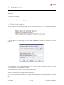
7. Databases ..............................................................................................................................
7.1. Connection to a CSV file ...................................................................................................
7.1.1. Form of the database ...................................................................................................
7.1.2. Connection ................................................................................................................
7.2. Connection via a JDBC link (example with ODBC connector) ...................................................
7.2.1. Form of the database ...................................................................................................
7.2.2. Connection ................................................................................................................
7.3. Operation .........................................................................................................................
59
59
59
59
60
60
60
61
8. File
8.1.
8.2.
8.3.
8.4.
8.5.
8.6.
Saving ............................................................................................................................
Model .............................................................................................................................
Petri Net model ................................................................................................................
RTF File ..........................................................................................................................
Input data ........................................................................................................................
Results ............................................................................................................................
Curves .............................................................................................................................
63
63
63
64
64
64
66
9. Options of GRIF - Stochastique Block Diagram ........................................................................
9.1. Executables ......................................................................................................................
9.2. Database ..........................................................................................................................
9.3. Language .........................................................................................................................
9.4. Options ...........................................................................................................................
9.5. Graphics ..........................................................................................................................
9.6. Digital format ...................................................................................................................
9.7. Blocks .............................................................................................................................
9.8. Repeated blocks ................................................................................................................
9.9. Connectors .......................................................................................................................
9.10. Curves ...........................................................................................................................
67
67
67
67
67
68
68
68
68
69
69
User Manual
3 / 69
Version 31 March 2014
1. Description of the interface
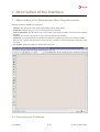
1.1. Main window of the Stochastique Block Diagram module
The main window is divided into several parts:
• Title bar: The title bar shows the names of the module and file being edited.
• Menu bar: The menu bar gives access to all the application's functions.
• Icon bar (shortcuts): The shortcut bar is an icon bar (horizontal) which gives faster access to the most common
functions.
• Tool bar: The tool bar (vertical) allows you to select the elements for modeling.
• Input zone: A maximum amount of space has been left for the graphical input zone for creating the model.
• Tree: A tree is "hiden" between input zone and tool bar. It enables to walk through pages and groups of the
document.
• Set of tables: Tables are gathered in "hiden" tabs on the right.
1.2. Description of the Menus
User Manual
4 / 69
Version 31 March 2014
1. The File menu contains the standard commands used in this type of menu (open, close, save, print, etc.). The
properties (name, creation date, created by, description, version) can be accessed and modified by selecting
Document properties. The Document statistics provide information on the model's complexity. It is also
possible to access a certain number (configurable) of recently modified files.
The icon bar just under the menus proposes shortcuts for most of the File commands:
2. The Edit menu contains all the commands needed to edit the model being input graphically.
The icon bar just under the menus proposes shortcuts for most of the Edit commands:
3. The Tools menu contains all the commands needed to manage the current model (page management,
alignments, options, etc.).
User Manual
5 / 69
Version 31 March 2014
The icon bar just under the menus proposes shortcuts for most of the Tools commands:
4. The Document menu gives access to all the documents being created or modified.
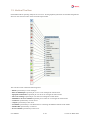
5. The Block Diagram menu contains all the commands needed to produce the graphical part of the current model.
The vertical icon bar on the left of the application provides shortcuts for each of the Block Diagram commands
(cf. vertical tool bar).
User Manual
6 / 69
Version 31 March 2014
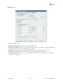
6. The Data and Computations menu is divided into two parts: data management (creation and management of
the different parameters) and configuration/computation launch (computation time, desired computation, etc.)..
NB: The Verify function detects any errors in the model: data without values (equal to NaN), places with an
identical number, etc.
7. The Group menu concerns the input and management of submodels grouped into independent subassemblies.
The icon bar just under the menus proposes shortcuts for two of the Group commands:
8. Finally, the Help menu accesses the on-line Help, the Help topics and to "About".
User Manual
7 / 69
Version 31 March 2014
1.3. Vertical Tool bar
Each model used for operating safety has its own icons. All the graphical symbols for the stochastic diagrams are
shown on the vertical icon bar on the left of the input window.
The vertical tool bar contains the following items:
•
•
•
•
•
•
•
•
•
•
Block represented by a brown rectangle.
Bloc en bibliothèque représenté par un livre sur un rectangle de couleur brune.
Equipe de maintenance représenté par une clé sur un rectangle de couleur brune.
Pièces de rechange représenté par une valise sur rectangle de couleur brune.
Défaillances de cause commune représenté par un éclair sur un rectangle de couleur brune.
Connector represented by a brown arrow.
Output represented by a blue arrow.
Serial link represented by a non-directional arc connecting the different elements of the model.
Divider link represented by a red arrow.
K out of N link represented by a blue arrow.
User Manual
8 / 69
Version 31 March 2014
•
•
•
•
•
•
Identical block represented by a pink dotted block.
Input represented by a red arrow.
Sourcerepresented by a green circle.
Target represented by a yellow circle.
Resource block creates an "independent" block represented by a green and yellow rectangle.
Negation (only accessible in Reliability diagram mode) reverses the block's logic and adds a sort of cross
inside the rectangle.
• Comment to add text directly on the chart.
• Dynamic display to display a value of a model element.
• Charts to draw curves representing computations on the model.
1.4. Data Editing Tables
1.4.1. Description of the Tables
To create or modify data (parameters, variables, etc.), tables are available in the Data and Computations menu
and in tabs at the right of the view. All the GRIF 2014 data tables operate in the same manner.
The data editing table/panel is divided into 3 parts:
• The top part containing the buttons.
• The main part containing the data table.
• The bottom part indicating what the selected data is used for.
Saves the table in a text file.
Opens the table in a text editor (that defined in the Options).
Opens the column manager.
When the display selection button is pressed, a click in the table leads to the selection in the input
area.
Displays the data filtering part.
Multiple modifications made to all the selected data.
Creates new data.
Duplicate the selected data (ask a new name)
Deletes the selected data (one or many).
Enables data filtering or not.
User Manual
9 / 69
Version 31 March 2014
Defines the filter to be applied to the data.
Filtering allows you to display only what is necessary in a table. Several filtering criteria can be combined, as
shown below:
Select AND or OR to choose the type of association between each line (filter criterion). A line is a Boolean
expression divided into 3 parts:
1. the first is the column on which the filter is used;
2. the second is the comparator;
3. the third is the value to which the data will be compared.
If the Boolean expression is true, the data will be kept (displayed); otherwise the data will be masked. When the
filter is enabled its value is displayed between < and >.
The data in a column can be sorted by double clicking the header of this column. The first double click will sort
the data in ascending order (small triangle pointing upwards). The second double click on the same header will
sort the column in descending order (small triangle pointing downwards).
A table can contain many columns, some columns may be unnecessary in certain cases. The "linked to database"
column is unnecessary when no database is available. It is thus possible to choose the columns to be displayed
and their order. To do this, click right on a table header, or click the Columns Manager button, the following
window opens:
You can choose the columns to be displayed by selecting (or deselecting) the corresponding check boxes. The
arrows on the right are used to move the columns up or down in the list to choose the order of the columns. The
Disable data sorting check box disables the data sorting. This improves the application's performance with very
complex models.
To modify data, double click the box to be modified. When several lines are selected (using the CTRL or SHIFT
keys) changes can be made to all the selected data by using Multiple changes. A window then opens to allow
you to make these changes.
User Manual
10 / 69
Version 31 March 2014
Items which cannot be modified are greyed. The white lines indicate that the selected data does not have the same
value for the field in question. A new value can be entered which will be taken into account for all the selected
data. The lines with no background colour indicate that all the selected data has the same value for this field (in
this example the selected data is all "Float"); they can be changed to give a new value to all the selected data.
The bottom table in the data table indicates which elements in the model use the selected data. The first column
of this table gives the name of these elements; the second indicates their location in the document (page, group).
Clicking on a line in this bottom table opens the page where the element is located and selects the element.
1.4.2. Table accessibility
As mentioned above, the tables can be accessed via the Data and Computations menu; in this case, each table
is displayed in a separate window.
To avoid having too many windows open, all the tables are grouped together in tabs on the right-hand side of the
application. This area can be hidden/displayed using the small arrows above the input zone.
It is possible to choose the tables in this zone by right clicking on the tabs. A contextual menu appears, in which
the user can select the tables s/he wishes to display.
1.4.3. Data creation
The Parameter editor is used to create "boolean", "integer" and "real" parameters. The following window is
used to choose the name, domain and value of the new parameter. Its value must be entered later directly in the
parameter table.
User Manual
11 / 69
Version 31 March 2014
The Parameter editor is used to create variable defined with complex expression. Creation is made with the same
window as parameter editor.
When variable is created, a double click in definition part opens code editor.
The code editor has three parts. The first is an editable text zone where you enter the code using Moca-RP syntax.
Under this zone is a noneditable zone indicating any errors which may arise. The third is the Tools part which
is a data entry aid.
The Syntax button makes a syntax change. The Semantics button checks the semantics. The errors are displayed
in the bottom left part. Under the buttons there are drop-down menus giving access to the model's various data.
Select the desired data then click the <= button to insert it in the code.
The Functions drop-down menu shows funtions that can be used in Moca (cf Moca User Manual).
The third menu display function that are available in MocaAdd.dll, for more information (cf Moca12 user manual)
A parameter can be transformed into variable and vice versa, by right-clincking on it and selectiong Change to
variable ou Change to paramètre
User Manual
12 / 69
Version 31 March 2014
1.5. Tree view
To help users to walk through the document (pages, groups ans sub-groups), a tree is available on the left of the
application. By default, every element is displayed, you can use Filter button in order to select elements you want
to display or not.
You can expand or collapse a node in a recursive way with a right click on the node.
As explained for tables on the right, you can "hide" the tree.
User Manual
13 / 69
Version 31 March 2014
2. Creating a stochastic diagram
2.1. Entering the diagram
2.1.1. Type of diagram
When a new document is created, you can choose between two working modes:
1. Reliability diagram: allows you to work in Boolean logic ("work/failed" or "1/0" logic).
2. Flow chart: allows you to work with real flows and capacities for each block.
NB: The difference between the two modes mainly resides in the type of prototypes available and in the way the
computations are performed.
2.1.2. Entering the blocks in the library
First of all, it is possible to select the prototype used by default when creating the blocks. Just right click on the
Library Block icon on the vertical tool bar and select the appropriate prototype in the list.
To input the various Blocks, select the corresponding symbol in the vertical tool bar. Then each click left on the
graphical input zone will create a new element. Each of the model's blocks is characterised by three parameters:
1. A number: Located in the centre of the blocks, they are automatically incremented. These numbers are the
true identifiers of the blocks which will be used by the computation engine. That is why two blocks cannot
have identical numbers.
User Manual
14 / 69
Version 31 March 2014
2. A name: A default name is assigned to each block ("Bi" for block number "i"). Since each block normally
represents a precise component or a subsystem, you are strongly recommended to assign it a more mnemonic
name than that given by default. This enables you to locate yourself better in the model and in the results file.
3. A prototype: : it is the name of the prototype which is "behind" the block. Each block in the diagram hides a
prototype representing a "standard component", created using the Petri12 module (cf. document on prototypes).
2.1.3. Entering standard blocks
Another way to use stochastic diagram consists inf use predefined blocks. There are 4 types of block available:
•
•
•
•
Bloc: stand for complete component.
Maitenance Team: stand for repair team.
Spare parts: stand for spare parts.
Common cause failure: stand for common cause failure.
2.1.3.1. Complete Block
Complete block is used for modeling component easily.
In order to create a complete block, select Bloc symbol on vertical tool bar, or in menu. A new element is then
created whenever you click left on the graphical entry area.
The configuration of the block can be edited by right clicking on the symbol of the block previously created in
the graphical entry area.
A multi-tab window is used to configure the block.
User Manual
15 / 69
Version 31 March 2014
Prototype description tab:
It contains informations on the prototype.
• Name: Prototype name.
• Id: Prototype identifier.
• Use specific picture for this bloc: enables to change picture of the block. Just check the box and choose picture
using
button.
• Maximum capacity: Maximum capacity in nominal mode. This property is only available for flow-diagrams.
Onglet Main characteristics:
It contains main characteristics of prototype.
• Failure type: failure type (Revealed failure, Hiden failure, Hiden failure + Revealed failure, Critical
failure, Critical failure + Degraded failure).
User Manual
16 / 69
Version 31 March 2014
• Initial state of prototype: Combo-box enables you to select initial state of component : Work, Failure or
others (depending on failure type).
• Spare parts management: Enables to select a stock of spare parts to be used for repairs. Stock can be selected
in combo-box, or created thanks to
button.
• Preventive maintenance: Enables to activate the definition of preventive maintenance. This option is only
available if there is at least a critical failure.
• Standby: Enables to activate the definition of standby state.
• Start condition(s): necessary condition(s)condition(s) leading to exit standby state. The condition is editable
in the textfield, or you can use formula editor using
button.
• Fail to start probability: probability that component fails during standby exit. In order to activate this
probabilty, check the box and enter a Gamma.
• Law and Parameters: law ruling failures during standby states.
• Use repair team: enables to select a repair team, Enables to select a repair team to be used for repairs. Teams
can be selected in combo-box, or created thanks to
button.
Revealed failure tab:
It contains revealed failure setup.
• Definition of revealed failure: definition of law ruling revealed failures.
• Common cause failure: Enables to activate common cause failures by checking box. Common cause failure
can be selected in combo-box, or created thanks to
button.
• Repairable: Enables to specify if revealed failure is repairable. In this case, repair must be set-up.
• Law and Parameters: law ruling repair.
• Use repair team: Enables to select a team to be used for repairs. Teams can be selected in combo-box, or
created thanks to
button.
User Manual
17 / 69
Version 31 March 2014
Hiden failure Tab:
It contains hiden failure setup.
• Definition of hiden failure: definition of law ruling hiden failures.
• Common cause failure: Enables to activate common cause failures by checking box. Common cause failure
can be selected in combo-box, or created thanks to
button.
• Repairable: Enables to specify if revealed failure is repairable. In this case, repair must be set-up.
• Test type and Paramètres: define the way hiden failure component is tested and repaired.
• Use repair team: Enables to select a team to be used for repairs. Teams can be selected in combo-box, or
created thanks to
button.
User Manual
18 / 69
Version 31 March 2014
Critical failure tab:
It contains critical failure setup.
• Definition of critical failure: definition of law ruling critical failures.
• Common cause failure: Enables to activate common cause failures by checking box. Common cause failure
can be selected in combo-box, or created thanks to
button.
• Repairable: Enables to specify if critical failure is repairable. In this case, repair must be set-up.
• Law and Parameters: law ruling repair.
• Use repair team: Enables to select a team to be used for repairs. Teams can be selected in combo-box, or
created thanks to
button.
User Manual
19 / 69
Version 31 March 2014
Degraded failure tab:
It contains critical degraded setup.
• Definition of degraded failure: definition of law ruling the way component fails (degraded mode).
• Degraded mode capacity: Capacity of component when it is in degraded mode. This property is only available
for flow-diagrams.
• Transition to critical state: definition of law ruling the way compoent fails from degraded mode to critical
mode.
• Repairable: Enables to specify if critical failure is repairable. In this case, repair must be set-up.
• Repair condition: definition of the condition for degraded failure reparing. The condition is editable in the
textfield, or you can use formula editor using
button.
• Law and Parameters: law ruling repair.
Preventive maintenance Tab:
User Manual
20 / 69
Version 31 March 2014
It contains setup of preventive maintenance for component.
•
•
•
•
Maintenance type: preventive maintenance type.
Maintenance frequency: frequency of each maintenance type.
Maintenance duration: duration of each maintenance type.
Maintenance start condition: definition of condition to start preventive maintenance. The condition is editable
in the textfield, or you can use formula editor using
button.
• Maintenace team selection: Enables to select a team to be used for repairs. Teams can be selected in combobox, or created thanks to
button.
2.1.3.2. Blocks of Ressources
There are 3 type of ressource-block:
• Maitenance Team.
• Spare parts.
• Common cause failure.
In order to create a Maitenance Team, Spare parts or Common cause failure, select associated symbol on
vertical tool bar, or in menu. Then each click left on the graphical input zone will create a new element. Another
way consists in using tables. Selct tabs of the ressources you want to add, and click on Add button :
.
• Maitenance Team:
• Spare parts:
User Manual
21 / 69
Version 31 March 2014
• Common cause failure:
You can edit block configuration by right-clicking on block left on the graphical input.
2.1.3.2.1. Maitenance Team
•
•
•
•
•
•
•
•
•
Name: Name of Maitenance Team.
Number: Id number of Maitenance Team.
Repairer count: Number of repairer in team.
With mobilization: specify if the team must be mobilized.
Mobilization time: time needed by the team to start repairing.
Repair after Xth failure: Number of failures for equipments before team must step in.
With time slot: Used if maintenance team is not always available (has time slot) to repair failures.
Start hour: Time slot beginning.
Stop hour: Time slot ending.
User Manual
22 / 69
Version 31 March 2014
2.1.3.2.2. Spare parts
•
•
•
•
•
•
•
Name: Name of Spare parts.
Number: Id number of Spare parts.
Initial stock: Number of spare parts in initial stock.
Supply: Type of supply for spare parts (None, Periodic, On demand).
Stock after restocking: Number of spare parts in stock after supply.
Supplying threshold: Size of stock from which supply is asked (only available with supply on demand).
Supplying delay: Delay needed for full restocking when threshold is reached (only available with supply on
demand).
• Fisrt supply: date of fisrt supply (in hours) (only available with periodic supply).
• Duration between supplies: duration between 2 re-stocking (in hours) (only available with periodic supply).
2.1.3.2.3. Common cause failure
• Name: Name of Common cause failure.
• Number: Id number of Common cause failure.
• Law and Parameters: definition of law ruling common cause failure.
2.1.4. Inputting links and connectors
LINKS
• Function: directly links two elements (block or connector).
• Graphical representation: a non-directional arc.
• Creating a link:
User Manual
23 / 69
Version 31 March 2014
1. select the corresponding icon on the vertical tool bar;
2. select a start element (block or connector) by a click left on it;
3. drag the mouse (without releasing the button) to the arrival element and release the button.
The order in which the links are drawn can in some cases have an importance (cf. below).
• Example:
In the above example, two serial links have been drawn: one between blocks B1 and B3 then the other between
B2 and B4.
CONNECTORS
• Function: this element can be the "source" and "target" of several links.
• If it is the "Source" of several links, it is called a divider connector.
• If it is the "Target" of several links, it is called a K out of N connector.
• Graphical representation:
• the "conventional" connectors are brown triangles;
• the divider connectors are red triangles;
• the K out of N connectors are blue triangles.
Important NB: Depending on the links which are linked to the connector, it is automatically converted into a
divider connector or into a K out of N connector.
• identification: each connector has
• a number: It is the "true" identifier (that which will be used by the computation engine). The numbers are
automatically incremented. Two connectors cannot have an identical number.
• a name: allows you to give the connector a name to locate yourself better in the model.
• a number K (only for K out of N connectors): This number is equal to the number of input links which must
supply a positive message so that the output link has a positive message.
• Operation:
To create a "conventional" connector,
1. select the corresponding icon on the vertical tool bar;
2. click left at the desired location in the input zone.
divider or K out of N connectors can be created directly. To do this
1. select the corresponding icon on the vertical tool bar;
2. select a start element (block or connector) by a click left on it;
3. drag the mouse (without releasing the button) to the arrival element and release the button.
User Manual
24 / 69
Version 31 March 2014
• Example:
In the example above, a divider connector has been drawn between blocks B1 and B3 and a K out of N connector
has been drawn between B2 and B4.
The connectors can be created automatically by creating links between the different elements. Here are some
examples to help you understand how this works:
• Let B1, B2, B3 and B4 be four blocks.
• If a link is drawn between B1 and B2 followed by another between B1 and B3, then a divider connector is
automatically created.
User Manual
25 / 69
Version 31 March 2014
• If a link is drawn between B2 and B4 followed by another between B3 and B4, then a K out of N connector
is automatically created (with K equal to 1).
• To check that a connector with several inputs and several outputs becomes a conventional connector again,
draw a link between B4 and connector C1.
NB: To link new components to B4 (for example), the "target" of the link can be either block B4 or connector C2.
Care must be taken when creating automatic connector since the direction of the links created is very important.
2.1.5. Separator Connector (flow diagram)
2.1.5.1. Choose connector type
Separator-connectors are connectors whose output is not equal to input. To use separator type, right-click on
connector and select Type of connector / Separator connector.
2.1.5.2. Set-up Separator Connector
When editing Separator Connector, the following window is displayed.
For each output (here : one to C2, one to B3, one to B1), you can choose a factor which will be used to compute
output value. Let factori be a factor linked to Si output, then Si = Input / Reference * factori.
2.1.6. Source and Target blocks
Each model must have at least one Source block and one Target block.
NB: In the case of a reliability diagram, there can be several "Sources" and/or several "Targets. In the case of a
flow chart, there can only be a single "Source" and only a single "Target" (due to the computation method).
• Sources must be placed at the start of the diagram, it is impossible to create links directed to them.
User Manual
26 / 69
Version 31 March 2014
• Targets must be placed at the end of the diagram, it is impossible to create links leaving from them.
To create these two types of blocks:
1. select the corresponding icon on the vertical tool bar;
2. click left on the desired location in the input zone.
Example:
NB: The availability and reliability computations will be performed at "Target" block level
2.1.7. Resource blocks
Certain prototypes in the library are used to model events "parallel" to the model: the common mode failures
("CCF" prototype), the mobilisations and demobilisations of the intervention supports ("MobilK" prototype), etc.
The blocks using this type of prototype have no place in a functional diagram's logic but, however, must be taken
into account in the computations.
To clearly specify that this type of block must be considered in the computations, they must be defined as "Resource
Blocks". To do this, select the corresponding icon on the vertical tool bar then click on the block concerned.
NB: The availability and reliability computations will be performed at "Resource" block level in addition to the
"Target" blocks (Cf. options to desactivate ressource computation).
2.1.8. Negation function
This function is only available for flow charts. It is used to reverse a block's logic.
To apply a "Negation" to a block:
1. select the corresponding icon on the vertical tool bar;
2. click left on the block concerned.
NB: the "Negation" is not accessible in flow chart editing mode.
User Manual
27 / 69
Version 31 March 2014
2.1.9. Entering Comments
To add a comment anywhere on the chart, click the pencil icon and place yourself on a point in the graphical input
zone. The Comment dialogue box opens where you can enter the desired comment.
Note: Character "%" is a reserved character, it must be type twice "%%" in order to display "%".
2.1.10. Dynamic fields
It may be useful to observe the change in the different parameters of the model. It is also usefull to see a result
next to its corresponding system. To do this, use dynamic fields by selecting the corresponding icon on the vertical
tool bar:
The dynamic fields are a type of "improved comments". They can be used not only to enter words or phrases but
also to insert model values or results.
If you want to display informations about a data of the model, you must use the following syntax:
$data.'type of data'.'field used o search data'('value that the field must match).'information you want to display
for the selected data'
We can analyze the above windows as follows: I am looking for a "parameter" which "name" is 'lambda", and I
want to display its "value". When you type the first letters, a completion system helps to type script without error.
If you want to display a result of the result-bank, the syntax is the following:
User Manual
28 / 69
Version 31 March 2014
$result.bank('path in the bank').target('target result').'what you want to display'.'at what time'
We can analyze the next picture as follows: I am looking for a result which path in the bank is "default-Moca", I
want results for "TS3 for 'available' valriable" and I want its value for the "last" time. If last is replaced by time(10)
we obtain value at t=10.
You can also display a summary of result. Replace 'what you want to display' by summary. In this case, summary
is the last word of this script.
A button has been added in 2013 version, it is a script generator for model data.
2.2. Configuring the Elements
All the graphical elements can normally be edited with a double-click on them or using the Edit - Properties
menu, or using the shortcut Alt + Enter.
2.2.1. Configuring the blocks
When you click right on a block you have the choice between
• changing the prototype (selecting another prototype in the library);
• modifying the properties and configuring the element from the prototype.
This window has four tabs which are used to modify the properties.
2.2.1.1. General tab
This tab is the first to appear. It allows you to:
• enter the block name;
• change the number;
• select the initial state;
User Manual
29 / 69
Version 31 March 2014
• read all the comments.
2.2.1.2. Transitions tab
This tab is used to configure all the prototype's transitions which were defined as external. They are listed in a
two-column table. To modify the transition laws:
• double click in the right hand column;
• select a law;
• configure the law.
NB: The model's parameters can be accessed to use them for the transition law level.
2.2.1.3. Places tab
This tab is used to link the prototype's external places to model places. The places under BStoK are not shown
graphically. They are only used to set up connections with the prototypes. For each place in the table:
• double click in the right hand column;
• enter the number of the place in the model to which it will be connected;
• press the Enter key on the keyboard to validate the selection.
NB: No computation can be launched if unconnected places still remain.
2.2.1.4. Variables tab
This tab links the prototype's external variables to model variables. For each variable in the table:
• double click in the right hand column;
• select one of the model's variables using the code editor;
• click OK to validate the selection.
User Manual
30 / 69
Version 31 March 2014
NB: No computation can be launched if unconnected variables still remain.
NB2: Let "varInPrototype" a variable which is modified inside prototype, it can not be linked to a variable of the
document with a complexe definition. Let "var" be a variable of the document with complex definition : var =
var2 * 2, it would be a nonsense to liked "varInPrototype" to "var". If there is a transition with an assignment
"varInPrototype" = 3 inside prototype, it would become "var" = 3. Obviously "var" can't be equal to 3 and equal
to "var2" * 2 !
2.2.1.5. Parameters tab
This tab allows you to give a value to the prototype's external parameters. For each parameter in the table:
• double click in the right column;
• select one of the model's parameters form the drop-down list OR directly enter a value;
• press the Enter key on the keyboard to validate the selection.
NB: The use of prototypes in the BStoK module and all the connection problems are covered in greater detail in
the document on prototypes.
2.2.2. Configuring the connectors
You can modify any of a connector's parameters:
• change the name and/or the number for the divider connectors and the "conventional" connectors;
• change the name, number and/or value of K for the K out of N connectors.
NB: In the case of a number modification, it is important to keep in mind that two connectors cannot have the
same number.
User Manual
31 / 69
Version 31 March 2014
2.3. Example of stochastic diagram
Here is a stochastic diagram modeling the behaviour of any system for which only two repair teams are available.
The above diagram has nine blocks:
• Comp1
• Number: 1
• Prototype: Mod2
• Initial state: "Work"
• Transitions: Failure is an exponential law of parameter Lambda_A and Repair Repair is an exponential law
of Mu(the other transitions keep their default laws)
• Variables: Nbrep is connected to Nbrep_system
• Parameters: gamma takes the value G, and NK takes the value NK1
• Comp2
• Number: 2
• Prototype: Mod2Test
• Initial state: "Work"
• Transitions: Failure is an exponential law of parameter Lambda_B and Repair Repair is an exponential law
of Mu(the other transitions keep their default laws)
• Variables: Nbrep is connected to Nbrep_system
• Parameters: gamma takes the value G, and NK takes the value NK2
• Comp3
• Number: 3
• Prototype: Mod2Test
• Initial state: "Work"
• Transitions: Failure is an exponential law of parameter Lambda_B and Repair Repair is an exponential law
of Mu(the other transitions keep their default laws)
User Manual
32 / 69
Version 31 March 2014
• Variables: Nbrep is connected to Nbrep_system
• Parameters: gamma takes the value G, and NK takes the value NK3
• Comp4
• Number: 4
• Prototype: Mod2Test
• Initial state: "Failed"
• Transitions: Failure is an exponential law of parameter Lambda_B and Repair Repair is an exponential law
of Mu(the other transitions keep their default laws)
• Variables: Nbrep is connected to Nbrep_system
• Parameters: gamma takes the value G, and NK takes the value NK4
• Comp5
• Number: 5
• Prototype: Mod2Test
• Initial state: "Work"
• Transitions: Failure is an exponential law of parameter Lambda_B and Repair Repair is an exponential law
of Mu(the other transitions keep their default laws)
• Variables: Nbrep is connected to Nbrep_system
• Parameters: gamma takes the value G, and NK takes the value NK5
• Comp6
• Number: 6
• Prototype: Mod2Test
• Initial state: "Work"
• Transitions: Failure is an exponential law of parameter Lambda_B and Repair Repair is an exponential law
of Mu(the other transitions keep their default laws)
• Variables: Nbrep is connected to Nbrep_system
• Parameters: gamma takes the value G, and NK takes the value NK6
• Comp7
• Number: 7
• Prototype: Mod1
• Initial state: "Work"
• Transitions: Failure is an exponential law of parameter 2.5e-5
• Variables: Nbrep is connected to Nbrep_system
• Parameters: NK takes the value NK7
• Comp8
• Number: 8
• Prototype: Mod2
• Initial state: "Failed"
• Transitions: Failure is an exponential law of parameter Lambda_A and Repair Repair is an exponential law
of Mu(the other transitions keep their default laws)
• Variables: Nbrep is connected to Nbrep_system
• Parameters: gamma takes the value G, and NK takes the value NK8
• Comp9
• Number: 9
• Prototype: Mod2
• Initial state: "Work"
• Transitions: Failure is an exponential law of parameter Lambda_A and Repair Repair is an exponential law
of Mu(the other transitions keep their default laws)
• Variables: Nbrep is connected to Nbrep_system
• Parameters: gamma takes the value G, and NK takes the value NK9
Five connectors :
• Div1
• Number: 1
User Manual
33 / 69
Version 31 March 2014
• Type: divider
• Conv1_Div2
• Number: 2
• Type: K out of N and divider
• Value of K: 2
• Conv2
• Number: 3
• Type: K out of N
• Value of K: 1
• Div3
• Number: 4
• Type: divider
• Conv3
• Number: 5
• Type: K out of N
• Value of K: 1
A "Source" block:
• Name: "in"
• Value of NK: 100.0
A "Target" block:
• Name: "out"
• Value of NK: default value
In this example most of the laws which have been used are exponential laws and Dirac laws. However, any other
type of law could have been used (e.g.: log-normal law for the repair transition). Also, the presence of Dirac laws
has enabled us to mix the deterministic phenomena and the random phenomena.
This diagram, produced in only a few minutes, models (based on Petri nets) several more or less complex
components: repairable, not repairable, regularly tested, etc. (all of which is under a constraint of a limited number
of repair teams).
Through this example we can see that the BStok module combines:
• flexibility of the Petri nets (due to the exhaustiveness of the list of available prototypes);
• fast input
NB: The prototype library can be modified or completed to increase the modelling power (cf. document on
prototypes).
2.4. Using Shortcuts
2.4.1. Shortcuts to the connectors
The concept of a shortcut (or repeated element) was introduced in the Stochastique Block Diagram module for
four main reasons:
•
•
•
•
To link together portions of the model;
To avoid graphicaly complex model, and keep readability;
To simplify the use of the Group function (cf. below);
To highlight what is essential and what is not.
User Manual
34 / 69
Version 31 March 2014
Let two blocks Sys1 and Sys2 connected by single link: lien:
A shortcut link is created in several stages:
1. Delete the existing link.
2. Create an Output and draw a link between Sys1 and this Output.
3. Create an Input connector relative to the Output (by a click left on the corresponding icon in the vertical tool
bar then by clicking on the Output).
4. Finally, draw a link between the Input connector and Sys2.
The Output connector (shown in blue) has a name and number whereas the Input connector (shown in red) only
has the number of the Output to which it is linked.
Although linked from the "computational logic" viewpoint, the two blocks are now graphically completely
independent. They can now be placed on different pages or in different groups (cf. below).
User Manual
35 / 69
Version 31 March 2014
2.4.2. Shortcuts to blocks or duplicate blocks
From the logic viewpoint a block can have an "impact" on several parts of a same diagram. To correctly model
this case this block must be duplicated. To do this, select the corresponding icon, in the vertical tool bar then click
the block to be duplicated:
The block which has just been duplicated is now marked by a double line contour whereas the duplicated block
is shown in pink with a dotted contour.
The centre of the duplicated block displays its own number and the number of the original block. And the following
appear below the block:
• the name of the original block preceded by "Ref=",
• the name of the duplicated block,
• a comment, where necessary.
The number, name and comment can be modified by a click right:
You now just have to insert the duplicate block in the model, and at each instant its status will be equal to that
of the original block.
Note: if the original block is deleted then the repeated block is also deleted.
2.5. Page and group management
The use of shortcuts allowed us to obtain two Block Diagram which have no graphical link between them. They
communicate only by shortcuts. This can be used, for example, to place each subpart on a different page:
1. Create a new page by clicking the corresponding icon in the icon bar (or use menu Tools - New Page). A page
number 2 is thus created.
2. Return to page 1 by selecting the page using the page selector in the ideographic command bar (or use menu
Tools - Page manager).
3. Select the part to be moved.
4. Open menu Tools - Change page.
5. Select page 2 and click OK. The part selected is transferred to page 2 but it continues to communicate with
page 1 via the shortcuts.
Note: For large models the division method described above is very useful.
User Manual
36 / 69
Version 31 March 2014
Another possibility for entering large Block Diagram is to use the Group concept. This is made possible by the
shortcuts and the fact that the data is global for a document. This allows quite separate subparts to be created:
1. Select a subpart.
2. Use menu Group - Group. A dialogue box then opens asking for the name to be given to the group being
created.
3. Enter the desired name and click OK (e.g.: "System 1"). The group is created: the subnet is replaced by a
rectangle assigned with the chosen name.
You can also create an empty group with Group - New Group menu or group tool in the left toolbar.
Each group can then be edited, renamed or ungrouped using the commands in the Group menu. The group can
also be edited with a click right or using the "cursor down arrow" on the left of the page manager. In Edit mode,
the submodel can then be modified as you wish. When the modification is terminated you return to the previous
figure by exiting group editing by menu Group - Quit Group Edition, or using the "cursor up arrow" on the left
of the page manager. It's also possible to choose a picture for a group by using Group - Change Picture menu.
Note: Groups can be grouped recursively.
2.6. Sub-systems creation
In some cases it may be useful to group part of the diagram which involves breaking the links. To do this, use the
Break and Group function. This is what the result could be for a simple example:
User Manual
37 / 69
Version 31 March 2014
The above figures show how the different shortcuts have been arranged. For each "broken" link, an Output
connector and its corresponding Input have been automatically created. This mechanism has allowed the selected
part to become a sub-system.
You can create sub-systems with the Group menu, or with a right-clic on the page. By default, a sub-system
consists of an input connector, an output connector, and a "group" in which one the behavior of the sub-system
is discribed.
Inputs or outputs can be added or deleted doing a right-clic on the sub-system.
Connector deletion is made with thanks to this window :
User Manual
38 / 69
Version 31 March 2014
Before being deleted, a connector must not be linked to another node (neither in the sub-system, nor outside).
2.7. Data Entry Aids
To simplify model creation the Stochastique Block Diagram module has different data entry aids to automate timeconsuming operations.
2.7.1. Copy / Paste / Renumber (without shortcut)
To assist with the entry of the repeated parts of the Block Diagram "Copy / Paste and Renumber" mechanisms
have been provided. This operation is carried out in 6 steps:
1.
2.
3.
4.
5.
6.
Select the part to be copied.
Click the Copy icon, or use menu Edit - Copy or the shortcut Ctrl + C.
Click the Paste and Renumber icon, or use menu Edit - Paste and Renumber or the shortcut Ctrl + R.
A window appears where you choose the start number for the renumbering.
The previously selected part is copied and the copy is selected.
Move the copy to the desired location.
We then obtain the diagram shown in the figure below:
• Blocks 1,2,3 and 4 of diagram are became 5,6,7 and 8 for the copy;
• Connectors C1 and C2 are became C3 and C4 for the copy.
User Manual
39 / 69
Version 31 March 2014
When copying to a new document, any data conflicts are handled in the following window:
This window shows all the data which has the same name in the source document and the destination document.
There are three choices:
1. Use data of destination document, this will replace the occurrences of the data in the source document by the
data with the same name in the destination document.
2. Create a copy for each data in conflict, this will replace the occurrences of the data in the source document by
a copy with a name with the suffix "copy".
3. Manually manage conflict, this allows you to choose whether you use the existing data or not, depending on the
data. You can also specify the name of the copy by double clicking on the box in the "destination document"
column. The names in this column are normally masked when the Use existing check box is selected, since it
is the data which is already in the destination document which will be used.
2.7.2. Copy / Paste / Renumber (with shortcut)
The "Copy / Paste and Renumber" command creates new "instances" i.e. new subcharts similar to the sub-diagrams
copied:
• Same graphical structure;
• Same prototypes used;
• Same parameters;
• The block number and names change (new name: Bi, where i is the new number);
• The connector numbers change but not their names.
User Manual
40 / 69
Version 31 March 2014
When Output connectors are part of the selection to be copied / pasted and renumbered, they will then also be
renumbered.
In the above example, Ouput C7, C9 and C11 have been renumbered.
NB: Also, this example enables us to check the five points mentioned previously.
When Input connectors are part of the selection to be copied / pasted and renumbered, then they will remain linked
to the same Ouput connectors if these connectors are not part of the selection.
In the above example, the Inputs are always linked to the same Ouput connectors.
When Input connectors (and their corresponding Ouputs) are part of the selection to be copied / pasted and
renumbered, they will then be connected to the new Output connectors
In the above example, the Inputs are renumbered, so Ouput connectors are also renumbered.
You can navigate between an element's different shortcuts, using menu Tools/Navigate to shortcuts. A window
opens and displays the list of shortcuts. Clicking on a shortcut automatically positions the view on this shortcut.
You can return to the original element by clicking on its name at the top of the window.
2.7.3. Ordinary Copy/Paste
In addition to the "Copy / Paste and Renumber" command there is an ordinary "Copy / Paste" function. It is used
to make a single copy without renumbering. We thus obtain double elements which, from a formal viewpoint, is
incorrect but which must be temporarily tolerated to simplify data entry.
User Manual
41 / 69
Version 31 March 2014
Where possible, the "Copy / Paste and Renumber" function must be used in preference to the simple "Copy / Paste"
function to minimise the risk of errors. But when it is used you must take the necessary precautions to re-establish
the correct numbering to eliminate the duplicates.
2.7.4. Overall change
When creating the Block Diagram it may be necessary to change a large part of the elements in the models:
changing the names, numbers, etc. The "Replace all" function in the Edit menu allows you to perform overall
changes:
• Use the Edit / Overall changes function.
• Choose the type of elements to be modified among available tabs.
• The "Find / Replace" part changes a character string present in one or more variable labels, place labels or
transition labels. It is replaced by the string entered in the "Replace" part.
• The "Renumber" part only concerns the places. It is used to change place numbers. You indicate a Start number
then specify a constant Step, or Add a constant value to the current numbers.
• Click OK to return to the chart. The changes are validated.
Note: The name changes and renumbering can be done manually if the necessary precautions are taken (avoiding
duplicates, etc.). You click the Future number or Future name column and enter the change. Do not forget to
validate it with the "ENTER" key.
2.7.5. Selection change
The "Replace selection" function is equivalent to a "Replace all" but only applied to the selected elements. Only
the selected blocks and connectors can be replaced.
NB: The "Replace selection" function does not allow the model's parameters to be replaced.
User Manual
42 / 69
Version 31 March 2014
2.7.6. Document properties / Images management
File - Doucument properties menu enable to save information about document : name, version, comment, ...
These informations are available in General tab.
Images may be very useful to represent sub-system. GRIF 2014 enables to save images that can be used in different
parts of software (groupes, prototypes, ...). Images management is made in Images tab.
To add a new picture into document, use
icon. A double click in File column enables to select an picture (jpg,
gif or png). A double click in Description column enables to give a name or a description to selected image.
Once in document, picture can be linked to a groupe with Group - Picture change menu.
User Manual
43 / 69
Version 31 March 2014
Images are saved indide document, pay attention to picture size. Because images are inside document, you have
to re-add picture if picture is modified erternaly.
2.7.7. Alignment
To improve the legibility of the model the selected elements can be aligned vertically or horizontally. To do this,
use the Align command in the Tools menu.
The following figure shows how the command works. For example, to align selected places and transitions
vertically, proceed as follows:
1. Select the elements (places, transitions, comments, etc.) to be aligned;
2. Go into the Tools menu and select the Align function;
3. Choose the type of alignment: Align center;
4. Click left on the mouse.
Similarly, to align elements horizontally select the type Align middle which aligns the ordinates while keeping
the abscissa constant. The principle is the same as that described above.
2.7.8. Multiple selection
It may sometimes be useful to select several elements located in the four corners of the input zone. To simplify
this type of selection click on each of the desired elements one by one while holding down the Shift key on the
keyboard.
2.7.9. Selecting a connected section
It is sometimes difficult to select a connected section of a model. A number of shortcuts can be used to select
connected parts of a graphical element. Select part of the graphical element, then:
• To select the connected part: hold down Control+Maj+A or use the menu Edit/Select a connected part.
• To select the upstream part: press F4or use the menu Edit/Select the upstream part.
• To select the downstream part: press Maj+F4 or use the menu Edit/Select the downstream part.
The connected part can be selected directly by clicking on the element while holding down the Ctrl key.
User Manual
44 / 69
Version 31 March 2014
2.7.10. Zoom and page size
When creating a model, if the page size is not big enough, it can be changed using the menus : Increase page
size (Control+Keypad +), Reduce page size (Control+Keypad -), Page size (Control+Keypad /) under the
Tools menu.
The Page size menu allows the user to edit the page dimensions directly.
Page zooms can be modified either by using the toolbar menu:
Or by selecting the display and using Control+mouse wheel scroll up to zoom or Control+mouse wheel scroll
down to zoom out.
The padlock on the toolbar is used to apply the zoom to the current page or to all pages in the document.
The zoom applies to all pages in the document.
The zoom is applied only to the current page.
Note that if an element is selected on the page, the zoom will centre the page on that element.
2.7.11. Cross hair
To be able to create an ordered and legible model quickly, the cross hair can be used to align the different elements
with each other (but less accurately than the Align function in the Tools menu). The cross hair is enabled (or
disabled) in the Graphics tab of the Option menu.
The following picture show how to quickly align two element of the model.
In order to align horizontally, select Align au middle which align keeping constant abscissa.
2.7.12. Gluing/Associating graphics
When objects are where you want, you can glue a set of object by right-clicking and selecting Glue. This command
create a group (a graphical one, not a hierarchical one) with selected objects, so that moving one moves the others.
User Manual
45 / 69
Version 31 March 2014
2.7.13. Line
To be able to draw a line, polyline or arrow, the Line can be used. Draw the line and edit properties of line to
make an arrow.
2.7.14. Table Cleaning
Data may not be used anymore, it can be used usefull to delete every unused data. To facilitate removal, use Data
and Computations / Unused data deletion menu.
This window displays unused data. Select data you realy yan to delete and click OK.
2.7.15. Automatic layout
The automatic layout tools can be used to make blocks easier to organize. This function is available for:
• Selection: press Shift+F7 or use the menu Edit/Automatic layout/Layout selection.
• The current page: press F7 or use the menu Edit/Automatic layout/Layout current page..
• The document: press Control+F7 or use the menu Edit/Automatic layout/Layout document.
User Manual
46 / 69
Version 31 March 2014
An example of layout is shown below:
User Manual
47 / 69
Version 31 March 2014
3. Printing
For printing, you have several commands at your disposal in the File menu File:
• The Page setup function function allows you to choose the page orientation, the size of the margins, etc.
• The Print function allows you to export .pdf document pages. Graphics are exports in a vectorial format in
order to scale its whithout deterioration.
The print window appears and user can selected pages to print and configuration.
• Print whole document : Allows to print whole document.
• Print current page :Allows to print the current page.
• Print select : Allows to print the selected pages. The Print partially selected pages allows you to print pages
marked by a blue square.
• Print border : Print a border on each page.
• Print filename : Print the filename on the top left corner of each page.
• Print page number : Print the page name and number on the bottom of each page.
• Print date : Print the date on the top right corner of each page.
User Manual
48 / 69
Version 31 March 2014
• The Save in RTF file... function initially gives access to a window called Printing properties. Then to another
called Information. And thirdly, a window is displayed allowing you to choose the folder in which the RTF
file is to be saved.
When you select the Save in RTF file function, the first box to appear is that shown above. You can then select
your preference: Print border, Print filename, Print page number and/or Print date.
Secondly, an Information window appears. It allows you to indicate whether you wish to print the current view,
print the current page or print the whole document.
User Manual
49 / 69
Version 31 March 2014
4. MOCA computations
The computations using MOCA-RP V12 are performed in three main steps:
• general configuration of parameters;
• the launch itself;
• reading the results file.
4.1. Configuring the computations
The computation configuration window can be accessed in two different ways: either via menu Data and
Computations - Moca Data or via Data and Computations - Launch Moca 12 .... The difference between the
two is that, in the second case, the configuration step is directly followed by the computation launch step.
The configuration window which opens is called General Information:
This configuration window is divided into five parts:
1. Title: allows you to give a title to the results file.
2. Default computation times for statistic states:
• Iterate From A to B step C: the computations will be performed for values of t ranging from A to B with
a step of C.
• List of times: the computations will be performed for the values of t given in this list.
• Computation made at: by default, computations are made immediatly after trantion triggering, but you can
do computation at t-Epsilon (just before triggering), or at both.
User Manual
50 / 69
Version 31 March 2014
• Unit: default times unit is "hour". You can choose a unit that will be used for computation times. N.b. results
are always in hours.
3. General:
• Number of histories: Number of histories (NH) to be simulated (each history has a time t indicated below).
• First random number: It is the seed of random number generator.
• Maximum computation time (MT): The computations are stopped and the results are printed even if the
requested number of histories has not been reached.
Note: the unit of time (MT) is the second.
• Automatic history duration: If this box is checked, GRIF will compute history duration using computation
time of variables and statistical states. If not, user can choose a specific History duration
• Multi-processors computing Enables (or not) the multi-processor computing (when available).
• Activate uncertainty propagation Enables (or not) the uncertainty propagation computations (two-stage
simulation): in this case we must specify the number of sets of parameters "played" (the real number of
histories thus simulated will be the "number of sets of parameters x number of histories to be simulated" and
will be displayed in the "Total number of histories" field).
4. Variables: This tabs reminds comuting configuration of variables. If document contains some statistical states,
another tab is available.
5. Output: used to configure the output.
•
•
•
•
Prints the description of the Petri Net in the results file (or not)
Prints the results file allowing it to be loaded using a spreadsheet application (such as EXCEL)
Prints the censored delays (or not)
Number of outputs during simulation. If 2 outputs, there will be an output at NH/2 and at NH.
6. Advanced options: used to configure the advanced options.
• You can choose the limit of transitions fired at the same time before loop detection.
4.2. Reading the results (New GUI)
Since GRIF 2010, results are displayed in a windows with many tabs and tables.
4.2.1. Moca Results
Moca results atre displayed in a window containing 6 main tabs : variables, places, transitions, XML, stantard
output, info.
4.2.1.1. Tab of Variables
The Variables tab contains every information computed for each variable (or statistical state).
•
•
•
•
•
•
Value : Contains every value of a variable for every type of statistic.
History (at the end of histories) : contains historical values for each computed statitic.
Fixed size Histogram : Contains histograms computed by Moca (cf chapter about histograms)
Equiprobable classes Histogram : Contains histograms computed by Moca (cf chapter about histograms)
User defined Histogram : Contains histograms computed by Moca (cf chapter about histograms)
Timeline : Contains a timeline for each variable. Times are automatically computed by Moca.
4.2.1.2. Tab of Places
It contains sojourn duration and mean mark for each place of Petri Net.
4.2.1.3. Tab of Transitions
It contains firing frequencies for each transition, and firing history for each history.
User Manual
51 / 69
Version 31 March 2014
4.2.1.4. Other tabs
Other tabs display "raw" results. XML tab contains XML output of Moca, it is the file used to retrieve data. This
file can be used for further post-threatments.
Standard output display the standard output of Moca (available only afer computing).
Info tab contains usefull information about computation (simulation time, number of histories that have been
done ...)
User Manual
52 / 69
Version 31 March 2014
5. Analysis of results for reliability diagram
In order to do a good analysis, you must understand the six types of computation in Moca.
Six type of computation are available in Moca12, theses computations are made with values ont statistical states.
Each result is a mean on all histories.
• 1 - Cumulated time where value is not null: the time during which the statistical state was present (value is
"true" or greater than 0).
• 2 - Probability to have a not null value at t: is the number of histories where statistical state was present at
"t", divide by the number of histories. The date "t" is set-up in "default compute times", it is often the end of
story but can be many "dates".
• 3 - Value at t: is the mean value of the statistical state at t. Type 2 and 3 are equivalent for boolean values.
• 4 - Number of change for null value to not null value between 0 and t: is the number of times the statistical
state is become present.
• 5 - Mean value between 0 and t: is the mean of the value between 0 and t.
• 6 - Date of first affectation to a not null value: is the date when the state was present for the first time.
Informations is given about the number of "not-censured" histories. Histories where state is never present are
censored (in order to keep good results).
During conversion from Block Diagram to Petri Net, two statistical states are automaticaly created, in order to
analyse targets. See example : let B1 be a Source, B2 a target and COMP a component.
• B2_UnAvail (=!B2_OUT) is the unavailability of target B2.
• B2_UnReliab (#1004>0) : the generated Petri-Net contains a special place. This place is empty untill target
becames "false", at this time a token is put into this place and will never go out. B2_UnReliab is true when
system has failed.
User Manual
53 / 69
Version 31 March 2014
You can see results of a simulation of 8760 hours and 1000 histories. Component fails whis a lambda=0.001 and
repairs with a mu=0.1.
User Manual
54 / 69
Version 31 March 2014
6. Curves
The curves can be drawn to study the model and the results better. To do this, click left on the corresponding icon
on the vertical task bar then draw a box. This box will be the space assigned to displaying the curve(s). Initially
it is only a white box with two axes without graduation.
Charts icon:
We must now define the curves to be drawn. To do this, click right on the box to display the Charts Edit window.
6.1. Edit curves window
The edit curves window is the same for all the GRIF modules.
The window is divided into several sections:
1. Charts title: enters a title for the graph.
User Manual
55 / 69
Version 31 March 2014
2. Data list: this part includes a table with several columns in which the different curves on the graph are listed
(name, description, display, curve colour, curve style, curve thickness, display average). A number of different
buttons are available above this table.
•
: Selects a result of computations to display. It sends the user back to the Select results window to add a
curve plot to the graph (see. Section 6.2.1, “Curves from data in result-bank”).
•
: Compares several results from different calculations for the same data. It sends the user to the Compare
results window to add a curve plot to the graph (see Section 6.2.2, “Comparative curves from data in results
bank ”).
• Edit: edits the plot of the selected curve.
•
Delete
: deletes the plot of the curve selected on the graph.
•
Up
: moves up the plot of the curve selected in the list.
•
Down
: moves down the plot of the curve selected in the list.
• Save: saves the list of points calculated to plot the selected curves in .csv format. This export does not contain
the generic values. To obtain an export with the generic values, right click on the curve and select Individual
export.
• Duplicate: creates a new curve identical to the curve selected.
•
Freeze
: freezes the display of the curve, which will no longer be updated automatically according
computation results.
For each curve, the user can specify the colour, point style, line thickness and display.
3. Computation options: enables the user to enter settings for the computation (optional depending on the
module).
4. Style: this section concerns the curve display.
• Type of style: specifies the type of all the curves on the graph (line, histogram, etc.). N.B. In the case of a
histogram, the bars that exceed the display area will be displayed in shading to show the user that s/he must
change the display intervals so that the entire bar can be displayed.
• Intervals defines the display limits for the curve. Automatic without peak: the graph will not display the
"peaks" of specific cases of exceptional values which would make the graph illegible. Even if the peaks
are not displayed on the graph, the user can display their values using the choices proposed in the option
Display peak values.
• X and Y intervals: specification of the display interval on the X and Y axes (default intervals or intervals
defined by the user). The last function enables users to "zoom in" on the most interesting parts of the graph.
• The axis unit can be selected according to the type of computation result. For example for units of time, the
user can enter hours, days, months or years.
•
The
button determines whether or not the unit is displayed on the graph.
• The log boxes are used to activate the logarithmic scale on the axis in question. N.B. 0 cannot be represented
on a log scale, remember to enter a start value that is strictly positive (e.g. E-10). If 0 is entered, the log
scale will begin at an arbitrary value E-15. Where the computation engine allows, the trust interval can be
displayed by ticking the corresponding box.
• Areas: distinguishes a range of values on a coloured background.
• In the histogram style, a box can be ticked to create a cumulative histogram.
5. Display options: activates the Display title function (display graph title) and the Display generic values
function (display min, max and average for each curve).
When a curve is edited, the edit curve window often includes 3 parts: the times at which the computations are
performed, what has been calculated and the extra information (generic values) that should or should not be
displayed below the curve.
Comment: it is sometimes necessary to refresh all the graphs in a document. This can be done using the Tools /
Refresh command, or the keyboard shortcut F5 or the
User Manual
icon.
56 / 69
Version 31 March 2014
6.2. Selection of results window
6.2.1. Curves from data in result-bank
When you click the Add button in the Data list part you reach a window for curves setup. Each curve displays
data stored in the result-bank. The following window helps users to specify how to retrieve data.
• Legend: legend of the curve.
• Computation selection: select the computation in the result-bank.
• Result to be displayed: each computation contains many results. Select the one you want to be drawn.
• Vous avez la possibilité d'afficher la liste des points en spécifiant les données voulues sur chacun des axes ; ou
vous avez la possibilité d'afficher les temps passés dans les zones.
• Axes: When a result is selected, select what must be in X-Axe and what must be in Y-Axe.
• Value to be displayed: Then you can display addition informations about the result (min, max, moyenne ....)
User Manual
57 / 69
Version 31 March 2014
6.2.2. Comparative curves from data in results bank
When the user clicks on Compare in the Data list section, a window opens enabling the user to specify the curve
to be plotted. S/he can then choose whether or not to display a result from several different computations. The
following window is used to indicate the way in which the information is to be recovered.
• Legend: curve legend.
• Computation selection: the user can select the different computations to be used from the results bank. Hold
down the Ctrl button to select several different computations.
• Result to be displayed: a computation often contains several results and this file tree structure is used to specify
the result that the user wants to display.
• Information to show: indicates which data are to be displayed on the y-axis.
• For which point?: indicates which point of the computation is to be compared to the others.
• Display x-axis values according to: indicates which data must be displayed on the x-axis.
• Value to be displayed: finally, certain extra data can be displayed (min, max, average, etc.)
User Manual
58 / 69
Version 31 March 2014
7. Databases
In each GRIF module a connection can be established to a database. It is possible to have two different types of
connections:
• connection to a CSV file;
• connection via a JDBC link.
7.1. Connection to a CSV file
7.1.1. Form of the database
This type of connection is the simplest to make. A CSV file has the extension ".csv". It is a simple text file where
the different fields are separated by commas, tabs or semi-colons. It is the simplest form of database.
7.1.2. Connection
To connect GRIF to this database, go into menu Tools - Connection to a CSV file. A dialogue box is then
displayed:
This window is divided into three parts:
• You must initially enter the path leading to the CSV file. To do this, there is an explorer available (... button).
A Test function is used to check the connection.
• You must then enter the names of the four fields of the CSV file.
• Finally, specify the types of separators used in the CSV file.
Note: A CVS connection must be made with a CVS File (which means generated from only one sheet of a EXCEL
File).
User Manual
59 / 69
Version 31 March 2014
7.2. Connection via a JDBC link (example with ODBC connector)
7.2.1. Form of the database
The database can initially be in the form of an EXCEL or ACCESS file. Then, using the operating system, an
ODBC system data source must be created. In the case of WINDOWS, for example, this operation is performed in
menu "Control Panel - Administration tools - data source (ODBC)". Here is an example of an EXCEL database:
7.2.2. Connection
To connect GRIF to this ODBC database, go into menu Tools - Application options - Database. A window is
then displayed which must be filled in as follows:
Notes:
1. sun.jdbc.odbc.JdbcOdbcDriver is the driver name
2. jdbc:odbc:REX specifies that "REX" is the name of the ODBC link
3. The fields Connection options, Login and Password are unnecessary here.
4. SELECT ID,NOM,VALEUR,DESCRIPTION FROM [Feuil1$] is called the query where Feuil1 is the name
of the EXCEL sheet containing the data.
User Manual
60 / 69
Version 31 March 2014
7.3. Operation
The aim is now to link some of the model's parameters to the database. To do this, start by displaying the column
Linked to in the parameters table (click right on the top of the columns).
Then double click in the Linked to column to display the database items. When one of these items has been
selected, click OK to validate the connection. The parameter then takes the value of the item to which it is now
connected.
Note: The button called Remove link to database at the bottom of the table breaks the link between the parameter
and the database item.
User Manual
61 / 69
Version 31 March 2014
If some of the database values to which GRIF is linked are modified, the parameters connected to this database
can be updated. To do this, select Data and computations - Update from database... and display the Database
window.
The parameters whose values are not up to date are automatically detected and indicated in bold. One or more
of these parameters can then be selected for updating using the Update selection button. Two other buttons are
available to simplify the selection process: Unselect all (deselects all the table's parameters) and Select all (selects
all the table's parameters).
Remark: you can also directly copy parameter from database using menu Data and Computation/Database/Copy
parameters from database. A window is displayed, you can select parameters you want to copy into document.
Parameter will be automatically linked to the right paremeter in database.
User Manual
62 / 69
Version 31 March 2014
8. File Saving
Here is a summary of all the information which can be saved from a same model.
8.1. Model
It is obviously possible to save and reload the models which are made. To do this go into menu File - Save or
into File - Save as....
The Save as template document menu enables the user to save the document as a template in the Module template
folder. New files can then be created using this model and the action New (from template)...
8.2. Petri Net model
The Petri net generated by the stochastic diagram can be saved. This ".jpp" file can then be reloaded and reworked
using the Petri12 module. This can be very useful for different reasons:
• to understand the way in which the computations are performed (by looking at the variables automatically
generated),
• to debug the model (using the Petri12 "Step by step simulation mode",
• to complete the model (addition of places, addition of variables, etc.),
• to access more parameters,
• ...
In the ".jpp" file, each block has become a group accompanied by a dynamic field allowing the value of the block's
parameters (_State or _AK) and output data (_out) to be observed.
User Manual
63 / 69
Version 31 March 2014
Also, for each connector a dynamic field allows the value of output data (_out) to be observed.
8.3. RTF File
A model can also be saved in RTF format. This allows the saved model to be reloaded in WORD to insert the
graphical part of the model in any document. To do this, go into menu File - Save in RTF file....
Note: There is another way to insert model in a report. Select the part of the model, copy it, and paste it in Microsoft
WORD or other software.
8.4. Input data
When the input data for the computation engine is generated, it can be saved. This type of file has the ".don"
extension. These files can therefore be modified using a text editor then reloaded to launch computations on them
(for example). This action should be made only by advanced user.
8.5. Results
Computation results can be saved in different formats :
User Manual
64 / 69
Version 31 March 2014
1. Export of a table in particular in .csv format:
2. Export entire set of results:
•
•
•
•
•
Save result file : saves the contents of the Results tab (.xml format).
Advanced report : generates reports using style sheets.
Save standard output : saves the contents of the Info tab (.txt format).
Save engine data file : saves the data file sent to the computation engine (.txt format).
Save as XML spreadsheet 2003 (XMLSS) : saves all the results tables in an XML format compatible with
Microsoft(r) Excel 2003 and later versions.
User Manual
65 / 69
Version 31 March 2014
8.6. Curves
For each curve drawn, the points which have been computed in CSV format can be saved. This list of points can
then be used to draw new curves or to perform further computations.
User Manual
66 / 69
Version 31 March 2014
9. Options of GRIF - Stochastique Block
Diagram
Tools - Application Options menu opens a window containing the following tabs:
9.1. Executables
Executables tab enables to specify path to external executables :
•
•
•
•
•
•
•
Editor path : Specifies text editor path.
Mail client : Enable you to set the mail client to use
Automatically open PDF files : Specifies if PDF reports must be opened with generation.
Style-sheet from XML to DocBook. : Style-sheet allowing converting from XML report to docbook file.
Style-sheet from XML to HTML. : Style-sheet allowing converting from XML report to HTML file.
Style-sheet from DocBook to PDF. : Style-sheet allowing converting from docbook file to PDF file.
Moca-RPC path : Specifies path of Moca 10.
9.2. Database
Database tab enables to configure database connection :
• Use DataBase connection for parameters : Select if database must be use.
• Name : Database name will be put into parameter during its update. It enables to know from which database
parameter has been lastly updated.
• JDBC Driver : Enter name of JDBC driver to be used(sun.jdbc.odbc.JdbcOdbcDriver,
oracle.jdbc.driver.OracleDriver, ...).
• Connection to database : Database Url.
• Connection options : Connection properties.
• Login : Login to be used to connect to database.
• Password : Password to be used to connect to database.
• SQL Request : Request that have to be executed to retrieve data from database.
• Name of "ID" field : Name of field containing data ID.
• Type of ID : Type of ID field (INTEGER, FLOAT, VARCHAR(32), ...)
• Name of "name" field : Name of field containing data name.
• Name of "value" field : Name of field containing data value.
• Name of "description" field : Name of field containing data description.
• Name of "dimension" field : Name of field containing data dimension.
• Test Connection : Name of field containing data description.
9.3. Language
Language tab enables to choice language :
• Language : Language changes are taken into account when option windows is closed.Available language are
French and English.
9.4. Options
Options tab enables to tune application behavior :
• Save the options of the current document as default options in the application : Save options of current
doc as application default options.
• The application manages the default options of the documents. Apply the default options to the current
document : Apply -Application options- to current document.
User Manual
67 / 69
Version 31 March 2014
• Delay of automatic document saving (in minutes) : Delay of automatic document saving (in minutes). A null
value disables automatic saving.
• Number of undo : Specifies number of possible undo/redo.
• Number of recent files : Specifies number of files in recent files list.
• Window display : Enables separate tables (external) or linked tables (internal).
• Columns to be resized in tables : Enables to specify the columns on which space will be taken for resizing.
• Manage new names to avoid name conflict : Tries to avoid name conflict, creating new objects whose name
is unik (when pasting for example).
• Add "Copy" suffix for copy-paste : If Enabled, a "copy" suffix will be added to the name of pasted objects.
• Synchronize view with tables : Select objects in tables (on the right) when they are selected in view.
• Synchronize view with explorer : Select objects in explorer (on the left) when they are selected in view.
• Path of the directory of the boolean library : Directory where are saved prototypes of reliability diagram
library.
• Path of the directory of the float library : Directory where are saved prototypes of flow diagram library.
• Ask for configuration of observed variables : Ask for computation setup when variable becomes observed.
9.5. Graphics
Graphics tab enables to modify GUI look :
• Use Windows look and feel : Use the look and feel of your operating system instead of java look and feel
(GRIF restart is needed).
• Element Zoom : Changes graphics size.
• Comment size : Changes comment font size.
• Group size : Changes group font size
• Activate cross hair : Activate cross hair which enables object alignment.
• Activate smoothing for texts : Activate anti-aliasing (smoothing) for texts, it can slow the display.
• Activate smoothing for images : Activate anti-aliasing (smoothing) for images, it can slow the display.
• Activate tooltips : Activate tooltip-system.
9.6. Digital format
Digital format tab enables to customize digits display :
• Display of parameters : Specifies the display of parameters (number of digits, ...).
9.7. Blocks
Blocks tab enables to change blocks display. :
•
•
•
•
•
•
•
Label size : Specifies label font size.
Display name : Enables to display name or not
Display number : Enables to display number or not.
Display description : Enables to display description or not.
Display component type : Display or not component type (model name).
Display initial state : Display or not component initial state.
Compute resources block : Enables to avoid computation on resource blocks.
9.8. Repeated blocks
Repeated block tab contains options for repeated block (identical block). :
•
•
•
•
Display name : Enable to display page of blocks.
Display description : Enable to display description of blocks.
Display name of source : Enable to display name of source.
Display page of source : Enable to display page of source.
User Manual
68 / 69
Version 31 March 2014
9.9. Connectors
Connectors tab contains options for connectors. :
•
•
•
•
•
•
•
Label size : Specifies label font size.
Display connector name : Enable to display connector name.
Display model name : Display or not connector model.
Display K/N : Enables to display K/N or not.
Display output connector name : Enable to display output connector name.
Display name of report source : Enable to display name of report source.
Display page of report source : Enable to display page of report source.
9.10. Curves
Charts tab enables to change charts drawing :
•
•
•
•
•
•
•
•
•
•
•
Set graphics borders : Add borders to charts.
Set generic values borders : Add borders to generic values under charts.
Display grid : Display grid on curves area.
Display legends : Display legends under curves.
Drawing zone transparency : Activate curves area transparency.
Graphic transparency : Activate charts transparency.
Title size : Specifies charts title font size.
Generic values size : Specifies generic values font size.
Point size : Specifies point size on curves.
Coordinates size : Specifies coordinates font size.
Legend size : Specifies legends font size.
User Manual
69 / 69
Version 31 March 2014