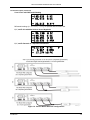
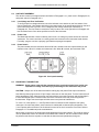
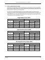
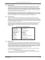
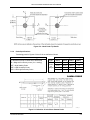
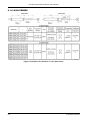
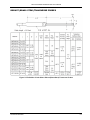
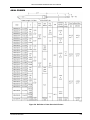
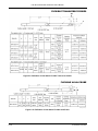
1
User’s Manual Model 460 3-Channel Gaussmeter Lake Shore Cryotronics, Inc. 575 McCorkle Blvd. Westerville, Ohio 43082-8888 USA Internet Addresses: [email protected] [email protected] Visit Our Website: www.lakeshore.com Fax: (614) 891-1392 Telephone: (614) 891-2243 Methods and apparatus disclosed and described herein have been developed solely on company funds of Lake Shore Cryotronics, Inc. No government or other contractual support or relationship whatsoever has existed which in any way affects or mitigates proprietary rights of Lake Shore Cryotronics, Inc. in these developments. Methods and apparatus disclosed herein may be subject to U.S. Patents existing or applied for. Lake Shore Cryotronics, Inc. reserves the right to add, improve, modify, or withdraw functions, design modifications, or products at any time without notice. Lake Shore shall not be liable for errors contained herein or for incidental or consequential damages in connection with furnishing, performance, or use of this material. Rev. 2.7 P/N 119-012 9 March 2015 Lake Shore Model 460 Gaussmeter User’s Manual 1. LIMITED WARRANTY STATEMENT WARRANTY PERIOD: THREE (3) YEARS Lake Shore warrants that products manufactured by Lake Shore (the "Product") will be free from defects in materials and workmanship for three years from the date of Purchaser's physical receipt of the Product (the "Warranty Period"). If Lake Shore receives notice of any such defects during the Warranty Period and the defective Product is shipped freight prepaid back to Lake Shore, Lake Shore will, at its option, either repair or replace the Product (if it is so defective) without charge for parts, service labor or associated customary return shipping cost to the Purchaser. Replacement for the Product may be by either new or equivalent in performance to new. Replacement or repaired parts, or a replaced Product, will be warranted for only the unexpired portion of the original warranty or 90 days (whichever is greater). 2. Lake Shore warrants the Product only if the Product has been sold by an authorized Lake Shore employee, sales representative, dealer or an authorized Lake Shore original equipment manufacturer (OEM). 3. The Product may contain remanufactured parts equivalent to new in performance or may have been subject to incidental use when it is originally sold to the Purchaser. 4. The Warranty Period begins on the date the Product ships from Lake Shore’s plant. 5. This limited warranty does not apply to defects in the Product resulting from (a) improper or inadequate installation (unless OT&V services are performed by Lake Shore), maintenance, repair or calibration, (b) fuses, software, power surges, lightning and non-rechargeable batteries, (c) software, interfacing, parts or other supplies not furnished by Lake Shore, (d) unauthorized modification or misuse, (e) operation outside of the published specifications, (f) improper site preparation or site maintenance (g) natural disasters such as flood, fire, wind, or earthquake, or (h) damage during shipment other than original shipment to you if shipped through a Lake Shore carrier. 6. This limited warranty does not cover: (a) regularly scheduled or ordinary and expected recalibrations of the Product; (b) accessories to the Product (such as probe tips and cables, holders, wire, grease, varnish, feed throughs, etc.); (c) consumables used in conjunction with the Product (such as probe tips and cables, probe holders, sample tails, rods and holders, ceramic putty for mounting samples, Hall sample cards, Hall sample enclosures, etc.); or, (d) non-Lake Shore branded Products that are integrated with the Product. 7. To the extent allowed by applicable law,, this limited warranty is the only warranty applicable to the Product and replaces all other warranties or conditions, express or implied, including, but not limited to, the implied warranties or conditions of merchantability and fitness for a particular purpose. Specifically, except as provided herein. Lake Shore undertakes no responsibility that the products will be fit for any particular purpose for which you may be buying the Products. Any implied warranty is limited in duration to the warranty period. No oral or written information, or advice given by the Company, its Agents or Employees, shall create a warranty or in any way increase the scope of this limited warranty. Some countries, states or provinces do not allow limitations on an implied warranty, so the above limitation or exclusion might not apply to you. This warranty gives you specific legal rights and you might also have other rights that vary from country to country, state to state or province to province. 8. Further, with regard to the United Nations Convention for International Sale of Goods (CISC,) if CISG is found to apply in relation to this agreement, which is specifically disclaimed by Lake Shore, then this limited warranty excludes warranties that: (a) the Product is fit for the purpose for which goods of the same description would ordinarily be used, (b) the Product is fit for any particular purpose expressly or impliedly made known to Lake Shore at the time of the conclusion of the contract, (c) the Product is contained or packaged in a manner usual for such goods or in a manner adequate to preserve and protect such goods where it is shipped by someone other than a carrier hired by Lake Shore. 9. Lake Shore disclaims any warranties of technological value or of non-infringement with respect to the Product and Lake Shore shall have no duty to defend, indemnify, or hold harmless you from and against any or all damages or costs incurred by you arising from the infringement of patents or trademarks or violation or copyrights by the Product. 10. THIS WARRANTY IS NOT TRANSFERRABLE. This warranty is not transferrable. 11. Except to the extent prohibited by applicable law, neither Lake Shore nor any of its subsidiaries, affiliates or suppliers will be held liable for direct, special, incidental, consequential or other damages (including lost profit, lost data, or downtime costs) arising out of the use, inability to use or result of use of the product, whether based in warranty, contract, tort or other legal theory, regardless whether or not Lake Shore has been advised of the possibility of such damages. Purchaser's use of the Product is entirely at Purchaser's risk. Some countries, states and provinces do not allow the exclusion of liability for incidental or consequential damages, so the above limitation may not apply to you. 12. This limited warranty gives you specific legal rights, and you may also have other rights that vary within or between jurisdictions where the product is purchased and/or used. Some jurisdictions do not allow limitation in certain warranties, and so the above limitations or exclusions of some warranties stated above may not apply to you. 13. Except to the extent allowed by applicable law, the terms of this limited warranty statement do not exclude, restrict or modify the mandatory statutory rights applicable to the sale of the product to you. CERTIFICATION Lake Shore certifies that this product has been inspected and tested in accordance with its published specifications and that this product met its published specifications at the time of shipment. The accuracy and calibration of this product at the time of shipment are traceable to the United States National Institute of Standards and Technology (NIST); formerly known as the National Bureau of Standards (NBS). FIRMWARE LIMITATIONS Lake Shore has worked to ensure that the Model 460 firmware is as free of errors as possible, and that the results you obtain from the instrument are accurate and reliable. However, as with any computer-based software, the possibility of errors exists. In any important research, as when using any laboratory equipment, results should be carefully examined and rechecked before final conclusions are drawn. Neither Lake Shore nor anyone else involved in the creation or production of this firmware can pay for loss of time, inconvenience, loss of use of the product, or property damage caused by this product or its failure to work, or any other incidental or consequential damages. Use of our product implies that you understand the Lake Shore license agreement and statement of limited warranty. FIRMWARE LICENSE AGREEMENT The firmware in this instrument is protected by United States copyright law and international treaty provisions. To maintain the warranty, the code contained in the firmware must not be modified. Any changes made to the code is at the user’s risk. Lake Shore will assume no responsibility for damage or errors incurred as result of any changes made to the firmware. Under the terms of this agreement you may only use the Model 460 firmware as physically installed in the instrument. Archival copies are strictly forbidden. You may not decompile, disassemble, or reverse engineer the firmware. If you suspect there are problems with the firmware, return the instrument to Lake Shore for repair under the terms of the Limited Warranty specified above. Any unauthorized duplication or use of the Model 460 firmware in whole or in part, in print, or in any other storage and retrieval system is forbidden. TRADEMARK ACKNOWLEDGMENT Many manufacturers and sellers claim designations used to distinguish their products as trademarks. Where those designations appear in this manual and Lake Shore was aware of a trademark claim, they appear with initial capital letters and the ™ or ® symbol. CalCurve™, Carbon-Glass™, Cernox™, Duo-Twist™, Gamma Probe™, Quad-Lead™, Quad-Twist™, Rox™, SoftCal™, and Thermox™ are trademarks of Lake Shore Cryotronics, Inc. MS-DOS® and Windows/95/98/NT/2000® are trademarks of Microsoft Corp. NI-488.2™ is a trademark of National Instruments. PC, XT, AT, and PS-2 are trademarks of IBM Copyright © 1993–1999, 2001, 2003-2004, 2009 and 2014-2015 by Lake Shore Cryotronics, Inc. All rights reserved. No portion of this manual may be reproduced, stored in a retrieval system, or transmitted, in any form or by any means, electronic, mechanical, photocopying, recording, or otherwise, without the express written permission of Lake Shore. Rev. 2.7 P/N 119-012 9 March 2015 Lake Shore Model 460 Gaussmeter User’s Manual Lake Shore Model 460 Gaussmeter User’s Manual Electromagnetic Compatibility (EMC) for the Model 460 3-Channel Gaussmeter Electromagnetic Compatibility (EMC) of electronic equipment is a growing concern worldwide. Emissions of and immunity to electromagnetic interference is now part of the design and manufacture of most electronics. To qualify for the CE Mark, the Model 460 meets or exceeds the generic requirements of the European EMC Directive 89/336/EEC as a CLASS A product. A CLASS A product is allowed to radiate more RF than a CLASS B product and must include the following warning: WARNING: This is a CLASS A product. In a domestic environment, this product may cause radio interference in which case the user may be required to take adequate measures. The instrument was tested under normal operating conditions with sensor and interface cables attached. If the installation and operating instructions in the User’s Manual are followed, there should be no degradation in EMC performance. Pay special attention to instrument cabling. Improperly installed cabling may defeat even the best EMC protection. For the best performance from any precision instrument, follow the grounding and shielding instructions in the User’s Manual. In addition, the installer of the Model 460 should consider the following: • • • • Leave no unused or unterminated cables attached to the instrument. Make cable runs as short and direct as possible. Do not tightly bundle cables that carry different types of signals. Add the clamp-on ferrite filter (Part Number 109-053) included with the connector kit to the serial interface cable near the instrument rear panel when that interface is used. Lake Shore Model 460 Gaussmeter User’s Manual TABLE OF CONTENTS Chapter/Paragraph Title Page 1 INTRODUCTION .................................................................................................................................................... 1-1 1.0 General .............................................................................................................................................. 1-1 1.1 Product Description ........................................................................................................................... 1-1 1.2 Specifications .................................................................................................................................... 1-4 1.3 Safety Summary ................................................................................................................................ 1-5 1.4 Safety Symbols.................................................................................................................................. 1-5 2 INSTALLATION ...................................................................................................................................................... 2-1 2.0 General .............................................................................................................................................. 2-1 2.1 Inspection and Unpacking ................................................................................................................. 2-1 2.2 Repackaging For Shipment ............................................................................................................... 2-1 2.3 Rear Panel Definition......................................................................................................................... 2-2 2.4 Line Input Assembly .......................................................................................................................... 2-3 2.4.1 Line Voltage and Fuse Verification ................................................................................................ 2-3 2.4.2 Power Cord .................................................................................................................................... 2-3 2.4.3 Power Switch ................................................................................................................................. 2-3 2.5 Probe Input Connection ..................................................................................................................... 2-3 2.5.1 Attachment To A Hall Generator .................................................................................................... 2-4 2.6 Corrected and Monitor Analog Outputs ............................................................................................. 2-4 2.7 Initial Setup and System Checkout Procedure .................................................................................. 2-4 3 OPERATION........................................................................................................................................................... 3-1 3.0 General .............................................................................................................................................. 3-1 3.1 Definition of Front Panel Controls ...................................................................................................... 3-1 3.1.1 Front Panel Keypad Definitions...................................................................................................... 3-1 3.1.2 Front Panel Display........................................................................................................................ 3-3 3.1.3 Front Panel Navigation .................................................................................................................. 3-4 3.1.4 Channel On/Off .............................................................................................................................. 3-4 3.1.5 Vector Source ................................................................................................................................ 3-5 3.2 Max Hold and Max Reset .................................................................................................................. 3-5 3.3 Zero Probe......................................................................................................................................... 3-6 3.4 Select Range and Auto Range .......................................................................................................... 3-7 3.5 AC/DC and Peak/RMS ...................................................................................................................... 3-8 3.6 Filter .................................................................................................................................................. 3-9 3.7 Field and Temperature Compensation ............................................................................................ 3-11 3.8 Gauss/Tesla .................................................................................................................................... 3-11 3.9 Relative Set and Relative On/Off ..................................................................................................... 3-12 3.10 Alarm Set and Alarm On/Off ............................................................................................................ 3-13 3.11 Local and Interface .......................................................................................................................... 3-16 3.12 Display ............................................................................................................................................. 3-17 3.13 Analog Out....................................................................................................................................... 3-17 3.13.1 Corrected Analog Out .................................................................................................................. 3-17 3.13.2 Monitor Analog Out ...................................................................................................................... 3-20 3.14 Locking and Unlocking the Keyboard .............................................................................................. 3-21 3.15 Factory Default Settings .................................................................................................................. 3-22 3.16 Special Functions ............................................................................................................................ 3-22 3.16.1 Fast Data Acquisition Mode ......................................................................................................... 3-22 3.16.2 Analog Output Control Mode........................................................................................................ 3-23 3.16.3 Sleep Mode .................................................................................................................................. 3-23 3.17 Probe Considerations ...................................................................................................................... 3-24 3.17.1 Changing Probes ......................................................................................................................... 3-24 3.17.2 Probe Handling ............................................................................................................................ 3-25 3.17.3 Probe Polarity .............................................................................................................................. 3-26 3.17.4 Probe Accuracy Considerations ................................................................................................... 3-27 4 COMPUTER INTERFACE OPERATION ................................................................................................................ 4-1 4.0 GENERAL ......................................................................................................................................... 4-1 4.1 IEEE-488 INTERFACE ...................................................................................................................... 4-1 4.1.1 Changing IEEE-488 Interface Parameters ..................................................................................... 4-2 4.1.2 IEEE-488 Command Structure....................................................................................................... 4-2 4.1.2.1 Bus Control Commands ............................................................................................................. 4-2 4.1.2.2 Common Commands ................................................................................................................. 4-3 4.1.2.3 Device Specific Commands........................................................................................................ 4-3 Table of Contents i Lake Shore Model 460 Gaussmeter User’s Manual TABLE OF CONTENTS (Continued) Chapter/Paragraph Title Page 4.1.2.4 Message Strings ......................................................................................................................... 4-3 4.1.3 Status Registers ............................................................................................................................. 4-4 4.1.3.1 Status Byte Register and Service Request Register .................................................................. 4-4 4.1.3.2 Standard Event Status Register and Standard Event Status Enable Register ........................... 4-4 4.1.4 IEEE Interface Example Programs................................................................................................. 4-5 4.1.4.1 IEEE-488 Interface Board Installation for Visual Basic Program ................................................ 4-5 4.1.4.2 Visual Basic IEEE-488 Interface Program Setup ........................................................................ 4-7 4.1.4.3 IEEE-488 Interface Board Installation for Quick Basic Program ............................................... 4-10 4.1.4.4 Quick Basic Program ................................................................................................................ 4-10 4.1.4.5 Program Operation ................................................................................................................... 4-13 4.1.5 Troubleshooting ........................................................................................................................... 4-13 4.2 Serial Interface Overview ................................................................................................................. 4-14 4.2.1 Physical Connection..................................................................................................................... 4-14 4.2.2 Hardware Support ........................................................................................................................ 4-15 4.2.3 Character Format ......................................................................................................................... 4-15 4.2.4 Message Strings .......................................................................................................................... 4-15 4.2.5 Message Flow Control ................................................................................................................. 4-16 4.2.6 Changing Baud Rate .................................................................................................................... 4-16 4.2.7 Serial Interface Basic Programs ................................................................................................... 4-17 4.2.7.1 Visual Basic Serial Interface Program Setup ............................................................................ 4-17 4.2.7.2 Quick Basic Serial Interface Program Setup............................................................................. 4-20 4.2.8 Trouble Shooting .......................................................................................................................... 4-22 4.3 Command Summary ........................................................................................................................ 4-22 4.3.1 Common Commands ................................................................................................................... 4-24 4.3.2 Interface Commands .................................................................................................................... 4-27 4.3.3 Device Specific Commands ......................................................................................................... 4-30 4.3.4 Probe Specific Commands ........................................................................................................... 4-39 5 ACCESSORIES AND PROBES ............................................................................................................................. 5-1 5.0 General .............................................................................................................................................. 5-1 5.1 Models ............................................................................................................................................... 5-1 5.2 Accessories ....................................................................................................................................... 5-1 5.3 Lake Shore Standard Probes ............................................................................................................ 5-3 5.3.1 Probe Selection Criteria ................................................................................................................. 5-3 5.3.2 Radiation Effects on Gaussmeter Probes ...................................................................................... 5-4 5.3.3 2-Axis and 3-Axis Probes ............................................................................................................... 5-4 5.3.4 Probe Specifications ...................................................................................................................... 5-5 5.4 Helmholtz Coil Low Field Standards ................................................................................................ 5-10 5.5 Reference Magnets ......................................................................................................................... 5-12 6 SERVICE ................................................................................................................................................................ 6-1 6.0 General .............................................................................................................................................. 6-1 6.1 General Maintenance Precautions..................................................................................................... 6-1 6.2 Electrostatic Discharge ...................................................................................................................... 6-1 6.2.1 Identification Of Electrostatic Discharge Sensitive Components .................................................... 6-2 6.2.2 Handling Electrostatic Discharge Sensitive Components ............................................................... 6-2 6.3 Line Voltage Selection ....................................................................................................................... 6-2 6.4 Fuse Replacement............................................................................................................................. 6-3 6.5 Rear Panel Connector Definitions...................................................................................................... 6-4 6.5.1 IEEE-488 Interface Connector ....................................................................................................... 6-5 6.6 Optional Serial Interface Cable And Adapters ................................................................................... 6-6 6.7 Operating Software Eprom Replacement .......................................................................................... 6-7 6.8 Error Messages ................................................................................................................................. 6-8 APPENDIX A – GLOSSARY OF TERMINOLOGY ....................................................................................................... A-1 APPENDIX B – UNITS FOR MAGNETIC PROPERTIES ............................................................................................. B-1 APPENDIX C – HALL GENERATORS......................................................................................................................... C-1 C1.0 General ............................................................................................................................................. C-1 C2.0 Theory of Operation .......................................................................................................................... C-1 C3.0 Hall Generator Generic Hookup ....................................................................................................... C-3 C4.0 Using a Hall Generator with the Model 460 ...................................................................................... C-4 C5.0 Specifications ................................................................................................................................... C-5 C6.0 HALLCAL.EXE Program ................................................................................................................... C-8 ii Table of Contents Lake Shore Model 460 Gaussmeter User’s Manual LIST OF ILLUSTRATIONS Figure No. 1-1 1-2 2-1 2-2 2-3 3-1 3-2 3-3 3-4 3-5 3-6 3-7 4-1 4-2 4-3 4-4 5-1 5-2 5-3 5-4 5-5 5-6 5-7 5-8 5-9 5-10 5-11 5-12 5-13 5-14 5-15 5-16 5-17 5-18 5-19 6-1 6-2 6-3 6-4 6-5 6-6 6-7 6-8 6-9 C-1 C-2 C-3 C-4 C-5 C-6 C-7 Title Page Model 460 Front Panel ................................................................................................................................. 1-1 Various Model 460 Probe Configurations ..................................................................................................... 1-3 Model 460 Rear Panel.................................................................................................................................. 2-2 Line Input Assembly ..................................................................................................................................... 2-3 Model MCBL-XX User Programmable Cable Accessory .............................................................................. 2-4 Model 460 Front Panel ................................................................................................................................. 3-1 Front Panel Display Definition ...................................................................................................................... 3-3 Display Filter Response Examples ............................................................................................................. 3-10 Monitor Analog Output Frequency Response ............................................................................................ 3-20 Maximum Flexible Probe Bend Radius ...................................................................................................... 3-25 Probe Orientation For Positive Measurement ............................................................................................ 3-26 Effect Of Angle On Measurements ............................................................................................................. 3-27 GPIB Setting Configuration .......................................................................................................................... 4-6 DEV 12 Device Template Configuration ....................................................................................................... 4-6 Typical National Instruments GPIB Configuration from IBCONF.EXE........................................................ 4-11 Serial Interface Adapters ............................................................................................................................ 4-14 2-Axis Probe Tip Details ............................................................................................................................... 5-4 3-Axis Probe Tip Details ............................................................................................................................... 5-5 Definition of Lake Shore Gamma Probe ....................................................................................................... 5-5 Definition of Lake Shore 2- and 3-Axis Probes ............................................................................................. 5-6 Definition of Lake Shore Robust (Brass Stem) Probes................................................................................. 5-6 Definition of Lake Shore Transverse Probes ................................................................................................ 5-7 Definition of Lake Shore Tangential Probe ................................................................................................... 5-7 Definition of Lake Shore Axial Probes .......................................................................................................... 5-8 Definition of Lake Shore Flexible Transverse Probes................................................................................... 5-9 Definition of Lake Shore Flexible Axial Probe .............................................................................................. 5-9 Model MH-2.5 Helmholtz Coil ..................................................................................................................... 5-10 Model MH-6 Helmholtz Coil........................................................................................................................ 5-11 Model MH-12 Helmholtz Coil...................................................................................................................... 5-11 Lake Shore Reference Magnets ................................................................................................................. 5-12 Model 4060 Zero Gauss Chamber ............................................................................................................. 5-13 Model 4065 Large Zero Gauss Chamber ................................................................................................... 5-13 Model 4001 RJ-11 Cable Assembly ........................................................................................................... 5-14 Model 4002 RJ-11 to DB-25 Adapter ......................................................................................................... 5-14 Model 4003 RJ-11 to DE-9 Adapter ........................................................................................................... 5-14 Power Fuse Access...................................................................................................................................... 6-3 PROBE INPUT Connector Details ............................................................................................................... 6-4 ANALOG OUT Corrected and Monitor BNC Connector Details ................................................................... 6-4 SERIAL I/O Connector Details ..................................................................................................................... 6-4 IEEE-488 Rear Panel Connector Details...................................................................................................... 6-5 Model 4001 RJ-11 Cable Assembly Wiring Details ...................................................................................... 6-6 Model 4002 RJ-11 to DB-25 Adapter Wiring Details .................................................................................... 6-6 Model 4003 RJ-11 to DE-9 Adapter Wiring Details ...................................................................................... 6-6 Location Of Operating Software EPROM ..................................................................................................... 6-7 Hall Generator Theory ..................................................................................................................................C-2 Axial and Transverse Configurations............................................................................................................C-2 Typical Hall Generator Hookup ....................................................................................................................C-4 Hall Generator Input Impedance ..................................................................................................................C-4 Axial Hall Generator HGA-3010, HGA-3030, & HGCA-3010 Dimensions ....................................................C-5 Transverse Hall Generator HGT-3010, HGT-3030, & HGCT-3020 Dimensions ..........................................C-5 Transverse Hall Generator HGT-1010 Dimensions ......................................................................................C-6 Table of Contents iii Lake Shore Model 460 Gaussmeter User’s Manual LIST OF TABLES Table No. 4-1 4-2 4-3 4-4 4-5 4-6 4-7 4-8 B-1 B-2 C-1 C-2 C-3 iv Title Page IEEE-488 Interface Program Control Properties ........................................................................................... 4-8 Visual Basic IEEE-488 Interface Program .................................................................................................... 4-9 Quick Basic IEEE-488 Interface Program................................................................................................... 4-12 Serial Interface Specifications .................................................................................................................... 4-15 Serial Interface Program Control Properties ............................................................................................... 4-18 Visual Basic Serial Interface Program ........................................................................................................ 4-19 Quick Basic Serial Interface Program ......................................................................................................... 4-20 Command Summary .................................................................................................................................. 4-23 Conversion from CGS to SI Units ................................................................................................................. B-1 Recommended SI Values for Physical Constants ........................................................................................ B-2 Cryogenic Hall Generator Specifications ..................................................................................................... C-5 Axial Hall Generator Specifications ............................................................................................................. C-6 Transverse Hall Generator Specifications ................................................................................................... C-7 Table of Contents Lake Shore Model 460 Gaussmeter User’s Manual CHAPTER 1 INTRODUCTION 1.0 GENERAL Lake Shore Cryotronics designed and manufactured the Model 460 3-Channel Gaussmeter in the United States of America. The Model 460 is a high-accuracy, full-featured gaussmeter ideally suited for the laboratory. Model 460 features include: • 3 Axis or 3 Independent Channels • Displays Each Axis Simultaneously • Vector Magnitude Reading • Resolution to 5¾ Digits • Accuracy to ±0.10% of Reading • Peak Capture • Analog Voltage Outputs • IEEE-488 and Serial Interface 1.1 PRODUCT DESCRIPTION The Model 460 three-channel Hall effect gaussmeter is the best choice for applications requiring three axis measurements or three simultaneous single axis measurements. This instrument combines the performance of three Model 450 Gaussmeters into one package, making it an excellent value. The large display shows readings for all three channels simultaneously. The fourth display can be used to show Vector Magnitude when necessary. Probes The Lake Shore strength in magnetic measurement instrumentation is rooted in the ability to make Hall effect sensors and probes. This strength is most apparent when multiple axis measurements are required. The Model 460 is optimized for use with Lake Shore two- and three-axis probes as well as standard Hall sensors, single axis probes, and probe accessories. The instrument automatically reads data stored in the probe connector to identify probe type and capability. If standard products are not sufficient, custom probes and assemblies are can be made to order. Measurement Features Easy access to probe information that is stored in the probe allows several features which improve the measurement capability of the instrument. Probe type tells the instrument how to configure itself for multiple axis measurements and what field ranges are available for display, autorange, and automatic probe zero. With a factory calibrated linearization table, the instrument can compensate for inherent nonlinearity in the sensor and calculate the field more accurately than a single point sensitivity would allow. If the probe is equipped with a temperature sensor, the Model 460 reads temperature along with the field signal and makes continuous adjustments to the calculated field value. Vector magnitude calculations can be done by the instrument when using two- and three-axis probes. 460_Front.bmp Figure 1-1. Model 460 Front Panel Introduction 1-1 Lake Shore Model 460 Gaussmeter User’s Manual Product Description (Continued) Measurement Modes The Model 460 has three operating modes: DC, RMS, and Peak. The instrument is well suited for DC measurements because accuracy and resolution are best in DC mode. Noise floor is so low that 5¾ digit measurements are possible. Low noise and high stability are ideal for multiple axis field mapping applications. Changing fields, which are often used in material analysis systems, can be measured on all three inputs up to 18 times a second over a computer interface with full resolution. In RMS mode the Model 460 can measure periodic AC fields from 10 to 400 Hertz. True RMS conversion is done by instrument circuitry that accommodates wave forms with crest factors up to 7. RMS mode is best suited for measuring fields surrounding linear power supplies or solenoids driven at line frequency. Peak circuitry in the Model 460 can capture single-event peaks or monitor the peak amplitude of periodic wave forms. Reproducible single-peak measurements can be made down to 5 ms. Three independent peak circuits allow simultaneous capture of all three inputs. Instrument software enables an indefinite hold time with no decay. Periodic peak measurements can be made over the same frequency range as RMS wave forms. If faster peak or RMS measurements are required, the Lake Shore Model 480 Fluxmeter has a wider frequency range. Range and Resolution Hall effect gaussmeters are popular in part because of their ability to measure field over a broad range. With appropriate probes, the Model 460 has full-scale ranges from 300 mG to 300 kG. A different range can be used with each input. With 5¾-digit resolution, DC field variations approaching 0.010 mG can be detected. In larger DC fields, resolution of 1 part in 300,000 can be achieved. RMS and peak measurements are limited to 4¾ digits or 1 part in 30,000 resolution because environmental noise is more difficult to separate from desired signal in those modes. The filter feature can be used to improve resolution in noisy environments by taking a running average of field readings in DC or RMS modes. Interface There are two computer interfaces included with the Model 460: parallel IEEE-488 and serial RS-232C. Either interface can send instrument setup commands and query field reading data. The maximum reading rate of the instrument can be achieved using the IEEE-488 interface. Nearly every function of the instrument front panel can be performed over the computer interface. Two types of analog voltage outputs are also included with the Model 460. The single Corrected Analog Output is a DC voltage proportional to the display reading. It is generated using a D/A converter programmed at the instrument update rate. Available software error correction and vector calculations can be used when generating the corrected output voltage. Three Monitor outputs are real-time analog voltages proportional to the field at each input. These outputs do not have the advantage of software correction but are much faster than the Corrected output with the full DC to 400 Hertz bandwidth. Operation The Model 460 has several software features intended to make multi-axis field measurements more convenient. A bright four line vacuum fluorescent display and full function keypad provide easy access to these features and give meaningful feedback. X, Y, and Z Axis with Vector Magnitude + 46.003 G DC + 100.0 12 G DC +200.00 1 G DC +228.292 G XYZ The Model 460 can display each axis simultaneously plus Vector Magnitude XYZ = (X 2 + Y2 + Z2)1/2. 1-2 Introduction Lake Shore Model 460 Gaussmeter User’s Manual Product Description (Continued) X and Y Axis with Differential Reading + 105.628 + 83.4 15 G DC G DC + 22.2 13 G X-Y Differential readings (X – Z = Xreading – Yreading) are possible with the Model 460. X, Y, and Z Axis with Max Hold on Vector Magnitude + 58. 190 + 109.752 + 198.25 1 +2 15.936 G G G G DC DC DC MAX X, Y, and Z Channels as 3 Separate Gaussmeters +2 13.524 G DC + 5.067 G RMS + 17.374 kG PK ª C-460-1-2.eps Figure 1-2. Various Model 460 Probe Configurations Introduction 1-3 Lake Shore Model 460 Gaussmeter User’s Manual 1.2 SPECIFICATIONS General Measurement Number of Inputs: 3 Update Rate: up to 4 readings per second on display; up to 14 readings per second with IEEE-488 interface Measurement Modes: DC, RMS, Peak Probe Compatibility: Standard, multi-axis, and custom probes Probe Features: Linearity Correction, Temperature Correction, Auto Probe Zero, Differential Reading, Vector Magnitude Measurement Features: Auto Range, Max Hold, Relative Mode, Filter Probe Connector: 15 pin D style DC Measurement DC Display Resolution: 5¾ digits with filter, 4¾ digits without filter Range HST Probe 300 kG 30 kG 3 kG 300 G HSE Probe 30 kG 3 kG 300 G 30 G UHS Probe 30 G 3G 300 mG Resolution w/ Filter Resolution w/out Filter 0.001 kG 0.0001 kG 0.00001 kG 0.001 G 0.01 kG 0.001 kG 0.0001 kG 0.01 G 0.0001 kG 0.00001 kG 0.001 G 0.0001 G 0.001 kG 0.0001 kG 0.01 G 0.001 G 0.0001 G 0.00001 G 0.001 mG 0.001 G 0.0001 G 0.01 mG DC Accuracy: ±0.10% of reading ±0.005% of range DC Temperature Coefficient: ±0.05% of reading ±0.03% of range/°C AC RMS & Peak Measurement AC Display Resolution: 4¾ digits Range HST Probe 300 kG 30 kG 3 kG 300 G HSE Probe 30 kG 3 kG 300 G 30 G UHS Probe 30 G 3G 300 mG RMS Resolution Peak Resolution 0.01 kG 0.001 kG 0.0001 kG 0.01 G 0.01 kG 0.001 kG 0.0001 kG — 0.001 kG 0.0001 kG 0.01 G 0.001 G 0.001 kG 0.0001 kG 0.01 G — 0.001 G 0.0001 G 0.01 mG 0.001 G 0.0001 G — AC Frequency Range: 10 – 400 Hz AC RMS Accuracy: ±2% of reading (50 – 60 Hz) AC RMS Freq. Response: 0 to -3.5% of reading (10 – 400 Hz) (All AC RMS specifications for sinusoidal input >1% of range) AC Peak Accuracy: ±5% typical AC Peak Speed: 5 ms for single peak Front Panel Display Type: 4 line by 20 character, vacuum fluorescent Display Resolution: Up to ±5¾ digits Display Update Rate: 4 rdgs/sec. Vector Off, 3 rdgs/sec On Displays Units: Gauss (G), Tesla (T) Units Multipliers: µ, m, k Annunciators: RMS AC input signal DC DC input signal MAX Max Hold value ° Relative reading R Remote operation ª Alarm on 1-4 Keypad: 25 full travel keys Front Panel Features: Intuitive operation, display prompts, front panel lockout, brightness control Interfaces RS-232C Capabilities: Baud: 300, 1200, 9600 Connector: RJ-11 configuration Update Rate: Up to 14 readings per second IEEE-488 Capabilities: Complies with IEEE-488.2: SH1 AH1 SR1 RL1 PP0 DC1 DT0 C0 E1 Software Support: LabView Driver Update Rate: 18 rdgs/sec. Vector Off, 14 rdgs/sec. Vector On Alarm: Settings: High and low set point, Inside/Outside, Audible Actuators: Display annunciator, beeper Monitor Analog Output (3) Configuration: Real-time analog voltage output Scale: ±3 V = ±FS on selected range Frequency Response: DC to 400 Hz Accuracy: Probe dependent Minimum Load Resistance: 1 k (short circuit protected) Connector: BNC Corrected Analog Output (1) Configuration: Voltage output generated by DAC Range: ±3 V; ±10 V for Model 460-10 Scale: User defined Resolution: 0.366 mV of ±3 V Update Rate: Same as field measurement Accuracy: ±0.1% of full scale in addition to measurement error Minimum Load Resistance: 1 k (short circuit protected) Connector: BNC General Ambient Temperature: 15 – 35 °C at rated accuracy. 5 – 40 °C with reduced accuracy Power Requirement: 100, 120, 220, 240 VAC (+5%, -10%), 50 or 60 Hz, 40 watts Size: 434 W x 89 H x 369 mm D (17.1 x 3.5 x 14.5 in.), half rack Weight: 7.5 kilograms (16.5 pounds) Approval: CE Mark Ordering Information Part number Description Instrument 460 Model 460 Gaussmeter, ±3 V corrected analog output 460-10 Model 460 Gaussmeter, ±10 V corrected analog output Accessories Included 115-006 Detachable line cord (U.S.) 115-007 Detachable line cord (European) 4060 Zero gauss chamber MAN-460 Model 460 Gaussmeter User's Manual Accessories Available 4001 RJ-11 cable assembly 4002 RJ-11 to DB-25 adapter 4003 RJ-11 to DE-9 adapter 4004 IEEE-488 cable, 1 meter (3 feet) 4065 Large zero gauss chamber for Gamma probe RM-1 Rack mount kit for one 460 gaussmeter MCBL-6 User programmable cable with PROM (6' long) MCBL-20 User programmable cable with PROM (20' long) MPEC-10 Probe extension cable with EEPROM (10' long) MPEC-25 Probe extension cable with EEPROM (25' long) MPEC-50 Probe extension cable with EEPROM (50' long) MPEC-100 Probe extension cable with EEPROM (100' long) (Extension cables must be matched to probes) Probes Ordered Separately Custom Probes Available (Consult Lake Shore for more information) Specifications are subject to change without notice. Introduction Lake Shore Model 460 Gaussmeter User’s Manual 1.3 SAFETY SUMMARY Observe these general safety precautions during all phases of instrument operation, service, and repair. Failure to comply with these precautions or with specific warnings elsewhere in this manual violates safety standards of design, manufacture, and intended instrument use. Lake Shore Cryotronics, Inc. assumes no liability for Customer failure to comply with these requirements. The Model 460 protects the operator and surrounding area from electric shock or burn, mechanical hazards, excessive temperature, and spread of fire from the instrument. Environmental conditions outside of the conditions below may pose a hazard to the operator and surrounding area. • Temperature: 5 C° to 40 °C. • Maximum relative humidity: 80% for temperature up to 31 °C decreasing linearly to 50% at 40 °C. • Power supply voltage fluctuations not to exceed ±10% of the nominal voltage. Ground The Instrument To minimize shock hazard, connect the instrument chassis and cabinet to an electrical ground. The instrument is equipped with a three-conductor AC power cable. Plug the power cable into an approved three-contact electrical outlet or use a three-contact adapter with the grounding wire (green) firmly connected to an electrical ground (safety ground) at the power outlet. The power jack and mating plug of the power cable meet Underwriters Laboratories (UL) and International Electrotechnical Commission (IEC) safety standards. Do Not Operate In An Explosive Atmosphere Do not operate the instrument or probes in the presence of flammable gases or fumes. Operation of any electrical instrument in such an environment constitutes a definite safety hazard. Keep Away From Live Circuits Operating personnel must not remove instrument covers. Refer component replacement and internal adjustments to qualified maintenance personnel. Do not replace components with power cable connected. To avoid injuries, always disconnect power and discharge circuits before touching them. Do Not Substitute Parts Or Modify Instrument Do not install substitute parts or perform any unauthorized modification to the instrument. Return the instrument to an authorized Lake Shore Cryotronics, Inc. representative for service and repair to ensure that safety features are maintained. 1.4 SAFETY SYMBOLS Introduction 1-5 Lake Shore Model 460 Gaussmeter User’s Manual This Page Intentionally Left Blank 1-6 Introduction Lake Shore Model 460 Gaussmeter User’s Manual CHAPTER 2 INSTALLATION 2.0 GENERAL This chapter provides general Model 460 installation instructions: inspection and unpacking in Paragraph 2.1, repackaging for shipment in Paragraph 2.2, definition of rear panel connections in Paragraph 2.3, and initial setup and system checkout procedure in Paragraph 2.4. 2.1 INSPECTION AND UNPACKING Inspect shipping containers for external damage. Make all claims for damage (apparent or concealed) or partial loss of shipment in writing to Lake Shore within five (5) days from receipt of goods. If damage or loss is apparent, please notify the shipping agent immediately. Open the shipping containers. Use the packing list included with the system to verify receipt of the instrument, probes, accessories, and manual. Inspect for damage. Inventory all components supplied before discarding any shipping materials. If there is freight damage to the instrument, file proper claims promptly with the carrier and insurance company and notify Lake Shore. Notify Lake Shore immediately of any missing parts. Lake Shore cannot be responsible for any missing parts unless notified within 60 days of shipment. Refer to the standard Lake Shore Warranty on the A Page (behind the title page). 2.2 REPACKAGING FOR SHIPMENT If it is necessary to return the Model 460, probe(s), or accessories for repair or replacement, a Return Goods Authorization (RGA) number must be obtained from a factory representative before returning the instrument to our service department. When returning an instrument for service, the following information must be provided before Lake Shore can attempt any repair. 1. Instrument model and serial number. 2. User’s name, company, address, and phone number. 3. Malfunction symptoms. 4. Description of system. 5. Returned Goods Authorization (RGA) number. If possible, the original packing material should be retained for reshipment. If not available, consult Lake Shore for shipping and packing instructions. Because of their fragility, Lake Shore probes are shipped in special cardboard and foam boxes. These boxes should be retained for storage of probes while the gaussmeter is not in use. The same box can be used to return probes to Lake Shore for recalibration or repair. Installation 2-1 Lake Shore Model 460 Gaussmeter User’s Manual 2.3 REAR PANEL DEFINITION This paragraph provides a description of the Model 460 rear panel connections. The rear panel consists of the line input assembly, IEEE-488 Interface Connector, Serial I/O Connector, Probe Input Connectors, and Corrected and Monitor Analog Output BNCs. This paragraph is provided for information only. Please read the entire paragraph then proceed to Paragraph 2.7 for the initial setup and system checkout procedure. Rear panel connector pin-out details are provided in Chapter 6 – Service. CAUTION: Verify AC Line Voltage shown in the fuse holder window is appropriate for the intended AC power input. Also remove and verify the proper fuse is installed before plugging in and turning on the instrument. CAUTION: Always turn off the instrument before making any rear panel connections. This is especially critical when making probe to instrument connections. 460_Back.bmp Description Pin Definition Paragraph 2.4 Figure 2-2 IEEE-488 INTERFACE Connector Paragraph 6.5.1 Figure 6-5 SERIAL I/O RJ-11 Connector Paragraph 4.2.1 Figure 6-4 ANALOG OUT Corrected BNC Paragraph 2.6 and 3.13.1 Figure 6-3 ANALOG OUT Monitor BNC (Quantity 3) Paragraph 2.6 and 3.13.2 Figure 6-3 Paragraph 2.5 Figure 6-2 Line Input Assembly PROBE INPUT 15 pin D-Style Connector (Quantity 3) Figure 2-1. Model 460 Rear Panel 2-2 Installation Lake Shore Model 460 Gaussmeter User’s Manual 2.4 LINE INPUT ASSEMBLY This section covers line voltage and fuse verification in Paragraph 2.4.1, power cord in Paragraph 2.4.2, and power switch in Paragraph 2.4.3. 2.4.1 Line Voltage and Fuse Verification To verify proper line voltage selection look at the indicator in the window on the fuse drawer of the line input assembly. Line voltage should be in the range shown in the specifications listed on the back of the instrument. See Figure 2-2. If not, change the line voltage selector per instructions in Paragraph 6.3. The fuse must be removed to verify its value, refer to the procedure in Paragraph 6.4. Use slow-blow fuses of the value specified on back of the instrument. 2.4.2 Power Cord The Model 460 includes a three-conductor power cord. Line voltage is present across the outer two conductors. The center conductor is a safety ground and connects to the instrument metal chassis. For safety, plug the cord into a properly grounded three-pronged receptacle. 2.4.3 Power Switch The power switch turns the instrument On and Off and is located in the line input assembly on the instrument rear. When l is raised, the instrument is On. When O is raised, the instrument is Off. F-460-2-2.eps Figure 2-2. Line Input Assembly 2.5 PROBE INPUT CONNECTION WARNING: Some probes used with the gaussmeter have conductive parts. Never probe near exposed live voltage. Personal injury and damage to the instrument may result. CAUTION: Always turn off the instrument before making any rear panel Probe Input connections. Lake Shore probes plug into three 15 pin D-style connectors on the rear panel. Turn the instrument off before attaching a probe. Align the probe connector with the rear panel connector and push straight in to avoid bending the pins. For best results, secure the connector to the rear panel using the two thumbscrews. A tight connector keeps the cable secure and prevents interference. To use a 2 or 3-Axis probe, X, Y, and Z probes must be connected to their respective rear panel connectors. On multi-axis probes, each connector is marked with a channel (axis) designation. The Y and Z probes will not function if the X channel is turned off or the X connector is removed. Refer to Paragraph 3.17 for additional probe considerations. When power is turned on, the instrument reads parameters from probe memory. The probe is ready to use. No parameters need to be entered into the Model 460. However, the Zero Probe function should be performed the first time a probe is used with the instrument and periodically during use. Installation 2-3 Lake Shore Model 460 Gaussmeter User’s Manual 2.5.1 Attachment To A Hall Generator The Model MCBL-XX has a 15 pin D-Style connector on one end for direct attachment to any of the PROBE INPUT connections on the back panel of the Model 460 Gaussmeter. Four tinned wires are provided for connection to the Hall Generator. The leads may be soldered directly to these wires. The cable comes in two lengths: the MCBL-6 is 2 meters (6 feet) and the MCBL-20 is 6 meters (20 feet). F-460-2-3.eps Figure 2-3. Model MCBL-XX User Programmable Cable Accessory CAUTION: The Hall Generator should be isolated from all line voltages (or voltages referenced to earth ground). If not, damage to the Model 460 Gaussmeter is almost a certainty. Refer to Appendix C for a complete list of compatible Hall generators manufactured by Lake Shore. Once connections are made, refer to Paragraph C6.0 for instructions on using the Hallcall.exe program to store probe parameters in the internal EPROM. 2.6 CORRECTED AND MONITOR ANALOG OUTPUTS Analog outputs are available on Bayonet Nut Connectors (BNCs). The signal is on the center conductor while the outer casing is for ground. All outputs may be used simultaneously. The corrected output is not a real-time signal, but is updated at the same rate as the display. The monitor outputs are live analog signals proportional to the magnetic flux density waveform of the respective channel. Refer to Paragraph 3.13 for further operational information. 2.7 INITIAL SETUP AND SYSTEM CHECKOUT PROCEDURE This procedure verifies basic unit operation before initial use for measurements. CAUTION: Check power source for proper voltage before connecting line cord to the Model 460. Check power setting on fuse drawer window. Damage may occur if connected to improper voltage. 1. Check power source for proper voltage. The Model 460 operates with 100, 120, 220, or 240 (+5%, –10%) AC input voltage. If incorrect, refer to Paragraph 6.3. 2. Check fuse drawer window for proper voltage setting. If incorrect, refer to Paragraph 6.4. 3. Ensure power switch is off (O). CAUTION: The probe must be connected to the rear of the unit before applying power to the gaussmeter. Damage to the probe may occur if connected with power on. 4. Plug in the DA-15 probe connector to PROBE INPUT. Use thumbscrews to tighten connector to unit. 5. Connect and check all other rear panel connections (ANALOG OUTPUTS and IEEE-488 or SERIAL I/O) before applying power to the unit. 6. Plug line cord into receptacle. 2-4 Installation Lake Shore Model 460 Gaussmeter User’s Manual Initial Setup And System Checkout Procedure (Continued) 7. Turn power switch on (I). The front panel display turns on and briefly displays the following message. Lake Shore 460 Field Monitor 8. The normal gaussmeter display appears (similar to below). + + + 0.02 0.0 1 0.00 0.02 kG kG kG kG DC DC DC XYZ NOTE: For best results, the instrument and probe should warm up for at least 5 minutes before zeroing the probe, and at least 30 minutes for rated accuracy. The probe and the zero gauss chamber should be at the same temperature. NOTE: Some Lake Shore probes come with a clear plastic sleeve to protect the probe tip when not in use. The sleeve slides up and down the probe cable. To place the probe in the zero gauss chamber, slide the protective sleeve back, exposing the probe tip, before placing the tip in the chamber. 9. Place the probe in the zero gauss chamber. Once inserted, press the Channel key (in this case, Channel X), then press the Zero Probe key. You will see the following display. Press Enter With Probe At Zero Setting Channel X 10. Press the Enter key. The *CALIBRATING* message briefly displays, followed by the normal display. Do not move the probe while the *CALIBRATING* message displays. There should be a near-zero reading on the display when finished. 11. Repeat Steps 9 and 10 for the Y and Z probes, if present. NOTE: If the unit has performed well to this point, the unit is functioning properly. If you have a reference magnet available, you can continue with the test using the magnet to verify the accuracy of the Model 460. Installation 2-5 Lake Shore Model 460 Gaussmeter User’s Manual Initial Setup And System Checkout Procedure (Continued) 12. If continuing the procedure with a reference magnet, ensure the probe can accommodate the range of the magnet. Use the Range key to select the proper range. Set the display for DC. Finally, since orientation of the probe is very selective, press the Max Hold key. This will capture the highest reading (normally the reference magnet calibration value). CAUTION: Care must be exercised when handling the probe. The tip of the probe is very fragile. Any excess force may break the probe. NOTE: Probe readings are dependent upon the angle of the tip in relation to the magnetic field. (This does not apply to 3-axis probes.) This and other effects on probe operation are explained in Paragraph 3.17. 13. Carefully place probe into reference magnet. You may have to hunt around for the maximum reading. For this example, we are using a 999 ±1% Gauss Reference Magnet. Our reading appeared as follows: +0.9950 kG MAX Assuming we are using a probe attached to the X axis, the maximum reading captured was 0.9950 kG, which is within the tolerance of the reference magnet. The reading will change as the probe moves around, but will eventually remain fixed on the highest reading. To recapture a new maximum value, press the Max Reset key. 14. Repeat Steps 12 and 13 for the Y and Z probes, if present. 15. Once this abbreviated checkout procedure is successfully completed, the unit is ready for normal operation. Please proceed to Chapter 3 for further operational information. 2-6 Installation Lake Shore Model 460 Gaussmeter User’s Manual CHAPTER 3 OPERATION 3.0 GENERAL This chapter describes Model 460 3-Channel Gaussmeter operation. The front panel controls are described in Paragraph 3.1. Paragraphs 3.2 thru 3.14 describe the various front panel functions in detail. Model 460 default settings are defined in Paragraph 3.15. Special functions available over computer interface are discussed in Paragraph 3.16. Finally, probe considerations are presented in Paragraph 3.17. Refer to Chapter 4 for information on remote operation (via IEEE-488/Serial). 3.1 DEFINITION OF FRONT PANEL CONTROLS This paragraph provides a description of the front panel controls on the Model 460. The front panel consists of two major sections: a description of the 25 front panel keys in Paragraph 3.1.1, and a description of the front panel display in Paragraph 3.1.2. Front panel navigation is described in Paragraph 3.1.3. Turning channels on and off is described in Paragraph 3.1.5. Finally, the various Vector Magnitude settings are described in Paragraph 3.1.5. 3.1.1 Front Panel Keypad Definitions The keys on the front panel are defined as follows. Note the following are abbreviated descriptions of each key. A more detailed description of each function is provided in subsequent paragraphs. X Selects Channel X. Once pressed, selection of any subsequent channel specific functions (relative, alarm, range, etc.) will affect Channel X. Press and hold to turn the channel off. Refer to Paragraph 3.1.3. Y Selects Channel Y. Once pressed, selection of any subsequent channel specific functions will affect Channel Y. Press and hold to turn the channel off. Refer to Paragraph 3.1.3. Z Selects Channel Z. Once pressed, selection of any subsequent channel specific functions will affect Channel Z. Press and hold to turn the channel off. Refer to Paragraph 3.1.3. Vector Magnitude Selects Vector Magnitude. Once pressed, selection of any subsequent specific functions will affect the Vector Magnitude. Press and hold to set the vector source. Refer to Paragraphs 3.1.3 and 3.1.4. Max Reset Works with the Max Hold function. Clears Max reading back to normal field reading. Refer to Paragraph 3.2. Max Hold Turns Max Hold feature on or off. Max Hold captures and displays the highest field reading. Use Max Reset key to clear reading. Refer to Paragraph 3.2. 460_Front.bmp Figure 3-1. Model 460 Front Panel Operation 3-1 Lake Shore Model 460 Gaussmeter User’s Manual Front Panel Keypad Definitions (Continued) Zero Probe Used to zero or null effects of ambient low level fields from the probe. This function is not available for Vector Magnitude. Refer to Paragraph 3.3. Select Range Push to manually select the field measurement range. Available ranges are dependent on which probe is installed. This function is not available for Vector Magnitude. Refer to Paragraph 3.4. Auto Range Turns the Auto Range feature on and off. Allows the Model 460 to automatically select the field measurement range. This function is not available for Vector Magnitude. Refer to Paragraph 3.4. AC/DC Selects periodic (AC) or static (DC) magnetic fields. The AC selection provides the user with the choice of Peak or RMS readings. This function is not available for Vector Magnitude. Refer to Paragraph 3.5. Peak/RMS The AC selection provides the user with the choice of Peak or Root Mean Square (RMS) readings. AC peak can also be used with the Max Hold feature to measure single pulse peak values. This function is not available for Vector Magnitude. Refer to Paragraph 3.5. Filter Turns the filter on or off and allows configuration of filter. Filter on enables high resolution DC readings. Press and hold Filter key to select Field Compensation and Temperature Compensation on or off. This function is not available for Vector Magnitude. Refer to Paragraph 3.6. Gauss/Tesla Changes display units from gauss to tesla. Gauss (G) is used in the cgs system, where 1 G = 10–4 T. Tesla (T) is used in the SI system, where 1 T = 104 G. This is a global setting (applies to all channels). Refer to Paragraph 3.8. Relative Set With the relative feature turned on, this key is used to capture the present field reading as the relative setpoint. You also have the option of entering a number via the numerical keypad. Works with the Relative On/Off key. Refer to Paragraph 3.9. Relative On/Off Turns on the relative feature which displays the positive or negative deviation from the relative setpoint. The relative feature can also be used with the Max Hold and Alarm features. Refer to Paragraph 3.9. 3-2 Alarm Set This key is used to set the high and low alarm points. The alarm setpoints are absolute (unsigned) i.e., the positive or negative aspect of the field reading is ignored. Refer to Paragraph 3.10. Alarm On/Off Turns the alarm feature on or off. Press and hold the Alarm On/Off key to turn the audible alarm on or off and select the alarm to activate inside or outside the range. Refer to Paragraph 3.10. Local This key is used to select local or remote operation. When set to Local, the unit responds to front panel controls. When set to Remote, the unit is controlled via the IEEE-488 Interface. Refer to Paragraph 3.11. Interface Sets the bus address and terminators for the IEEE-488 Interface and Baud rate for the Serial Interface. Refer to Paragraph 3.11. Display Use this key to set the display brightness. Refer to Paragraph 3.12. Analog Out Used to set the source and scaling of the Corrected Analog Output. The scaling of the three Monitor Analog Outputs cannot be modified. Refer to Paragraph 3.13. Operation Lake Shore Model 460 Gaussmeter User’s Manual Front Panel Keypad Definitions (Continued) 3.1.2 Escape Terminates a function without making changes to the existing settings. Press and hold the Escape key for 20 seconds to reset the instrument and return parameters to factory default values. Refer to Paragraph 3.15. s The up triangle (s) serves two functions. The first is to toggle between various settings shown in the display. The second is to increment a numerical display. t The down triangle (t) serves two functions. The first is to toggle between various settings shown in the display. The second is to decrement a numerical display. Enter The Enter key is used to accept changes made in the field display. Press and hold the Enter key to gain access to the Keypad Lock display. A 3-digit code may be entered to lockout the keypad from accepting changes. Refer to Paragraph 3.14. Front Panel Display In normal operation, the four row by twenty character vacuum fluorescent display provides readings for Channel X on the first line, Channel Y on the second line, Channel Z on the third line, and Vector Magnitude (if selected) on the fourth line of the display. Other information is displayed when using the various functions on the keypad. Each character is comprised of a 5 by 7 dot matrix. Note the extra digit on the display will only appear if the channel is in DC mode and the Filter is turned on. See Figure 3-2. C-460-3-2.eps Figure 3-2. Front Panel Display Definition Operation 3-3 Lake Shore Model 460 Gaussmeter User’s Manual 3.1.3 Front Panel Navigation Information in the first line of the display pertains to Channel X, the second line to Channel Y, third line to Channel Z, and the fourth line to the Vector Magnitude. To select a function for a channel, you must first push the X, Y, Z, or Vector Magnitude key. Once selected, all subsequent channel specific operations will affect that channel until another channel key is pressed. The following is an example of how channel selection works. If you want to turn Max Hold on for Channel X, you must first press the Channel X key. You will briefly see the following display. Setting Channel X -0.26776 kG DC -0.90952 kG DC -0.95325 kG XYZ You may then press the Max Hold key. You will see the following display. (The Max Hold function is described in detail in Paragraph 3.2). Max Hold -0.26776 -0.90952 +0.95325 ON kG DC kG DC kG XYZ In fact, you may press any number of applicable functions and they all will affect Channel X. This will continue until another channel or the Vector Magnitude key is pressed, or the unit is turned off (in which case, it will default back to Channel X). After a short timeout, the X channel display will return to normal, with the Max Hold value being displayed on the first line as seen in the following display. -0.09228 -0.26776 -0.90952 +0.95260 3.1.4 kG kG kG kG MAX DC DC DC Channel On/Off Each channel may be independently turned on or off. To do this, press and hold the X, Y, Z, or Vector Magnitude key. For example, if we wanted to turn Channel X on, we would press and hold the Channel X key. You will see the following display. Select With °® Channel ¡On Off Setting Channel X Use the s or t arrow keys to toggle the channel on or off. Press the Enter key to select a new setting, or press the Escape key (or wait for the time out) to exit and retain the old setting. If the channel is turned off, the line in the display will be blank (and the excitation current will be turned off to the X, Y, or Z channels). Do no turn off the X-channel when using a multi-axis probe. If no probe is attached to a channel, the corresponding display will be blank (regardless if the channel is turned on or off). 3-4 Operation Lake Shore Model 460 Gaussmeter User’s Manual 3.1.5 Vector Source In addition to turning the Vector Magnitude display on or off, the source of the Vector display must also be selected. Press and hold the Vector Magnitude key until the display reads Channel ON, then press the Enter key. You will see the following display. Select With °® Vector Source XYZ Use the s or t arrow keys to toggle the vector source between XYZ, XY, XZ, YZ, and X–Y. Press the Enter key to select a new setting, or press the Escape key (or wait for the timeout) to exit and retain the old setting. The vector source will be shown in the normal display. However, if Max Hold is selected for the vector magnitude display, the identifier MAX will appear in the normal display instead of the vector source. The following is a mathematical description of the components that comprise the Vector Magnitude source. (Full 3-axis) (In the X-Y plane) (In the X-Z plane) (In the Y-Z plane) (Differential) 3.2 MAX HOLD AND MAX RESET The Max Hold function displays the largest field magnitude measured since the last Max Reset. When the Max Hold key is pressed, the currently selected channel will change to display the MAX reading. For example, to turn Max Hold on for Channel Y, press the Channel Y key, followed by the Max Hold key. You will see the following display. -0.09228 Max Hold -0.90952 +0.95325 kG DC ON kG DC kG XYZ After a short timeout, the Y channel display will return to normal, with the Max hold value being displayed on the second line of the display as seen in the following display. -0.09228 -0.26776 -0.90952 +0.95325 Operation kG kG kG kG DC MAX DC XYZ 3-5 Lake Shore Model 460 Gaussmeter User’s Manual Max Hold and Max Reset (Continued) The Max Reset key clears the Max Hold value. The Max Hold value is also reset upon power up or when changing from AC or DC. Max Hold may also be used in conjunction with the Relative display (refer to Paragraph 3.9). Max Hold functions differently when being used with AC or DC fields as follows. In DC operation, the Max Hold feature holds the field reading that is largest in magnitude. This is intended to monitor slowly changing signals. A field change not visible on the display can not be recorded in DC Max Hold. The display shows only the magnitude of the maximum reading. In AC RMS operation, the maximum RMS value displayed is held, i.e., operates the same as DC Max. In AC Peak operation, a hardware circuit traps peaks in the Hall voltage. In this mode, the unit displays the magnitude of the highest peak of an impulse or event. For best accuracy, the event must be at full amplitude for at least a few milliseconds. In the case of the Vector Magnitude display, turning on Max Hold will cause the vector source display to be replaced with MAX. Turning on Max Hold for Vector Magnitude means the maximum value calculated will be displayed. It does not mean each of the individual component max hold readings are used to form the Vector Magnitude display. When Max Hold for the Vector Magnitude is turned off, but Max Hold for the X, Y, or Z channels is on, the individual maximums are for display only and are not used for the calculation of the Vector Magnitude display. 3.3 ZERO PROBE The zero probe function is used to null (cancel) out the zero offset of the probe or small magnetic fields. It is normally used in conjunction with the zero gauss chamber, but may also be used with an unshielded probe (registering the local earth magnetic field). If three separate probes are being used, each probe may be independently zeroed. For the three-axis probes, each axis may be independently zeroed. Users wishing to cancel large magnetic fields must use the Relative function. The zero probe function is not available for the Vector Magnitude display. NOTE: For best results, the instrument and probe should warm up for at least 5 minutes before zeroing the probe, and at least 30 minutes for rated accuracy. The probe and the zero gauss chamber should be at the same temperature. NOTE: Some Lake Shore probes are equipped with a clear plastic sleeve intended to protect the tip of the probe when not being used. The sleeve is designed to slide up and down the probe cable. If you need to place the probe in the zero gauss chamber, you must slide the protective sleeve back, exposing the tip of the probe, before placing the tip in the chamber. To zero the probe in the zero gauss chamber, first allow the temperature of the probe and chamber to equalize. (A large temperature discrepancy affects the quality of the calibration.) Carefully place the probe tip into the chamber. Orientation of the probe is not critical. Once inserted, press the channel key (in this case, Channel X), then press the Zero Probe key and observe the following display. Press Enter With Probe At Zero Setting Channel X Press the Enter key. The *CALIBRATING* message is displayed, followed by a return to the normal display. Do not move the probe while calibrating. The probe is now zeroed. For best results, periodic zeroing of the probe is recommended. 3-6 Operation Lake Shore Model 460 Gaussmeter User’s Manual 3.4 SELECT RANGE AND AUTO RANGE Each channel of the Model 460 is capable of reading any of the Lake Shore probe types: High Stability, High Sensitivity, or Ultra-High Sensitivity. The three probes permit the Model 460 to sense fields as low as 0.01 mG and as high as 300 kG. The full scale ranges for each probe sensitivity, along with the fixed display resolution, are shown in the following tables. The range for the Vector Magnitude display is not directly settable. Instead, Vector Magnitude will display the same resolution as the highest range setting of the component channels. For example, if the Vector Magnitude is set for XYZ, and all three channels are in the ±3 kG range, the Vector Magnitude range will also be ±3 kG. If one of the channels is switched to ±30 kG (does not matter which one), the Vector Magnitude range will also switch to ±30 kG. High Stability Probe (HST) Range ±300 kG Gauss Resolution AC, or DC DC Filter On with Filter Off ±0.01 kG ±0.001 kG Range ±30 T Tesla Resolution AC, or DC DC Filter On with Filter Off ±0.001 T ±0.0001 T ±30 kG ±0.001 kG ±0.0001 kG ±3 T ±0.0001 T ±0.00001 T ±3 kG ±0.0001 kG ±0.00001 kG ±300 mT ±0.01 mT ±0.001 mT ±300 G ±0.01 G ±0.001 G ±30 mT ±0.001 mT ±0.0001 mT High Sensitivity Probe (HSE) Range ±30 kG Gauss Resolution AC, or DC DC Filter On with Filter Off ±0.001 kG ±0.0001 kG Range ±3 T Tesla Resolution AC, or DC DC Filter On with Filter Off ±0.0001 T ±0.00001 T ±3 kG ±0.0001 kG ±0.00001 kG ±300 mT ±0.01 mT ±0.001 mT ±300 G ±0.01 G ±0.001 G ±30 mT ±0.001 mT ±0.0001 mT ±30 G ±0.001 G ±0.0001 G ±3 mT ±0.0001 mT ±0.00001 mT Ultra-High Sensitivity Probe (UHS) Range ±30 G Operation Gauss Resolution AC, or DC DC Filter On with Filter Off ±0.001 G ±0.0001 G Range ±3 mT Tesla Resolution AC, or DC DC Filter On with Filter Off ±0.0001 mT ±0.00001 mT ±3 G ±0.0001 G ±0.00001 G ±300 µT ±0.01 µT ±0.001 µT ±300 mG ±0.01 mG ±0.001 mG ±30 µT ±0.001 µT ±0.0001 µT 3-7 Lake Shore Model 460 Gaussmeter User’s Manual Select Range and Auto Range (Continued) For manual ranging, first press the desired channel, in this case, press the channel X key. Then press the Select Range key. This allows the user to see the full scale value for the present range as follows. Select With °® +/-300.00 kG Range Setting Channel X Press the Select Range or s or t keys to cycle through the allowable full scale ranges for the probe installed. Use the Enter key to accept the new range or Escape key to retain the old range. Changing ranges in this way disables the Auto Range function until Auto Range is turned on. NOTE: When operating in AC Peak Mode only, you cannot select the lowest range for the probe installed. This is true for both Manual and Auto Range. NOTE: If a range is manually selected that is too small for the reading, the reading will disappear and the letters “OL” (for over load) will be displayed. If displaying the Vector reading, any channel displaying OL will also cause the Vector display to display OL. In Auto Range mode, the Model 460 selects the range with the best resolution for the field being measured. It can take up to 2 seconds for Auto Range to work, so manual ranging may be better in some conditions. Pressing the Auto Range key shows the following display. Select With °® Auto Range ¡On Off Setting Channel X Pressing the Auto Range or s or t keys cycles between On and Off. Push the Enter key to accept the new setting or the Escape key to leave the setting as is and return to the normal display. Auto Ranging should not be used with Peak and Max Hold operation. Also, Auto Ranging should not be used when measuring small fields in a large background field, i.e., measuring a small DC field in presence of a large AC field, or measuring a small AC field in the presence of a large DC field. 3.5 AC/DC AND PEAK/RMS After pressing the channel key, pressing the AC/DC key toggles between AC and DC measurements for that channel. The annunciator immediately changes from “DC” to “PK” or “RMS,” as applicable. However, one update cycle is required for a new display value. The Model 460 updates the field reading several times per second. Please note that for the Vector Magnitude display to be logical, each of the component channels must have the same AC/RMS/Peak settings. If they are not, the Vector display will show “Component Mismatch.” However, even when the “Component Mismatch” message is being displayed, the X, Y, and Z channel readings are still individually correct. In DC operation, the display shows the DC field at the probe with sign (orientation) followed by the appropriate field units, the letters DC, displaying 4¾ digits with no filter or 5¾ digits with the Filter on. The DC value is available over the IEEE-488 and Serial Interfaces and both Analog Outputs. 3-8 Operation Lake Shore Model 460 Gaussmeter User’s Manual AC/DC and Peak/RMS (Continued) In AC operation, the user must select either RMS or Peak. Both meet specified accuracy from 10 to 400 Hz. The lowest range for the type probe installed is not available in the AC Peak mode. The AC RMS reading is a measurement of true RMS, defined as the square root of the average of the square of the field function taken through one period. The RMS reading will work on complex waveforms to a crest factor of 7 and DC component will be rejected if it is not large enough to overload the selected range. The AC Peak readings can be used in two different applications. With Max Hold off, the Peak (Crest) of a periodic, symmetrical waveform is measured. If the field change at the probe is not well behaved, the peak reading will not always show the largest field value. In this case, look at the monitor output with an oscilloscope to see how the reading relates to the field. The Peak reading used with Max Hold on will measure the amplitude of a single peak like a magnetizing pulse. It will hold the reading until reset with Max Reset. The AC value is available over the IEEE-488 and Serial Interfaces. A DC voltage representation of the Peak or RMS display reading is available from the Corrected Analog Output, while a true analog waveform is available from the Monitor Analog Outputs. (In fact, the Monitor Analog Outputs are not affected by the selection of AC or DC.) When changing to AC or DC, previously established Relative and Alarm setpoints are maintained, but Max Hold operation changes. Refer to Paragraph 3.2 for details of Max Hold operation. 3.6 FILTER The Filter key is used to initiate the display filter function. The display filter function is used to quiet the display and make it more readable when the probe is exposed to a noisy field. The display filter can be turned on or off independently for each probe channel. The filter does not apply directly to the Vector display, but the Vector computation will use the filtered computation values and the filtering of the components can greatly enhance the stability of the Vector reading. Care should be taken when using the filter on changing fields because it may level off peaks and slow the response of the instrument. The filter function of the Model 460 is user configurable so that desired field changes can be seen and noise blocked. The filter also acts to quiet noise within the instrument, making an additional digit of usable resolution available with the filter on in DC. To turn on the display filter, first press the desired channel, in this case, press the channel Y key. Then press the Filter key and observe the following display. Select With °® Filter ¡On Off Setting Channel Y Pressing the Filter or s or t keys toggles between On and Off. Press the Enter key to accept the new setting or the Escape key to leave the setting as is and return to the normal display. When the Filter is turned on, the user will see two additional displays. The first is the Filter Points display and the second is the Filter Window display. The default is 8 filter points and a 1% filter window. The Filter Points display is shown below. Select With °® Filter Points 08 Setting Channel Y Operation 3-9 Lake Shore Model 460 Gaussmeter User’s Manual Filter (Continued) The filter points tell the instrument how many points to use in the filter algorithm. From 2 to 64 points are permitted. One point is taken each display update cycle so the filter settling time will depend on update speed and number of samples. The second display is for filter window as shown below. Select With °® Filter Window 01% Setting Channel Y The filter limit window sets a boundary for restarting the filter. If a single field reading is different from the filter value by more than the limit specified, the instrument will assume the change is intentional and restart the filter at the new reading value. This allows the instrument to respond to changing fields much faster than if the filter functioned continually. Filter Window can be set from 1% to 10% of the present range. The Model 460 uses two different filter algorithms that result in slightly different settling time computations. For filter points from 2 to 8, a linear average is used to get the fastest possible response. In this case, the filter will settle in the same number of samples as entered. For example, when set at 8 filter points and updating at 4 readings per second, the filter will settle in 2 seconds. For filter points from 9 to 64, an exponential algorithm is used to get a smooth response. The settling time for a 1% change to full display resolution is approximately the same as the number of filter points in seconds. For example, a setting of 10 filter points will settle in 10 seconds. The difference in linear and exponential response is illustrated in Figure 3-3. The Vector Magnitude display uses filtered component values if in DC mode and the Filter is turned on for each of the component channels is turned on. C-460-3-3.eps Figure 3-3. Display Filter Response Examples 3-10 Operation Lake Shore Model 460 Gaussmeter User’s Manual 3.7 FIELD AND TEMPERATURE COMPENSATION Pressing and holding the Filter key for 5 seconds will show the following field and temperature compensation displays. NOTE: Unless there is a specific reason to the contrary, Lake Shore strongly advises customers not to turn the field and temperature compensation off. The reading accuracy can be substantially reduced with the Field Compensation turned off. Field and Temperature Compensation may be disabled by the user by selecting channel, then pressing and holding the Filter key for 5 seconds. After pressing and holding the Filter key for 5 seconds, the following Field Compensation display will appear. Select With °® Field Comp ¡On Off Setting Channel Z To improve accuracy, many probes have a magnetic field compensation table stored in a PROM. Selecting Field Compensation Off will cause the Model 460 to ignore this table. Pressing the s or t keys cycles between On and Off. Push the Enter key to accept the new setting or the Escape key to leave the setting as is and return to the normal display. If the probe does not have field compensation, the setting is ignored. Select With °® Temp Comp ¡On Off Setting Channel Z Some probes also feature temperature compensation. Selecting Temperature Compensation Off will cause the Model 460 to ignore this data. Pressing the s or t keys cycles between On and Off. Push the Enter key to accept the new setting or the Escape key to leave the setting as is and return to the normal display. If the probe does not have temperature compensation, the setting is ignored. Although the field and temperature compensation functions are not applicable to the Vector Magnitude display, the reading accuracy of the Vector Magnitude will be affected by the individual component settings. 3.8 GAUSS / TESLA The Model 460 displays magnetic field values in gauss (G) or tesla (T). Press Gauss/Tesla to toggle the display between the two units. Changing gauss/tesla settings automatically applies to all X, Y, Z, and vector magnitude readings. The relation between gauss and tesla is 1 G = 0.0001 T, or 1 T = 10,000 G. When the field units are changed, relative and alarm setpoints convert to the new units with no interruption in operation. Corrected and Monitor Analog Outputs are not affected by a units change. When tesla is selected, the Model 460 front panel displays AC or DC field values followed by T for tesla, mT for millitesla, or uT for microtesla. However, to obtain complete field readings over the IEEE-488/Serial Interface, the user must also send a FIELDM? command to define the multiplier. When gauss is selected, the Model 460 front panel displays AC or DC field values followed by kG for kilogauss, G for gauss, or mG for milligauss. However, to obtain complete field readings over the IEEE-488/Serial Interface, the user must also send a FIELDM? command to define the multiplier. Operation 3-11 Lake Shore Model 460 Gaussmeter User’s Manual 3.9 RELATIVE SET AND RELATIVE ON/OFF The relative function lets the user see small variations in larger fields. The setpoint (or center) of the relative reading is set with the Relative Set key. There are two ways to enter the relative setpoint. The first method captures the field reading, nulling the present field. To use the relative function, first press the desired channel. For this example, press the channel X key. Then press the Relative Set key and observe the following display. Enter Relative Setp. -0.0922 kG Using -0.8563 Setting Channel X The first line is the just captured value (+0.0922 kG in the above example). The next line shows the value the relative setpoint was previously using (+0.8563 kG). Press Enter to accept the new setpoint or Escape to retain the old value and quit the Relative Set function. If the captured value is not what you want, then you may enter the exact field value using the numeric keypad. Press the Relative Set key and change the setpoint by pressing number keys or using the s or t keys. Use the Select Range key to enter a setpoint different from the range currently being displayed. Press Enter to accept the new setpoint or Escape to return to the old value. Once the relative setpoint is established, push the Relative On/Off key to initiate the relative function. The “Relative On” message is briefly shown in the proper line of the display. The display for that channel will then show the plus or minus deviation from the setpoint. A small delta (s) is displayed to signify the relative display. -0.00008 kG DC -0.25776 kG DC -0.90952 kG DC +0.948 1 1 kG XYZ ¨ For example, Channel X is showing a –0.00008 kG relative reading from the +0.0922 kG captured value. The relative feature also interacts with other features. When alarm is active, the alarm points follow the relative reading. Refer to Paragraph 3.10 for further information on setting alarms. The Relative and Max Hold functions may be used at the same time. In this case, the relative reading becomes the maximum deviation from the relative setpoint, and the DC is replaced with the MAX indication. An example of Relative and Max Hold on at the same time is shown below. -0.00008 kG MAX -0.25776 kG DC -0.90952 kG DC +0.948 1 1 kG XYZ ¨ Pressing Max Hold again turns off the maximum hold function, returning the relative reading to the display. Pressing the Relative On/Off key turns off the relative function. The “Relative Off” message is briefly displayed. 3-12 Operation Lake Shore Model 460 Gaussmeter User’s Manual Relative Set and Relative On/Off (Continued) NOTE: The following discussion relates only to a 3-axis configuration where X, Y, and Z are mutually orthogonal axes. The effect that relative has on the Vector Magnitude depends on how the relative function is initiated. There are two meaningful ways to use the relative function with the Vector Magnitude. The first provides a magnitude of the difference vector, while the second provides a difference in magnitude of the field vector. Magnitude of Difference Vector If relative is turned on for the X, Y, and Z channels (but not the Vector channel), the math defining the relative reading is as follows. This calculates the magnitude of a difference vector. Difference in Magnitude of the Field Vector If the relative function is turned on for Vector Magnitude (but not relative for the X, Y, or Z channels), the math defining the relative reading is as follows. This provides the difference in magnitude of the field vector. Therefore, the two methods of relative calculation will cause different results to be displayed. 3.10 ALARM SET AND ALARM ON/OFF The alarm gives an audible and visual indication of when the field value is either outside or inside a user specified range for that channel. Before using the alarm function, however, the user must provide two settings that define the operating parameters of the alarms. First is turning the audible alarm on or off. Second is whether the alarm will be triggered by readings inside or outside the defined magnetic field range. (Default settings are audible alarm on and alarm will be triggered outside the low and high alarm setpoints.) These settings are accomplished by choosing a channel, then pressing and holding the Alarm On/Off key until the following display appears. Select With °® Audible ¡On Off Use the s or t keys to cycle between audible alarm on or off. Press Enter to accept the new value or Escape to step to the next function while retaining the old setting. (Audible is a global setting and applies to all channels.) The Model 460 will then go to the next display. Select With °® Alarm ¡Inside Outside Setting Channel X Use the s or t keys to cycle between the alarm triggered inside or outside alarm setpoints. (Examples of both inside and outside are given in the following paragraphs.) Press Enter to accept the changes or Escape to exit the function while retaining the old settings. All alarm functions are also available over the IEEE-488 and Serial Interfaces. Operation 3-13 Lake Shore Model 460 Gaussmeter User’s Manual Alarm Set and Alarm On/Off (Continued) One important point to remember is that the alarm setpoints are absolute (unsigned), i.e., only the magnitude of the field reading is used. Therefore, once alarm points are specified, any reading, whether positive or negative, will trigger the alarm. The following example details operation with the Alarm “Outside” setting. For example, if the reading is to be centered on 1 kG, with the high alarm point at 1.5 kG and the low alarm point at 0.5 kG, the following diagram illustrates when the alarm would be on or off. To enter this alarm setup, push the Alarm Set key. The user is first asked to enter the High Alarm Point as follows: High Alarm Point +1.5000 kG Setting Channel X The initial range displayed is the same as the latest probe range. To set an alarm in a different range, push the Select Range key until the proper range is displayed. Then use the numeric keypad to enter the high alarm point. After entering the desired high alarm point, press Enter to accept the new value or Escape to retain the old value. The display proceeds to the Low Alarm Point as follows: Low Alarm Point +0.5000 kG Setting Channel X The initial range displayed is the same as the latest probe range. To set an alarm in a different range, push the Select Range key until the proper range is displayed. Then use the numeric keypad to enter the low alarm point. After entering the desired alarm point, press Enter to accept the new value or Escape to retain the old value. Remember, the alarm setpoints are absolute (unsigned) i.e., only the magnitude of the field reading is used. Once the proper high and low alarm points are entered, press the Alarm On/Off key to activate the alarm. The message “Alarm On” briefly appears on the lower line of the display the musical note will turn on steady in the upper right-hand corner of the display, signifying alarm on. To turn the alarm off, again press the Alarm On/Off key. The message “Alarm Off” briefly appears. When an alarm condition exists, i.e., the field reading is outside the alarm setpoints, the musical note will flash and, if turned on, the audible alarm will sound. 3-14 Operation Lake Shore Model 460 Gaussmeter User’s Manual Alarm Set and Alarm On/Off (Continued) The following example details how the alarm operates in the Alarm “Inside” setting. The alarm inside setup is useful in situations where the user is looking for an indication of a good reading, such as incoming inspections. For example, you may be sorting a number of 1 kG magnets. The magnets have an acceptable tolerance of ±0.25 kG. With the high alarm point set to 1.25 kG and the low alarm point at 0.75 kG, the following diagram illustrates when the alarm would be on or off. To enter this alarm setup, push the Alarm Set key. The user is asked to enter the High Alarm Point: High Alarm Point +1.2500 kG Setting Channel X The initial range displayed is the same as the latest probe range. To set an alarm in a different range, push the Select Range key until the proper range is displayed. Then use the numeric keypad to enter the high alarm point. After entering the desired high alarm point, press Enter to accept the new value or Escape to retain the old value. The display proceeds to the Low Alarm Point as follows: Low Alarm Point +0.7500 kG Setting Channel X The initial range displayed is the same as the latest probe range. To set an alarm in a different range, push the Select Range key until the proper range is displayed. Then use the numeric keypad to enter the low alarm point. After entering the desired alarm point, press Enter to accept the new value or Escape to retain the old value. The alarm setpoints are absolute (unsigned) i.e., only the magnitude of the field reading is used. Once the proper high and low alarm points are entered, press the Alarm On/Off key to activate the alarm. The message “Alarm On” briefly appears on the lower line of the display the musical note will turn on steady in the upper right-hand corner of the display, signifying alarm on. To turn the alarm off, again press the Alarm On/Off key. The message “Alarm Off” briefly appears. When a magnetic item is within tolerance, i.e., the field reading is inside the alarm setpoints, the musical note will flash and, if turned on, the audible alarm will sound. Operation 3-15 Lake Shore Model 460 Gaussmeter User’s Manual 3.11 LOCAL AND INTERFACE Normal operations from the front panel and keypad are referred to as ‘Local’ operation. However, the IEEE-488 and Serial Interfaces are included to provide remote operation. If the Model 460 is connected to a suitably equipped computer, the user has the option to permit or inhibit front panel operation. The Local key acts as a toggle between local (front panel functional) or remote (front panel disabled). The letter “R” is displayed in the upper right side of the display to signify the Remote mode is activated. The Interface key has three functions. The first and second is to set the IEEE-488 Address and Terminators (refer to Paragraph 4.1). The third is to set the Baud rate for the Serial Interface (refer to Paragraph 4.2). Press Interface to display the three windows in the order shown below. Select With °® IEEE Address 12 Press the s or t keys to increment or decrement the IEEE Address to the required number. Press Enter to accept the new number or Escape to leave the existing number. The Model 460 automatically proceeds to the IEEE-488 Terminator display as follows. Select With °® Terminators Cr Lf Press the s or t keys to cycle through the following IEEE-488 Terminator choices. (Terminators are fixed to Cr Lf for the Serial Interface.) Cr Lf Lf Cr LF EOI Carriage Return and Line Feed. Line Feed and Carriage Return. Line Feed. End Or Identify. The Model 460 automatically proceeds to the Baud display as follows. Select With °® Baud ¡3 12 96 Press the s or t keys to cycle through the choices of 300, 1200, or 9600 Baud. Press Enter to accept the new number or Escape to keep the existing setting and return to the normal display. 3-16 Operation Lake Shore Model 460 Gaussmeter User’s Manual 3.12 DISPLAY The Display key permits the user to set the illumination level of the front panel vacuum fluorescent display. Pressing the Display key brings up the following display. Select With °® Brightness 4 Press the s or t keys to cycle through the choices of 0 to 7, where 0 is the dimmest and the 7 is the brightest display. The default setting is 4. Press the Enter key to accept the new number or the Escape key to keep the existing setting and return to the normal display. It is recommended that the brightness be kept as low as comfortably readable. 3.13 ANALOG OUT There are two types of analog outputs available on the rear panel of the Model 460. They are the Corrected and Monitor Analog Outputs. A single corrected analog output is provided (whose source is user definable), and three monitor outputs are provided (one for each channel). The corrected and monitor outputs use BNC connectors with the center conductor carrying the signal and the outer portion the ground. To use the corrected analog output in control mode. refer to Paragraph 3.16.2. 3.13.1 Corrected Analog Out The Corrected Analog Output is a DC value proportional to the displayed field. The displayed field reading may be corrected for probe non-linearity, zero offset, and temperature. This output is not a real time signal, but is updated at the same rate as the display (4 times per second). The output range of the corrected analog output is ±3 volts. A jumper is located inside the Model 460 that can change the corrected analog output to ±10 volts. This jumper will be set at the factory per the customer’s original request. The jumper can be changed in the field, but may shift the calibration slightly. Help in locating the jumper (JMP2) is provided in Figure 6-9. The following examples assume a ±3 volt setting. NOTE: Only one channel source may be chosen at a time by the user. The default range of the Corrected output is ±3 volts equals ± full scale for the selected range. For the example below, the 3 kG range was selected. Display Reading –3 kG –2 kG –1 kG Output Voltage –3 V –2 V –1 V 0 kG +1 kG +2 kG +3 kG +1 V +2 V +3 V 0V To select the default range, press the Analog Out key and observe the following display. Select With °® Analog Out ¡Def User Operation 3-17 Lake Shore Model 460 Gaussmeter User’s Manual Corrected Analog Out (Continued) Press the Analog Out, s, or t key to cycle the arrow () to Def (Default). Press the Enter key. You will then see the channel selection display as follows. Select With °® Analog Out Source X Press the s or t key to cycle the analog output source from channel X, Y, Z, or Vector. In this case, we chose Channel X. Press the Enter key. The Corrected Analog Output is now set for ±3V = ±3 kG. The user also has the option to change the scaling of the Corrected Analog Output. User defined scaling can improve resolution over a selected area of interest. This can best be explained by a couple of examples. The first example is a symmetrical scaling similar to the default scale. Display Reading Output Voltage –1.5 kG –3 V –1 kG –2 V –0.5 kG 0 kG +0.5 kG +1 kG +1.5 kG +1 V +2 V +3 V –1 V 0V To enter this scale, press the Analog Out Key. Press the Analog Out, s, or t key to cycle the arrow () to User as shown below. Select With °® Analog Out Def ¡User Press the Analog Out, s, or t key to cycle the arrow () to User. Press the Enter key. You will then see the channel selection display as follows. Select With °® Analog Out Source X Press the s or t key to cycle the analog output source from channel X, Y, Z, or Vector. In this case, we chose Channel Y. Press the Enter key and observe the following display. Enter Max output +1.5000 kG 3-18 Operation Lake Shore Model 460 Gaussmeter User’s Manual Corrected Analog Out (Continued) Enter the numbers 1.5 on the numerical keypad and press the Enter key. A maximum output of +1.5 kG has now been placed into memory. Upon pressing Enter, the following display will appear. Enter Min output -1.5000 kG Enter the numbers –1.5 on the numerical keypad and press the Enter key. A minimum output of –1.5 kG has now been placed into memory. Changes to the Corrected Analog Output are immediately observable. The second example is an asymmetrical scaling which demonstrates the versatility of user selectable scaling. Display Reading Output Voltage +1.5 kG 0 kG –3 V +0.5 kG +1 kG –2 V –1 V +2 kG +2.5 kG +3 kG +1 V +2 V +3 V 0V To enter this scale, press the Analog Out Key. Press the Analog Out, s, or t key to cycle the arrow () to User as shown below. Select With °® Analog Out ¡Def ¡User Press the Analog Out, s, or t key to cycle the arrow () to Def (Default). Press the Enter key. The display will automatically step to the Analog Output Source selection display shown below: Select With °® Analog Out Source X Press the s or t key to cycle the analog output source from channel X, Y, Z, or Vector. In this case, we chose Channel X. Press the Enter key and observe the following display. Enter Max output +3.0000 kG Operation 3-19 Lake Shore Model 460 Gaussmeter User’s Manual Corrected Analog Out (Continued) Enter the number 3 on the numerical keypad and press the Enter key. A maximum output of +3.0 kG has now been placed into memory. Upon pressing Enter, the following display will appear. Enter Min output +0.0000 kG Enter the numbers 0.0 on the numerical keypad and press the Enter key. A minimum output of 0.0 kG has now been placed into memory. Changes to the Corrected Analog Output are immediately observable. For best results, there should be at least 100 counts between minimum and maximum for the range. For example, if the 3.0000 kG range was selected, and if the minimum scale setting was 1.0000 kG, the maximum setting should be 1.0100 kG or greater. 3.13.2 Monitor Analog Out There are three Monitor Analog Outputs on the rear panel of the Model 460. The three outputs correspond to channels X, Y, and Z. There is no monitor output for Vector Magnitude. The Monitor Analog Outputs are real-time analog signals proportional to the magnetic field. The scale of each Monitor Analog Output is ±3 volts for full scale of selected range. The Monitor Analog Outputs are not as accurate as the Corrected Monitor Output, but have the full DC to 400 Hz. bandwidth of the AC measurement. Most of the error is on lower ranges and results from zero offsets in the probe and instrument. The error can be minimized if the output voltage observed at zero field can be subtracted from the live output. See Figure 3-4 for the Monitor Analog Output frequency response. C-460-3-4.eps Figure 3-4. Monitor Analog Output Frequency Response 3-20 Operation Lake Shore Model 460 Gaussmeter User’s Manual 3.14 LOCKING AND UNLOCKING THE KEYBOARD The Model 460 front panel keyboard may be locked, preventing unauthorized changes to the settings. To lock the keyboard, press and hold the Enter key (10 seconds) until the following display is seen. Enter Code to Lock Keypad Now enter the 3-digit lock code (the factory default code is 123.) Upon entry of the third number, the display reverts to the normal display. The keyboard is now locked. After locking the keypad, any attempt to change settings causes the following message to briefly be displayed. *Locked* To unlock the keyboard, again press and hold the Enter key until the following display is seen. Enter Code to Unlock Keypad Enter the lock code again. Upon entry of the third number, the display reverts to the normal display and the keyboard is unlocked. The lock code may be changed using either the IEEE-488 or Serial Computer Interface. If the instrument is reset, the lock code will revert to 123. The instrument cannot be reset when the keyboard is locked. Operation 3-21 Lake Shore Model 460 Gaussmeter User’s Manual 3.15 FACTORY DEFAULT SETTINGS If the keypad is unlocked and the Model 460 is in local mode, the user may press and hold Escape key for 20 seconds to return the instrument to factory default settings shown below. Other gaussmeter calibration information and probe data are not affected by this reset. The probe should be zeroed after completing this operation. AC/DC Address Alarm Alarm Trigger Analog Out Analog Out Source Audible Alarm Auto Range Baud Brightness Display Fast Data Mode Field Compensation Filter Filter Number DC 12 Off Outside Default X On Off 300 4 X,Y,Z On, Vector On Off On Off 8 Filter Window Gauss/Tesla Keypad Keypad Setting Channel Local/Remote Lock Code Max Hold Peak/RMS Range Relative Sleep Temp. Compensation Terminators Vector Source 1% Gauss Not Locked X Local 123 Off RMS Highest Range For Probe Off Off On CR/LF XYZ 3.16 SPECIAL FUNCTIONS The Model 460 Gaussmeter has some interesting special functions used with the various computer interfaces. Fast Data Acquisition Mode is discussed in Paragraph 3.16.1. Analog Output Control Mode in Paragraph 3.16.2. And finally, Sleep mode in Paragraph 3.16.3. 3.16.1 Fast Data Acquisition Mode In normal operation, the instrument updates the display, computer interfaces, and the corrected analog output at a rate of 4 readings per second. A Fast Data Mode has been included to increase the data rate when operating with either the IEEE-488 or Serial Interface. While the corrected analog output update rate does correspond to the Fast Data Mode, the front panel display will not operate in this mode. Use the FAST command over one of the computer interfaces to activate this mode. When in Fast Data Mode, the user will see the following front panel display: Fast Data Mode Without display overhead, the instrument can take 18 XYZ readings each second with Vector Magnitude turned off, or 14 XYZ and Vector Magnitude readings each second with Vector Magnitude turned on. An efficiently written IEEE-488 program can return all 18 XYZ (or 14 XYZV) readings using the ALLF? command to query the field measurement data without slowing the instrument down. Use the ONOFF command to turn the vector magnitude on or off. When the Vector Magnitude is turned off, the instrument will still respond to the ALLF? command with four readings (X, Y, Z, and V), but the fourth reading will consist of meaningless data that should be ignored. The Serial Interface is capable of 14 readings per second in the Fast Data Mode. When using either interface, never try to read faster than the update rate. Specific information on command syntax is provided in Paragraph 5.3. 3-22 Operation Lake Shore Model 460 Gaussmeter User’s Manual Fast Data Acquisition Mode (Continued) NOTE: When Fast Data Mode is activated, the following Model 460 functions are disabled: Relative, Max Hold, Alarms, and Autorange. NOTE: Temperature compensation (if applicable) is based on the last temperature reading prior to activation of the FAST DATA MODE. The temperature is not updated during the use of FAST DATA. The additional overhead associated with Serial Communication will slow the instrument communicating over the Serial Interface to a maximum of 14 readings per second at 9600 Baud. When using the Serial Interface, never try to read faster than the update rate. 3.16.2 Analog Output Control Mode It is sometimes convenient to use the corrected analog output as a control voltage output instead of an analog output proportional to measured field. A set of computer interface commands control the digital-to-analog converter (DAC) for the corrected analog output. One common application is using the output to program an electromagnet power supply. By using the analog output, the user can avoid purchasing a magnet supply controller and adding a separate interface to their computer. The Model 460 software dated 10/1/94 and newer supports this feature. Update software for older Model 460s is available at no charge. The actual output voltage and voltage resolution depends on an instrument hardware setting. In a standard Model 460, the output range of the corrected analog output is ±3 volts. A jumper is located inside the gaussmeter that can change the corrected analog output to ±10 volts. This jumper is set at the factory per the customer’s original request. The jumper can be changed in the field, but may shift the calibration slightly. See Figure 6-9 to locate jumper JMP2. Output Range: ±3 volts ±10 volts Resolution: 0.37 mV 1.2 mV Two commands control the corrected analog output via the IEEE-488 or Serial Interface. The ANOD command specifies interface control of the output; set it to “2”. Send this command only once. The ANOD? query confirms the change. This setting will not change if the instrument is powered off, but it can be changed back to normal operation from the front panel. The AOCON command sets bipolar output voltage in percent of full scale. The setting format of ±xxx.xx; allows for a sign and a resolution of 0.01%. As a safety precaution, this setting always equals zero if the instrument looses power or is turned off. The setting cannot be changed from the front panel. The AOCON? query confirms the change. Example: Sending AOCON –50.25 sets output to –50.25% of full scale. This is -5.025 V for a ±10 V output or -1.5075 V for a ±3 V output. 3.16.3 Sleep Mode Sleep mode is provided to allow the user to turn off all three current sources at one time. To accomplish this, the SLEEP command is issued over one of the computer interfaces. SLEEP 0 turns the Sleep Mode on, while SLEEP 1 turns Sleep Mode off. This command is useful when gathering a sensitive measurement elsewhere in a system where the current sources in the gaussmeter may interfere with the measurement. NOTE: What the ONOFF command can accomplish for individual channels, SLEEP can do for all three channels simultaneously. Operation 3-23 Lake Shore Model 460 Gaussmeter User’s Manual 3.17 PROBE CONSIDERATIONS To avoid damage and for best results during use, the probes have a number of handling and accuracy requirements that must be observed. Changing probes is discussed in Paragraph 3.17.1. Probe handling is discussed in Paragraph 3.17.2. Probe operation is discussed in Paragraph 3.17.3. Finally, accuracy considerations are provided in Paragraph 3.17.4. 3.17.1 Changing Probes A 512-byte Electrically Erasable Programmable Read Only Memory (EEPROM) is included in each probe. The EEPROM stores specific information that the gaussmeter requires for operation. The information includes serial number, probe sensitivity, and temperature and field compensation data. CAUTION: The probe must be connected to the rear of the instrument before applying power to the gaussmeter. Probe memory may be erased if connected with power on. When the instrument is powered up, the probe memory is downloaded to the gaussmeter. This is how the gaussmeter knows which ranges are available and which error correction to apply. To change probes, first turn power off, remove the existing probe, and then plug in the new probe. When power is restored, the characteristics of the new probe are downloaded to the gaussmeter memory. Normal operation may continue after the new probe offset is nulled using the Zero Probe operation. If the instrument is powered up with no probe attached, the following message is displayed. * * NO PROBE * * Power off to attach! If any one channel has no probe attached, excitation current to the channel is turned off, the corresponding line of the display is blank, and the message NO PROBE briefly appears when pressing and holding the X, Y, or Z channel key. If the display remains blank after the probe is attached and power restored to the unit, then the channel is probably turned OFF. Refer to Paragraph 3.1.3 to turn the channel ON. For best results, warm up the instrument and probe for at least 5 minutes before zeroing the probe, and at least 30 minutes for rated accuracy. The probe and the zero gauss chamber should be at the same temperature. 3-24 Operation Lake Shore Model 460 Gaussmeter User’s Manual 3.17.2 Probe Handling Although every attempt has been made to make the probes as sturdy as possible, the probes are still fragile. This is especially true for the exposed sensor tip of some probes. Care should be taken during measurements that no pressure is placed on the tip of the probe. The probe should only be held in place by securing at the handle. The probe stem should never have force applied. Any strain on the sensor may alter the probe calibration, and excessive force may destroy the Hall generator. CAUTION: Care must be exercised when handling the probe. The tip of the probe is very fragile. Stressing the Hall sensor can alter its calibration. Any excess force can easily break the sensor. Broken sensors are not repairable. Avoid repeated flexing of the stem of a flexible probe. As a rule, the stem should not be bent more than 45° from the base. See Figure 3-5. Force should never be applied to the tip of the probe. On all probes, do not pinch or allow cables to be struck by any heavy or sharp objects. Although damaged or severed cables should be returned to Lake Shore for repair, please understand that probes are not always repairable. When probes are installed on the gaussmeter but not in use, the protective tubes provided with many probes should be placed over the probe handle and stem in order to protect the tip. When the gaussmeter is not in use, the probes should be stored separately in some type of rigid container. The cardboard and foam container that Lake Shore probes are shipped in may be retained for probe storage. For further details on available accessories and probes, refer to Chapter 5. C-460-3-5.eps Figure 3-5. Maximum Flexible Probe Bend Radius Operation 3-25 Lake Shore Model 460 Gaussmeter User’s Manual 3.17.3 Probe Polarity In the DC mode of operation, the orientation of the probe affects the polarity reading of the gaussmeter. On a transverse probe, the Lake Shore name printed on the handle indicates the side for positive (+) flux entry. On an axial probe, positive (+) flux entry is always from the front of the probe. On 2-axis probes, the positive flux entry for BX is on the flat side of the probe tip, and BY is from the front of the probe. On 3-axis probes, the positive flux entry for BX and BY are on the flat sides of the probe tip, and BZ is from the front of the probe. Small labels on the probe tip indicate that entry of magnetic flux causes a positive reading. See Figure 3-6. If the exact direction of the magnetic field is unknown, the proper magnitude is determined by turning on Max Hold and slowly adjusting the probe. As the probe turns and the measured field rises and falls, its maximum value is held on the display. Make note of the probe orientation at the maximum reading to identify the field orientation. NOTE: Determining field direction is not necessary when using a 3-axis probe (with Vector ON). C-460-3-6.eps Figure 3-6. Probe Orientation For Positive Measurement 3-26 Operation Lake Shore Model 460 Gaussmeter User’s Manual 3.17.4 Probe Accuracy Considerations NOTE: Probe readings are dependent upon the angle of the sensor in relation to the magnetic field. The further from 90° the angle between the probe and the field, the greater the percentage of error. For example, a 5° deviation causes a 0.4% error, a 10° deviation causes a 1.5% error, etc. NOTE: For best results, the instrument and probe should warm up for at least 5 minutes before zeroing the probe, and at least 30 minutes for rated accuracy. The probe and the zero gauss chamber should be at the same temperature. The user must consider all the possible contributors to the accuracy of the reading. Both the probe and gaussmeter have accuracy specifications that may impact the actual reading. The probe should be zeroed before making critical measurements. The zero probe function is used to null (cancel) out the zero offset of the probe or small magnetic fields. It is normally used in conjunction with the zero gauss chamber, but may also be used with an open probe (registering the local earth magnetic field). Users wishing to cancel out large magnetic fields should use the Relative function. Refer to Paragraph 3.9. Probe temperature can also affect readings. Refer to the two separate temperature coefficients listed on the specification sheet. The High Stability (HST) probes exhibit a low temperature coefficient of gain due to the inherent thermal stability of the materials used in its construction. NOTE: The following discussion relates to the use of single-axis probes. Three-axis probes are already set at right angles and therefore do not exhibit these angle induced errors. When using single-axis probes, readings are dependent on the angle of the sensor (Hall sensor) in relation to the magnetic field. Maximum output occurs when the flux vector is perpendicular to the plane of the sensor. This is the condition that exists during factory calibration. The greater the deviation from orthogonality (from right angles in either of three axes), the larger the error of the reading. For example, a 5° variance on any one axis causes a 0.4% error, a 10° misalignment induces a 1.5% error, etc. See Figure 3-7. Tolerance of instrument, probe, and magnet must be considered for making critical measurements. The accuracy of the gaussmeter reading is better than ±0.20% of reading and ±0.05% of range. Absolute accuracy readings for gaussmeters and Hall probes is a difficult specification to give, because all the variables of the measurement are difficult to reproduce. For example, a 1° error in alignment to the magnetic field causes a 0.015% reading error. Finally, the best probes have an accuracy of ±0.15%. This implies that the absolute accuracy measurement of a magnetic field is not going to reliably be better than ±0.15% under the best of circumstances, and more likely to be 0.20% to 0.25%. C-460-3-7.eps Figure 3-7. Effect Of Angle On Measurements Operation 3-27 Lake Shore Model 460 Gaussmeter User’s Manual This Page Intentionally Left Blank 3-28 Operation Lake Shore Model 460 Gaussmeter User’s Manual CHAPTER 4 COMPUTER INTERFACE OPERATION 4.0 GENERAL This chapter provides operational instructions for the computer interface for the Lake Shore Model 460 Gaussmeter. Either of the two computer interfaces provided with the Model 460 permit remote operation. The first is the IEEE-488 Interface described in Paragraph 4.1. The second is the Serial Interface described in Paragraph 4.2. The two interfaces share a common set of commands detailed in Paragraph 4.3. Only one of the interfaces can be used at a time. 4.1 IEEE-488 INTERFACE The IEEE-488 Interface is an instrumentation bus with hardware and programming standards that simplify instrument interfacing. The Model 460 IEEE-488 Interface complies with the IEEE-488.2-1987 standard and incorporates its functional, electrical, and mechanical specifications unless otherwise specified in this manual. All instruments on the interface bus perform one or more of the interface functions of TALKER, LISTENER, or BUS CONTROLLER. A TALKER transmits data onto the bus to other devices. A LISTENER receives data from other devices through the bus. The BUS CONTROLLER designates to the devices on the bus which function to perform. The Model 460 performs the functions of TALKER and LISTENER but cannot be a BUS CONTROLLER. The BUS CONTROLLER is the digital computer which tells the Model 460 which functions to perform. Below are Model 460 IEEE-488 interface capabilities: • SH1: Source handshake capability. • RL1: Complete remote/local capability. • DC1: Full device clear capability. • DT0: No device trigger capability. • C0: No system controller capability. • T5: Basic TALKER, serial poll capability, talk only, unaddressed to talk if addressed to listen. • L4: Basic LISTENER, unaddressed to listen if addressed to talk. • SR1: Service request capability. • AH1: Acceptor handshake capability. • PP0: No parallel poll capability. • E1: Open collector electronics. NOTE: The Model 460 IEEE-488 Interface requires that repeat addressing be enabled on the bus controller. Instruments are connected to the IEEE-488 bus by a 24-conductor connector cable as specified by the standard. Refer to Paragraph 6.5.1. Cables can be purchased from Lake Shore or other electronic suppliers. Cable lengths are limited to 2 meters for each device and 20 meters for the entire bus. The Model 460 can drive a bus with up to 10 loads. If more instruments or cable length is required, a bus expander must be used. Remote Operation 4-1 Lake Shore Model 460 Gaussmeter User’s Manual 4.1.1 IEEE-488 Interface Settings If using the IEEE-488 interface, you must set the IEEE Address and Terminators. Press the Interface key. The first screen selects Serial Interface Baud Rate, and therefore is skipped by pressing the Enter key. The Address screen is then displayed. Select With °® IEEE Address 12 Press the s or t keys to increment or decrement the IEEE Address to the desired number. Press Enter to accept new number or Escape to retain the existing number. Pressing Enter displays the Terminators screen. Select With °® Terminators Cr Lf Press the s or t keys to cycle through the following Terminator choices: CR/LF, LF/CR, LF, and EOI. To accept changes or the currently displayed setting, push Enter. To cancel changes, push Escape. Power down the Model 460 then back up again to allow other devices on the IEEE-488 bus to recognize a new Address or Terminator setting. 4.1.2 IEEE-488 Command Structure The Model 460 supports several command types. These commands are divided into three groups. 1. Bus Control – refer to Paragraph 4.1.2.1. a. Universal (1) Uniline (2) Multiline b. Addressed Bus Control 2. Common – refer to Paragraph 4.1.2.2. 3. Interface and Device Specific – refer to Paragraph 4.1.2.3. 4. Message Strings – Refer to Paragraph 4.1.2.4. 4.1.2.1 Bus Control Commands A Universal Command addresses all devices on the bus. Universal Commands include Uniline and Multiline Commands. A Uniline Command (Message) asserts only a single signal line. The Model 460 recognizes two of these messages from the BUS CONTROLLER: Remote (REN) and Interface Clear (IFC). The Model 460 sends one Uniline Command: Service Request (SRQ). REN (Remote) – Puts the Model 460 into remote mode. IFC (Interface Clear) – Stops current operation on the bus. SRQ (Service Request) – Tells the bus controller that the Model 460 needs interface service. A Multiline Command asserts a group of signal lines. All devices equipped to implement such commands do so simultaneously upon command transmission. These commands transmit with the Attention (ATN) line asserted low. The Model 460 recognizes two Multiline commands: LLO (Local Lockout) – Prevents the use of instrument front panel controls. DCL (Device Clear) – Clears Model 460 interface activity and puts it into a bus idle state. 4-2 Remote Operation Lake Shore Model 460 Gaussmeter User’s Manual Bus Control Commands (Continued) Finally, Addressed Bus Control Commands are Multiline commands that must include the Model 460 listen address before the instrument responds. Only the addressed device responds to these commands. The Model 460 recognizes three of the Addressed Bus Control Commands: SDC (Selective Device Clear) – The SDC command performs essentially the same function as the DCL command except that only the addressed device responds. GTL (Go To Local) – The GTL command is used to remove instruments from the remote mode. With some instruments, GTL also unlocks front panel controls if they were previously locked out with the LLO command. SPE (Serial Poll Enable) and SPD (Serial Poll Disable) – Serial polling accesses the Service Request Status Byte Register. This status register contains important operational information from the unit requesting service. The SPD command ends the polling sequence. 4.1.2.2 Common Commands Common Commands are addressed commands which create commonalty between instruments on the bus. All instruments that comply with the IEEE-488 1987 standard share these commands and their format. Common commands all begin with an asterisk. They generally relate to “bus” and “instrument” status and identification. Common query commands end with a question mark (?). Model 460 common commands are detailed in Paragraph 4.3.1 and summarized in Table 4-8. 4.1.2.3 Interface and Device Specific Commands Device specific commands are addressed commands. The Model 460 supports a variety of device specific commands to program instruments remotely from a digital computer and to transfer measurements to the computer. Most device specific commands perform functions also performed from the front panel. Model 460 device specific commands are detailed in Paragraphs 4.3.2 thru 4.3.4 and summarized in Table 4-8. 4.1.2.4 Message Strings A message string is a group of characters assembled to perform an interface function. There are three types of message strings commands, queries and responses. The computer issues command and query strings through user programs, the instrument issues responses. Two or more command strings can be chained together in one communication but they must be separated by a semi-colon (;). Only one query is permitted per communication but it can be chained to the end of a command. The total communication string must not exceed 64 characters in length. A command string is issued by the computer and instructs the instrument to perform a function or change a parameter setting. When a command is issued, the computer is acting as ‘talker’ and the instrument as ‘listener’. The format is: <command mnemonic><space><parameter data><terminators>. Command mnemonics and parameter data necessary for each one is described in Paragraph 4.3. Terminators must be sent with every message string. A query string is issued by the computer and instructs the instrument which response to send. Queries are issued similar to commands with the computer acting as 'talker' and the instrument as 'listener'. The query format is: <query mnemonic><?><space><parameter data><terminators>. Query mnemonics are often the same as commands with the addition of a question mark. Parameter data is often unnecessary when sending queries. Query mnemonics and parameter data if necessary is described in Paragraph 4.3. Terminators must be sent with every message string. Issuing a query does not initiate a response from the instrument. A response string is sent by the instrument only when it is addressed as a 'talker' and the computer becomes the 'listener'. The instrument will respond only to the last query it receives. The response can be a reading value, status report or the present value of a parameter. Response data formats are listed along with the associated queries in Paragraph 4.3. Remote Operation 4-3 Lake Shore Model 460 Gaussmeter User’s Manual 4.1.3 Status Registers There are two status registers: the Status Byte Register described in Paragraph 4.1.3.1, and the Standard Event Status Register in Paragraph 4.1.3.2. 4.1.3.1 Status Byte Register and Service Request Enable Register The Status Byte Register consists of a single byte of data containing six bits of information about the condition of the Model 460. STATUS BYTE REGISTER FORMAT Bit – Weighting – Bit Name – 7 128 Not Used 6 64 SRQ 5 32 ESB 4 16 OVI 3 8 Not Used 2 4 ALM 1 2 RNG 0 1 FDR If the Service Request is enabled, any of these bits being set will cause the Model 460 to pull the SRQ management low to signal the BUS CONTROLLER. These bits are reset to zero upon a serial poll of the Status Byte Register. These reports can be inhibited by turning their corresponding bits in the Service Request Enable Register to off. The Service Request Enable Register allows the user to inhibit or enable any of the status reports in the Status Byte Register. The QSRE command is used to set the bits. If a bit in the Service Request Enable Register is set (1), then that function is enabled. Refer to the QSRE command discussion. Service Request (SRQ) Bit (6) – Determines whether the Model 460 is to report via the SRQ line and four bits determine which status reports to make. If bits 0, 1, 2, 4 and/or 5 are set, then the corresponding bit in the Status Byte Register will be set. The Model 460 will produce a service request only if bit 6 of the Service Request Enable Register is set. If disabled, the Status Byte Register can still be read by the BUS CONTROLLER by means of a serial poll (SPE) to examine the status reports, but the BUS CONTROLLER will not be interrupted by the Service Request. The QSTB common command will read the Status Byte Register but will not clear the bits. The bit assignments are discussed below as they pertain to the Status Byte Register. These reports can only be made if they have been enabled in the Service Request Enable Register. Standard Event Status (ESB) Bit (5) – When bit 5 is set, it indicates if one of the bits from the Standard Event Status Register has been set. (Refer to Paragraph 4.1.3.2.) Overload Indicator (OVI) Bit (4) – If the display has an overload condition on any channel, this bit is set and a Service Request is issued if enabled. Alarm (ALM) Bit (2) – This bit is set when an alarm condition exists on any channel. This condition will latch until acknowledged by the bus controller. Range Change (RNG) Bit (1) – Range changed in Auto Range mode on any channel. Field Data Ready (FDR) Bit (0) – When this bit is set, new valid field readings are available. 4.1.3.2 Standard Event Status Register and Standard Event Status Enable Register The Standard Event Status Register supplies various conditions of the Model 460. STANDARD EVENT STATUS REGISTER FORMAT Bit – Weighting – Bit Name – 7 128 PON 6 64 Not Used 5 32 CME 4 16 EXE 3 8 DDE 2 4 QYE 1 2 Not Used 0 1 OPC Bits 2 and 6 are not used. The user will only be interrupted with the reports of this register if the bits have been enabled in the Standard Event Status Enable Register and if bit 5 of the Service Request Enable Register has been set. 4-4 Remote Operation Lake Shore Model 460 Gaussmeter User’s Manual Standard Event Status Register and Standard Event Status Enable Register (Continued) The Standard Event Status Enable Register allows the user to enable any of the Standard Event Status Register reports. The Standard Event Status Enable command (QESE) sets the Standard Event Status Enable Register bits. If a bit of this register is set, then that function is enabled. To set a bit, send the command QESE with the bit weighting for each bit you want to be set added together. See the QESE command discussion for further details. The Standard Event Status Enable Query, QESE?, reads the Standard Event Status Enable Register. QESR? reads the Standard Event Status Register. Once this register has been read, all of the bits are reset to zero. Power On (PON) Bit (7) – Set to indicate an instrument off-on transition. Command Error (CME) Bit (5) – If bit 5 is set, a command error has been detected since the last reading. This means that the instrument could not interpret the command due to a syntax error, an unrecognized header, unrecognized terminators, or an unsupported command. Execution Error (EXE) Bit (4) – If bit 4, the EXE bit is set, an execution error has been detected. This occurs when the instrument is instructed to do something not within its capabilities. Device Dependent Error (DDE) Bit (3) – A device dependent error has been detected if the DDE bit is set. The actual device dependent error can be found by executing the various device dependent queries. Query Error (QYE) Bit (2) – The QYE bit indicates a query error. It occurs rarely and involves loss of data because the output queue is full. Operation Complete (OPC) Bit (0) – This bit is generated in response to the QOPC common command. It indicates when the Model 460 has completed all selected pending operations. 4.1.4 IEEE Interface Example Programs Two BASIC programs are included to illustrate the IEEE-488 communication functions of the instrument. The first program was written in Visual Basic. Refer to Paragraph 4.1.4.1 for instructions on how to setup the program. The Visual Basic code is provided in Table 4-2. The second program is written in Quick Basic. Refer to Paragraph 4.1.4.3 for instructions on how to setup the program. The Quick Basic code is provided in Table 4-3. Finally, a description of operation common to both programs is provided in Paragraph 4.1.4.5. While the hardware and software required to produce and implement these programs not included with the instrument, the concepts illustrated apply to almost any application where these tools are available. 4.1.4.1 IEEE-488 Interface Board Installation for Visual Basic Program This procedure works for Plug and Play GPIB Hardware and Software for Windows 98/95. This example uses the AT-GPIB/TNT GPIB card. 1. Install the GPIB Plug and Play Software and Hardware using National Instruments instructions. 2. Verify that the following files have been installed to the Windows System folder: a. gpib-32.dll b. gpib.dll c. gpib32ft.dll Files b and c will support 16-bit Windows GPIB applications if any are being used. 3. Locate the following files and make note of their location. These files will be used during the development process of a Visual Basic program. a. Niglobal.bas b. Vbib-32.bas NOTE: If the files in Steps 2 and 3 are not installed on your computer, they may be copied from your National Instruments setup disks or they may be downloaded from www.ni.com. 4. Configure the GPIB by selecting the System icon in the Windows 98/95 Control Panel located under Settings on the Start Menu. Configure the GPIB Settings as shown in Figure 4-1. Configure the DEV12 Device Template as shown in Figure 4-2. Be sure to check the Readdress box. Remote Operation 4-5 Lake Shore Model 460 Gaussmeter User’s Manual Figure 4-1. GPIB Setting Configuration Figure 4-2. DEV 12 Device Template Configuration 4-6 Remote Operation Lake Shore Model 460 Gaussmeter User’s Manual 4.1.4.2 Visual Basic IEEE-488 Interface Program Setup This IEEE-488 interface program works with Visual Basic 6.0 (VB6) on an IBM PC (or compatible) with a Pentium-class processor. A Pentium 90 or higher is recommended, running Windows 95 or better. It assumes your IEEE-488 (GPIB) card is installed and operating correctly (refer to Paragraph 4.1.4.1). Use the following procedure to develop the IEEE-488 Interface Program in Visual Basic. 1. 2. 3. 4. Start VB6. Choose Standard EXE and select Open. Resize form window to desired size. On the Project Menu, select Add Module, select the Existing tab, then navigate to the location on your computer to add the following files: Niglobal.bas and Vbib-32.bas. 5. Add controls to form: a. Add three Label controls to the form. b. Add two TextBox controls to the form. c. Add one CommandButton control to the form. 6. On the View Menu, select Properties Window. 7. In the Properties window, use the dropdown list to select between the different controls of the current project. 10. Set the properties of the controls as defined in Table 4-1. 11. Save the program. Remote Operation 4-7 Lake Shore Model 460 Gaussmeter User’s Manual Table 4-1. IEEE-488 Interface Program Control Properties Current Name Label1 Label2 Label3 Text1 Text2 Command1 Form1 Property Name Caption Name Caption Name Caption Name Text Name Text Name Caption Default Name Caption New Value lblExitProgram Type “exit” to end program. lblCommand Command lblResponse Response txtCommand <blank> txtResponse <blank> cmdSend Send True frmIEEE IEEE Interface Program 12. Add code (provided in Table 4-2). a. In the Code Editor window, under the Object dropdown list, select (General). Add the statement: Public gSend as Boolean b. Double Click on cmdSend. Add code segment under Private Sub cmdSend_Click( ) as shown in Table 4-2. c. In the Code Editor window, under the Object dropdown list, select Form. Make sure the Procedure dropdown list is set at Load. The Code window should have written the segment of code: Private Sub Form_Load( ). Add the code to this subroutine as shown in Table 4-2. 13. Save the program. 14. Run the program. The program should resemble the following. 15. Type in a command or query in the Command box as described in Paragraph 4.1.4.5. 16. Press Enter or select the Send button with the mouse to send command. 17. Type Exit and press Enter to quit. 4-8 Remote Operation Lake Shore Model 460 Gaussmeter User’s Manual Table 4-2. Visual Basic IEEE-488 Interface Program Public gSend As Boolean Private Sub cmdSend_Click() gSend = True End Sub Private Sub Form_Load() Dim strReturn As String Dim term As String Dim strCommand As String Dim intDevice As Integer 'Global used for Send button state 'Routine to handle Send button press 'Set Flag to True 'Main code section 'Used to return response 'Terminators 'Data string sent to instrument 'Device number used with IEEE frmIEEE.Show term = Chr(13) & Chr(10) strReturn = "" 'Show main window 'Terminators are <CR><LF> 'Clear return string Call ibdev(0, 12, 0, T10s, 1, &H140A, intDevice) Call ibconfig(intDevice, ibcREADDR,1) Do Do DoEvents Loop Until gSend = True gSend = False 'Initialize the IEEE device 'Setup Repeat Addressing 'Wait loop 'Give up processor to other events 'Loop until Send button pressed 'Set Flag as False strCommand = frmIEEE.txtCommand.Text strReturn = "" 'Get Command 'Clear response display strCommand = UCase(strCommand) If strCommand = "EXIT" Then End End If 'Set all characters to upper case 'Get out on EXIT Call ibwrt(intDevice, strCommand & term) If (ibsta And EERR) Then 'do error handling if needed End If 'Send command to instrument 'Check for IEEE errors 'Handle errors here If InStr(strCommand, "?") <> 0 Then strReturn = Space(100) Call ibrd(intDevice, strReturn) If (ibsta And EERR) Then 'do error handling if needed End If 'Check to see if query 'Build empty return buffer 'Read back response 'Check for IEEE errors 'Handle errors here If strReturn <> "" Then 'Check if empty string strReturn = RTrim(strReturn) 'Remove extra spaces and Terminators Do While Right(strReturn, 1) = Chr(10) Or Right(strReturn, 1) = Chr(13) strReturn = Left(strReturn, Len(strReturn) - 1) Loop Else strReturn = "No Response" 'Send No Response End If frmIEEE.txtResponse.Text = strReturn End If Loop End Sub Remote Operation 'Put response in text on main form 4-9 Lake Shore Model 460 Gaussmeter User’s Manual 4.1.4.3 IEEE-488 Interface Board Installation for Quick Basic Program This procedure works on an IBM PC (or compatible) running DOS or in a DOS window. This example uses the National Instruments GPIB-PCII/IIA card. 1. Install GPIB-PCII/IIA card using National Instruments instructions. 2. Install NI-488.2 software (for DOS). Version 2.1.1 was used for the example. 3. Verify that config.sys contains the command: device = \gpib-pc\gpib.com. 4. Reboot the computer. 5. Run IBTEST to test software configuration. Do not install the instrument before running IBTEST. 6. Run IBCONF to configure the GPIB – PCII/IIA board and dev 12. Set the EOS byte to 0AH and Enable Repeat Addressing to Yes. See Figure 4-3. IBCONF modifies gpib.com. 7. Connect the instrument to the interface board and power up the instrument. Verify the address is 12 and terminators are CR LF. 4.1.4.4 Quick Basic Program The IEEE-488 interface program in Table 4-3 works with QuickBasic 4.0/4.5 or Qbasic on an IBM PC (or compatible) running DOS or in a DOS window. It assumes your IEEE-488 (GPIB) card is installed and operating correctly (refer to Paragraph 4.1.4.3). Use the following procedure to develop the Serial Interface Program in Quick Basic. 1. Copy c:\gpib-pc\Qbasic\qbib.obj to the QuickBasic directory (QB4). 2. Change to the QuickBasic directory and type: link /q qbib.obj,,,bqlb4x.lib; where x = 0 for QB4.0 and 5 for QB4.5 This one-time only command produces the library file qbib.qlb. The procedure is found in the National Instruments QuickBasic readme file Readme.qb. 3. Start QuickBasic. Type: qb /l qbib.qlb. Start QuickBasic in this way each time the IEEE interface is used to link in the library file. 4. Create the IEEE example interface program in QuickBasic. Enter the program exactly as presented in Table 4-3. Name the file “ieeeexam.bas” and save. 5. Run the program. 6. Type a command query as described in Paragraph 4.1.4.5. 7. Type “EXIT” to quit the program. 4-10 Remote Operation Lake Shore Model 460 Gaussmeter User’s Manual IBCONF.EXE.eps Figure 4-3. Typical National Instruments GPIB Configuration from IBCONF.EXE Remote Operation 4-11 Lake Shore Model 460 Gaussmeter User’s Manual Table 4-3. Quick Basic IEEE-488 Interface Program ' ' ' ' ' ' ' ' ' ' ' ' ' ' ' IEEEEXAM.BAS EXAMPLE PROGRAM FOR IEEE-488 INTERFACE This program works with QuickBasic 4.0/4.5 on an IBM PC or compatible. The example requires a properly configured National Instruments GPIB-PC2 card. The REM $INCLUDE statement is necessary along with a correct path to the file QBDECL.BAS. CONFIG.SYS must call GPIB.COM created by IBCONF.EXE prior to running Basic. There must be QBIB.QBL library in the QuickBasic Directory and QuickBasic must start with a link to it. All instrument settings are assumed to be defaults: Address 12, Terminators <CR> <LF> and EOI active. To use, type an instrument command or query at the prompt. The computer transmits to the instrument and displays any response. If no query is sent, the instrument responds to the last query received. Type "EXIT" to exit the program. REM $INCLUDE: 'c:\gpib-pc\qbasic\qbdecl.bas' CLS PRINT "IEEE-488 COMMUNICATION PROGRAM" PRINT 'Link to IEEE calls 'Clear screen CALL IBFIND("dev12", DEV12%) TERM$ = CHR$(13) + CHR$(10) 'Open communication at address 12 'Terminators are <CR><LF> LOOP2: IN$ = SPACE$(2000) 4-12 'Clear for return string LINE INPUT "ENTER COMMAND (or EXIT):"; CMD$ CMD$ = UCASE$(CMD$) IF CMD$ = "EXIT" THEN END CMD$ = CMD$ + TERM$ 'Get command from keyboard 'Change input to upper case 'Get out on Exit CALL IBWRT(DEV12%, CMD$) 'Send command to instrument CALL IBRD(DEV12%, IN$) 'Get data back each time ENDTEST = INSTR(IN$, CHR$(13)) IF ENDTEST > 0 THEN IN$ = MID$(IN$, 1, ENDTEST – 1) PRINT "RESPONSE:", IN$ ELSE PRINT "NO RESPONSE" END IF GOTO LOOP2 'Test for returned string 'String is present if <CR> is seen 'Strip off terminators 'Print return string 'No string present if timeout 'Get next command Remote Operation Lake Shore Model 460 Gaussmeter User’s Manual 4.1.4.5 Program Operation Once either example program is running, try the following commands and observe the response of the instrument. Input from the user is shown in bold and terminators are added by the program. The word [term] indicates the required terminators included with the response. ENTER COMMAND? *IDN? Identification query. Instrument will return a string identifying itself. RESPONSE: LSCI,MODEL450,0,020303[term] ENTER COMMAND? FIELD? Field reading query. Instrument will return a string with the present field reading. RESPONSE: +12.345[term] ENTER COMMAND? FIELDM? Field multiplier query. Instrument will return a string with the field units multiplier. Blank indicated gauss, k indicates kilo gauss, etc. RESPONSE: k[term] ENTER COMMAND? RANGE 0 Range command. Instrument will change the field range to the highest setting. No response will be sent. ENTER COMMAND? RANGE? Range query. Instrument will return a string with the present range setting. RESPONSE: 0[term] The following are additional notes on using either IEEE-488 Interface program. • If you enter a correctly spelled query without a “?,” nothing will be returned. Incorrectly spelled commands and queries are ignored. Commands and queries and should have a space separating the command and associated parameters. • Leading zeros and zeros following a decimal point are not needed in a command string, but are sent in response to a query. A leading “+” is not required but a leading “–” is required. 4.1.5 Troubleshooting New Installation 1. Check instrument address. 2. Always send terminators. 3. Send entire message string at one time including terminators. 4. Send only one simple command at a time until communication is established. 5. Be sure to spell commands correctly and use proper syntax. 6. Attempt both 'Talk' and 'Listen' functions. If one works but not the other, the hardware connection is working, so look at syntax, terminators, and command format. 7. If only one message is received after resetting the interface, check the “repeat addressing” setting. It should be enabled. Old Installation No Longer Working 1. Power instrument off then on again to see if it is a soft failure. 2. Power computer off then on again to see if the IEEE card is locked up. 3. Verify that the address has not been changed on the instrument during a memory reset. 4. Check all cable connections. Intermittent Lockups 1. Check cable connections and length. 2. Increase delay between commands to 50 ms to make sure instrument is not being over loaded. Remote Operation 4-13 Lake Shore Model 460 Gaussmeter User’s Manual 4.2 SERIAL INTERFACE OVERVIEW The serial interface used in the Model 460 is commonly referred to as an RS-232C interface. RS-232C is a standard of the Electronics Industries Association (EIA) that describes one of the most common interfaces between computers and electronic equipment. The RS-232C standard is quite flexible and allows many different configurations. However, any two devices claiming RS-232C compatibility cannot necessarily be plugged together without interface setup. The remainder of this paragraph briefly describes the key features of a serial interface that are supported by the instrument. A customer supplied computer with similarly configured interface port is required to enable communication. 4.2.1 Physical Connection The Model 460 has an RJ-11 connector on the rear panel for serial communication. The original RS-232C standard specifies 25 pins, but 9-pin, 25-pin, and RJ-11 connectors are commonly used in the computer industry. For you convenience, Lake Shore offers a Model 4001 RJ-11 Cable. When combined with either the Model 4002 DB-25 Adapter or Model 4003 DE-9 Adapter, this cable assembly can be used to connect the instrument to a computer with the corresponding connector type. These adapters are described in Chapter 5 – Accessories and Probes and are schematically diagramed in Figures 6-6 thru 6-8. Equipment with Data Communications Equipment (DCE) wiring can be connected to the instrument with a straight through cable. However, if the interface is for Data Terminal Equipment (DTE), a Null Modem Adapter is required to exchange the transmit (TxD) and receive (RxD) lines. The instrument uses drivers to generate the transmission voltage levels required by the RS-232C standard. These voltages are considered safe under normal operating conditions because of their relatively low voltage and current limits. The drivers are designed to work with cables up to 50 feet in length. To maintain Electromagnetic Compatibility (EMC), add the clamp-on ferrite filter (P/N 109-053) included with the connector kit to the Serial Interface cable near the instrument rear panel when that interface is used. C-460-4-4.eps Figure 4-4. Serial Interface Adapters 4-14 Remote Operation Lake Shore Model 460 Gaussmeter User’s Manual 4.2.2 Hardware Support The Model 460 interface hardware supports the following features. Asynchronous timing is used for the individual bit data within a character. This timing requires start and stop bits as part of each character so the transmitter and receiver can resynchronized between each character. Half duplex transmission allows the instrument to be either a transmitter or a receiver of data but not at the same time. Communication speeds of 300, 1200 or 9600 baud are supported. The Baud rate is the only interface parameter that can be changed by the user. Hardware handshaking is not supported by the instrument. Handshaking is often used to guarantee that data message strings do not collide and that no data is transmitted before the receiver is ready. In this instrument appropriate software timing substitutes for hardware handshaking. User programs must take full responsibility for flow control and timing as described in Paragraph 4.2.5. 4.2.3 Character Format A character is the smallest piece of information that can be transmitted by the interface. Each character is 10 bits long and contains data bits, bits for character timing and an error detection bit. The instrument uses 7 bits for data in the ASCII format. One start bit and one stop bit are necessary to synchronize consecutive characters. Parity is a method of error detection. One parity bit configured for odd parity is included in each character. ASCII letter and number characters are used most often as character data. Punctuation characters are used as delimiters to separate different commands or pieces of data. Two special ASCII characters, carriage return (CR 0DH) and line feed (LF 0AH), are used to indicate the end of a message string. Table 4-4. Serial Interface Specifications Connector Type: Connector Wiring: Voltage Levels: Transmission Distance: Timing Format: Transmission Mode: Baud Rate: Handshake: Character Bits: Parity: Terminators: Command Rate: 4.2.4 RJ-11 Connector DTE EIA RS-232C Specified 50 feet maximum Asynchronous Half Duplex 300, 1200, 9600 Software timing 1 Start, 7 Data, 1 Parity, 1 Stop Odd CR(0DH) LF(0AH) 20 commands per second maximum Message Strings A message string is a group of characters assembled to perform an interface function. There are three types of message strings commands, queries and responses. The computer issues command and query strings through user programs, the instrument issues responses. Two or more command strings can be chained together in one communication but they must be separated by a semi-colon (;). Only one query is permitted per communication but it can be chained to the end of a command. The total communication string must not exceed 64 characters in length. A command string is issued by the computer and instructs the instrument to perform a function or change a parameter setting. The format is: <command mnemonic><space><parameter data><terminators>. Command mnemonics and parameter data necessary for each one is described in Paragraph 4.3. Terminators must be sent with every message string. Remote Operation 4-15 Lake Shore Model 460 Gaussmeter User’s Manual Message Strings (Continued) A query string is issued by the computer and instructs the instrument to send a response. The query format is: <query mnemonic><?><space><parameter data><terminators>. Query mnemonics are often the same as commands with the addition of a question mark. Parameter data is often unnecessary when sending queries. Query mnemonics and parameter data if necessary is described in Paragraph 4.3. Terminators must be sent with every message string. The computer should expect a response very soon after a query is sent. A response string is the instruments response or answer to a query string. The instrument will respond only to the last query it receives. The response can be a reading value, status report or the present value of a parameter. Response data formats are listed along with the associated queries in Paragraph 4.3. The response is sent as soon as possible after the instrument receives the query. Typically it takes 10 ms for the instrument to begin the response. Some responses take longer. 4.2.5 Message Flow Control It is important to remember that the user program is in charge of the serial communication at all times. The instrument can not initiate communication, determine which device should be transmitting at a given time or guarantee timing between messages. All of this is the responsibility of the user program. When issuing commands only the user program should: Properly format and transmit the command including terminators as one string. Guarantee that no other communication is started for 50 ms after the last character is transmitted. Not initiate communication more than 20 times per second. When issuing queries or queries and commands together the user program should: Properly format and transmit the query including terminators as one string. Prepare to receive a response immediately. Receive the entire response from the instrument including the terminators. Guarantee that no other communication is started during the response or for 50 ms after it completes. Not initiate communication more than 20 times per second. Failure to follow these simple rules will result in inability to establish communication with the instrument or intermittent failures in communication. 4.2.6 Changing Baud Rate To use the Serial Interface, you must first set the Baud rate. Press Interface key to display the following screen. Select With °® Baud ¡3 12 96 Press the s or t keys to cycle through the choices of 300, 1200, or 9600 Baud. The rate selected will have a right pointing arrow () immediately to the left. Press Enter to accept the new number. 4-16 Remote Operation Lake Shore Model 460 Gaussmeter User’s Manual 4.2.7 Serial Interface Basic Programs Two BASIC programs are included to illustrate the serial communication functions of the instrument. The first program was written in Visual Basic. Refer to Paragraph 4.2.7.1 for instructions on how to setup the program. The Visual Basic code is provided in Table 4-4. The second program was written in Quick Basic. Refer to Paragraph 4.2.7.2 for instructions on how to setup the program. The Quick Basic code is provided in Table 4-5. Finally, a description of operation common to both programs is provided in Paragraph 4.2.7.3. While the hardware and software required to produce and implement these programs not included with the instrument, the concepts illustrated apply to almost any application where these tools are available. 4.2.7.1 Visual Basic Serial Interface Program Setup The serial interface program (Table 4-5) works with Visual Basic 6.0 (VB6) on an IBM PC (or compatible) with a Pentium-class processor. A Pentium 90 or higher is recommended, running Windows 95 or better, with a serial interface. It uses the COM1 communications port at 9600 Baud. Use the following procedure to develop the Serial Interface Program in Visual Basic. 1. 2. 3. 4. 5. 6. 7. 8. 9. Start VB6. Choose Standard EXE and select Open. Resize form window to desired size. On the Project Menu, click Components to bring up a list of additional controls available in VB6. Scroll through the controls and select Microsoft Comm Control 6.0. Select OK. In the toolbar at the left of the screen, the Comm Control will have appeared as a telephone icon. Select the Comm control and add it to the form. Add controls to form: a. Add three Label controls to the form. b. Add two TextBox controls to the form. c. Add one CommandButton control to the form. d. Add one Timer control to the form. On the View Menu, select Properties Window. In the Properties window, use the dropdown list to select between the different controls of the current project. 10. Set the properties of the controls as defined in Table 4-5. 11. Save the program. Remote Operation 4-17 Lake Shore Model 460 Gaussmeter User’s Manual Table 4-5. Serial Interface Program Control Properties Current Name Label1 Label2 Label3 Text1 Text2 Command1 Form1 Timer1 Property Name Caption Name Caption Name Caption Name Text Name Text Name Caption Default Name Caption Enabled Interval New Value lblExitProgram Type “exit” to end program. lblCommand Command lblResponse Response txtCommand <blank> txtResponse <blank> cmdSend Send True frmSerial Serial Interface Program False 10 12. Add code (provided in Table 4-6). a. In the Code Editor window, under the Object dropdown list, select (General). Add the statement: Public gSend as Boolean b. Double Click on cmdSend. Add code segment under Private Sub cmdSend_Click( ) as shown in Table 4-6. c. In the Code Editor window, under the Object dropdown list, select Form. Make sure the Procedure dropdown list is set at Load. The Code window should have written the segment of code: Private Sub Form_Load( ). Add the code to this subroutine as shown in Table 4-6. d. Double Click on the Timer control. Add code segment under Private Sub Timer1_Timer() as shown in Table 4-6. e. Make adjustments to code if different Com port settings are being used. 13. Save the program. 14. Run the program. The program should resemble the following. 15. Type in a command or query in the Command box as described in Paragraph 4.2.7.3. 16. Press Enter or select the Send button with the mouse to send command. 17. Type Exit and press Enter to quit. 4-18 Remote Operation Lake Shore Model 460 Gaussmeter User’s Manual Table 4-6. Visual Basic Serial Interface Program Public gSend As Boolean Private Sub cmdSend_Click() gSend = True End Sub Private Sub Form_Load() Dim strReturn As String Dim strHold As String Dim Term As String Dim ZeroCount As Integer Dim strCommand As String frmSerial.Show Term = Chr(13) & Chr(10) ZeroCount = 0 strReturn = "" strHold = "" If frmSerial.MSComm1.PortOpen = True Then frmSerial.MSComm1.PortOpen = False End If frmSerial.MSComm1.CommPort = 1 frmSerial.MSComm1.Settings = "9600,o,7,1" frmSerial.MSComm1.InputLen = 1 frmSerial.MSComm1.PortOpen = True Do Do DoEvents Loop Until gSend = True gSend = False 'Global used for Send button state 'Routine to handle Send button press 'Set Flag to True 'Main code section 'Used to return response 'Temporary character space 'Terminators 'Counter used for Timing out 'Data string sent to instrument 'Show main window 'Terminators are <CR><LF> 'Initialize counter 'Clear return string 'Clear holding string 'Close serial port to change settings 'Example of Comm 1 'Example of 9600 Baud,Parity,Data,Stop 'Read one character at a time 'Open port 'Wait loop 'Give up processor to other events 'Loop until Send button pressed 'Set Flag as false strCommand = frmSerial.txtCommand.Text strReturn = "" 'Get Command 'Clear response display strCommand = UCase(strCommand) If strCommand = "EXIT" Then End End If 'Set all characters to upper case 'Get out on EXIT frmSerial.MSComm1.Output = strCommand & Term 'Send command to instrument If InStr(strCommand, "?") <> 0 Then 'Check to see if query While (ZeroCount < 20) And (strHold <> Chr$(10)) 'Wait for response If frmSerial.MSComm1.InBufferCount = 0 Then 'Add 1 to timeout if no character frmSerial.Timer1.Enabled = True Do DoEvents 'Wait for 10 millisecond timer Loop Until frmSerial.Timer1.Enabled = False ZeroCount = ZeroCount + 1 'Timeout at 2 seconds Else ZeroCount = 0 'Reset timeout for each character strHold = frmSerial.MSComm1.Input 'Read in one character strReturn = strReturn + strHold 'Add next character to string End If Wend 'Get characters until terminators If strReturn <> "" Then 'Check if string empty strReturn = Mid(strReturn, 1, InStr(strReturn, Term) - 1) 'Strip terminators Else strReturn = "No Response" 'Send No Response End If frmSerial.txtResponse.Text = strReturn 'Put response in textbox on main form strHold = "" 'Reset holding string ZeroCount = 0 'Reset timeout counter End If Loop End Sub Private Sub Timer1_Timer() 'Routine to handle Timer interrupt frmSerial.Timer1.Enabled = False 'Turn off timer End Sub Remote Operation 4-19 Lake Shore Model 460 Gaussmeter User’s Manual 4.2.7.2 Quick Basic Serial Interface Program Setup The serial interface program (Table 4-7) works with QuickBasic 4.0/4.5 or Qbasic on an IBM PC (or compatible) running DOS or in a DOS window with a serial interface. It uses the COM1 communication port at 9600 Baud. Use the following procedure to develop the Serial Interface Program in Quick Basic. 1. Start the Basic program. 2. Enter the program exactly as presented in Table 4-7. 3. Adjust the Com port and Baud rate in the program as necessary. 4. Lengthen the "TIMEOUT" count if necessary. 5. Save the program. 6. Run the program. 7. Type a command query as described in Paragraph 4.2.7.3. 8. Type "EXIT" to quit the program. Table 4-7. Quick Basic Serial Interface Program CLS 'Clear screen PRINT " SERIAL COMMUNICATION PROGRAM" PRINT TIMEOUT = 2000 'Read timeout (may need more) BAUD$ = "9600" TERM$ = CHR$(13) + CHR$(10) 'Terminators are <CR><LF> OPEN "COM1:" + BAUD$ + ",O,7,1,RS" FOR RANDOM AS #1 LEN = 256 LOOP1: LINE INPUT "ENTER COMMAND (or EXIT):"; CMD$ CMD$ = UCASE$(CMD$) IF CMD$ = "EXIT" THEN CLOSE #1: END CMD$ = CMD$ + TERM$ PRINT #1, CMD$; IF INSTR(CMD$, "?") <> 0 THEN RS$ = "" N = 0 'Get command from keyboard 'Change input to upper case 'Get out on Exit 'Send command to instrument 'Test for query 'If query, read response 'Clr return string and count WHILE (N < TIMEOUT) AND (INSTR(RS$, TERM$) = 0) IN$ = INPUT$(LOC(1), #1) 'Get IF IN$ = "" THEN N = N + 1 ELSE N = 0 'Add RS$ = RS$ + IN$ 'Add WEND 'Get 'Wait for response one character at a time 1 to timeout if no chr next chr to string chrs until terminators IF RS$ <> "" THEN 'See if return string is empty RS$ = MID$(RS$, 1, (INSTR(RS$, TERM$) - 1)) 'Strip off terminators PRINT "RESPONSE:"; RS$ 'Print response to query ELSE PRINT "NO RESPONSE" 'No response to query END IF END IF 'Get next command GOTO LOOP1 4-20 Remote Operation Lake Shore Model 460 Gaussmeter User’s Manual 4.2.7.3 Program Operation Once either program is running, try the following commands and observe the response of the instrument. Input from the user is shown in bold and terminators are added by the program. The word [term] indicates the required terminators included with the response. ENTER COMMAND? *IDN? Identification query. Instrument will return a string identifying itself. RESPONSE: LSCI,MODEL460,0,070199[term] ENTER COMMAND? FIELD? Field reading query. Instrument will return a string with the present field reading. RESPONSE: +12.345[term] ENTER COMMAND? FIELDM? Field multiplier query. Instrument will return a string with the field units multiplier. Blank indicated gauss, k indicates kilo gauss, etc. RESPONSE: k[term] ENTER COMMAND? RANGE 0 Range command. Instrument will change the field range to the highest setting. No response will be sent. ENTER COMMAND? RANGE? Range query. Instrument will return a string with the present range setting. RESPONSE: 0[term] ENTER COMMAND? RANGE 0;RANGE? Range command followed by range query. Instrument will change range to highest setting then return a string with the present range setting. RESPONSE: 0[term] The following are additional notes on using either Serial Interface program. • • If you enter a correctly spelled query without a “?,” nothing will be returned. Incorrectly spelled commands and queries are ignored. Commands and queries and should have a space separating the command and associated parameters. Leading zeros and zeros following a decimal point are not needed in a command string, but they will be sent in response to a query. A leading “+” is not required but a leading “–” is required. Remote Operation 4-21 Lake Shore Model 460 Gaussmeter User’s Manual 4.2.8 Trouble Shooting New Installation 8. Check instrument baud rate 9. Make sure transmit (TD) signal line from the instrument is routed to receive (RD) on the computer and vice versa. (Use a null modem adapter if not). 10. Always send terminators 11. Send entire message string at one time including terminators. (Many terminal emulation programs do not.) 12. Send only one simple command at a time until communication is established. 13. Be sure to spell commands correctly and use proper syntax. Old Installation No Longer Working 5. Power instrument off then on again to see if it is a soft failure. 6. Power computer off then on again to see if communication port is locked up. 7. Verify that baud rate has not been changed on the instrument during a memory reset. 8. Check all cable connections. Intermittent Lockups 3. Check cable connections and length. 4. Increase delay between all commands to 100 ms to make sure instrument is not being over loaded. 4.3 COMMAND SUMMARY This paragraph provides a summary of the IEEE-488 and Serial Interface Commands. The summary is divided into four command groups: common commands are detailed in Paragraph 4.3.1, interface commands in Paragraph 4.3.2, device specific commands in Paragraph 4.3.3, and probe commands in Paragraph 4.3.4. A summary of all commands is provided in Table 4-8. Key: Q ? aa… nn… [term] <…> <state> <field value> <multiplier> 4-22 Begins common interface command. Required to identify queries. String of alpha numeric characters. String of number characters. Terminator characters. Indicated a parameter field, many are command specific. Parameter field with only On/Off or Enable/Disable states. Field values have the range and resolution of displayed field readings. Field queries must be used with associated multiplier and units queries to obtain a complete field reading. Spaces will be returned in place of unused digits. u = micro = 10-6, m = milli = 10-3, (blank) = unity, k = kilo = 103. Remote Operation Lake Shore Model 460 Gaussmeter User’s Manual Table 4-8. Command Summary Command Function Page Common Commands QCLS Clear Interface Cmd ............................... 4-24 QESE Std. Event Status Cmd ........................... 4-24 QESE? Std. Event Status Query ......................... 4-24 QESR? Std. Event Register Query ..................... 4-24 QIDN? Identification Query ................................ 4-24 QOPC Operation Complete Cmd ...................... 4-25 QOPC? Operation Complete Query .................... 4-25 QRST Reset Instrument Cmd ........................... 4-25 QSRE Service Request Enable Cmd ................ 4-25 QSRE? Service Request Enable Query .............. 4-25 QSTB? Status Byte Query .................................. 4-25 QTST? Self-Test Query ...................................... 4-26 QWAI Wait-To-Continue Cmd .......................... 4-26 Interface Commands ADDR IEEE Address Cmd ................................ 4-27 ADDR? IEEE Address Query .............................. 4-27 BAUD Serial Interface Baud Rate Cmd............. 4-27 BAUD? Serial Interface Baud Rate Query .......... 4-27 BRIGT Display Brightness Cmd ......................... 4-27 BRIGT? Display Brightness Query ....................... 4-27 CODE Keyboard Lock Code Cmd ..................... 4-27 CODE? Keyboard Lock Code Query ................... 4-27 END EOI Status Cmd ..................................... 4-28 END? EOI Status Query ................................... 4-28 FAST Fast Data Mode Cmd ............................. 4-28 FAST? Fast Data Mode Query ........................... 4-28 KEY? Key Pressed Query ................................ 4-28 LOCK Keyboard Lock Cmd............................... 4-28 LOCK? Keyboard Lock Query ............................ 4-28 MODE Local/Remote Mode Cmd ...................... 4-29 MODE? Local/Remote Mode Query .................... 4-29 SLEEP Current Source Cmd .............................. 4-29 SLEEP? Current Source Query ............................ 4-29 TERM Terminator Cmd ..................................... 4-29 TERM? Terminator Query ................................... 4-29 Device Specific Commands ACDC AC/DC Field Reading Cmd .................... 4-30 ACDC? AC/DC Field Reading Query .................. 4-30 ALARM Alarm Function On/Off Cmd ................... 4-30 ALARM? Alarm Function On/Off Query ................. 4-30 ALLF? All Fields Query ...................................... 4-30 ALMB Audible Alarm Cmd ................................ 4-30 ALMB? Audible Alarm Query .............................. 4-30 ALMH Alarm High Point Cmd ............................ 4-31 ALMH? Alarm High Point Query ......................... 4-31 ALMHM? Alarm High Point Multiplier Query .......... 4-31 ALMIO Alarm Inside/Outside Cmd ..................... 4-31 ALMIO? Alarm Inside/Outside Query ................... 4-31 ALML Alarm Low Point Cmd ............................ 4-31 ALML? Alarm Low Point Query .......................... 4-32 ALMLM? Alarm Low Point Multiplier Query ........... 4-32 ALMS? Alarm Status Query ................................ 4-32 Remote Operation Command Function Page ANOD Default Analog Out Cmd ..................... 4-32 ANOD? Default Analog Out Query ................... 4-32 ANOH Analog Out High Setpoint Cmd ........... 4-32 ANOH? Analog Out High Setpoint Query ......... 4-33 ANOHM? Analog Out High Setpoint Multiplier..... 4-33 ANOL Analog Out Low Setpoint Cmd ............ 4-33 ANOL? Analog Out Low Setpoint Query .......... 4-33 ANOLM? Analog Out Low Setpoint Multiplier ..... 4-33 ANOS Corrected Analog Output Cmd ............ 4-33 ANOS? Corrected Analog Output Query .......... 4-34 AOCON Analog Output Control Mode Cmd ...... 4-34 AOCON? Analog Output Control Mode Query .... 4-34 AUTO Auto Range Cmd ................................. 4-34 AUTO? Auto Range Query............................... 4-34 CHNL Channel Command ............................. 4-34 CHNL? Channel Query .................................... 4-34 FIELD? Field Reading Query ........................... 4-35 FIELDM? Field Multiplier Query .......................... 4-35 FILT Display Filter Cmd ............................... 4-35 FILT? Display Filter Query ............................. 4-35 FNUM Display Filter Points Cmd .................... 4-35 FNUM? Display Filter Points Query .................. 4-35 FWIN Display Filter Window Cmd ................. 4-36 FWIN? Display Filter Window Query ............... 4-36 MAX Max Hold Cmd .................................... 4-36 MAX? Max Hold Query .................................. 4-36 MAXC Max Clear (Reset) Cmd....................... 4-36 MAXR? Max Reading Query ............................ 4-36 MAXRM? Max Reading Multiplier Query ............. 4-37 PRMS Peak/RMS Field Cmd .......................... 4-37 PRMS? Peak/RMS Field Query........................ 4-37 RANGE Manual Range Cmd ............................ 4-37 RANGE? Manual Range Query .......................... 4-37 REL Relative Mode Cmd ............................. 4-37 REL? Relative Mode Query........................... 4-38 RELR? Relative Mode Reading Query ............ 4-38 RELRM? Relative Mode Multiplier Query ........... 4-38 RELS Relative Mode Setpoint Cmd ............... 4-38 RELS? Relative Mode Setpoint Query ............ 4-38 RELSM? Relative Mode Setpoint Multiplier ........ 4-38 UNIT Gauss/Tesla Units Cmd ...................... 4-39 UNIT? Gauss/Tesla Units Query .................... 4-39 VSRC Vector Magnitude Source Cmd ........... 4-39 VSRC? Vector Magnitude Source Query ......... 4-39 Probe Commands FCOMP Field Compensation Cmd .................... 4-39 FCOMP? Field Compensation Query.................. 4-39 ONOFF Probe On/Off Cmd............................... 4-39 ONOFF? Probe On/Off Query ............................ 4-40 SNUM? Probe Serial Number Query ................ 4-40 TCOMP Temp Compensation Cmd .................. 4-40 TCOMP? Temp Compensation Query ................ 4-40 TYPE? Probe Type Query ............................... 4-40 ZCAL Zero Probe Cmd .................................. 4-40 4-23 Lake Shore Model 460 Gaussmeter User’s Manual 4.3.1 Common Commands QCLS Input: Clear Interface Command QCLS[term] Remarks: Clears the bits in the Status Byte Register and Standard Event Status Register and terminates all pending operations. Clears the interface, but not the controller. The related controller command is QRST. QESE Input: Configure Event Status Enable Register QESE <bit weighting>[term] Format: nnn[term] Remarks: Each bit is assigned a bit weighting and represents the enable/disable mask of the corresponding event flag bit in the Standard Event Status Register. To enable an event flag bit, send the command QESE with the sum of the bit weighting for each desired bit. Refer to Paragraph 4.1.3.2 for a list of event flags. Example: To enable event flags 0, 3, 4, and 7, send the command QESE 143[term]. 143 is the sum of the bit weighting for each bit. Bit 0 3 4 7 QESE? Input: Bit Weighting 1 8 16 128 143 Event Name OPC DDE EXE PON Event Status Enable Register Query QESE?[term] Returned: <bit weighting> Format: nnn[term] Refer to Paragraph 4.1.3.2 for a list of event flags. QESR? Input: Standard Event Status Register Query QESR?[term] Returned: <bit weighting> Format: nnn[term] Remarks: The integer returned represents the sum of the bit weighting of the event flag bits in the Standard Event Status Register. Refer to Paragraph 4.1.3.1 for a list of event flags. QIDN? Input: Identification Query QIDN?[term] Returned: <manufacturer>,<model>,0,<date>[term] Format: aaaa,aaaaaaaa,n,mmddyy <manufacture> Manufacturer ID <model> Instrument model number 0 Indicates no serial number included <date> Instrument firmware revision date Example: LSCI,MODEL460,0,020399 4-24 Remote Operation Lake Shore Model 460 Gaussmeter User’s Manual Common Commands (Continued) QOPC Input: Operation Complete Command QOPC[term] Remarks: Generates an Operation Complete event in the Event Status Register upon completion of all pending selected device operations. Send it as the last command in a command string. QOPC? Input: Operation Complete Query QOPC?[term] Returned: 1[term] Remarks: Places a “1” in the output queue upon completion of all pending selected device operations. Send as the last command in a command string. Not the same as QOPC. QRST Input: Reset Instrument Command QRST[term] Remarks: Sets parameters to power-up settings. QSRE Input: Configure Service Request Enable Register QSRE <bit weighting>[term] Format: nnn[term] Remarks: Each bit has a bit weighting and represents the enable/disable mask of the corresponding status flag bit in the Status Byte Register. To enable a status flag bit, send the command QSRE with the sum of the bit weighting for each desired bit. Refer to Paragraph 4.1.3.1 for a list of status flags. Example: To enable status flags 0, 2, 4, and 6, send the command QSRE 85[term]. 85 is the sum of the bit weighting for each bit. Bit 0 2 4 6 QSRE? Input: Bit Weighting 1 4 16 64 85 Event Name FDR ALM OVI SRQ Service Request Enable Register Query QSRE?[term] Returned: <bit weighting> Format: nnn[term] Refer to Paragraph 4.1.3.1 for a list of status flags. QSTB? Input: Status Byte Query QSTB?[term] Returned: <bit weighting> Format: nnn[term] Remarks: Acts like a serial poll, but does not reset the register to all zeros. The integer returned represents the sum of the bit weighting of the status flag bits that are set in the Status Byte Register. Refer to Paragraph 4.1.3.1 for a list of status flags. Remote Operation 4-25 Lake Shore Model 460 Gaussmeter User’s Manual Common Commands (Continued) QTST? Self-Test Query Input: QTST?[term] Returned: <status> Format: n <status> 0 = no errors found, 1 = errors found Remarks: The Model 460 reports status based on test done at power up. QWAI Input: Wait-to-Continue Command QWAI[term] Remarks: Send QWAI as the last command in a command string followed by appropriate termination. It cannot be embedded between other commands. 4-26 Remote Operation Lake Shore Model 460 Gaussmeter User’s Manual 4.3.2 Interface Commands ADDR Input: IEEE Address Command ADDR <address>[term] Format: nn <address> An integer from 1 to 30. Address 0 and 31 are reserved. Remarks: The Model 460 is factory preset to Address 12. Refer to Paragraph 3.11. ADDR? Input: IEEE Address Query ADDR?[term] Returned: <address>[term] Format: nn (Refer to command for description) BAUD Serial Interface Baud Rate Command Input: BAUD <baud>[term] Format: n <baud> BAUD? Input: 0 = 300, 1 = 1200, and 2 = 9600 baud. Refer to Paragraph 3.11. Serial Interface Baud Rate Query BAUD?[term] Returned: <baud>[term] Format: n (Refer to command for description) BRIGT Input: Format: BRIGT? Input: Front Panel Display Brightness Command BRIGT <brightness>[term] n <brightness> 0 = dimmest thru 7 = brightest. Default setting is 4. Refer to Paragraph 3.12. Front Panel Display Brightness Query BRIGT?[term] Returned: <brightness>[term] Format: n (Refer to command for description) CODE Front Panel Keyboard Lock Code Command Input: CODE <lock code>[term] Format: nnn <lock code> CODE? Input: Enter any three numbers. Default = 123. Refer to Paragraph 3.14. Front Panel Keyboard Lock Code Query CODE?[term] Returned: <lock code>[term] Format: nnn (Refer to command for description) Remote Operation 4-27 Lake Shore Model 460 Gaussmeter User’s Manual Interface Commands (Continued) END End Or Identify (EOI) Status Command END <state>[term] n <state> 0 = Enabled, 1 = Disabled Remarks: Sets the EOI status. When enabled, the hardware EOI line becomes active with the last byte of a transfer. The EOI identifies the last byte allowing for variable length data transmissions. Input: Format: END? Input: End Or Identify (EOI) Status Query END?[term] Returned: <state>[term] Format: n (Refer to command for description) FAST Fast Data Mode Command FAST <state>[term] n <state> 0 = Off, 1 = On Remarks: Via the IEEE-488 Interface, Fast Data Mode reaches data rates up to18 readings per second with Vector Magnitude turned off or 14 readings per second with Vector Magnitude turned on. If using the Serial Interface, a maximum of 14 readings per second is possible at 9600 baud. With either interface, there is a corresponding increase in corrected analog output. The front panel display does not function in this mode. Refer to Paragraph 3.16.1. Input: Format: FAST? Input: Fast Data Mode Query FAST?[term] Returned: <state>[term] Format: n (Refer to command for description) KEY? Input: Front Panel Key Pressed Query KEY?[term] Returned: <state>[term] Format: n <state> 0 = No, 1 = Yes Remarks: Queries the gaussmeter to check for any front panel key pressed since the last query over the remote interface. LOCK Front Panel Keyboard Lock Command LOCK <state>[term] n <state> 0 = Unlocked, 1 = Locked Remarks: Locks out all front panel entries except pressing the Alarm key to silence alarms. Refer to Paragraph 3.14. Use the CODE command to set the lock code. Input: Format: LOCK? Input: Front Panel Keyboard Lock Query LOCK?[term] Returned: <state>[term] Format: n (Refer to command for description) 4-28 Remote Operation Lake Shore Model 460 Gaussmeter User’s Manual Interface Commands (Continued) MODE Local/Remote Mode Command Input: MODE <mode>[term] Format: n <mode> 0 = Local Mode 1 = Remote Mode 2 = Remote Mode with Local Lockout Remarks: Press the front panel Local key to set the Model 460 to local provided the key has not been disabled by local lockout. The Model 460 powers up in local mode. Refer to Paragraph 3.11. Example: At the end of a command string, MODE 0 maintains constant local operation. MODE? Input: Local/Remote Mode Query MODE?[term] Returned: <mode>[term] Format: n (Refer to command for description) SLEEP Current Source Command Input: SLEEP <state>[term] Format: n <state> 0 = On, 1 = Off Remarks: Turns off all current sources. Useful to gather a sensitive measurement elsewhere in a system where gaussmeter current sources may interfere with measurement. Refer to Paragraph 3.16.2. SLEEP? Input: Current Source Query SLEEP?[term] Returned: <state>[term] Format: n (Refer to command for description) TERM Terminator Command Input: TERM <terminator>[term] Format: n <terminator> 0 = Carriage return and line feed (CR)(LFEOI) 1 = Line feed and carriage return (LF)(CREOI) 2 = Line feed (LFEOI) 3 = No terminating characters – EOI line set with last data byte if enabled (End) Remarks: Sets the terminating character type. Terminating characters are sent when the Model 460 completes its message transfer on output. They also identify the end of an input message. This command works only with the IEEE-488 Interface and does not change the serial terminators. Refer to Paragraph 3.11. TERM? Input: Terminator Query TERM?[term] Returned: <terminator>[term] Format: n (Refer to command for description) Remote Operation 4-29 Lake Shore Model 460 Gaussmeter User’s Manual 4.3.3 Device Specific Commands ACDC Input: AC/DC Magnetic Field Reading Command ACDC <mode>[term] Format: n <mode> 0 = DC, 1 = AC Remarks: Configures the unit for AC or DC measurements. The AC field is further defined by the PRMS (Peak or RMS) command. Refer to Paragraph 3.5. ACDC? Input: AC/DC Magnetic Field Reading Query ACDC?[term] Returned: <mode>[term] Format: n (Refer to command for description) ALARM Alarm Function On/Off Command Input: ALARM <state>[term] Format: n <state> ALARM? Input: 0 = Off, 1 = On. Refer to Paragraph 3.10. Alarm Query ALARM?[term] Returned: <state>[term] Format: n (Refer to command for description) ALLF? Input: All Fields Query ALLF?[term] Returned: <field value>[term] Format: ±nnn.nn <field value> Returns sign, 4 or 5 digits, and places decimal point appropriate to range. Remarks: Returns the X axis reading, the Y axis, the Z axis, then the Vector Magnitude. ALMB Audible Alarm Command Input: ALMB <state>[term] Format: n <state> ALMB? Input: 0 = Disabled, 1 = Enabled Audible Alarm Query ALMB?[term] Returned: <state>[term] Format: n (Refer to command for description) 4-30 Remote Operation Lake Shore Model 460 Gaussmeter User’s Manual Device Specific Commands (Continued) ALMH Input: Alarm High Point Command ALMH <field value>[term] Format: ±nnn.nn <field value> Returns sign, 4 or 5 digits, and places decimal point appropriate to range. Remarks: New value is entered on the same field range as the old value. Setting value to zero first will change the setting range to present display range. ALMH? Input: Alarm High Point Query ALMH?[term] Returned: <field value>[term] Format: ±nnn.nn (Refer to command for description) Remarks: Use ALMHM? to determine units multiplier. ALMHM? Input: Alarm High Point Multiplier Query ALMHM?[term] Returned: <multiplier>[term] Format: a <multiplier> u = micro = 10-6, m = milli = 10-3, (blank) = unity, k = kilo = 103 Remarks: Used with ALMH? query. ALMIO Input: Alarm Inside/Outside Command ALMIO <inout>[term] Format: n <inout> 0 = Outside or 1 = Inside Remarks: Instructs alarm feature to cause an active alarm state when the field reading is either inside of or outside of the high and low setpoint values. Refer to Paragraph 3.10. ALMIO? Input: Alarm Inside/Outside Query ALMIO?[term] Returned: <inout>[term] Format: n (Refer to command for description) ALML Input: Alarm Low Point Command ALML <field value>[term] Format: ±nnn.nn <field value> Returns sign, 4 or 5 digits, and places decimal point appropriate to range. Remarks: New value is entered on the same field range as the old value. Setting value to zero first will change the setting range to present display range. Remote Operation 4-31 Lake Shore Model 460 Gaussmeter User’s Manual Device Specific Commands (Continued) ALML? Input: Alarm Low Point Query ALML?[term] Returned: <field value>[term] Format: ±nnn.nn (Refer to command for description) Remarks: Use ALMLM? to determine units multiplier. ALMLM? Input: Alarm Low Point Multiplier Query ALMLM?[term] Returned: <multiplier>[term] Format: a <multiplier> u = micro = 10-6, m = milli = 10-3, (blank) = unity, k = kilo = 103 Remarks: Used with ALML? query. ALMS? Input: Alarm Status Query ALMS?[term] Returned: <state>[term] Format: n <state> 0 = Off, 1 = On Remarks: Queries current alarm status. Off means no alarm condition exists, On means an alarm exists. ANOD Default Corrected Analog Out Command Input: ANOD <mode>[term] Format: n <mode> 0 = Off (user selected scale) 1 = On (default scale) 2 = Analog output controlled by remote interface (refer to AOCON). Remarks: Sets default analog output status. ANOD? Input: Default Corrected Analog Out Query ANOD?[term] Returned: <mode>[term] Format: n (Refer to command for description) ANOH Input: Analog Out High Setpoint Command ANOH <field value>[term] Format: ±nnn.nn <field value> Enter sign, 4 or 5 digits, and place decimal point appropriate to range. Remarks: New value is entered on the same field range as the old value. Setting value to zero first will change the setting range to present display range. 4-32 Remote Operation Lake Shore Model 460 Gaussmeter User’s Manual Device Specific Commands (Continued) ANOH? Input: Analog Out High Setpoint Query ANOH?[term] Returned: <field value>[term] Format: ±nnn.nn (Refer to command for description) Remarks: Use ANOHM? to determine units multiplier. ANOHM? Input: Analog Out High Setpoint Multiplier Query ANOHM?[term] Returned: <multiplier>[term] Format: a <multiplier> u = micro = 10-6, m = milli = 10-3, (blank) = unity, k = kilo = 103 Remarks: Used with ANOH? query. ANOL Input: Analog Out Low Setpoint Command ANOL <field value>[term] Format: ±nnn.nn <field value> Enter sign, 4 or 5 digits, and place decimal point appropriate to range. Remarks: New value is entered on the same field range as the old value. Setting value to zero first will change the setting range to present display range. ANOL? Input: Analog Out Low Setpoint Query ANOL?[term] Returned: <field value>[term] Format: ±nnn.nn (Refer to command for description) Remarks: Use ANOLM? to determine units multiplier. ANOLM? Input: Analog Out Low Setpoint Multiplier Query ANOLM?[term] Returned: <multiplier>[term] Format: a <multiplier> u = micro = 10-6, m = milli = 10-3, (blank) = unity, k = kilo = 103 Remarks: Used with ANOL? query. ANOS Corrected Analog Output Source Command Input: ANOS <source>[term] Format: n <source> 1=X 2=Y 3=Z 4=V Remarks: Defines the corrected analog output source channel. Refer to Paragraph 3.13.1. Remote Operation 4-33 Lake Shore Model 460 Gaussmeter User’s Manual Device Specific Commands (Continued) ANOS? Input: Corrected Analog Output Source Query ANOS?[term] Returned: <source>[term] Format: n (Refer to command for description) AOCON Input: Analog Output Control Mode Command AOCON <percent>[term] Format: ±nnn.nn <percent> Sets bipolar output voltage in percent of full scale. Allows resolution of 0.01%. Remarks: As a safety precaution, this setting always equals zero if the instrument loses power or is turned off. The setting cannot be changed from the front panel. Refer to Paragraph 3.13.3. Example: The command AOCON –50.25 sets output to –50.25% of full scale. This is –5.025 volts for a ±10 volt output or –1.5075 volts for a ±3 volt output. AOCON? Input: Analog Output Control Mode Query AOCON?[term] Returned: <percent>[term] Format: ±nnn.nn (Refer to command for description) AUTO Input: Format: AUTO? Input: Auto Range Command AUTO <state>[term] n <state> 0 = Auto Range Off, 1 = Auto Range On. Refer to Paragraph 3.4. Auto Range Query AUTO?[term] Returned: <state>[term] Format: n (Refer to command for description) CHNL Input: Format: Channel Command CHNL <channel>[term] a <channel> X = Channel X Y = Channel Y Z = Channel Z V = Vector Magnitude Channel Remarks: Directs commands to the specified channel. Subsequent commands apply to the specified channel until a new CHNL command is sent or the unit is powered off and back on again. Refer to Paragraph 3.1.4. CHNL? Input: Channel Query CHNL?[term] Returned: <channel>[term] Format: a (Refer to command for description) 4-34 Remote Operation Lake Shore Model 460 Gaussmeter User’s Manual Device Specific Commands (Continued) FIELD? Input: Magnetic Field Reading Query FIELD?[term] Returned: <field value>[term] Format: ±nnn.nn <field value> Returns sign, 4 or 5 digits, and places decimal point appropriate to range. Remarks: Use FIELDM? to determine units multiplier and UNITS? to determine gauss or tesla units. FIELDM? Input: Magnetic Field Reading Multiplier Query FIELDM?[term] Returned: <multiplier>[term] Format: a <multiplier> u = micro = 10-6, m = milli = 10-3, (blank) = unity, k = kilo = 103 Remarks: Used with FIELD? query. FILT Input: Display Filter Command FILT <state>[term] Format: n <state> 0 = Off, 1 = On Remarks: Quiets the display reading by a degree depending on the points (FNUM) and window (FWIN) settings. Refer to Paragraph 3.6. FILT? Input: Display Filter Query FILT?[term] Returned: <state>[term] Format: n (Refer to command for description) FNUM Input: Display Filter Points Command FNUM <points>[term] Format: nn <points> Integer from 2 thru 64 Remarks: Sets filter points. Numbers 2 thru 8 produce a linear filter response. Numbers 9 thru 64 produce an exponential filter response. In general, the higher the number, the longer the display settle time. Refer to Paragraph 3.6. FNUM? Input: Display Filter Points Query FNUM?[term] Returned: <points>[term] Format: nn (Refer to command for description) Remote Operation 4-35 Lake Shore Model 460 Gaussmeter User’s Manual Device Specific Commands (Continued) FWIN Input: Display Filter Window Command FWIN <window>[term] Format: nn <points> Integer from 1 thru 10 Remarks: Sets the filter window from 1% thru 10%. The smaller the percentage, the smaller the change in magnetic field that causes the filter to restart. Refer to Paragraph 3.6. FWIN? Input: Display Filter Window Query FWIN?[term] Returned: <window>[term] Format: nn (Refer to command for description) MAX Input: Max Hold Command MAX <state>[term] Format: n <state> 0 = Off, 1 = On Remarks: Works with the MAXR and MAXC commands. Refer to Paragraph 3.2. MAX? Input: Max Hold Query MAX?[term] Returned: <state>[term] Format: n (Refer to command for description) MAXC Input: Max Clear (Reset) Command MAXC[term] Remarks: This command initiates a Max Reset. Upon entry, the Max Hold function is zeroed out and a new peak is captured. Refer to Paragraph 3.2. MAXR? Input: Max Reading Query MAXR?[term] Returned: <field value>[term] Format: +nnn.nn <field value> Returns plus (+) sign, 4 or 5 digits, and decimal point appropriate to range. Remarks: Use MAXRM? to determine units multiplier and UNITS? to determine gauss or tesla units. 4-36 Remote Operation Lake Shore Model 460 Gaussmeter User’s Manual Device Specific Commands (Continued) MAXRM? Input: Max Reading Multiplier Query MAXRM?[term] Returned: <multiplier>[term] Format: a <multiplier> u = micro = 10-6, m = milli = 10-3, (blank) = unity, k = kilo = 103 Remarks: Used with MAXR? query. PRMS Input: Peak/RMS Field Reading Command PRMS <state>[term] Format: n <state> 0 = RMS, 1 = Peak Remarks: Configures unit for RMS or Peak measurements. RMS or Peak is selected after ACDC is set to AC. Refer to Paragraph 3.5. PRMS? Input: Peak/RMS Field Reading Query PRMS?[term] Returned: <state>[term] Format: n (Refer to command for description) RANGE Manual Range Command Input: RANGE <range>[term] Format: n <range> 0 = first range (highest) 1 = second range 2 = third range, 3 = fourth range (lowest) Remarks: Range depends on type of probe installed. There are four ranges possible for each probe. Refer to Paragraph 3.4. RANGE? Input: Manual Range Query RANGE?[term] Returned: <range>[term] Format: n (Refer to command for description) REL Input: Relative Mode Command REL <state>[term] Format: n <state> 0 = Off, 1 = On Remarks: Works with the RELR(?), RELRM(?), RELS(?), and RELSM(?) commands. Remote operation is slightly different from front panel operation described in Paragraph 3.9. From the front panel, the current reading is captured as the setpoint when Relative is turned on. However, when activated by remote command, the initial relative setpoint is zero. The RELS command is used to enter a setpoint. Remote Operation 4-37 Lake Shore Model 460 Gaussmeter User’s Manual Device Specific Commands (Continued) REL? Input: Relative Mode Query REL?[term] Returned: <state>[term] Format: n (Refer to command for description) RELR? Input: Relative Mode Reading Query RELR?[term] Returned: <field value>[term] Format: ±nnn.nn <field value> Returns sign, 4 or 5 digits, and places decimal point appropriate to range. Remarks: Use RELRM? to determine units multiplier and UNITS? to determine gauss or tesla units. RELRM? Input: Relative Mode Reading Multiplier Query RELRM? Returned: <multiplier>[term] Format: a <multiplier> u = micro = 10-6, m = milli = 10-3, (blank) = unity, k = kilo = 103 Remarks: Used with RELR? query. RELS Input: Relative Mode Setpoint Command RELS <field value>[term] Format: ±nnn.nn <field value> Relative mode setpoint value with up to 5 digits resolution. Remarks: New value is entered on the same field range as the old value. Setting value to zero first will change the setting range to present display range. RELS? Input: Relative Mode Setpoint Query RELS?[term] Returned: <field value>[term] Format: ±nnn.nn (Refer to command for description) Remarks: Use RELSM? to determine units multiplier. RELSM? Input: Relative Mode Setpoint Multiplier Query RELSM?[term] Returned: <multiplier>[term] Format: a <multiplier> u = micro = 10-6, m = milli = 10-3, (blank) = unity, k = kilo = 103 Remarks: Used with RELS? query. 4-38 Remote Operation Lake Shore Model 460 Gaussmeter User’s Manual Device Specific Commands (Continued) UNIT Gauss/Tesla Units Command Input: UNIT <unit>[term] Format: a <unit> UNIT? Input: G = gauss, T = tesla. Refer to Paragraph 3.8. Gauss/Tesla Unit Query UNIT?[term] Returned: <unit>[term] Format: a (Refer to command for description) VSRC Input: Vector Magnitude Source Command VSRC <source>[term] Format: n <source> 1 = XYZ, 2 = XY, 3 = XZ, 4 = YZ, 5 = X – Y Remarks: Sets the source of Vector Magnitude channel calculations. Refer to Paragraph 3.1.5. VSRC? Input: Vector Magnitude Source Query VSRC?[term] Returned: <source>[term] Format: n (Refer to command for description) 4.3.4 Probe Specific Commands FCOMP Input: Field Compensation Command FCOMP <state>[term] Format: n <state> 0 = Off, 1 = On Remarks: Turns set field compensation On or Off. If Off, probe field compensation table, if present, is ignored. Refer to Paragraph 3.7. FCOMP? Input: Field Compensation Query FCOMP?[term] Returned: <state>[term] Format: n (Refer to command for description) ONOFF Input: Probe On/Off Command ONOFF <state>[term] Format: n <state> 0 = Off, 1 = On Remarks: Sets probe on/off status. First specify channel X, Y, or Z with the CHNL command. Remote Operation 4-39 Lake Shore Model 460 Gaussmeter User’s Manual Probe Specific Commands (Continued) ONOFF? Input: Probe On/Off Query ONOFF?[term] Returned: <state>[term] Format: n (Refer to command for description) SNUM? Input: Probe Serial Number Query SNUM?[term] Returned: <serial>[term] Format: annnnnnnnn <serial> TCOMP Input: The current probe serial number format is Hnnnnn, though there is room for up to a ten-character response. Temperature Compensation Command TCOMP <state>[term] Format: n <state> 0 = Off, 1 = On Remarks: Turns set temperature compensation On or Off. If off, probe temperature compensation, if present, is ignored. Refer to Paragraph 3.7. TCOMP? Input: Temperature Compensation Query TCOMP?[term] Returned: <state>[term] Format: n (Refer to command for description) TYPE? Input: Probe Type Query TYPE?[term] Returned: <type>[term] Format: n <type> 0 = High Sensitivity (HSE) 1 = High Stability (HST) 2 = Ultra-High Sensitivity (UHS) Remarks: Refer to Paragraph 5.2. ZCAL Input: Zero Probe Command ZCAL[term] Remarks: This command initiates the Zero Probe function. Place probe in the Zero Gauss Chamber first and then enter the ZCAL command. Refer to Paragraph 3.3. 4-40 Remote Operation Lake Shore Model 460 Gaussmeter User’s Manual CHAPTER 5 ACCESSORIES AND PROBES 5.0 GENERAL This chapter provides information on the accessories and probes available for the Model 460 Gaussmeter. Model numbers are detailed in Paragraph 5.1; accessories in Paragraph 5.2, Lake Shore standard probes in Paragraph 5.3, Helmholtz coils in Paragraph 5.4, and reference magnets in Paragraph 5.5. 5.1 MODELS The list of Model 460 Model numbers is provided as follows. Model Description 460 Standard Model 460 3-Channel Gaussmeter. Features ±3 volt corrected analog output. 460-10 Optional Model 460 3-Channel Gaussmeter. Features ±10 volt corrected analog output. Power configurations—the instrument is configured at the factory for customer-selected power as follows: 5.2 1 100V-US (NEMA 5-15) 2 120V-US (NEMA 5-15) 3 220V-EU (CEE 7/7) 4 240V-EU (CEE 7/7) 5 240V-UK (BS 1363) 6 240V-Swiss (SEV 1011) 7 220V-China (GB 1002) ACCESSORIES Accessories are devices that perform a secondary duty as an aid or refinement to the primary unit. Model Description 109-053 * Clamp-On Ferrite Filter. Electromagnetic Compatibility (EMC) noise suppression device. 115-006 * Detachable 120 VAC Line Cord. 4001 RJ-11 Cable Assembly. Four-Wire Cable Assembly with RJ-11 plugs on each end. Used with RS-232C Interface. Cable is 4 meters (14 feet) long. See Figure 5-17. 4002 RJ-11 to DB-25 Adapter. Adapts RJ-11 receptacle to female DB-25 connector. Connects Model 460 to RS-232C Serial Port on rear of Customer’s computer. See Figure 5-18. 4003 RJ-11 to DE-9 Adapter. Adapts RJ-11 receptacle to female DE-9 connector. Connects Model 460 to RS-232C Serial Port on rear of Customer’s computer. See Figure 5-19. 4004 IEEE-488 Interface Cable. Connects Model 460 to customer-supplied computer with IEEE-488 Interface. Cable is 1 meter (3 feet) long. RM-1 Rack Mounting Kit. Mounting ears and hardware to attach one Model 460 to a 483 mm (19-inch) rack mount space. Accessories & Probes 5-1 Lake Shore Model 460 Gaussmeter User’s Manual Hall Probe Stand. This moveable probe stand consists of a 30 mm square post mounted on a 180 x 130 x 22.5 mm thick base plate. A probe holder is integrated into the stand. The holder can be moved up or down and fixed at any angle and location along the post. Two models are available as follows. Consult factory for other post heights. 4030-XX 4060 * 4065 MAN-460 * 4030-12 Hall probe stand with 12 inch tall post and probe holder to accept 3/8 inch diameter Hall probe handle. 4030-24 Hall probe stand with 24 inch tall post and probe holder to accept 3/8 inch diameter Hall probe handle. Standard Zero Gauss Chamber. Calibrates standard probes. Size: 32 × 32 × 61 mm (1.3 × 1.3 × 2.4 in.). Bore: 12 mm dia. × 51 mm deep (0.5 × 2 in.). See Figure 5-15. Large Zero Gauss Chamber. Calibrates Gamma Probe™. Size: 57 × 53 × 305 mm (2.25 × 2.1 × 12 in.). Bore: 19 mm dia. × 279 mm deep (0.75 × 11 in.). See Figure 5-16. Model 460 Gaussmeter User’s Manual. Hall Generator Cable Assembly. The MCBL Cable Assembly connects a discrete Hall generator to the Model 460 Gaussmeter. The cable ships with the HALLCAL.EXE program which permits cable PROM programming through a PC (or compatible) computer serial port. Because of the many calibration intricacies, the user is responsible for MCBL-XX measurement accuracy. Refer to Appendix C. MCBL-6 Hall Generator Cable Assembly – 2 meters (6 feet) long MCBL-20 Hall Generator Cable Assembly – 6 meters (20 feet) long Helmholtz Coils. Provides stable low magnetic field when used with customer-supplied power supply. Often used to provide reference field to help check gaussmeter accuracy. Three coils are available as follows. Refer to Paragraph 5.3. MH-2.5 Helmholtz Coil, 2.5-inch inner diameter, field strength: 30 G @ 1 A, maximum continuous current: 2 A, coil resistance: 3 . See Figure 5-11. MH-6 Helmholtz Coil, 6-inch inner diameter, field strength: 25 G @ 1 A, maximum continuous current: 2 A, Coil Resistance: 10 . See Figure 5-12. MH-12 Helmholtz Coil. 12-inch inner diameter, field strength: 12 G @ 1 A, maximum continuous current: 2 A, Coil Resistance: 20 . See Figure 5-13. MH-XX Reference Magnets. High-quality reference magnets are available in transverse (flat) and axial (round) configurations. Refer to Paragraph 5.4 and see Figure 5-14. MRA-312-100 Axial Reference Magnet: 0.312" inside diameter, 100 G, 1% MRA-312-200 Axial Reference Magnet: 0.312" inside diameter, 200 G, 1% MRA-312-300 Axial Reference Magnet: 0.312" inside diameter, 300 G, 1% MRA-312-500 Axial Reference Magnet: 0.312" inside diameter, 500 G, 1% MRA-312-1K Axial Reference Magnet: 0.312" inside diameter, 1 kG, 1% MRA-XXX MRA-312-2K Axial Reference Magnet: 0.312" inside diameter, 2 kG, 1% MRT-XXX MRT-062-200 Transverse Reference Magnet: 0.062" gap, 200 G, 1% MRT-062-500 Transverse Reference Magnet: 0.062" gap, 500 G, 1% MRT-062-1K Transverse Reference Magnet: 0.062" gap, 1 kG, 0.5% MRT-062-2K Transverse Reference Magnet: 0.062" gap, 2 kG, 0.5% MRT-062-5K Transverse Reference Magnet: 0.062" gap, 5 kG, 0.5% MRT-062-10K Transverse Reference Magnet: 0.062" gap, 10 kG, 5% MRT-343-50 Transverse Reference Magnet: 0.343" gap, 50 G, 1% MRT-343-100 Transverse Reference Magnet: 0.343" gap, 100 G, 1% 5-2 Accessories & Probes Lake Shore Model 460 Gaussmeter User’s Manual MPECXXX Probe Extension Cables. Four cables are available. Each extension cable contains a EEPROM for calibration data. Each extension cable must be matched to a specific probe. To maintain probe accuracy, that probe and extension cable must be calibrated together at Lake Shore. The probe will exhibit its full accuracy if used without the extension cable. Part numbers and cables lengths are defined as follows: MPEC-10 Probe Extension Cable – 3 meters (10 feet) MPEC-25 Probe Extension Cable – 7.6 meters (25 feet) MPEC-50 Probe Extension Cable – 15.2 meters (50 feet) MPEC-100 Probe Extension Cable – 30.5 meters (100 feet) * Included with purchase of gaussmeter. 5.3 LAKE SHORE STANDARD PROBES There are several types of Lake Shore Model 460 probes available: 2- and 3-Axis, Axial, Gamma, Tangential, and Transverse — each named for its Hall sensor orientation. Because the Model 460 covers such a wide magnetic field range (0.01 mG to 300 kG), three probe ranges are available: High Stability (HST), High Sensitivity (HSE), and Ultra-High Sensitivity (UHS). Please consult the factory for availability of probe types not detailed in this section. Information on Hall generators is presented in Appendix C of this manual. 5.3.1 Probe Selection Criteria Some guidelines are provided below to aid in the selection of a probe for you application. 1. Choose a probe to match the application. Do not buy more accuracy, field range, or fragility than is actually necessary. 2. The thinner a probe, the more fragile it is. Try to avoid the temptation to select an easily damaged probe based on a possible, but not probable, future application. For instance, avoid using an exposed-device probe such as a Model MFT-3E03 or MNA-1904 type for general field measurements. Once a stem or sensor has been damaged, the probe is not repairable. 3. Metal enclosed probes, such as the Model MMT-6J08 and MMA-2508 types, offer the greatest amount of protection to the Hall sensor, and therefore are the most rugged types. 4. Be cautious about using aluminum stemmed, transverse probes, such as the Model MMT-6J08 type, where AC magnetic fields are to be measured. Eddy currents in the stem material can affect reading accuracy. A superior choice for AC measurements would b the Model MNT-4E04 type fiberglass-epoxy stem probes. 5. Several stem lengths are offered for each probe type. User preferences or test set-up dimensions usually determine the final selection. Longer stems are more susceptible to accidental bending (in many cases not catastrophic, but bothersome). Stem length does not affect performance. 6. Be aware of the differences in the probe “active areas” shown on the data sheet. A Hall effect probe will indicate the average field value sensed over that total active area. Thus, when measuring magnetic fields with a high gradient across the sensor width, choose the smallest active area practical (keeping in mind, however, the fragility rule in number 2 above). 7. Lake Shore gaussmeter probes exhibit different ranges of magnetic fields over which they will provide valid readings. Check the specification sheet for these usable ranges. High Stability probes, such as those whose model numbers end in -VG, are usable on full scale ranges of 300 gauss (30 millitesla) to 30 kilogauss (3 tesla). The High Sensitivity family of probes (i.e., -VH models) can be used on 30 G (3 mT) to 30 kG (3 T) full scale ranges. High field probes are specially calibrated to provide use above 30 kG (3 T), and the Gamma Probe operates on the 300 mG (30 µT) and 3 G (300 µT) ranges. 8. If none of the standard probe configurations seem to fit your needs, always remember that Lake Shore can provide custom probes to meet your physical, temperature, and accuracy requirements. Contact Lake Shore with details of your special requirements. Accessories & Probes 5-3 Lake Shore Model 460 Gaussmeter User’s Manual 5.3.2 Radiation Effects on Gaussmeter Probes The HST and HSE probes use a highly doped indium arsenide active material. The HST material is the more highly doped of the two and therefore will be less affected by radiation. Some general information relating to highly doped indium arsenide Hall generators is as follows: • • • • 5.3.3 Gamma radiation seems to have little effect on the Hall generators. Proton radiation up to 10 Mrad causes sensitivity changes <0.5%. Neutron cumulative radiation (>0.1 MeV, 1015/sq. cm.) can cause a 3 to 5% decrease in sensitivity. In all cases the radiation effects seem to saturate and diminish with length of time exposed. 2-Axis and 3-Axis Probes At the tip of Lake Shore 2-Axis probes are one transverse and one axial Hall sensor. 3-Axis probes contain two transverse and one axial Hall sensor. These sensors are recessed in the non-metallic Phenolic mounting block—Phenolic permits AC and DC measurements—whereas aluminum limits probes to DC or low frequency measurements. The active area for each sensor is defined as the portion of the Hall plate where the majority of magnetic sensitivity occurs. See Figures 5-1 and 5-2 and refer to the following table for typical values. Probe Type Active Area Distance From Tip of Probe 2-Axis: Axial (BY) Sensor 2-Axis: Transverse (BX) Sensor 3-Axis (for all 3 axes) 0.51 mm (0.020 in) diameter 0.76 mm (0.30 in) diameter 0.76 mm (0.30 in) diameter 4.2 mm (0.164 in.) 5.9 mm (0.234 in.) 1.8 mm (0.070 in.) The probe tip is very fragile; protect it from any abrasions, blows, bends, stress, or excessive temperatures. Take care during measurements to place no pressure on the probe tip. Hold the probe in place only by securing the handle. Never apply force to the probe stem. Any strain on the Phenolic may alter the probe calibration, and excessive force may destroy the Hall sensors. Both 2 & 3-axis probes provide more consistent readings in a low gradient magnetic field. The higher the gradient, the higher the error caused by the Hall sensors not occupying the same point in space. Connect the probes to their respective connectors on the Model 460 rear panel. Note that neither the Y nor Z probe functions if the X channel is turned off or disconnected. Each connector is marked with the channel (axis) designation. A single channel probe may be connected to the Z channel while a 2-axis probe uses the X and Y channels. Figure 5-1. 2-Axis Probe Tip Details 5-4 Accessories & Probes Lake Shore Model 460 Gaussmeter User’s Manual Figure 5-2. 3-Axis Probe Tip Details 5.3.4 Probe Specifications Terminology used in Figures 5-3 thru 5-10 are defined as follows: Definition of Probe Terminology A = Distance from tip to center line of active area +B = Magnetic flux density vector (for + reading) HST = High Stability Probe HSE = High Sensitivity Probe UHS = Ultra-High Sensitivity Probe Usable Full-Scale Ranges Vs. Probe Type Type Usable on Ranges HST-1 HST-2 HSE-1 UHS-1 300 G 300 G 30 G 300 mG 3 kG 3 kG 300 G 3G 30 kG 30 kG 3 kG 30 G 300 kG — 30 kG — GAMMA PROBE Gamma.eps Figure 5-3. Definition of Lake Shore Gamma Probe Accessories & Probes 5-5 Lake Shore Model 460 Gaussmeter User’s Manual 2- & 3-AXIS PROBES 2-3_Axis.eps Figure 5-4. Definition of Lake Shore 2- and 3-Axis Probes 5-6 Accessories & Probes Lake Shore Model 460 Gaussmeter User’s Manual ROBUST (BRASS STEM) TRANSVERSE PROBES Brass_Transverse.eps Figure 5-5. Definition of Lake Shore Robust (Brass Stem) Transverse Probes Accessories & Probes 5-7 Lake Shore Model 460 Gaussmeter User’s Manual TRANSVERSE PROBES Transverse.eps Figure 5-6. Definition of Lake Shore Transverse Probes TANGENTIAL PROBE Tangential.eps Figure 5-7. Definition of Lake Shore Tangential Probe 5-8 Accessories & Probes Lake Shore Model 460 Gaussmeter User’s Manual AXIAL PROBES Axial.eps Figure 5-8. Definition of Lake Shore Axial Probes Accessories & Probes 5-9 Lake Shore Model 460 Gaussmeter User’s Manual FLEXIBLE TRANSVERSE PROBES Flexible_Transverse.eps Figure 5-9. Definition of Lake Shore Flexible Transverse Probes FLEXIBLE AXIAL PROBE Flexible_Axial.eps Figure 5-10. Definition of Lake Shore Flexible Axial Probe 5-10 Accessories & Probes Lake Shore Model 460 Gaussmeter User’s Manual 5.4 HELMHOLTZ COIL LOW FIELD STANDARDS Lake Shore offers three Helmholtz coils: 2.5-, 6-, and 12-inch diameter. Check the latest Lake Shore brochures or our website for any recent additions to this line. These coils are accurately calibrated using field standards maintained at Lake Shore. Most standards are traceable to physical standards such as a coil of carefully controlled dimensions, or in some cases, to proton resonance. The field strengths are measured on the basis of the field generated by a current through the coil. When combined with a customer-supplied power supply, these coils can be used as low-field reference magnets to compliment our set of standard reference magnets (defined in Paragraph 5.4). The power supply must be capable of 2 A output and a constant-current mode is recommended. Inside Diameter MH-2.5 MH-6 MH-12 2.5 inches 6 inches 12 inches Field Accuracy ±0.5% Field Strength Field Homogeneity Coil Resistance/Inductance 30 G @ 1 A 25 G @ 1 A 12 G @ 1 A 0.5% within a cylindrical volume 0.75" long, 0.75" diameter, located at center of coil 0.5% within a cylindrical volume 1.6" long, 1.6" diameter, located at center of coil 0.5% within a cylindrical volume 3.2" long, 3.2" diameter, located at center of coil 3 / 6.3 mH 10 / 36 mH 20 / 93 mH Maximum Continuous Current 2 A DC or AC RMS Operating Temperature Range 10 to 40 C (50 to 104 °F) P-460-5-11.bmp Figure 5-11. Model MH-2.5 Helmholtz Coil Accessories & Probes 5-11 Lake Shore Model 460 Gaussmeter User’s Manual P-460-5-12.bmp Figure 5-12. Model MH-6 Helmholtz Coil P-460-5-13.bmp Figure 5-13. Model MH-12 Helmholtz Coil 5-12 Accessories & Probes Lake Shore Model 460 Gaussmeter User’s Manual 5.5 REFERENCE MAGNETS Magnetic reference standards containing highly stable permanent magnets have been in use for many years. The highest quality units are usually shielded from external magnetic effects and use Alnico V or VI magnets for long-term stability. They are supplied in both transverse (flat) and axial configurations. Typical transverse reference magnets are usually stabilized for use at ambient temperatures between 0 – 50 °C and have nominal temperature coefficients of about –0.02%/°C. Because the temperature coefficient is negative, the field strength will be reduced as the temperature rises. Since these references are temperature cycled during manufacture, their change with temperature is predictable and retraceable; they will always return to a known value at any specific ambient temperature. The high-permeability shell which surrounds the reference magnet serves two function: (1) it shields the magnet from external field, and (2) serves as the flux return path. Physical damage to the outer shell can cause a permanent change in the gap flux density. Reference magnets should not be dropped or physically abused. Magnets of this type can have magnetic reference values ranging from 100 G to 20 kG, but the most widely-used value is 1 kG. Reference magnet accuracy is typically ±0.5%, except for magnets of 200 G or less; for these magnets, the limit of error is generally ±1%. The reference magnet gap is nominally 0.060 inch but may range from 0.040 to 0.250 inch for special units. The usable "plateau" in the reference gap generally encompasses an area of about 0.5 square inches. In reference magnets used for axial field probes, Alnico V or VI is the usual magnet material, charged to saturation and stabilized down to a particular value. The same temperature coefficients hold true as in the transverse probe and the same care in handling must be observed. This assembly uses concentric mu-metal shield cans to protect the magnet from the effects of external magnetic field. Axial reference magnets are available in values up to 2 kG, with 500 G being the most widely-used value. When a probe is inserted completely through the access guide, three distinct magnetic peaks will be observed on the gaussmeter. One peak occurs as the probe enters the magnet, a second (and greater) peak is observed as the midpoint is reached, and a third (smaller) peak is read as the probe leaves the magnet. The calibration point is the largest reading in the midpoint area. Its amplitude will be approximately twice that of the readings that occur where the probe enters or leaves the magnet. P-460-5-14.bmp Figure 5-14. Lake Shore Reference Magnets Accessories & Probes 5-13 Lake Shore Model 460 Gaussmeter User’s Manual NOTE: Use care to ensure the Zero Gauss Chamber does not become magnetized. Using a magnetized chamber to zero a probe can lead to erroneous field readings. It is a good practice to periodically degauss the chamber. If no professional degausser is available, a bulk tape degausser (Verity VS250, Data Devices PF211, or equivalent) may be used. C-460-5-15.eps Figure 5-15. Model 4060 Zero Gauss Chamber C-460-5-16.eps Figure 5-16. Model 4065 Large Zero Gauss Chamber 5-14 Accessories & Probes Lake Shore Model 460 Gaussmeter User’s Manual (See Figure 6-6 for wiring details.) C-460-5-17.eps Figure 5-17. Model 4001 RJ-11 Cable Assembly (See Figure 6-7 for wiring details.) C-460-5-18.eps Figure 5-18. Model 4002 RJ-11 to DB-25 Adapter (See Figure 6-8 for wiring details.) C-460-5-19.eps Figure 5-19. Model 4003 RJ-11 to DE-9 Adapter Accessories & Probes 5-15 Lake Shore Model 460 Gaussmeter User’s Manual CHAPTER 6 SERVICE 6.0 GENERAL This chapter covers general maintenance precautions in Paragraph 6.1, electrostatic discharge in Paragraph 6.2, line voltage selection in Paragraph 6.3, fuse replacement in Paragraph 6.4, rear panel connector definitions in Paragraph 6.5, optional serial interface cable and adapters in Paragraph 6.6, operating software EPROM replacement in Paragraph 6.7, and error messages in Paragraph 6.8. There are no field serviceable parts inside the Model 460. Contact Lake Shore about specific problems with the Model 460. 6.1 GENERAL MAINTENANCE PRECAUTIONS The following are general safety precautions unrelated to any other procedure in this publication. Keep away from live circuits. Installation personnel shall observe all safety regulations at all times. Turn off system power before making or breaking electrical connections. Regard any exposed connector, terminal board, or circuit board as a possible shock hazard. Discharge charged components only when such grounding results in no equipment damage. If a test connection to energized equipment is required, make the test equipment ground connection before probing the voltage or signal to be tested. Do not install or service equipment alone. Do not reach into or adjust the equipment without having another person nearby capable of rendering aid. If there is no power, verify the power cord is plugged into a live outlet and that both ends are securely plugged in. Next, check the fuse (refer to Paragraph 6.4). Use this procedure to periodically clean the instrument to remove dust, grease, and other contaminants: 1. Clean front and back panels and case with soft cloth dampened with a mild detergent and water solution. NOTE: Do not use aromatic hydrocarbons or chlorinated solvents to clean the instrument. They may react with the plastic materials used in the case or the silk screen printing on the back panel. 2. Clean the surface of printed circuit boards (PCBs) with clean, dry air at low pressure. 6.2 ELECTROSTATIC DISCHARGE Electrostatic Discharge (ESD) may damage electronic parts, assemblies, and equipment. ESD is a transfer of electrostatic charge between bodies at different electrostatic potentials caused by direct contact or induced by an electrostatic field. The low-energy source that most commonly destroys Electrostatic Discharge Sensitive (ESDS) devices is the human body, which generates and retains static electricity. Simply walking across a carpet in low humidity may generate up to 35,000 volts of static electricity. Current technology trends toward greater complexity, increased packaging density, and thinner dielectrics between active elements, which results in electronic devices with even more ESD sensitivity. Some electronic parts are more ESDS than others. ESD levels of only a few hundred volts may damage electronic components such as semiconductors, thick and thin film resistors, and piezoelectric crystals during testing, handling, repair, or assembly. Discharge voltages below 4000 volts cannot be seen, felt, or heard. Service 6-1 Lake Shore Model 460 Gaussmeter User’s Manual 6.2.1 Identification of Electrostatic Discharge Sensitive Components The following are various industry symbols used to label components as ESDS. 6.2.2 Handling Electrostatic Discharge Sensitive Components Observe all precautions necessary to prevent damage to ESDS components before attempting installation. Bring the device and everything that contacts it to ground potential by providing a conductive surface and discharge paths. As a minimum, observe these precautions: 1. De-energize or disconnect all power and signal sources and loads used with unit. 2. Place unit on a grounded conductive work surface. 3. Ground technician through a conductive wrist strap (or other device) using 1 M series resistor to protect operator. 4. Ground any tools, such as soldering equipment that will contact the unit. Contact with operator's hands provides a sufficient ground for tools that are otherwise electrically isolated. 5. Place ESDS devices and assemblies removed from a unit on a conductive work surface or in a conductive container. An operator inserting or removing a device or assembly from a container must maintain contact with a conductive portion of the container. Use only plastic bags approved for storage of ESD material. 6. Do not handle ESDS devices unnecessarily or remove from the packages until actually used or tested. 6.3 LINE VOLTAGE SELECTION Use the following procedure to change the instrument line voltage selector. Verify the fuse value whenever line voltage is changed. WARNING: To avoid potentially lethal shocks, turn off gaussmeter and disconnect it from AC power before performing these procedures. 1. Identify the line input assembly on the instrument rear panel. See Figure 6-1. 2. Turn the line power switch OFF (O). 3. Remove the instrument power cord. 4. With a small screwdriver, release the drawer holding the line voltage selector and fuse. 5. Slide out the removable plastic fuse holder from the drawer. 6. Rotate the fuse holder until the proper voltage indicator shows through the window. 7. Verify the proper fuse value. 8. Re-assemble the line input assembly in the reverse order. 9. Verify the voltage indicator in the window of the line input assembly. 10. Connect the instrument power cord. 11. Turn the line power switch On (l). 6-2 Service Lake Shore Model 460 Gaussmeter User’s Manual F-460-6-1.eps Figure 6-1. Power Fuse Access 6.4 FUSE REPLACEMENT Below is the procedure to remove and replace a line fuse. There are two basic power configurations: U.S. and International. Units produced for use in the U.S. have a single fuse on the hot. Units produced for International use have a double fuse for the hot and neutral. To change line input from the factory setting, use the appropriate fuse in the connector kit shipped with the instrument. Test fuse with ohmmeter. Do not rely on visual inspection of fuse. WARNING: To avoid potentially lethal shocks, turn off gaussmeter and disconnect it from AC power before performing these procedures. CAUTION: For continued protection against fire hazard, replace only with the same fuse type and rating specified for the line for the line voltage selected. 1. Locate line input assembly on the instrument rear panel. See Figure 6-1. 2. Turn power switch Off (O). 3. Remove instrument power cord. 4. With a small screwdriver, release the drawer holding the line voltage selector and fuse. 5. Remove existing fuse(s). Replace with proper Slow-Blow fuse ratings as follows: 100/120 V 1 A T 250 V 0.25 x 1.25 inches 220/240 V 0.5 A T 250 V 5 x 20 mm 6. Re-assemble line input assembly in reverse order. 7. Verify voltage indicator in the line input assembly window. 8. Connect instrument power cord. 9. Turn power switch On (l). Service 6-3 Lake Shore Model 460 Gaussmeter User’s Manual 6.5 REAR PANEL CONNECTOR DEFINITIONS The connectors on the rear panel of the Model 460 Gaussmeter are detailed in Figures 6-2 thru 6-4. Additional details for the IEEE-488 connector is provided in Paragraph 6.5.1. PIN C-460-6-2.eps DESCRIPTION 1 2 3 4 5 6 7 8 9 10 11 12 13 14 15 Input + (Analog Signal) No Connection No Connection ITEMP + ITEMP – No Connection No Connection IC + Input – (Analog Signal Ground) No Connection Digital Ground +5 Volts (Power Output To Probe EEPROM) EE-CLK (Output To Probe EEPROM) EE-DATA (Serial Input From Probe EEPROM) IC – Figure 6-2. PROBE INPUT Connector Details C-460-6-3.eps PIN DESCRIPTION 1 2 Analog Output – Center Conductor Ground – Connector Shell Figure 6-3. ANALOG OUT Corrected and Monitor BNC Connector Details PIN DESCRIPTION 1 2 3 4 5 6 Serial In (RxD) Serial In (RxD) Serial Ground Serial Ground Serial Out (TxD) Serial Out (TxD) C-460-6-4.eps Figure 6-4. SERIAL I/O Connector Details 6-4 Service Lake Shore Model 460 Gaussmeter User’s Manual 6.5.1 IEEE-488 INTERFACE CONNECTOR Connect to the IEEE-488 Interface connector on the Model 460 rear with cables specified in the IEEE-488-1978 standard document. The cable has 24 conductors with an outer shield. The connectors are 24-way Amphenol 57 Series (or equivalent) with piggyback receptacles to allow daisy-chaining in multiple device systems. The connectors are secured in the receptacles by two captive locking screws with metric threads. The total length of cable allowed in a system is 2 meters for each device on the bus, or 20 meters maximum. A system may be composed of up to 15 devices. Figure 6-5 shows the IEEE-488 Interface connector pin location and signal names as viewed from the Model 460 rear panel. C-460-6-5.eps PIN SYMBOL 1 2 3 4 5 6 7 8 9 10 11 12 13 14 15 16 17 18 19 20 21 22 23 24 DIO1 DIO2 DIO3 DIO4 EOI DAV NRFD NDAC IFC SRQ ATN SHIELD DIO5 DIO6 DIO7 DIO8 REN GND 6 GND 7 GND 8 GND 9 GND 10 GND11 GND DESCRIPTION Data Input/Output Line 1 Data Input/Output Line 2 Data Input/Output Line 3 Data Input/Output Line 4 End Or Identify Data Valid Not Ready For Data Not Data Accepted Interface Clear Service Request Attention Cable Shield Data Input/Output Line 5 Data Input/Output Line 6 Data Input/Output Line 7 Data Input/Output Line 8 Remote Enable Ground Wire – Twisted pair with DAV Ground Wire – Twisted pair with NRFD Ground Wire – Twisted pair with NDAC Ground Wire – Twisted pair with IFC Ground Wire – Twisted pair with SRQ Ground Wire – Twisted pair with ATN Logic Ground Figure 6-5. IEEE-488 Rear Panel Connector Details Service 6-5 Lake Shore Model 460 Gaussmeter User’s Manual 6.6 OPTIONAL SERIAL INTERFACE CABLE AND ADAPTERS To aid in Serial Interface troubleshooting, Figures 6-6 thru 6-8 show wiring information for the optional cable assembly and the two mating adapters. C-460-6-6.eps Figure 6-6. Model 4001 RJ-11 Cable Assembly Wiring Details C-460-6-7.eps Figure 6-7. Model 4002 RJ-11 to DB-25 Adapter Wiring Details C-460-6-8.eps Figure 6-8. Model 4003 RJ-11 to DE-9 Adapter Wiring Details 6-6 Service Lake Shore Model 460 Gaussmeter User’s Manual 6.7 OPERATING SOFTWARE EPROM REPLACEMENT The operating software for the Model 460 is contained on one Erasable Programmable Read Only Memory (EPROM) Integrated Circuit (IC). The EPROM is numbered U36 and located just behind the microprocessor IC (U31). The EPROM also has a label on top identifying the software version and date (see Figure 6-9). Use the procedure below to replace the operating software EPROM. WARNING: To avoid potentially lethal shocks, turn off the instrument and disconnect it from the AC power line before performing this procedure. 1. Set power switch to Off and disconnect power cord from rear of unit. 2. If attached, remove 19-inch rack mounting brackets. 3. Use Phillips screwdriver to remove two flat-head screws from center rear top and bottom of enclosure. 4. Use 5/64 hex key to remove four screws attaching top panel to unit. 5. Use 5/64 hex key to loosen two rear bottom panel screws that secure the back plastic bezel. 6. Carefully remove back plastic bezel by sliding it straight back away from the unit. 7. Slide top panel back and remove from unit. 8. Locate software EPROM U95 on main circuit board. Note its orientation (circular notch on front of IC). See Figure 6-9. 9. Use IC puller to remove existing EPROM from socket. 10. Use IC insertion tool to place new EPROM into socket, noting its orientation. 11. Replace top of enclosure. 12. Replace back bezel and use 5/64 hex key to tighten two rear bottom panel screws to secure the bezel. 13. Use 5/64 hex key secure top of enclosure with four screws. 14. Use Phillips screwdriver to replace two flat-head screws to center rear top and bottom of enclosure. 15. Reconnect power cord to rear of unit and set power switch to On. 16. Perform the initial setup and system checkout (refer to Paragraph 2.7). C-460-6-9.eps Figure 6-9. Location Of Operating Software EPROM Service 6-7 Lake Shore Model 460 Gaussmeter User’s Manual 6.8 ERROR MESSAGES The following is a list of Model 460 error messages that may be seen during normal operation. OL Field range has been exceeded. Refer to Paragraph 3.4 to change Range. ** No Probe ** No probe attached to the instrument at power up. Power the instrument off, attach a probe, and power it on again. Locked Keypad is locked to prevent accidental parameter changes. To unlock keypad refer to Paragraph 3.14. Error 1 NOVRAM memory is physically malfunctioning. Contact Lake Shore service for repair. Error2 NOVRAM memory is not initialized properly. Memory can be reinitialized as described in Paragraph 3.15. This operation will not restore calibration data that may have been corrupted. Instrument calibration should be checked after any Error 2 condition. Contact Lake Shore service for repair or calibration. If the keyboard locks up, hold Escape for about 20 seconds to reset the Model 460 to factory defaults. The gaussmeter then requires the user to re-enter setpoints and zero the probe. 6-8 Service Lake Shore Model 460 Gaussmeter User’s Manual APPENDIX A GLOSSARY OF TERMINOLOGY accuracy. The degree of correctness with which a measured value agrees with the true value.2 electronic accuracy. The accuracy of an instrument independent of the sensor. sensor accuracy. The accuracy of a temperature sensor and its associated calibration or its ability to match a standard curve. algorithm. A set of well-defined rules for the solution of a problem in a finite number of steps. 1 American Standard Code for Information Exchange (ASCII). A standard code used in data transmission, in which 128 numerals, letters, symbols, and special control codes are represented by a 7-bit binary number as follows: American Wire Gage (AWG). Wiring sizes are defined as diameters in inches and millimeters as follows: AWG Dia. In. Dia. mm 1 2 3 4 5 6 7 8 9 10 0.2893 0.2576 0.2294 0.2043 0.1819 0.1620 0.1443 0.1285 0.1144 0.1019 7.348 6.544 5.827 5.189 4.621 4.115 3.665 3.264 2.906 2.588 AWG Dia. In. Dia. mm 11 12 13 14 15 16 17 18 19 20 0.0907 0.0808 0.0720 0.0641 0.0571 0.0508 0.0453 0.0403 0.0359 0.0338 2.304 2.053 1.829 1.628 1.450 1.291 1.150 1.024 0.9116 0.8118 AWG Dia. In. Dia. mm 21 22 23 24 25 26 27 28 29 30 0.0285 0.0253 0.0226 0.0207 0.0179 0.0159 0.0142 0.0126 0.0113 0.0100 0.7230 0.6438 0.5733 0.5106 0.4547 0.4049 0.3606 0.3211 0.2859 0.2546 AWG Dia. In. Dia. mm 31 32 33 34 35 36 37 38 39 40 0.0089 0.0080 0.00708 0.00630 0.00561 0.00500 0.00445 0.00397 0.00353 0.00314 0.2268 0.2019 0.178 0.152 0.138 0.127 0.1131 0.1007 0.08969 0.07987 ampere. The constant current that, if maintained in two straight parallel conductors of infinite length, of negligible circular cross section, and placed one meter apart in a vacuum, would produce between these conductors a force equal to 2 x 10⁻⁷ newton per meter of length.2 This is one of the base units of the SI. ampere-turn. A MKS unit of magnetomotive force equal to the magnetomotive force around a path linking one turn of a conducting loop carrying a current of one ampere; or 1.26 gilberts. ampere/meter (A/m). The SI unit for magnetic field strength (H). 1 ampere/meter = 4/1000 oersted 0.01257 oersted. analog data. Data represented in a continuous form, as contrasted with digital data having discrete values. 1 analog output. A voltage output from an instrument that is proportional to its input. From an instrument such as a digital voltmeter, the output voltage is generated by a digital-to-analog converter with a discrete number of voltage levels. anode. The terminal that is positive with respect to the other terminal when the diode is biased in the forward direction. 2 Cathode – + Anode area. A measure of the size of a two-dimensional surface, or of a region on such a surface.1 area·turns. A coil parameter produced by the multiplication of the area of a magnet and number of turns. Gives an indication of the sensitivity of a coil. B. Symbol for magnetic flux density. See Magnetic Flux Density. baud. A unit of signaling speed equal to the number of discrete conditions or signal events per second, or the reciprocal of the time of the shortest signal element in a character. 2 bit. A contraction of the term “binary digit”; a unit of information represented by either a zero or a one. 2 calibration. To determine, by measurement or comparison with a standard, the correct (accurate) value of each scale reading on a meter or other device, or the correct value for each setting of a control knob.1 Glossary of Terminology A-1 Lake Shore Model 460 Gaussmeter User’s Manual cathode. The terminal from which forward current flows to the external circuit. 2 Cathode – + Anode Celsius (°C) Scale. A temperature scale that registers the freezing point of water as 0 °C and the boiling point as 100 °C under normal atmospheric pressure. Celsius degrees are purely derived units, calculated from the Kelvin Thermodynamic Scale. Formerly known as “centigrade.” See Temperature for conversions. cgs system of units. A system in which the basic units are the centimeter, gram, and second.2 coercive force (coercive field). The magnetic field strength (H) required to reduce the magnetic induction (B) in a magnetic material to zero. coercivity. generally used to designate the magnetic field strength (H) required to reduce the magnetic induction (B) in a magnetic material to zero from saturation. The coercivity would be the upper limit to the coercive force. compliance voltage. See current source. Curie temperature (Tc). Temperature at which a magnetized sample is completely demagnetized due to thermal agitation. Named for Pierre Curie (1859 – 1906), a French chemist. current source. A type of power supply that supplies a constant current through a variable load resistance by automatically varying its compliance voltage. A single specification given as “compliance voltage” means the output current is within specification when the compliance voltage is between zero and the specified voltage. demagnetization. when a sample is exposed to an applied field (Ha), poles are induced on the surface of the sample. Some of the returned flux from these poles is inside of the sample. This returned flux tends to decrease the net magnetic field strength internal to the sample yielding a true internal field (H int) given by: Hint = Ha – DM ,where M is the volume magnetization and D is the demagnetization factor. D is dependent on the sample geometry and orientation with respect to the field. deviation. The difference between the actual value of a controlled variable and the desired value corresponding to the setpoint.1 differential permeability. The slope of a B versus H curve: µd = dB/dH. differential susceptibility. The slope of a M versus H curve: d = dM/dH. digital controller. A feedback control system where the feedback device (sensor) and control actuator (heater) are joined by a digital processor. In Lake Shore controllers the heater output is maintained as a variable DC current source. digital data. Pertaining to data in the form of digits or interval quantities. Contrast with analog data. 2 dimensionless sensitivity. Sensitivity of a physical quantity to a stimulus, expressed in dimensionless terms. The dimensionless temperature sensitivity of a resistance temperature sensor is expressed as Sd = (T/R)(dR/dT) which is also equal to the slope of R versus T on a log-log plot, that is Sd = d lnR / d lnT. Note that the absolute temperature (in kelvin) must be used in these expressions. drift, instrument. An undesired but relatively slow change in output over a period of time, with a fixed reference input. Note: Drift is usually expressed in percent of the maximum rated value of the variable being measured. 2 dynamic data exchange (DDE). A method of interprocess communication which passes data between processes and synchronized events. DDE uses shared memory to exchange data between applications and a protocol to synchronize the passing of data. dynamic link library (DLL). A module that contains code, data, and Windows resources that multiple Windows programs can access. electromagnet. A device in which a magnetic field is generated as the result of electrical current passing through a helical conducting coil. It can be configured as an iron-free solenoid in which the field is produced along the axis of the coil, or an iron-cored structure in which the field is produced in an air gap between pole faces. The coil can be water cooled copper or aluminum, or superconductive. electron. An elementary particle containing the smallest negative electric charge. Note: The mass of the electron is approximately equal to 1/1837 of the mass of the hydrogen atom. 2 electrostatic discharge (ESD). A transfer of electrostatic charge between bodies at different electrostatic potentials caused by direct contact or induced by an electrostatic field. error. Any discrepancy between a computed, observed, or measured quantity and the true, specified, or theoretically correct value or condition.2 Fahrenheit (°F) Scale. A temperature scale that registers the freezing point of water as 32 °F and the boiling point as 212 °F under normal atmospheric pressure. See Temperature for conversions. flux (). The electric or magnetic lines of force in a region.1 gamma. A cgs unit of low-level flux density, where 100,000 gamma equals one gauss, or 1 gamma equals 10 –5 gauss. gauss (G). The cgs unit for magnetic flux density (B). 1 gauss = 10–4 tesla = 1 Mx/cm2 = line/cm2. Named for Karl Fredrich Gauss (1777 – 1855) a German mathematician, astronomer, and physicist. gaussian system (units). A system in which centimeter-gram-second units are used for electric and magnetic qualities. general purpose interface bus (GPIB). Another term for the IEEE-488 bus. A-2 Glossary of Terminology Lake Shore Model 460 Gaussmeter User’s Manual gilbert (Gb). A cgs electromagnetic unit of the magnetomotive force required to produce one maxwell of magnetic flux in a magnetic circuit of unit reluctance. One gilbert is equal to 10/4 ampere-turn. Named for William Gilbert (1540 – 1603), an English physicist who hypothesized that the Earth is a magnet. gilbert per centimeter. Practical cgs unit of magnet intensity. Gilberts per cm are the same as oersteds. Greek alphabet. The Greek alphabet is defined as follows: Alpha Beta Gamma Delta Epsilon Zeta Eta Theta Iota Kappa Lambda Mu Nu Xi Omicron Pi Rho Sigma Tau Upsilon Phi Chi Psi Omega ground. A conducting connection, whether intentional or accidental, by which an electric circuit or equipment is connected to the earth, or to some conducting body of large extent that serves in place of the earth. Note: It is used for establishing and maintaining the potential of the earth (or of the conducting body) or approximately that potential, on conductors connected to it, and for conducting ground current to and from the earth (or of the conducting body). 2 H. Symbol for magnetic field strength. See Magnetic Field Strength. Hall effect. The generation of an electric potential perpendicular to both an electric current flowing along a thin conducting material and an external magnetic field applied at right angles to the current. Named for Edwin H. Hall (1855 – 1938), an American physicist. Hall mobility. The quantity µH in the relation µH = R, where R = Hall coefficient and = conductivity.2 Helmholtz coils. A pair of flat, circular coils having equal numbers of turns and equal diameters, arranged with a common axis, and connected in series; used to obtain a magnetic field more nearly uniform than that of a single coil. 1 hertz (Hz). A unit of frequency equal to one cycle per second. hole. A mobile vacancy in the electronic valence structure of a semiconductor that acts like a positive electron charge with a positive mass.2 hysteresis. The dependence of the state of a system on its previous history, generally in the form of a lagging of a physical effect behind its cause.1 Also see magnetic hysteresis. IEEE. Institute of Electrical and Electronics Engineers. IEEE-488. An instrumentation bus with hardware and programming standards designed to simplify instrument interfacing. The addressable, parallel bus specification is defined by the IEEE. initial permeability. The permeability determined at H = 0 and B = 0. initial susceptibility. The susceptibility determined at H = 0 and M = 0. integrator. A circuit or network whose output waveform is the time integral of its input waveform. 1 international system of units (SI). A universal coherent system of units in which the following seven units are considered basic: meter, kilogram, second, ampere, kelvin, mole, and candela. The International System of Units, or Système International d'Unités (SI), was promulgated in 1960 by the Eleventh General Conference on Weights and Measures. For definition, spelling, and protocols, see Reference 3 for a short, convenient guide. interpolation table. A table listing the output and sensitivity of a sensor at regular or defined points which may be different from the points at which calibration data was taken. intrinsic coercivity. The magnetic field strength (H) required to reduce the magnetization (M) or intrinsic induction in a magnetic material to zero. intrinsic induction. The contribution of the magnetic material (Bi) to the total magnetic induction (B). Bi = B – µ0 H (SI) Bi = B – H (cgs) isolated (neutral system). A system that has no intentional connection to ground except through indicating, measuring, or protective devices of very-high impedance.2 Kelvin (K). The unit of temperature on the Kelvin Scale. It is one of the base units of SI. The word “degree” and its symbol (°) are omitted from this unit. See Temperature Scale for conversions. Kelvin Scale. The Kelvin Thermodynamic Temperature Scale is the basis for all international scales, including ITS-90. It is fixed at 2 points: the absolute zero of temperature (0 K), and the triple point of water (273.16 K), the equilibrium temperature that pure water reaches in the presence of ice and its own vapor. line regulation. The maximum steady-state amount that the output voltage or current will change as the result of a specified change in input line voltage (usually for a step change between 105–125 or 210–250 volts, unless otherwise specified). line of flux. An imaginary line in a magnetic field of force whose tangent at any point gives the direction of the field at that point; the lines are spaced so that the number through a unit area perpendicular to the field represents the intensity of the field. Also know as a Maxwell in the cgs system of units. line voltage. The RMS voltage of the primary power source to an instrument. Glossary of Terminology A-3 Lake Shore Model 460 Gaussmeter User’s Manual load regulation. A steady-state decrease of the value of the specified variable resulting from a specified increase in load, generally from no-load to full-load unless otherwise specified. M. Symbol for magnetization. See magnetization. magnetic air gap. The air space, or non-magnetic portion, of a magnetic circuit. magnetic field strength (H). The magnetizing force generated by currents and magnetic poles. For most applications, the magnetic field strength can be thought of as the applied field generated, for example, by a superconducting magnet. The magnetic field strength is not a property of materials. Measure in SI units of A/m or cgs units of oersted. magnetic flux density (B). Also referred to as magnetic induction. This is the net magnetic response of a medium to an applied field, H. The relationship is given by the following equation: B = µ 0 (H + M) for SI, and B = H + 4M for cgs, where H = magnetic field strength, M = magnetization, and µ 0 = permeability of free space = 4 x 10⁻⁷ H/m. magnetic hysteresis. The property of a magnetic material where the magnetic induction (B) for a given magnetic field strength (H) depends upon the past history of the samples magnetization. magnetic induction (B). See magnetic flux density. magnetic moment (m). This is the fundamental magnetic property measured with dc magnetic measurements systems such as a vibrating sample magnetometer, extraction magnetometer, SQUID magnetometer, etc. The exact technical definition relates to the torque exerted on a magnetized sample when placed in a magnetic field. Note that the moment is a total attribute of a sample and alone does not necessarily supply sufficient information in understanding material properties. A small highly magnetic sample can have exactly the same moment as a larger weakly magnetic sample (see Magnetization). Measured in SI units as A·m2 and in cgs units as emu. 1 emu = 10–3 A·m2. magnetic scalar potential. The work which must be done against a magnetic field to bring a magnetic pole of unit strength from a reference point (usually at infinity) to the point in question. Also know as magnetic potential. 1 magnetic units. Units used in measuring magnetic quantities. Includes ampere-turn, gauss, gilbert, line of force, maxwell, oersted, and unit magnetic pole. magnetization (M). This is a material specific property defined as the magnetic moment (m) per unit volume (V). M = m/V. Measured in SI units as A/m and in cgs units as emu/cm3. 1 emu/cm3 = 103 A/m. Since the mass of a sample is generally much easier to determine than the volume, magnetization is often alternately expressed as a mass magnetization defined as the moment per unit mass. magnetostatic. Pertaining to magnetic properties that do not depend upon the motion of magnetic fields. 1 mains. See line voltage. Maxwell (Mx). A cgs electromagnetic unit of magnetic flux, equal to the magnetic flux which produces an electromotive force of 1 abvolt in a circuit of one turn link the flux, as the flux is reduced to zero in 1 second at a uniform rate.1 MKSA System of Units. A system in which the basic units are the meter, kilogram, and second, and the ampere is a derived unit defined by assigning the magnitude 4 x 10⁻⁷ to the rationalized magnetic constant (sometimes called the permeability of space). NBS. National Bureau of Standards. Now referred to as NIST. National Institute of Standards and Technology (NIST). Government agency located in Gaithersburg, Maryland and Boulder, Colorado, that defines measurement standards in the United States. See Standards Laboratories for an international listing. noise (electrical). Unwanted electrical signals that produce undesirable effects in circuits of control systems in which they occur.2 normalized sensitivity. For resistors, signal sensitivity (dR/dT) is geometry dependent; i.e., dR/dT scales directly with R; consequently, this sensitivity is often normalized by dividing by the measured resistance to give a sensitivity, s T, in percent change per kelvin. sT = (100/R) (dR/dT) %K, where T is temperature in kelvin and R is resistance in ohms. normally closed (N.C.). A term used for switches and relay contacts. Provides a closed circuit when actuator is in the free (unenergized) position. normally open (N.O.). A term used for switches and relay contacts. Provides an open circuit when actuator is in the free (unenergized) position. oersted (Oe). The cgs unit for the magnetic field strength (H). 1 oersted = 10¾ ampere/meter 79.58 ampere/meter. ohm (). The SI unit of resistance (and of impedance). The ohm is the resistance of a conductor such that a constant current of one ampere in it produces a voltage of one volt between its ends. 2 pascal (Pa). The SI unit of pressure equal to 1 N/m2. Equal to 1.45x10⁻⁴ psi, 1.0197x10⁻⁵ kgf /cm2, 7.5x10⁻³ torr, 4.191x10⁻³ inches of water, or 1x10⁻⁵ bar. permeability. Material parameter which is the ratio of the magnetic induction (B) to the magnetic field strength (H): µ = B/H. Also see Initial Permeability and Differential Permeability. polynomial fit. A mathematical equation used to fit calibration data. Polynomials are constructed of finite sums of terms of the form aixi , where ai is the ith fit coefficient and xi is some function of the dependent variable. pounds per square inch (psi). A unit of pressure. 1 psi = 6.89473 kPa. Variations include psi absolute (psia) measured relative to vacuum (zero pressure) where one atmosphere pressure equals 14.696 psia and psi gauge (psig) where gauge measured relative to atmospheric or some other reference pressure. A-4 Glossary of Terminology Lake Shore Model 460 Gaussmeter User’s Manual ppm. Parts per million, e.g., 4 x 10⁻⁶ is four parts per million. precision. Careful measurement under controlled conditions which can be repeated with similar results. See repeatability. Also means that small differences can be detected and measured with confidence. See resolution. prefixes. SI prefixes used throughout this manual are as follows: Factor 1024 1021 1018 1015 1012 109 106 103 102 101 Prefix yotta zetta exa peta tera giga mega kilo hecto deka Symbol Factor Prefix Symbol Y Z E P T G M k h da 10–1 10–2 10–3 10–6 10–9 10–12 10–15 10–18 10–21 10–24 deci centi milli micro nano pico femto atto zepto yocto d c m µ n p f a z y probe. A long, thin body containing a sensing element which can be inserted into a system in order to make measurements. Typically, the measurement is localized to the region near the tip of the probe. remanence. The remaining magnetic induction in a magnetic material when the material is first saturated and then the applied field is reduced to zero. The remanence would be the upper limit to values for the remanent induction. Note that no strict convention exists for the use of remanent induction and remanence and in some contexts the two terms may be used interchangeably. remanent induction. The remaining magnetic induction in a magnetic material after an applied field is reduced to zero. Also see remanence. repeatability. The closeness of agreement among repeated measurements of the same variable under the same conditions.2 resolution. The degree to which nearly equal values of a quantity can be discriminated.2 display resolution. The resolution of an instrument's physical display. This is not always the same as the measurement resolution of the instrument. Decimal display resolution specified as "n digits" has 10 n possible display values. A resolution of n and one-half digits has 2 x 10n possible values. measurement resolution. The ability of an instrument to resolve a measured quantity. For digital instrumentation this is often defined by the analog to digital converter being used. A n-bit converter can resolve one part in 2n. The smallest signal change that can be measured is the full scale input divided by 2 n for any given range. Resolution should not be confused with accuracy. root mean square (RMS). The square root of the time average of the square of a quantity; for a periodic quantity the average is taken over one complete cycle. Also known as effective value.1 RS-232C. Bi-directional computer serial interface standard defined by the Electronic Industries Association (EIA). The interface is single-ended and non-addressable. scalar. A quantity which has magnitude only and no direction, in contrast to a vector. 1 semiconducting material. A conducting medium in which the conduction is by electrons, and holes, and whose temperature coefficient of resistivity is negative over some temperature range below the melting point. 2 semiconductor. An electronic conductor, with resistivity in the range between metals and insulators, in which the electric charge carrier concentration increases with increasing temperature over some temperature range. Note: Certain semiconductors possess two types of carriers, namely, negative electrons and positive holes. 2 sensitivity. The ratio of the response or change induced in the output to a stimulus or change in the input. Temperature sensitivity of a resistance temperature detector is expressed as S = dR/dT. setpoint. The value selected to be maintained by an automatic controller. 1 serial interface. A computer interface where information is transferred one bit at a time rather than one byte (character) at a time as in a parallel interface. RS-232C is a common serial interface. SI. Système International d'Unités. See International System of Units. stability. The ability of an instrument or sensor to maintain a constant output given a constant input. susceptance. In electrical terms, susceptance is defined as the reciprocal of reactance and the imaginary part of the complex representation of admittance: [suscept(ibility) + (conduct)ance]. susceptibility (). Parameter giving an indication of the response of a material to an applied magnetic field. The susceptibility is the ratio of the magnetization (M) to the applied field (H). = M/H. In both SI units and cgs units the volume susceptibility is a dimensionless parameter. Multiply the cgs susceptibility by 4 to yield the SI susceptibility. See also Initial Susceptibility and Differential Susceptibility. As in the case of magnetization, the susceptibility is often seen expressed as a mass susceptibility or a molar susceptibility depending upon how M is expressed. Glossary of Terminology A-5 Lake Shore Model 460 Gaussmeter User’s Manual temperature scales. See Kelvin Scale, Celsius Scale, and ITS-90. Proper metric usage requires that only kelvin and degrees Celsius be used. However, since degrees Fahrenheit is in such common use, all three scales are delineated as follows: Boiling point of water Triple point of water Freezing point of water Absolute zero 373.15 K 273.16 K 273.15 K 212 °F 0 °C 32 °F –273.15 °C 0K kelvin 100 °C Celsius –459.67 °F Fahrenheit To convert kelvin to Celsius, subtract 273.15. To convert Celsius to Fahrenheit: multiply °C by 1.8 then add 32, or: °F = (1.8 x °C) + 32. To convert Fahrenheit to Celsius: subtract 32 from °F then divide by 1.8, or: °C = (°F. 32 )/ 1.8. temperature coefficient, measurement. The measurement accuracy of an instrument is affected by changes in ambient temperature. The error is specified as an amount of change (usually in percent) for every one degree change in ambient temperature. tesla (T). The SI unit for magnetic flux density (B). 1 tesla = 104 gauss thermal emf. An electromotive force arising from a difference in temperature at two points along a circuit, as in the Seebeck effect.1 tolerance. The range between allowable maximum and minimum values. turns (N). One complete loop of wire. Underwriters Laboratories (UL). An independent laboratory that establishes standards for commercial and industrial products. unit magnetic pole. A pole with a strength such that when it is placed 1 cm away from a like pole, the force between the two is 1 dyne. vector. A quantity that has both magnitude and direction, and whose components transform from one coordinate system to another in the same manner as the components of a displacement. Also known as a polar vector. 1 volt (V). The difference of electric potential between two points of a conductor carrying a constant current of one ampere, when the power dissipated between these points is equal to one watt.2 volt-ampere (VA). The SI unit of apparent power. The volt-ampere is the apparent power at the points of entry of a singlephase, two-wire system when the product of the RMS value in amperes of the current by the RMS value in volts of the voltage is equal to one.2 volt·second (v·s). A voltage of 1 volt (V) present at the input of a fluxmeter for 1 second (s) results in a reading of 1 volt·second (v·s). Volt·seconds are the primary unit of measurement for an integrator. See Weber. watt (W). The SI unit of power. The watt is the power required to do work at the rate of 1 joule per second. 2 weber (Wb). The unit of magnetic flux in the mks system, equal to the magnetic flux which, linking a circuit of one turn, produces in it an electromotive force of 1 volt as it is reduced to zero at a uniform rate in 1 second.1 References: 1 Sybil P. Parker, Editor. Dictionary of Scientific and Technical Terms: Fifth Edition. New York: McGraw Hill, 1994 (IBSN 0-07-042333-4) 2 Christopher J. Booth, Editor. The New IEEE Standard Dictionary of Electrical and Electronic Terms: IEEE Std 100-1992, Fifth Edition. New York: Institute of Electrical and Electronics Engineers, 1993 (IBSN 1-55937-240-0). Definitions printed with permission of the IEEE. 3 Nelson, Robert A. Guide For Metric Practice, Page BG7 - 8, Physics Today, Eleventh Annual Buyer’s Guide, August 1994 (ISSN 0031-9228 coden PHTOAD) A-6 Glossary of Terminology Lake Shore Model 460 Gaussmeter User’s Manual APPENDIX B UNITS FOR MAGNETIC PROPERTIES Table B-1. Conversion from CGS to SI Units Quantity Symbol Gaussian and CGS emua Conversion Factor, Cb SI and Rationalized mksc Magnetic flux density, Magnetic induction B gauss (G)d 10-4 tesla (T), Wb/m2 Magnetic Flux maxwell (Mx), G•cm2 10-8 weber (Wb), volt second (V•s) Magnetic potential difference, magnetomotive force U, F gilbert (Gb) 10/4 ampere (A) Magnetic field strength, magnetizing force H oersted (Oe),e Gb/cm 103/4 A/mf (Volume) magnetizationg (Volume) magnetization Magnetic polarization, intensity of magnetization M 4M emu/cm3h G 103 103/4 A/m A/m J, I emu/cm3 4 × 10⁻⁴ T, Wb/m2i (Mass) magnetization , M emu/g 1 4 × 10⁻⁷ Magnetic moment m emu, erg/G 10-3 Magnetic dipole moment j (Volume) susceptibility , emu, erg/G dimensionless emu/cm3 4 × 10⁻¹⁰ — (4)2 × 10⁻⁷ A•m2/kg Wb•m/kg A•m2, joule per tesla (J/T) Wb•mi Henry per meter (H/m), Wb/(A•m) (Mass) susceptibility , cm3/g, emu/g 4 × 10⁻³ (4)2 × 10⁻¹⁰ m3/kg H•m2/kg (Molar) susceptibility mol, mol cm3/mol, emu/mol m3/mol H•m2/mol H/m, Wb/(A•m) dimensionless Permeability Relative permeabilityj (Volume) energy density, energy productk µ µr dimensionless not defined 4 × 10⁻⁶ (4)2 × 10-13 4 × 10⁻⁷ — W erg/cm3 10-1 J/m3 Demagnetization factor D, N dimensionless 1/4 dimensionless NOTES: a. Gaussian units and cgs emu are the same for magnetic properties. The defining relation is B = H + 4M. b. Multiply a number in Gaussian units by C to convert it to SI (e.g. 1 G × 10-4T/G = 10-4T). c. SI (Système International d'Unités) has been adopted by the National Bureau of Standards. Where two conversion factors are given, the upper one is recognized under, or consistent with, SI and is based on the definition B = µ0(H + M), where to µ0 = 4 × 10⁻⁷H/m. The lower one is not recognized under SI and is based on the definition B = µ0H + J, where the symbol I is often used in place of J. d. 1 gauss = 105 gamma (). e. Both oersted and gauss are expressed as cm-½ •g½•s-1 in terms of base units. f. A/m was often expressed as "ampere-turn per meter" when used for magnetic field strength. g. Magnetic moment per unit volume. h. The designation "emu" is not a unit. i. Recognized under SI, even though based on the definition B = µ0H + J. See footnote c. j. µr = µ/µ0 = 1 + , all in SI. µr is equal to Gaussian µ. k. B • H and µ0M • H have SI units J/m3, M • H and B • H/4 have Gaussian units erg/cm3. R.B. Goldfarb and F.R. Fickett, U.S. Department of Commerce, National Bureau of Standards, Bolder, Colorado 80303, March 1985, NBS Special Publication 696. For sale by the Superintendent of Documents, U.S. Government Printing Office, Washington, D.C. 20402. Units for Magnetic Properties B-1 Lake Shore Model 460 Gaussmeter User’s Manual Table B-2. Recommended SI Values for Physical Constants Quantity Symbol Value (SI units) Permeability of Vacuum µ0 4 × 10⁻⁷ H m-1 Speed of Light in Vacuum c 2.9979 × 10⁸ m s-1 Permitivity of Vacuum 0 = (µ0c2)-1 8.8542 × 10⁻¹² F m-1 Fine Structure Constant, µ0ce2/2h -1 0.0073 137.0360 Elementary Charge e 1.6022 × 10⁻¹⁹ C Plank's Constant h h = h/2 6.6262 × 10⁻³⁴ J Hz-1 1.0546 × 10⁻³⁴ J s Avogadro's Constant NA 6.0220 × 10²³ mol-1 Atomic Mass Unit 1 u = 10-3 kg mol-1/NA 1.6605 × 10⁻²⁷ kg Electron Rest Mass me Proton Rest Mass mp Neutron Rest Mass mn Magnetic Flux Quantum = h/2e h/e 0.9109 × 10⁻³⁰ kg 5.4858 × 10⁻⁴ u 1.6726 × 10⁻²⁷ kg 1.0073 u 1.6749 × 10⁻²⁷ kg 1.0087 u 2.0679 × 10⁻¹⁵ Wb 4.1357 × 10⁻¹⁵ J Hz-1 C-1 Josephson Frequency-Voltage Ratio 2e/h 483.5939 THz V-1 Quantum of Circulation h/2me h/me 3.6369 × 10⁻⁴ J Hz-1 kg-1 7.2739 × 10⁻⁴ J Hz-1 C-1 Rydberg Constant R 1.0974 × 10⁷ m-1 Proton Moment in Nuclear Magnetons µp/µN 2.7928 Bohr Magneton µB = eh/2me 9.2741 × 10⁻²⁴ J T-1 Proton Gyromagnetic Ratio p 2.6752 × 10⁸ s-1 T-1 Diamagnetic Shielding Factor, Spherical H2O Sample 1 + (H2O) 1.0000 Molar Mass Constant R 8.3144 J mol-1 K-1 Molar Volume, Ideal Gas (T0 = 273.15K, p0 = 1 atm) Vm = RT0/p0 0,0224 m3 mol-1 Boltzman Constant k = R/NA 1.3807 × 10⁻²³ J K-1 Stefan-Boltzman Constant = (2/60) k4/h3 c2 5.6703 × 10⁻⁸ W m-2 K-4 First Radiation Constant c1= 2hc2 3.7418 × 10⁻¹⁶ W m-2 Second Radiation Constant c2 = hc/k 0.0144 mK Gravitation Constant G 6.6720 × 10⁻¹¹ N m2 kg-2 Data (abbreviated to 4 decimal places) from CODATA Bulletin No. 11, ICSU CODATA Central Office, 19 Westendstrasse, 6 Frankfurt/Main, Germany. Copies of this bulletin are available from this office. B-2 Units for Magnetic Properties Lake Shore Model 460 Gaussmeter User’s Manual APPENDIX C HALL GENERATORS C1.0 GENERAL This chapter provides theory of operation, specifications, mechanical drawings, and definition of terminology. Hall Generator theory of operation is detailed in Paragraph C2.0. Generic Hall generator hookup is detailed in Paragraph C3.0. Hookup to a Model 460 Gaussmeter is discussed in Paragraph C4.0. Specifications of the various available Hall generators are detailed in Paragraph C5.0. Finally, the HALLCAL.EXE program is detailed in Paragraph C6.0. Additional installation and calibration information is available in Lake Shore Document Number F075-00-00 – Hall Generator Application Guide. C2.0 THEORY OF OPERATION The Hall effect was discovered by E. H. Hall in 1879. For nearly 70 years it remained a laboratory curiosity. Finally, development of semiconductors brought Hall generators into the realm of the practical. A Hall generator is a solid state sensor which provides an output voltage proportional to magnetic flux density. As implied by its name, this device relies on the Hall effect. The Hall effect is the development of a voltage across a sheet of conductor when current is flowing and the conductor is placed in a magnetic field. See Figure C-1. Electrons (the majority carrier most often used in practice) “drift” in the conductor when under the influence of an external driving electric field. When exposed to a magnetic field, these moving charged particles experience a force perpendicular to both the velocity and magnetic field vectors. This force causes the charging of the edges of the conductor, one side positive with respect to the other. This edge charging sets up an electric field which exerts a force on the moving electrons equal and opposite to that caused by the magnetic-field-related Lorentz force. The voltage potential across the width of the conductor is called the Hall voltage. This Hall voltage can be utilized in practice by attaching two electrical contacts to the sides of the conductor. The Hall voltage can be given by the expression: VH = B B sin where: VH = Hall voltage (mV) B = Magnetic sensitivity (mV/kG) (at a fixed current) B = Magnetic field flux density (kilogauss) = Angle between magnetic flux vector and the plane of Hall generator. As can be seen from the formula, above, the Hall voltage varies with the angle of the sensed magnetic field, reaching a maximum when the field is perpendicular to the plane of the Hall generator. C2.1 ACTIVE AREA The Hall generator assembly contains the sheet of semiconductor material to which the four contacts are made. This entity is normally called a “Hall plate.” The Hall plate is, in its simplest form, a rectangular shape of fixed length, width and thickness. Due to the shorting effect of the current supply contacts, most of the sensitivity to magnetic fields is contained in an area approximated by a circle, centered in the Hall plate, whose diameter is equal to the plate width. Thus, when the active area is given, the circle as described above is the common estimation. Hall Generators C-1 Lake Shore Model 460 Gaussmeter User’s Manual C-460-C-1.eps Figure C-1. Hall Generator Theory C2.2 ORIENTATION Hall generators come in two main configurations, axial and transverse. Transverse devices are generally thin and rectangular in shape. They are applied successfully in magnetic circuit gaps, surface measurements and general open field measurements. Axial sensors are mostly cylindrical in shape. Their applications include ring magnet center bore measurements, solenoids, surface field detection and general field sensing. C-460-C-2.eps Figure C-2. Axial and Transverse Configurations C-2 Hall Generators Lake Shore Model 460 Gaussmeter User’s Manual C2.3 HANDLING CAUTION: Care must be exercised when handling the Hall generator. The Hall generator is very fragile. Stressing the Hall generator can alter its output. Any excess force can easily break the Hall generator. Broken Hall generators are not repairable. Hall Generators are very fragile and require delicate handling. The ceramic substrate used to produce the Hall Generator is very brittle. Use the leads to move the Hall generator. Do not handle the substrate. The strength of the lead-to-substrate bond is about 7 ounces, so avoid tension on the leads and especially avoid bending them close to the substrate. The Hall Generator is also susceptible to bending and thermal stresses. C2.4 POLARITY If the control current enters the red lead (with +IC connected to the positive terminal of the current supply), and the magnetic field direction is as shown in Figure C-2, a positive Hall voltage will be generated at the blue lead (+VH). Reversing either the current or the magnetic field will reverse the output voltage. C2.5 LEAD CONFIGURATIONS All Hall generators (except Models HGCA-3020 and HGCT-3020) have 34 AWG solid copper with poly-nylon insulation and have the same lead configuration as follows: The Model HGCA-3020 and HGCT-3020 Hall generators have 34 AWG stranded copper with Teflon® insulation and have the following lead configuration: C3.0 HALL GENERATOR GENERIC HOOKUP The Hall voltage leads may also be connected directly to a readout instrument, such as a high impedance voltmeter, or can be attached to electronic circuitry for amplification or conditioning. Device signal levels will be in the range of microvolts to hundreds of millivolts. In this case, a separate precision current source (Lake Shore Model 120CS or equivalent) is necessary. See Figure C-3. CAUTION: The four Hall generator leads connect to four points on a sheet of semiconductor material having different potentials. No two leads can be connected together without adversely affecting operation. Therefore, the current source and the output indicator cannot have a common connection, but must be isolated from each other. One, the other, but not both, may be grounded. CAUTION: Do not exceed the maximum continuous control current given in the specifications. The Hall generator input is not isolated from its output. In fact, impedance levels on the order of the input resistance are all that generally exist between the two ports. To prevent erroneous current paths, which can cause large error voltages, the current supply must be isolated from the output display or the down stream electronics. Hall Generators C-3 Lake Shore Model 460 Gaussmeter User’s Manual C-460-C-3.eps Figure C-3. Typical Hall Generator Hookup C4.0 USING A HALL GENERATOR WITH THE MODEL 460 To hookup a Hall generator you must use the Lake Shore Model MCBL-6 or -20 Cable Assembly. The cable has a DA-15 connector on one end and four leads on the other. The Hall generator is a 4-lead device. The 4 leads are labeled +Ic (Red), –Ic (Black or Green), +VH (Blue), and –VH (Yellow), corresponding to the 4 leads on all the Hall generators. The Model 460 has an input impedance of 420 . Therefore, the actual sensitivity at the gaussmeter input will be less than the value given with the Hall generator due to drop in the leads and cable. This fact is important because a sensitivity value is supposed to be loaded into the cable PROM to set calibration. We recommend that the customer always check accuracy against a reference field rather than use the sensitivity value sent with the bare Hall generator. Because Lake Shore has no control of the conditions beyond the cable, the customer must accept responsibility for accuracy and compatibility. Finally, Manganin wire is not usually acceptable for cryogenic installations. The resistance of Manganin wire is often too high. In cryogenic applications, Hall generators are normally connected using twisted pairs of copper wire such as 34 gauge, Teflon insulated. There are two reasons for this: 1. The gaussmeter current source is normally limited in compliance voltage. The Model 460 should not drive a load (Hall generator, Wires in cryostat, and probe cable) greater than 50 . In fact, for best performance, the load should be less than 30 . 2. Because the Model 460 input impedance is 420 , there is a voltage drop due to lead resistance in series with the gaussmeter input. The Lake Shore Hall generator sensitivity given on the data sheet is basically with no lead resistance. See Figure C-4. C-460-C-4.eps Figure C-4. Hall Generator Input Impedance C-4 Hall Generators Lake Shore Model 460 Gaussmeter User’s Manual C5.0 SPECIFICATIONS This section covers three types of Hall generators available from Lake Shore: HGCA & HGCT Series Cryogenic Hall generators (Figures C-5 and C-6) with specifications (Table C-1), HGA Series Axial Hall generators (Figures C-5 and C-7) with specifications (Table C-2), and HGT Series Transverse Hall generators (Figures C-8 thru C-10) with specifications (Table C-3). C-460-C-5.eps Figure C-5. Axial Hall Generator HGA-3010, HGA-3030, and HGCA-3020 Dimensions C-460-C-6.eps Figure C-6. Transverse Hall Generator HGT-3010, HGT-3030, and HGCT-3020 Dimensions Table C-1. Cryogenic Hall Generator Specifications Cryogenic HGCA-3020 HGCT-3020 Description Cryogenic axial; phenolic package Cryogenic transverse; ceramic package Active area (approximate) 0.030 inch diameter circle 0.040 inch diameter circle Input resistance (approximate) 1 ohm 1 ohm Output resistance (approximate) 1 ohm 1 ohm Nominal control current (ICN) 100 mA 100 mA Maximum continuous current (non-heat sinked) 300 mA 300 mA Magnetic sensitivity (IC = nominal control current) 0.55 to 1.05 mV/kG 0.55 to 1.05 mV/kG Maximum linearity error (sensitivity vs field) ±1.0% RDG (-30 to +30 kG) ±2.0% RDG (-150 to +150 kG) ±1.0% RDG (-30 to +30 kG) ±2.0% RDG (-150 to +150 kG) Zero field offset voltage (IC = nominal control current) ±200 µV (max.) ±200 µV (max.) Operating temperature range 4.2 K to 375 K 4.2 K to 375 K Mean temperature coefficient of magnetic sensitivity –0.01%/K (max.) –0.01%/K (max.) Mean temperature coefficient of offset (IC = nominal control current) ±0.4 µV/K (max.) ±0.4 µV/K (max.) Mean temperature coefficient of resistance ±0.6%/K (max.) ±0.6%/K (max.) Leads 34 AWG copper w/Teflon insulation 34 AWG copper w/Teflon insulation Hall Generators C-5 Lake Shore Model 460 Gaussmeter User’s Manual C-460-C-7.eps Figure C-7. Transverse Hall Generator HGT-1010 Dimensions Table C-2. Axial Hall Generator Specifications Axial HGA-3010 HGA-3030 Description Instrumentation quality axial; low temperature coefficient; phenolic package Instrumentation quality axial; phenolic package Active area (approximate) 0.030 inch diameter circle 0.030 inch diameter circle Input resistance (approximate) 1 ohm 2 ohms Output resistance (approximate) 1 ohm 2 ohms Nominal control current (ICN) 100 mA 100 mA Maximum continuous current (nonheat sinked) 300 mA 300 mA Magnetic sensitivity (IC = nominal control current) 0.55 to 1.05 mV/kG 6.0 to 10.0 mV/kG Maximum linearity error (sensitivity versus field) ±1% RDG (–30 to +30 kG) ±1.5% RDG (–100 to +100 kG) ±0.30% RDG (–10 to +10 kG) ±1.25% RDG (–30 to +30 kG) Zero field offset voltage (IC = nominal control current) ±50 µV (max.) ±75 µV (max.) Operating temperature range –40 to +100 °C –40 to +100 °C Mean temperature coefficient of magnetic sensitivity –0.005%/°C (max.) –0.04%/°C (max.) Mean temperature coefficient of offset (IC = nominal control current) ±0.4 µV/°C (max.) ±0.3 µV/°C (max.) Mean temperature coefficient of resistance ±0.15%/°C (approx.) +0.18%/°C (approx.) Leads 34 AWG copper with poly-nylon insulation 34 AWG copper with poly-nylon insulation C-6 Hall Generators Lake Shore Model 460 Gaussmeter User’s Manual Table C-3. Transverse Hall Generator Specifications Transverse HGT-1010 HGT-3010 HGT-3030 Description General purpose transverse; 0.020 inch thick Instrumentation quality transverse; low temperature coefficient; ceramic package Instrumentation quality transverse ceramic package Active area (approximate) 0.040 inch diameter circle 0.040 inch diameter circle 0.040 inch diameter circle Input resistance (approx.) 2 ohms 1 ohm 2 ohms Output resistance (approx.) 2 ohms 1 ohm 2 ohms Nominal control current (ICN) 100 mA 100 mA 100 mA Maximum continuous current (non-heat sinked) 300 mA 300 mA 300 mA Magnetic sensitivity (IC = nominal control current) 7.5 to 12.5 mV/kG 0.55 to 1.05 mV/kG 6.0 to 10.0 mV/kG Maximum linearity error (sensitivity versus field) ±1.0% RDG (-10 to 10 kG) ±1% RDG (-30 to 30 kG) ±1.5% RDG (-100 to 100 kG) ±0.30% RDG (-10 to 10 kG) ±1.25% RDG (-30 to 30 kG) Zero field offset voltage (IC = nominal control current) ±100 µV max. ±50 µV max. ±75 µV max. Operating temperature range –40 to +100 °C –40 to +100 °C –40 to +100 °C Mean temperature coefficient of magnetic sensitivity –0.08%/°C max. –0.005%/°C max. –0.04%/°C max. Mean temperature coefficient of offset (IC = nominal control current) ±1 µV/°C max.) ±0.4 µV/°C max. ±0.3 µV/°C Mean temperature coefficient of resistance ±0.18%/°C approx. ±0.15%/°C approx. +0.18%/°C approx. Leads 34 AWG copper with polynylon insulation. 34 AWG copper with polynylon insulation 34 AWG copper with polynylon insulation Hall Generators C-7 Lake Shore Model 460 Gaussmeter User’s Manual C6.0 HALLCAL.EXE PROGRAM The HALLCAL.EXE program was developed by Lake Shore Cryotronics, Inc. to allow the interfacing of customer attached Hall generators to the Model 460 Gaussmeter. (Please refer to the Software License Agreement behind the title page of this manual.) This program is provided with the purchase of a Model MCBL-6 or -20 Cable Assembly. Because of the many intricacies involved with proper calibration, the Customer must accept responsibility for the measurement accuracy. Requirements: • Lake Shore Model 460 Gaussmeter (connected via RS-232 to the computer in the COM1 port). • Lake Shore Model MCBL-6 or -20 Cable Assembly. • IBM or compatible CPU. • Hall generator meeting the sensitivity ranges given below. • Calibration or sensitivity constant and serial number of the Hall generator. Operation: 1. Set the Lake Shore Model 460 Gaussmeter to 300 Baud. Refer Paragraph 3.11 of this User’s Manual on how to set the Gaussmeter to communicate at 300 Baud. 2. Insert the 3.5-inch disk and type in the default drive (A: or B:). 3. Type in HALLCAL. This will execute the HALLCAL.EXE program. 4. The program will prompt for the Probe serial number. Any combination of 6 letters or number can be entered. Press Enter when this is accomplished. 5. The program will prompt for the probe type (0 or 1). Enter “0” for Hall generators with sensitivities between 5.5 and 10.5 mV/kG (@ 100 mA current). Enter “1” for Hall generators with sensitivities between 0.55 and 1.05 mV/kG (@ 100 mA current). 6. The program will prompt for the “Calibration Constant.” Enter the magnetic sensitivity in mV/kG at a control current of 100 mA. Remember to account for the 420 input impedance of the Gaussmeter when calculating the proper load resistor to install. 7. The program will display all the values entered along with designated F keys: F1 F2 F3 F10 Esc Probe Serial Number Probe Type Calibration Constant Program Probe Exit Program ABC123 0 X.XXX 8. At this time, if any of the parameters need to be changed, just press the appropriate F key and type in the new value. When everything appears correct, press F10 to program the probe. 9. It takes about 20 seconds to program the probe. After the probe is programmed, press the Esc key to exit the program. C-8 Hall Generators