Download ATALIA

ATALIA
Software for Binary Network Analysis
User’s Manual
Version 1
English version
Álvaro Chaos Cador
Index
Introduction
The screen
1. The main window
2. Atalia’s tabs
3. The status bar
Tabs
1. About
2. Start
3. Network
4. Graphic
5. Omega
6. Monitoring
7. Neighborhoods
8. Derrida
9. Landscapes
10. Sensibility
11. Morphospace
Glossary
References
Introduction
Monod and Jacob (1961) proposed that complex networks of gene interactions regulate cell
differentiation. Kauffman (1969) introduced the Boolean network approach to study these
systems. This approach starts idealizing the behavior of each component, genes in this case,
as a binary variable that can have one of two states: on (1) or off (0). A logical rule is
assigned to each gene according (ideally) to experimental data. The logical rule represents
the behavior of the gene, which depends on the states of its neighbors (genes that are
connected directly to it).
The network configuration at certain moment is expressed with vector (g1, g2, ..., gN), where
N is the total number of genes of the network and gn is the particularly state of expression
of n-th gene. If the gene is active gn=1, otherwise gn=0. The state of each gene changes in
time according to the next equation:
gn (t+1)=fn (gn1 (t), gn2 (t), ..., gnk (t)),
where {gn1, gn2, ..., gnk} are the states of the k genes that regulate the activity of gene n, and
fn is the logical function (i.e. logical rule) associated to gene n.
A particular set of the states of all the genes is called a configuration. According to the
logical rules of the genes this configuration can or cannot change at time t+1. If it does not
change, it is called an attractor. An attractor is certain configuration or group of them once
attained the system will stay there forever. An attractor conformed by just one
configuration is called a point attractor, otherwise it is a cyclic attractor and the number of
configurations that conforms it are its period. The long term behavior of the system leads to
these few (in comparison to total number under certain connectivity) configurations. This
particularly set of gene activity in equilibrium with certain stability can be interpreted as a
cell type (Kauffman 1991).
Recently works grounded on experimental data have proved the strength of this approach
by recovering the genetic profiles of gene activation of those characterizing different cell
types (Espinosa-Soto et al. 2004, Chaos et al. 2006). Such profiles correspond to the
attractors of the gene networks, being interpreted as cell fates. This model has been used to
explore the importance of stochastic perturbations over genetic systems, which contrasts
with a classical view of a programmed development (Álvarez-Buylla et al. 2008).
Atalia is designed to analyze the dynamics of binary or Boolean networks, and to perform a
variety of analysis useful in this kind of research.
The screen
The main window
This is the work space. You can select different routines by choosing the appropriate tab;
the general display of the window will change. In the bottom will be located the status bar
which has some basic and general information about the ridden network.
The status bar
The status bar, located below the main screen, displays some general information of the
network and its dynamical properties. Read the input files and perform the analysis (see the
section Atalias’s Tabs: “Start” tab) and it will appear in this bar the number of nodes of the
network, the size of the omega space, the network type, <K>, p, the absolute and
proportional numbers of Edens.
Atalia's Tabs
Atalia is organized in several tabs; each one has specific routines to perform different
analysis: read input files, draw network topology, display results, etc.
TABS
The About Tab
The “About” tab serves as a presentation of the program, it has the e-mail of the author to
establish contact, and from this tab you can access Atalia's homepage:
http://www.ecologia.unam.mx/~achaos/Atalia/atalia.htm
where you can find and download the latest version of the program and some files (network
files) to work with, a gallery with the graphic representation of some networks and basins
of attraction, etc. In this tab you can change the language clicking on the corresponding
flag:
or
, the default language is Spanish. Available languages are Spanish and
English.
The Start Tab
Here is where you read the topology of the network and the rules of each node. If the
actualization of your network is asynchronic, you must read the file with the order of
actualization of the nodes, otherwise the topology and the rules files are enough. You can
generate an output file, checking what kind of data you want to save in it. The default name
is atalia.sal.txt (yes, with double extension). You may change this name by typing the
desire name in the text box. The file will be saved as a text file.
In the Atalia's website you may find some topology and rules files to work with. You can
generate your own files (networks and rules) with any text processor or editor; these files
must be saved in text format. In order to do that, you must know the syntax of the input
files: topology, rules, and asynchrony (optional).
After reading the input files clicking on its corresponding icon
and checking what
information you want to save in the output file, press the magic button
to start the
analysis.
If you already know the syntax of the input files, skip this section and go directly to section
the “network” tab.
Syntax of topology file
The topology of a network is represented by a square matrix; each entry of the matrix
represents a connection between two nodes, or a node to itself (the diagonal).
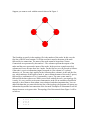
Suppose you want to work with the network showed in Figure 1.
Figure 1. Four node network.
The first thing to specify in the topology file is the number of the nodes. In this case, the
first line of the file must contain a 4. On the next line it must be the name of the node
followed by its connections. The name of the node cannot be larger than 5 letters.
Connections are represented by the number 1. The columns represent the outputs of the
nodes and the rows represent de inputs of the nodes. In the previous example must be 4
columns and 4 rows because there are 4 nodes. For the first row we will proceed as follows:
if the node A receives information (input) from node A (first column) a 1 is placed,
otherwise a 0. The same logic applies for the following three columns. At the end, the first
row, which indicates all the inputs of node A, must contain the name of the node (5 spaces)
followed by a combination of 0 or 1 separated by a space. The same syntax must be
followed for the three other rows. When you are done with all the rows, your topology file
is ready. It is very useful to write some commentaries in the file to remember what kind of
network is, the references from whom it was obtained, and other important data. You can
add all the data that you want after the last line of the topology; the program will ignore any
information beyond the last connection of the last node. Examples of commentaries will be
shown from now on in green color. The topology file of the network from Figure 1 will be
as follows:
4
A
B
C
D
0
1
0
1
1
0
1
0
0
1
0
1
1 Node A has 2 inputs: from B and D
0
1
0
This is my first network.
It has 4 nodes, and every node has two connections.
The first column of the matrix represents all the connections from the first node, the outputs
of A in this case. The second column represents the B’s outputs, and so on. The rows
represent the input connections of each node. You can read this file by row as follows: A
node has not an input from A (the first column is 0), has an input from B (the second
column is1), has not an input from C (the third column is 0), and has an input from node D
(the forth column is 1). Remember that 0 means no connection. Similarly, B node has an
input from nodes A and C, C node has an input from nodes A and C, and D node has inputs
from nodes A and C. This is the topology of the network of Figure 1.
You must keep in mind that the order of the nodes from now on depends of the order of the
nodes in this file. A node will be always the first node, followed by B, which is the second
node, and so on.
It is recommended that you save the topology files with the double extension .top.txt
because that one is the default extension for searching files in the open file dialog window
of Atalia. It allows you to open those files with the default text editor and, at the same time,
Atalia will recognize them as its topology files without changing any default extensions in
your computer.
Syntax of the rules file
The rules of each node must be in a separated file. This file must contain the rules of each
of the nodes from the topology file. You have to be very careful when you make this file.
The nodes must have the same number of entries as were specified in the topology file. For
example, if the node A in the topology file has two input connections (from B and D), the
rules file for the node A must have two columns, each one representing an input node. The
order of the inputs is established, as mentioned before, in the topology file. In our example,
all nodes will have two columns. The rules file must be as follows (remember: comments
are on green):
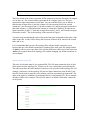
A___________________Columns(input nodes):B,D
00|0
01|1
10|1
11|0
B___________________Columns(input nodes):A,C
00|0
01|1
10|1
11|0
C___________________Columns(input nodes):B,D
00|0
01|1
10|1
11|0
D___________________Columns(input nodes):A,C
00|0
01|1
10|1
11|0
Here are the rules of my first network.
All nodes have the same logical rule: OR exclusive (Ox).
The first row must contain the name of the node (remember, just 5 spaces are allowed).
After this you can write anything you want, a commentary, the program will not read it. For
example, you can add a line and the names of the input nodes for clarity when you create
the file. In the previous example appears a line, never mind, is just design. The next rows
must be filled with all the combinations of the input nodes. As in our example, all nodes
have two inputs, the total number of combinations are four (22=4). Each input combination
must have associated an output, which is the logical rule of the node A. There are 11 spaces
to be filled with the combinations, this imply that the maximum number of inputs of a
particular node is 11. You must respect this situation; the combinations must be right
justified. The output must be always in the 13th column and the separator, the vertical bar
between inputs and output, in the 12th column.
Immediately after the logical rule of node A, comes the logical rule of node B, and so on. In
our example all nodes have the same logical rule: Or exclusive (Ox). In real genetic
examples this is very rare, and the normal condition is that each node has its own different
logical rule.
You can write any comments at the end of the file as in the topology file (texts in green are
comments).
It is recommended that you save the rules files with the double extension .reg.txt because it
is the default extension for searching files in the open file dialog window of Atalia. It
allows you to open those files with the default text editor and Atalia will recognize them as
its rules files, without changing any default extensions in your computer.
Syntax of the asynchrony file (optional)
The asynchrony file specifies the order of actualization of the nodes. Each row specifies the
order of actualization of a particular node. In our previous example, we have a 4 node
network; each row will represent the order of actualization of a node, so you will have 4
rows. Row number 1 refers to the order of actualization of the first node, node A, the row
number 2 represents the order of actualization of the second node, and so on. Again,
remember that the order of nodes depends of the topology file. By default, all nodes will be
actualized at the same time, if you want to specify a different order of actualization, the file
will be like this:
4
3
2
1
Node A will be actualized in 4th place
Node B will be actualized in 3rd place
Node C will be actualized in 2nd place
Node D will be actualized in 1st place
My first asynchrony file.
Order of actualization: D, C, B, A.
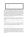
These file tells the program the order of actualization of the nodes. The first node to be
actualized is D, then C, then B, and finally A. You can write comments at the end of the
file. Texts in green are comments.
It is recommended that you save the asynchrony files with the double extension .asi.txt
because that one is the default extension for searching files in the open file dialog window
of Atalia. It allows you to open those files with the default text editor and Atalia will
recognize them as its asynchrony files, without changing any default extensions in your
computer.
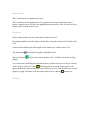
The Network Tab
This section draws the topology of the input network. You can see the network after
reading a topology file in the “Start” tab. You can modify some of its attributes as the labels
and the size of the nodes, as well their fill and edge color. The size of the network and the
width of the connections can be changed too. To restore default values press the undo
button .
If you want to represent a particular configuration in the network's topology (i.e. active
nodes in one color, inactive nodes in another) fill the “configuration” box with a string of
zeros and ones (zeros represent inactive nodes and ones the active ones) and press the brush
button . You can choose the color of the nodes by pressing the active or inactive colored
circles. To restore default values press the undo button .
The topology can be saved with the cactus icon
. Allowed formats are jpg and bmp.
Default values of this tab are:
Sizes box
Labels
Network size
Node size
Lines
On
250
25
1
Colors box
Node color
Line color
Edge color
Red
Black
Black
Configurations box
Active color
Red
Inactive color
Yellow
Example:
Figure 2. Arabidopsis thaliana gene floral network
The Graphic Tab
This tab shows two histograms depicting the sizes of the basins of attraction. The first
histogram graphics their absolute sizes. The second shows the percent of each basin of
attraction.
You can print directly any of them by pressing its corresponding printer button
histogram buttons
wmf.
. The
save the corresponding graphic. Available formats are bmp, emf, and
Example:
Tamaño de la cuenca
Tamaño de las cuencas de los sumideros
3,500
3,500
3,000
3,000
2,500
2,500
2,000
2,000
1,500
1,500
1,000
1,000
500
500
0
0
1
2
3
4
5
6
7
8
9
Sumideros
Figure 3. Basins of attraction absolute sizes of A. thaliana floral network.
10
Tamaño de las cuencas de los sumideros (%)
45
45
40
40
35
35
30
30
25
25
20
20
15
15
10
10
5
5
0
0
1
2
3
4
5
6
7
8
9
10
Sumideros
Figure 4. Basins of attraction relative sizes of A. thaliana floral network.
The Omega Tab
In this tab you will find on the left upper corner a box with the list of all the attractors. The
attractors are numbered consecutively starting from 1. By clicking with the mouse on any
of them, the basin of attraction will be represented graphically. The colors are chosen at
random, each time you modify the graph, colors will change. The attractor will be
positioned at the center of the graphic, if it is a point attractor it will be represented by a
point, if it is a cyclic attractor it will be represented by a circle.
Configurations box
If you want to see the configurations in the graph, you should mark any of the two boxes in
the “Configuration” box. Selecting binary checkbox will display configurations as strings
of zeros and ones; selecting decimal checkbox will convert the string in a 10 base number.
Both are unchecked as default values.
Effects box
The fan button , (turn back arrow icon) changes the angle in which all the configurations
will be arranged. Its default value is 90 degrees. This is useful when the basin of attraction
is very large or complicated. If you diminish the angle the graph will be clearer. Try 0
degrees. This button affects the opening of all the fans, but the center circle.
The magnifier button
zooms in and out the graph. For example, this is useful when the
basin is too large to see a particular configuration. Default value is 1.
Movement box
The x control moves the graph on the x axis.
The y control moves the graph on the y axis upside down. Keep in mind this for the y
button: a negative value will move the graph higher and a positive value will move it lower.
Default values of both controls are 0.
Ratios box
Nodes control modifies the size of the nodes. Default value is 2.
Fan control modifies the radio length of all the fans, except the central circle. Default value
is 50.
Central control modifies the radio length of the central circle. Default value is 50.
The undo button
The cactus button
and jpg.
will redraw the graph with default values.
will save the current graph in a file. Available extensions are bmp
You can keep any modified graph in RAM memory (without saving it in a file) by clicking
on the “Keep it on the list” button
. The image will be stored in memory and it will
appear an identifier name and number on the left lower box list. You can delete any of these
graphs by typing its number in the box at the right of the row button
Example:
and press it.
Figure 5. Basin of attraction of one of the stamens attractors of A. thaliana floral network.
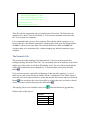
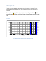
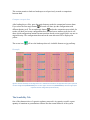
The Monitoring Tab
This section allows following a particular configuration to its attractor. The configuration
may be in decimal or in binary format. You must select what type of configuration will be
typed in the Configuration box by checking the corresponding box. Finally press the
monitoring button . An image consisting of red and blue squares at the right of the screen
will be displayed. Each square represents a node and its color the state of that node, blue
signifies inactive and red active. Each row of squares represents a particular configuration.
The uppermost row is the input configuration, below this one a set of configurations will be
showed, each one represents the next configuration at time t+1, and eventually, when color
do not changes or changes in a cyclic form, an attractor will be reached.
The cactus icon
and bmp.
will save this set of colored configurations. Available formats are jpg
Example:
Figure 6. Scanning of configuration 0000000000000 until it reaches an attractor (1100110101100).
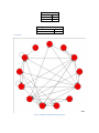
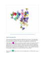
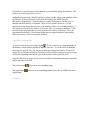
The Neighborhoods Tab
In this section you can perform an analysis of small perturbations to any configuration and
calculate the stability of an attractor or any other configuration. The input configuration can
be read in binary or decimal formats. After giving it, press the “Neighbors” button to start
de analysis. On the left panel the results will appear in text format. The analysis consists in
change the state of each node, one by one, and recon its destiny attractor. On the right you
will find the results in a graphic form. The graph shows a central node which represents the
original configuration painted with the color of its attractor. The surrounding nodes
represent what happens if that node changes its state, if the destiny is the same, the color of
the node will be the same as the central node, and otherwise the color will be different. The
stability of the node will be calculated on the basis of small mutations at a Manhattan
distance equals to 1. A node with 100% of stability at that range of perturbation will show
all the nodes with the same color as the central node.
The sizes box controls the graphic style.
Names checkbox allows showing or hiding the labels of the nodes. Its default value is
checked.
Network control modifies the size of the entire graph. Its default value is 250.
Nodes control changes the size of all the nodes of the graph. Its default value is 50.
Lines control modifies the width of the connecting lines of the network. Its default value is
1.
As in the Omega tab section, you can keep any modified graph in RAM memory (without
saving it in a file) by clicking on the “Keep it on the list” button
. The image will be
stored in memory and it will appear an identifier name and number on the left lower box
list. You can delete any of these graphs by typing its number in the box at the right of the
row button
Fox button
Example:
and press it.
saves the graph into a file. Available formats are jpg and bmp.
Figure 7. Stability of sepal attractor of A. thaliana floral network. Mutations on AP1, TFL1, AG, WUS, AP2 genes will
lead to the same attractor. Mutation of LFY will change the destiny of the configuration.
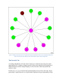
The Derrida Tab
According to Kauffman (1991) the chaotic behavior of a Boolean network persists until
approximately K=3 (number of inputs per node). Below this connectivity the properties of
random Boolean networks change abruptly, now the networks exhibit unexpected and
collective order.
Derrida curve is a way to determine this transition phase between chaos and order. Slopes
greater than 1 implies that two very similar initial conditions diverge exponentially in time,
characteristic of a chaotic phase, in contrast with an ordered regime which has a slope
lower than 1.
The Derrida curve can be calculated with all possible configurations of the network, but for
some sizes, this can be very time consuming. In order to explore this time, it is possible to
perform the analysis with a sample of configurations. The “Total box” performs the
complete analysis, just press the corresponding magic button . If you want to explore
times of calculation, use the sample box. Type the size of the sample in the “Sample size
box” and press the corresponding magic button .
The printer button
The graph button
will print the graph.
will save the graphic into a file. Available formats are jpg and bmp.
Example:
Curva de Derrida
13
12
11
10
9
8
7
H(t+1)
6
5
4
3
2
1
0
0
2
4
6
8
10
12
H(t)
Figure 8. Derrida curve obtained for the A. thaliana floral network with a sample size of 100.
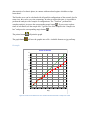
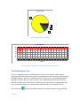
The Landscapes Tab
The omega space is difficult to analyze, unless for very small networks, due to its huge set
of configurations. There are no methods to do this because it is not clear what to analyze
either. Atalia has some visual analysis to explore the Omega space. In this section it is
possible to represent the Omega space in three different ways: the destinies mosaic, the
Manhattan distances mosaic and the topological distances mosaic. In all of these mosaics
each configuration is represented by a square. The color of each square represents
respectively the destiny configuration (its corresponding attractor) of that particular
configuration, the topological and the Manhattan distances to its attractor.
It is possible to compare two landscapes and to obtain a final landscape showing the
differences between them. This is useful in order to observe the effects of certain mutation
or alteration in the logical rules of the network.
The mosaic represents in biological terms the morphospace over the genetic configurations,
the space FOGC (space of Forms Over Genetic Configurations).
Landscapes box
Point attractors. By clicking on it the mosaic will mark in blue those configurations
(squares) that are point attractors.
Cyclic attractors. Clicking this option the mosaic will mark with different colors those
configurations (squares) that are cyclic attractors.
Topologic distance. This option colors each configuration (square) according to its
topological distance to its corresponding attractor.
Manhattan distance. Selecting this option will color each configuration (square) according
its Manhattan distance to its corresponding attractor.
Destiny (Epigenetic landscape). Clicking on this option each configuration (square) will be
colored according to its final destiny (attractor).
Save file box
This selection will save the data of the landscape showed on a file. It will not save the
image.
Load files box
This section permits to load two landscapes saved previously to make a comparison
between them.
Compare carpets box
After loading the two files, press the magic button to make the comparison between them.
If you select the first magic button
the result will show just the configurations with
different destiny (red). The second magic button
makes the comparison more subtle. Its
results will show how many configurations have attained a new attractor (red), but it will
show which configurations attained an attractor that already exists (purple) but it was not its
original destiny. The configurations that end on the same attractor will be displayed in
yellow.
The cactus icon
will save the landscape showed. Available formats are jpg and bmp.
Example:
Figure 9. Destinies landscape of all configurations of A. thaliana floral network. The uppermost left square represents
the first configuration (0000000000000), the one at its right is the next one (0000000000001). The lower right square
represents the last configuration (1111111111111).
The Sensibility Tab
One of the characteristics of a genetic regulatory network is its capacity to tackle a great
quantity of mutations or perturbations without alter the normal behavior of the system.
Nevertheless, is possible that certain mutations or perturbations change this behavior. This
property gives the opportunity to evolve.
Atalia allows performing a detailed analysis of all the possible single point mutations of the
logical rules of the network and classify them according to the IRON (Intrepid,
Reactionary, Opportunistic, Neutral mutations) regime. Each output of all the rules is
changed and the dynamics is calculated. There are four possible scenarios. 1) If the
mutation does not change the attractors or the number of them, it is a neutral mutation. 2)
The mutation just reduces the number of attractors. This is a reactionary mutation. 3) The
mutation keeps the original attractors and increases the number of attractors. This is an
opportunistic mutation. 4) The mutation diminishes de original attractors, but generates
other new attractors. This is an intrepid mutation.
Sensibility analysis box
To start the analyses press the magic button . This test cans last very long depending on
the number of nodes and the number of inputs of each one. To see the effect of changing
the output of a specific rule, you can browse them by selecting the number of row of the
output. The row scanner will show what kind of effect will have changing a specific output
with its corresponding node and the type of the mutation with a particular color.
After the analysis four graphs will be shown with different information about the mutations
and the attractors recovered.
The printer button
The graph button
jpg and bmp.
Example:
will print the corresponding graph.
will save the corresponding graphic into a file. Available formats are
Regimen IRON
N
I
R
O
Figure 10. Mutation types percentage
Sensibilidad
100
80
60
40
20
0
20
40
60
80
100 120 140 160 180 200 220 240 260 280 300 320 340 360 380
Salida #
Figure 11. Number of attractors recovered according to the mutated output.
The Morphospace Tab
This is a complement to the sensibility analysis. It shows in a mosaic, whose squares
represent a particular configuration, which configurations are attractors after performing the
sensibility analysis. There are 3 possible outcomes. The first one is configurations that are
originally attractors, they are colored in blue. The configurations that are new attractors
under the mutations are colored in red. The third and last possibility is configurations that
never are attractors under any of the possible mutations, they are presented in white.
The cactus icon
Example:
will save the landscape showed. Available formats are jpg and bmp.
Figure 12. Original attractors (blue) and new attractors (red) after mutating each one of the outputs.
Glossary
Attractor: Certain configuration or group of them once attained the system will stay there
forever. An attractor conformed by just one configuration is called a point attractor,
otherwise it is a cyclic attractor and the number of configurations that conforms it are its
period.
Basin of attraction: Set of all configurations with the same destiny attractor.
Configuration: A particular set of states from all the nodes of the network.
Eden: Configuration with no previous configuration at time t-1. Without any perturbation,
the only possible way to attain an Eden is to start in one (Wuensche 2002)
Epigenetic landscape: Metaphor proposed by C. Waddington (1940) in which the fate and
the routes of differentiation of a cell are represented by a downhill landscape. The cell is a
ball that travels through this rugged surface and finally attains a stable place on it: its final
cellular type.
Genetic regulatory network (GRN): Abstraction of a genetic system with a network
model.
Hamming distance: The number of bits which differ two binary strings. Hamming
distance can be seen as Manhattan distance between bit vectors.
Manhattan distance: The distance between two points measured along axes at right
angles.
Morphospace: The set of all possible forms or varieties of a structure or character can
have, either real or in theory. Word proposed by D. Raup (1966).
Omega space: The set of all possible configurations of a network. For example, a 5 node
binary network has an omega space equal to 25=32 configurations.
State: Nature of a node at a particular moment. For example, a binary node can only have
two states: 0 or 1.
Transient: Configuration which has at least one previous configuration (it is not an Eden),
and has at least one successor configuration (it is not an attractor) and does not conforms
part of a cyclic attractor.
Stability: The degree of resistance an attractor can suffer (alterations in its configuration)
and return to itself. A measure of how strong is an attractor to perturbations. An attractor is
an equilibrium point; its stability depends on its capacity to return to itself after being
modified.
References and bibliography
Álvarez-Buylla ER, Chaos Á, Aldana M, Benítez M, Cortes-Poza Y, et al. (2008) Floral
Morphogenesis: Stochastic Explorations of a Gene Network Epigenetic Landscape. PLoS
ONE 3(11): e3626. doi:10.1371/journal.pone.0003626
Chaos Á, Aldana M, Espinosa-Soto C, García Ponce B, Garay A and Álvarez-Buylla E.
(2006) From Genes to Flower Patterns and Evolution: Dynamic Models of Gene
Regulatory Networks. Journal of Plant Growth Regulation 25:278-289
Espinosa-Soto C, Padilla-Longoria P, Alvarez-Buylla E. (2004). A gene regulatory network
model for cell-fate differentiation during Arabidopsis thaliana flower development that is
robust and recovers experimental gene expression profiles. Plant Cell 16:2923–2939.
Monod J and Jacob F. (1961). General conclusions: Telenomic mechanisms in cellular
metabolism, growth, and differentiation. Cold Spring Harb. Symp. Quant. Biol. 26, 389–
401.
Kauffman SA. (1969). Metabolic stability and epigenesis in randomly constructed genetic
nets. J Theor Biol 22:437–467.
Kauffman SA. (1991) Antichaos and adaptation. Sci. Amer. 265(2):64-70
Kauffman SA 1993. The origins of order: self-organization and selection in evolution.
Oxford University Press.
Raup D.M. (1966). Geometric analysis of shell coiling: general problems. Journal of
Paleontology 40: 1178-1190
Waddington, C. H. (1940). Organisers and Genes, Cambridge University Press.
Wuensche A. (2002). Basins of Attraction in Network Dynamics: A Conceptual
Framework for Biomolecular Networks, in "Modularity in Development and Evolution",
eds G.Schlosser and G.P.Wagner. Chicago University Press 2004, chapter 13, 288-311.
(Santa Fe Institute working paper 02-02-004, 2002).