Download Masters Thesis.docx - University of Washington

A Study of Fluid Sloshing in a Cylindrical Fuel
Tank with Use of a Laser Scanning System to
Capture Fluid Motion and Coupled EulerianLagrangian Analysis for Simulation
Benjamin D. Speirs
A thesis submitted in partial fulfillment of the requirements for the degree of
Master of Science in Mechanical Engineering
University of Washington
2013
Committee:
Per Reinhall (Chair)
Alberto Aliseda
James Riley
Mark Van Sickle
Program Authorized to Offer Degree:
Mechanical Engineering
© Copyright 2013
Benjamin D. Speirs
University of Washington
Abstract
A Study of Fluid Sloshing in a Cylindrical Fuel Tank with Use of a Laser Scanning System to
Capture Fluid Motion and Coupled Eulerian-Lagrangian Analysis for Simulation
Benjamin D. Speirs
Chair of Supervisory Committee:
Professor Per Reinhall
Mechanical Engineering
A study was conducted to gain a better understanding of fluid structure-interaction when fuel
sloshes inside a cylindrical tank. The study involved building a test fixture to create sinusoidal
motion which induced sloshing inside a partial fuel tank section. Strain gauges were installed on
the tubing inside the tank that was used to draw and return fluid from and to the tank. A multicamera video capture system was used to record fluid motion which was illuminated using a
grating of laser lines arranged in an alternating color pattern. A software program was
developed to convert the captured video into 3D data representing the free surface of the fluid.
A finite element model was created and a coupled Eulerian-Lagrangian analysis was performed
to recreate the test conditions in simulation. When the results of the test and simulation were
compared, the fluid motion was found to match favorably. However, the strain time history
recorded from the test, when compared with that of the simulation, was found to have less
favorable correlation. Possible sources of the discrepancy are discussed and potential
improvements are proposed which may improve the correlation of the simulation to the test.
Table of Contents
Chapter 1: Introduction ................................................................................................................................ 1
Chapter 2: Objectives.................................................................................................................................... 4
Chapter 3: Experimental Setup ..................................................................................................................... 5
Overview of the Test Fixture..................................................................................................................... 5
Fuel Tank Section and Draw/Return Tube Assembly ................................................................................ 5
Main Fixed Base and Moving Shuttle........................................................................................................ 9
Electromechanical Components of The Test System ................................................................................ 9
Video Cameras and Lasers System.......................................................................................................... 13
Working Fluid .......................................................................................................................................... 18
Chapter 4: Fluid Surface Scanning .............................................................................................................. 19
Background ............................................................................................................................................. 19
Overview of the Software ....................................................................................................................... 20
Camera Calibration ................................................................................................................................. 21
Reference Target Points.......................................................................................................................... 23
Video Capture ......................................................................................................................................... 25
Laser Line Processing .............................................................................................................................. 27
Perspective Transformation.................................................................................................................... 32
Triangle Tessellation and Data Export .................................................................................................... 34
Visualization of the Scanned Result ........................................................................................................ 36
Accuracy & Final Comments ................................................................................................................... 37
Chapter 5: The Finite Element Model & Simulation ................................................................................... 39
Introductory Discussion .......................................................................................................................... 39
The Lagrangian Mesh .............................................................................................................................. 40
The Eulerian Mesh .................................................................................................................................. 43
Initial Fluid Position................................................................................................................................. 45
Contact and Fluid Structure Interaction ................................................................................................. 45
Material Definitions ................................................................................................................................ 46
Boundary Conditions and Loading .......................................................................................................... 47
Output ..................................................................................................................................................... 48
Computational and Other Considerations .............................................................................................. 48
Chapter 6: Results ....................................................................................................................................... 49
Event Descriptions .................................................................................................................................. 49
Displacement and Acceleration Time History ......................................................................................... 50
Strain Time History and Spectral Analysis............................................................................................... 55
Free Surface Fluid Motion....................................................................................................................... 58
Chapter 7: Discussion .................................................................................................................................. 65
Displacement and Acceleration .............................................................................................................. 65
Input Force from the Electromechanical Drive ....................................................................................... 65
Strain response ....................................................................................................................................... 67
Free Surface Fluid Motion....................................................................................................................... 71
Chapter 8: Conclusion ................................................................................................................................. 73
Acknowledgements..................................................................................................................................... 75
References .................................................................................................................................................. 76
Appendix A: Strain Gage Installation on Draw/Return Tubing ................................................................... 77
Appendix B: Laser Module Alignment and Wiring Diagram ....................................................................... 79
Appendix C: Investigation of Excessive Vibration in the Electromechanical Drive System ........................ 82
Appendix D: Normal Modes Analysis .......................................................................................................... 88
Chapter 1: Introduction
The fuel storage tanks, tubing, and transfer lines that deliver fuel to the engine of a large truck
are critical to the efficiency, environmental compliance, and power of the vehicle. Since heavy
trucks are frequently operated in rough terrain, often under continuous use, and are expected to
run for more than a million miles of operation in highway use, it is important that the fuel
systems are durable and reliable. Figure 1 shows a Class-8 heavy truck with cylindrical fuel tank
with a typical mounting configuration on the chassis frame rail below the cab.
Figure 1. A polished aluminum cylindrical fuel tank installed on a Class-8 Heavy Truck. Cab access steps are
mounted to the exterior of the tank. The large black plastic tank located behind the fuel tank is for diesel exhaust fluid
(DEF) used in aftertreatment.
Components inside the fuel storage tank are not only subjected to vibration from rough road
inputs, but they can also see significant loading and stress due to the sloshing motion of the
fuel. One such component in a fuel tank is the tubing that is used to draw the fuel from the tank
and then return any excess fuel back to the tank. The purpose of this draw and return fuel “loop”
is to provide the truck’s engine with sufficient fuel at all times. More fuel than actually required is
pumped to the engine and any excess fuel is returned back to the tank which allows the engine
to quickly increase power output without lagging or stalling while otherwise waiting for more fuel
to arrive at the engine. This results in smooth acceleration and efficient operation. A side effect
of this fuel loop, however, is that the fluid inside the lines becomes heated by thermal radiation
1
from the adjacent hot surfaces of the engine and from heat conduction where the fuel lines are
attached to the hot engine.
Optimal combustion in the truck’s engine is achieved by balancing the output power, fuel
efficiency, and output byproducts (soot, carbon oxides, nitrogen oxides, etc). Achieving optimal
combustion requires a low fuel temperature. Upon returning the fuel back to the tank it is
required to do so in such a way that the heated fuel is mixed with the relatively cool fuel in the
tank as shown in Figure 2.
Figure 2. Fuel that is drawn from the tank is relatively cool compared the heated fuel returning from the engine. It is
advantageous to have the hot fuel mix with the cooler fuel in the tank before having it pulled back up to the engine.
A combined draw and return tubing assembly, where the two tubes are attached to a common
mounting plate, is an effective design that requires only a single access hole in the fuel tank for
installation. The combined “draw/return” unit, shown in Figure 3, is the component that was of
primary interest in this study. It features an elongated segment on the draw tube which pulls the
fuel from a cool location in the tank, and a pinched end on the return tube which causes the
returning fluid, which is of a higher temperature, to be accelerated to a high velocity in the
opposite direction. The two tubes in this assembly are welded to a mounting plate and welded
together where they cross over each other at the bottom.
2
Figure 3. A combined draw and return tube assembly. The larger diameter tube with the extended section pointing
down toward the table is the “draw” tube. The smaller diameter tube with the “pinched” end pointing up is the “return”
tube.
Being able to properly design the component shown in Figure 3 for durability of was the
motivation of this research.
3
Chapter 2: Objectives
A good understanding of the conditions resulting from fluid sloshing in a fuel tank is required in
order to effectively design internal fuel tank components. With the knowledge and
understanding of these conditions, an accurate simulation can be developed to model the
physical response.
To support the statement above, the following objectives were established for the research
work:
1. Design and build a test fixture capable of producing lateral sloshing in a fuel tank.
2. Develop and install a data acquisition system that captures strain, displacement, and
video.
3. Develop a software program to process the video captured on the test fixture and
convert that video data to a representation of the free surface of the fluid.
4. Create a finite element model that accurately simulates the test conditions.
5. Compare the test and simulation results and identify the important parameters of the
simulation that are needed to provide an accurate representation of the physical
response.
4
Chapter 3: Experimental Setup
Overview of the Test Fixture
In order to study the effect of fluid sloshing in a lateral motion (a motion that is, in effect, left-toright and perpendicular to the axis of the cylindrical tank) an oscillation test fixture was
developed. The following sections of this chapter describe the major components and systems
of the test fixture created for this research work.
Fuel Tank Section and Draw/Return Tube Assembly
A fuel tank was salvaged from a heavy duty truck that had been taken out of service after
reaching the end of its service life. As such, there were a few dents and scratches, but overall
the component was in good condition. The original internal volume of the tank was 380 liters
(100 gal), with an overall length of 1270 mm. The material of the tank was a 5052 Aluminum
alloy with a nominal wall thickness of 3.2 mm. The internal diameter of the tank was 620 mm
and had been produced by roll forming then joined by seam welding. The ends of the tank had a
slight crown, or dome feature, and were attached to the tank with an external weld.
To adapt the tank to the testing fixture, the tank was cut perpendicular to the cylindrical axis,
effectively shortening the tank to 560 mm with a resulting internal volume of 167 liters. At the
cut-off location, an external flange was welded in place to accept a transparent cover. The
modified tank is shown in Figure 4.
5
Figure 4. The modified tank that had been shortened and had an external flange welded in place. In the figure, the
draw/return assembly is loosely placed into an access hole in the top surface of the tank. Wiring for strain gages that
were installed on the draw/return tubes is visible in the image.
A 700 mm diameter round cover was fabricated from a 10 mm thick piece of clear acrylic plastic.
To secure the cover to the tank, 24 equally spaced M6 bolts were installed around the perimeter
attaching it to the newly added flange. To seal the cover to the tank’s flange, a closed-cell foam
tape was used between the aluminum and acrylic material. The installed cover is shown in
Figure 5.
The acrylic material had been selected for the cover due to its superior optical transmissibility
and resistance to surface scratching. However, one shortcoming of acrylic is how brittle it is
compared to an alternative such as polycarbonate: during initial assembly, one of the
attachment bolts was over tightened which resulted in a small crack in the cover. A stress relief
hole was drilled at the end of the crack tip and the cover was re-oriented to place the crack
outside of the camera’s field of view and above the fluid fill level. These efforts were successful
and the damage did not impact the testing.
6
Figure 5. The clear acrylic cover installed on the tank flange. The crack in the cover is indicated. Partly visible in the
upper left corner of the image is the access hole through which the draw/return assembly was inserted.
The draw/return tube assembly that was part of the original tank was discarded. A new unit was
acquired and instrumented with four uniaxial strain gages. The detail for the strain gages
installed on the tubing is included as Appendix A.
A new 120 mm diameter access hole was cut into the upper surface of the tank allowing
insertion and placement of the new draw/return unit. Rather than weld the draw/return assembly
in place, as the original was, the new unit was affixed using six M6 bolts and threaded inserts on
the tank wall. This allowed for easy installation and removal during testing. The bolted
installation is shown in Figure 6, with a comparison to the original.
7
Figure 6. The image on the left shows the original installation with perimeter weld on the connector flange of the
draw/return assembly. The image on the right shows the bolted connection used on the test fixture. Wiring for the
strain gages is routed through the small hole in the connector flange (trimmed with blue tape).
The draw/return tube assembly and the interior of the tank were painted a dark gray color
(Figure 7) to reduce reflection of light during the video capture, which is described in Chapter 4.
Without the gray paint, the natural surfaces of the aluminum components were almost mirrorlike when wet, making video capture difficult.
Figure 7. Inside surfaces of the tank and tubing painted dark gray to reduce the amount of reflected light from the
originally shiny aluminum surfaces.
8
Main Fixed Base and Moving Shuttle
A sturdy fixed base was fabricated from plywood and framing lumber. The base was leveled and
bolted to a concrete floor. On top of the fixed base, two corrugated steel rails were attached.
Each steel rail provided mounting points and load transfer for three shaft supports to hold an
1180 mm long, 25.4 mm diameter steel shaft.
A shuttle was built to support the moving fuel tank section. It was fabricated primarily from
plywood and aluminum materials in order to keep the moving mass of the test system as low as
possible. On the underside of the shuttle, two aluminum rails were installed along with pillow
blocks containing linear bearings which rode on the steel shafts of the fixed base. Aluminum
gussets were added to provide rigidity as well as anchorage points. The fuel tank section was
supported by six elevator bolts which allowed for its leveling and alignment. The tank section
was held in place with two nylon ratcheting straps and adhesive tape to prevent rotation. The
shuttle mounted on the base is shown in Figure 8.
Figure 8. The moving shuttle (orange) carries the test section of the fuel tank atop linear bearings. Bearing shafts are
mounted to the rigid base (blue) by way of steel rails.
Electromechanical Components of The Test System
During the initial system design, several design options were evaluated, including hydraulic and
pneumatic cylinders, a ball screw driven by servo control, and a system of chain and sprockets.
9
The final design selection was that of an electric motor and worm gear speed reducer driving a
mechanical crank attached to a connecting rod. The benefit of the selected system as compared
to alternatives was the simplicity of motion control. While some of the other systems evaluated
would require position feedback and control software, the simpler crank and connecting rod
setup provided “built in” control for sinusoidal motion. A shortcoming of this type of system,
however, is that it can only do sinusoidal motion. For the purpose of this research, this limitation
was not an issue. The electromechanical drive used on the fixture is shown in Figure 9. To
accommodate the drive system to the test fixture, a fabricated aluminum armature was
constructed. This was bolted to the side of the fixed base as well as being bolted to the concrete
floor.
Figure 9. The electromechanical drive attached to the side of the oscillation test fixture.
The electric motor used for the system was a 1 kW 220V 3-phase AC induction motor. Motor
speed control was provided by a 1.5 kW variable-frequency drive (VFD). This combination
allowed the test events to be set at a desired motor speed with the VFD providing sufficient
power to maintain a nearly constant oscillation frequency. Mated to the electric motor was an
electromagnetic brake and clutch unit. This provided capability for automated start and stop of
the test events. The output of the brake/clutch unit was attached to a 40:1 worm gear speed
reducer. The motor speed was rated at 1800 revolutions per minute (RPM), resulting in a top
10
oscillation rate for the shuttle of 45 cycles/minute (0.75 Hz). Figure 10 shows the motor,
brake/clutch unit, and gearbox.
Figure 10. A posterior view of the test fixture showing components of the electromechanical drive train. From left to
right are the electric motor, electromagnetic clutch/brake unit, and the 40:1 worm gear speed reducer.
The output shaft of the worm gear speed reducer was fitted with a steel disc, shown in Figure
11, which acted as an offset crank. A row of pre-drilled holes in the crank disc provided fixed
points where a connecting rod could be attached. The connecting rod was a 1270 mm long
hollow aluminum tube with ball joints at each end. The other end of the connecting rod was
attached to the moving shuttle which supported the fuel tank test section. An in-line axial force
transducer was used at the connection of the rod to the shuttle to record the load time history for
the test event.
11
Figure 11. The offset crank disc with holes for setting the stroke length. The connecting rod, shown in the image, is
set for 350 mm of stroke length. The white arrows on the disc provide an alignment reference for positioning the disc
at the beginning of a test.
After initial testing, unwanted vibration was noted in the drive train. This presented as a
pulsation in the force data signal. Also noted was excessive backlash (free play) in the worm
gear speed reducer. This was identified after a review of the displacement signal showed
sudden “jumps” when the drive mechanism changed between pushing and pulling on the
shuttle. A set of nylon friction cords, shown in Figure 12, were tensioned using an extension
spring and were wrapped around the offset crank disc to provide a braking action on the disc.
This braking force put a more continuous load on the electric motor which helped reduce some
pulsation in the output force of the connecting rod. Also shown in Figure 12 is the addition of
structural bracing to the concrete wall to the rear of the test fixture. These efforts were only
partially successful at reducing the undesired input pulsation. Additional discussion and
information regarding the input force pulsation is included in Appendix C.
12
Figure 12. The spring-tensioned nylon braking cords are shown wrapped around the crank disc. The added structural
bracing to the back wall can also be seen.
Video Cameras and Lasers System
Two camera mounting positions were created using thin-wall aluminum tubing in a tripod
configuration, shown in Figure 13. The tripods were rigidly connected to the moving shuttle. The
camera mount positions were approximately 200 mm above the horizontal center line and
spaced 500 mm away from the clear acrylic cover. The lateral offset of the two cameras from
the center line was, respectively, 250 mm to the left and right resulting in 500 mm spacing
between the two mounts. A ball swivel connection was used with a standard camera mount ¼”20 screw. The position of the camera mounts provided a downward-looking view into the tank.
Figure 13. The two tripod camera mounts. The left image shows the side view, while the right image shows a top
down view of the camera mounts. The tripods are connected to the moving shuttle (orange component).
13
Two Logitech C920 USB cameras were used to capture video at 1280 x 720 resolution and 30
frames per second. While these “consumer-grade” cameras were originally solely intended to
provide a proof of concept for video capture, they performed well enough that they were used
for the duration of the testing. Detail of the camera mount is shown in Figure 14.
Figure 14. One of the C920 USB cameras mounted to a tripod. A ball swivel allowed the camera to be adjusted to
capture the area of interest inside the fuel tank.
To illuminate the surface of the fluid, an array of 14 laser lines was used. The array was
arranged in an alternating pattern of blue (420 nm, 5 mW) and red (650 nm, 5 mW) laser
modules outfitted with optical lenses producing lines with a 120 degree fan angle. These were
evenly spaced 37 mm apart and oriented perpendicular to the axis of the cylindrical tank. The
individual 12 mm diameter by 30 mm long laser modules were mounted to a machined
aluminum block, which is shown in Figure 15. The mounting block was attached to the outside
of the tank at the top and slightly off-center using two M6 bolts. A row of 16 mm diameter holes
was drilled in the surface of the tank to allow the laser light to shine in from the outside. This
exterior mounting position allowed a wide spread of the laser lines, as well as providing some
protection of the laser modules from fluid splashing. After the modules were aligned and
checked for perpendicularity to the fuel tank’s central axis, they were fixed in place with a set
screw and a few drops of hot melt adhesive.
14
Figure 15. The laser mounting block attached to the exterior of the tank.
Data Acquisition System and Control System
Two portable laptop computer data collection systems were used. The first system was used to
capture video data from the two cameras. This video capture system is described in detail in
Chapter 4. The second data collection system utilized a National Instruments compact data
acquisition chassis (NI cDaq-9172). Shown in Figure 16, the data acquisition chassis was fitted
with two strain bridge modules (NI 9237) and one analog voltage module (NI 9239).
15
Figure 16. The compact data acquisition unit (cDAQ) used for data collection with three modules inserted. The left
module has inputs from the force transducer and linear potentiometer. The center module has inputs from the four
strain gages on the draw return tube. The right module has the voltage input from the clutch circuit.
Four channels of strain data were collected from gages installed on the draw/return tube
assembly. One channel of force data was collected from the load cell attached between the
connecting rod and the moving shuttle. One channel of displacement data was collected from a
linear transducer mounted between the shuttle and the motor armature. The analog voltage
module was used to monitor the actuation of the clutch/brake unit, which acted as a software
“trigger” to start the logging of data. The data collection rate was 1000 samples/second using
National Instruments Signal Express software.
A custom electronic control panel was built for the test fixture. The panel allowed for automatic
and manual control of the brake/clutch unit. In manual mode, the control panel provided
operation of the unit allowing movement of the shuttle so that it could be staged in the correct
starting position for the next upcoming test event. In automatic mode, the control panel used a
digital timer with electronic relays to control the clutch and brake operations. For a test event,
the timer was programmed with “On” and “Off” times for clutch and brake operations. The
programmed event was started with the push of a button. The control panel and two laptop data
collection systems are shown in Figure 17.
16
Figure 17. The two laptops for data collection and the control panel in the middle. A data collection event is being
demonstrated. During an actual event, the ambient lighting would be reduced completely for best results with the
video capture system.
The sequence below describes a typical data collection event:
●
●
●
●
●
●
●
●
Move the shuttle to the initial location using the manual controls.
Set the “On” time for the clutch (e.g. 4 seconds).
Set the “On” time for the brake (e.g. 5 seconds).
Set the control panel to automatic mode.
Activate data collection of the Signal Express software.
Set the motor speed (in RPM) on the VFD control keypad (e.g. 1200 RPM) and wait for
the motor to come up to speed.
Start the video capture software.
Push the start button on the automatic control.
With the example settings given in the sequence above, the following would occur:
●
●
●
●
The electronic timer closes the clutch relay sending 90 V DC to the electromagnetic
clutch.
The clutch voltage signal is detected by Signal Express which starts the data logging.
With 40:1 reduction through the worm gear, the crank disc begins to turn at a constant
30 RPM (0.5 Hz).
The clutch stays engaged for 4 seconds during which time the shuttle makes two
complete strokes.
17
●
●
The timer opens the clutch relay and closes the brake relay sending 90 V DC to the
electromagnetic brake. The brake is applied stopping the shuttle, and holds it in place for
5 seconds.
When the clutch voltage drops, the Signal Express software is triggered for shut down. It
was typically set to continue recording an additional 5 seconds of data after the
shutdown trigger was detected.
Working Fluid
In place of diesel fuel, an alternative working fluid was chosen for purposes of safety and
convenience. The fluid used was a mixture of ordinary “tap” water and reduced-fat milk (2%
milkfat). The addition of milk to the fluid was used as a dye to provide a reflective property to the
surface of the fluid. This allowed the cameras to capture the light projected from the laser line
modules. A study was done to identify an optimum milk-to-water ratio. The ideal concentration
was found to be 1 part milk to 7 parts water: a 12.5% solution of milk by volume. Table 1 shows
the comparison of fluid properties.
Table 1. Comparison of relevant fluid properties.
Water
Milk
Working Fluid
(87.5% Water+12.5% Milk)
Diesel Fuel
Density (kg/l)
0.99911
1.02982
1.0029
0.87603
Kinematic Viscosity
(mm2/s)
1.1214
2.0095
1.232
4.06
As shown in the above table, the density of the working fluid is 14.5% greater than diesel fuel.
As a result, the heavier working fluid was expected to impart slightly higher inertial loads on the
draw and return tubing than if diesel fuel had been used in the test. In contrast the kinematic
viscosity of the working fluid is 69.2% less than diesel fuel. Due to the fluid velocities anticipated
in the test events, viscosity was expected to have little effect. Based on the comparison of
density, and expectation of low viscous loads, the working fluid is seen as a good surrogate for
diesel fuel. It also has the significant benefit of being non-flammable and chemically compatible
with other components of the test equipment.
1
http://en.wikipedia.org/wiki/Density
Measured
3
http://www.usor.com/files/pdf/5/ULSDspec.pdf
4
http://en.wikipedia.org/wiki/Viscosity
5
http://download.journals.elsevierhealth.com/pdfs/journals/0022-0302/PIIS0022030284814174.pdf
6
http://www.microhydraulics.com/LEEWEB2.NSF/1c6397740f8b45e1852563b9006d6bc6/
2
18
Chapter 4: Fluid Surface Scanning
A major objective of this research was to gain a better understanding the fluid motion when it
sloshed around in the tank and how that motion produced loads on the draw/return tube
assembly. During the initial planning it was decided to use video cameras to capture the test
event for comparison to the simulation model. While the video by itself would be beneficial for
confirming that simulation model was generally behaving similar to the test conditions, this
comparison alone was too subjective. A method to objectively measure the fluid as it moved
inside the tank was required. A review of literature related to fluid measurement techniques
produced several potential alternatives which were investigated: Particle Image Velocimetry
(PIV), Laser Doppler Velocimetry (LDV), Acoustic Doppler Velocimetry (ADV), image refraction,
and free surface scanning.
The approach selected for this research was a technique which used laser line scanning to
capture the free surface motion of the fluid. This would provide a measurable result that could
be objectively compared to that of the simulation.
Background
Initial inspiration for scanning the free surface of the fluid came from Bateman et al. (2006),
where they describe a method using parallel laser lines and video cameras to capture the
surface profile for comparison to simulation results. The experimental subject of that research
involved a flume dam break followed by free flow onto an empty platform. Their system was an
open, visibly unobstructed domain from the camera’s viewpoint, which differs from the closed
fuel tank container in this research study. While this difference was seen to present some
challenges for the present research, their technique was appealing because of the large surface
area that could be observed.
A search for existing software code was conducted, with a preference to find an open source
free-to-use, or a low cost solution. A few open source laser scanner software codes were found,
but none were seen suitable for immediate use, and would require significant customization or
total re-write. Some commercial software products were also investigated, but they also
appeared to have a significant amount of customization required and were cost prohibitive
considering the available budget of this research project.
19
During the search for available code, an online project called OpenCV (http://opencv.org) was
found. The OpenCV project appeared to have an active community of developers and users and
a number of existing reference codes for image and video capture that could be used as a
starting point for developing custom code for this research work.
The following sections of this chapter outline the custom software code that was developed for
this research study. This custom code project is available online for review and use by anyone
with interest and is hosted at: http://code.google.com/p/slosh-test/
Overview of the Software
The software program created for this research, named “Slosh-Test,” is organized as a test
manager. It is set up as a linear progression of activities that are required to capture video on
the fuel tank test fixture that was described in Chapter 3, and convert that video information to
3D data representing the free surface of the fluid.
The software program allows video input from two cameras simultaneously, but it should be
noted that the cameras are not a stereoscopic pair. The use of multiple cameras was done to
provide a wide field of view with some overlap of the scanned region. This gives the system
some redundancy and coverage of the area that would be obscured by the draw/return tubing if
only a single camera had been used.
Slosh-Test provides a graphical user interface where test events can be set up and documented
as laboratory testing progresses. As each new event is created, an organized set of file storage
folders are created to save the video data and the resulting processed files.
The software makes use of the pinhole camera mathematical model, shown graphically in
Figure 18. The pinhole camera model is described with great detail in the Bateman paper as
well as sources such as the Wikipedia article7 devoted to the topic and on the OpenCV Project’s
documentation site8. With those sources available, this paper is primarily devoted to the material
that is unique to the present research work, and as such leaves out some of the detail.
7
8
http://wikipedia.org/wiki/Pinhole_camera_model
http://docs.opencv.org/modules/calib3d/doc/camera_calibration_and_3d_reconstruction.html
20
Figure 18. A diagram showing the concept of the pinhole camera model. The scene of the tree is projected through a
virtual point on to an image plane. (Image source: Wikipedia)
Camera Calibration
Using the pinhole camera mathematical model, the physical camera is treated as having a point
in space where light rays pass from the physical 3-dimensional (3D) world and are projected
onto an image plane. Each camera has a unique set of parameters that describe the position of
this virtual point relative to the image pixel coordinate origin. A camera calibration process is
used to find what these parameters are and save them for use later in the 3D reconstruction.
The OpenCV project had a working code example for camera calibration that was reused by the
software in this research.
The process of calibration requires a successive number of images to be captured by the
camera using a reference chessboard pattern with known dimensions for the size of the
chessboard squares and of the total pattern size, which is the number of squares wide and the
number of squares tall. The calibration routine requires a sufficient number of images captured
from the reference chessboard, which ideally are done by placing the reference in several
different orientations and locations of the camera’s field of view. For this research a total of 15
images were captured for each camera calibration process. Example images of the calibration
process are shown in Figure 19.
21
Figure 19. Example images of the calibration process showing multiple orientations of the reference chessboard.
Note these images are for demonstration purposes, and the actual calibration was done with the clear acrylic cover
removed so the chessboard could be placed at several positions and orientations inside the tank.
The result from the camera calibration is a parameter file which is stored by the software. These
unique parameters are often referred to in the literature as the “intrinsic” parameters of the
camera. The resulting parameters for the two Logitech C920 cameras used in this study are
shown in Table 2. The parameters shown in Table 2 are arranged in a matrix format which is
referenced later in this chapter.
Table 2. The intrinsic parameters of the two cameras used in this study shown in matrix format.
Parameter Notation
First Camera (Cam0)
Second Camera (Cam1)
fx
0
cx
921.7
0.0
674.1
923.8
0.0
629.7
0
fy
cy
0.0
923.1
346.9
0.0
924.9
366.7
0
0
1
0.0
0.0
1.0
0.0
0.0
1.0
An additional set of output parameters resulting from the calibration process are the so-called
“distortion coefficients” that characterize the radial distortion and tangential distortion of the
22
camera lensing. The images produced using the two cameras that were used in this study had
very low distortion. As such, the distortion parameters resulting from the calibration process
were unused and the software code was not written to handle these parameters.
Reference Target Points
In order for the software to convert video captured from the cameras into 3D points in space, it
needs to know how the cameras are positioned relative to the test fixture. This positioning is
typically referred to in terms of “World” coordinate dimensions. To perform the camera location,
a section of code was added to allow a set of known reference points (targets) on the test fixture
to be matched to image points captured by the cameras.
Figure 20. A reference target on the test fixture secured to the inside surface of the acrylic cover with adhesive tape.
As shown in Figure 20, the reference targets used on the fixture are black and white
checkerboard corners located on the inside surface of the clear acrylic cover. As such, this
planar inside surface of the cover is designated as X=0 mm in World coordinates. The World Xaxis is defined by the cylindrical axis of the fuel tank and has positive direction pointing away
from the cameras toward the back of the tank. The vertical direction perpendicular to the horizon
is defined as the World Z-axis with origin, Z=0 mm, at the cylindrical axis of the tank with
positive direction pointing upward. By the right-hand rule, the World Y-axis is defined as being
perpendicular to the other two axes, aligned laterally and in the direction that the oscillation test
23
fixture moves back and forth. The origin of the Y-axis, Y=0 mm, is defined at the tank cylindrical
center line and is positive towards the left from the camera’s point of view.
Prior to target selection, the cameras need to be adjusted so that their orientation is in the
desired position. The cameras must be able to see all four targets on the fixture. The cameras
must also be set such that they can capture the region that the fluid motion is expected to be
within. After being set, it is important that each camera be securely locked so that they do not
reorient. If they were accidentally bumped or shifted due to vibration, the alignment would
become invalid and would need to be redone.
After being locked in place, the cameras capture an image of the test fixture with the four targets
in view. The mouse cursor is used to select the region of a target where the black and white
corners intersect. The software uses several subroutines in the OpenCV library to locate and
refine the position of the target within the image. The result is a set of U and V coordinates in
pixel dimensions of the target’s center. The software prompts the user to enter the
corresponding 3D World coordinates that match the selected target point on the image. These
World and image coordinate pairs are saved and used later by the program during the 3D
reconstruction process. This selection process is shown in Figure 21 and the resulting World
and camera image coordinate pairs are shown in Table 3.
24
Figure 21. The target selection process in the Slosh-Test software. The upper two targets have already been
defined. The lower left target has been selected and the World coordinates are being entered into the dialog box. The
U and V values shown in the dialog are the image pixel column and row values, respectively. The software uses a
sub-pixel algorithm to find the target centers, hence U and V are decimal rather than integer values.
Table 3. An example set of World and image coordinates pairs for the reference targets. The World dimension (X, Y,
& Z) units are millimeters, while he the image dimensions (U, V) are pixel units. The first camera is denoted as Cam0
and the second camera is Cam1.
World
X
World
Y
World
Z
Cam0
U
Cam0
V
Cam1
U
Cam1
V
0.0
-290.0
150.0
92.8
82.5
129.6
6.7
0.0
290.0
-160.0
1190.9
148.9
1213.9
109.4
0.0
310.0
110.0
264.1
500.6
267.0
639.2
0.0
-280.0
-170.0
1068.6
618.7
1082.2
479.8
Video Capture
The Slosh-Test software was designed to capture two sources of video simultaneously for a
fixed period of time. This time period is specified at the beginning of the test event. Typically for
this research the event time used was a ten-second period.
25
The Slosh-Test program uses a software timer to periodically request and grab frames from
each camera. This happens successively, first from one camera then the next camera. As a
result the two video streams do not have a synchronized time code. As the frames are grabbed,
the actual time for each frame is saved in a log file which is used later in the 3D reconstruction
process. The frame-grabbing timer is set to request images at 50 frames per second (FPS). The
cameras used for this research were only capable of supporting a maximum rate of 30 FPS.
The drivers for the camera and the OpenCV capture subroutines deliver the frames as fast as
they become available from the camera. This frame rate is shown as statistic during the capture
process. Another statistic shown is the latency, or lag, between the frame captured from one
camera then the next. At the completion of a capture event the total number of frames, average
frame rate, and frame latency is shown. If an anomaly is noted, such as excessive lag or lower
than expected frame rate, the event can be discarded and the test can be re-run. The dialog for
video capture is shown in Figure 22.
Figure 22. A video capture is shown in progress. The current frame rate is displayed in addition to other statistics.
The “Cam0 to Cam1 Latency” indicates how many milliseconds the two camera frame grabs are apart.
During capture, the two video streams are handled in separate processing threads for
performance reasons. It was found that in a single processing thread the 30 FPS rate coming
from two cameras simultaneously was unsustainable. This motivated the use of a multithreaded
software code. The video sources are compressed using an MPEG-4 codec and saved in
separate video files (using .avi format). Ideally, the raw uncompressed video would have been
26
saved, which would avoid potential image degradation due to compression losses. However, the
bandwidth required for writing the two raw video streams to disk simultaneously was found to be
more than the data collection system could sustain, resulting in dropped image frames.
Fortunately the compression that was used was not found to be detrimental to the quality or
accuracy in later processing.
It was found that during the video capture process the ambient light levels should be set as low
as possible, allowing only the light from the lasers to be recorded by the cameras. As mentioned
in Chapter 3, a dark gray paint was used to minimize the amount of reflected laser light from
within the tank. It should be noted that even with the dark paint there was still a sizeable amount
of reflection from the wet surfaces which made identification of the laser lines more difficult.
Laser Line Processing
The laser line detection algorithm used in the Slosh-Test software may be a unique feature that
sets it apart from other multi-line scanning software codes. Since the conditions in the fuel tank
during the slosh test were expected to be very chaotic, a line detection technique was needed
that could handle some level of disorder. This need led to the selection of two different colors of
laser lines in an alternating pattern. This allows for logic to be used to identify if a line was
obscured by a ripple, wave, or splash of fluid. It also helped to detect lines in the region near the
draw/return tube assembly, which partially blocked the view of the camera.
Similar to the method described in the Bateman paper, the Slosh-Test software scans each
frame of the video searching for peaks of light intensity which indicate the location of a laser
line. While Bateman, et al. suggest a scanning process using individual image columns, the
software used for this research uses a process involving three passes across the image, from
left to right. In the first pass the vertical image columns are scanned. In the subsequent two
passes the image is scanned at a forward and reverse angle. The three-pass scan technique is
depicted in Figure 23.
27
First Camera
Second Camera
Pass 1: Vertical
Pass 2: Back
Angle
Pass 3: Forward
Angle
Figure 23. The three-pass process is shown for the two different cameras at a common point in time of the capture
sequence. The white line indicates a scan orientation with arrows showing the progression of the scanning across the
image.
As the scans are made, the peaks of light intensity are identified, counted, and categorized by
color. A graphical representation showing the light intensity and peak identification is shown in
Figure 24. Ideally, when a scan represented as the white line in Figure 23 is made the software
finds 14 peaks representing all 14 laser lines, and in correct color pattern order (Blue-Red-Blue-
28
Red- etc.). If it finds all the expected peaks in the correct order it saves them and assigns a high
confidence score to each peak that it found.
Figure 24. The red, green, and blue light intensity is plotted along the scan line. All 14 laser lines can be identified in
the figure as peaks of alternating blue and red color intensity. For this particular scan the line numbers would be
assigned from Line #1 as the leftmost blue peak to Line # 14 as the rightmost red peak. In this example, all 14 peaks
would be scored with high confidence.
In the case where a scan is made and one or more of the intensity peaks is missing, the
algorithm uses logic to attempt to determine the missing line(s). When a single red or blue peak
is absent, the software uses the expected color pattern to identify the missing line. In this case,
the peak line numbers are assigned along with a higher confidence score. When a lower
number of peaks is found in a scan, but they are in correct color sequence order, the algorithm
assumes that the peaks that it found are at the front of the tank closest to the camera. In this
case it assigns sequential laser line numbers but tags them with a lower confidence number.
This “closest to the front” biasing was used using the assumption that the obscured and missing
peaks are more likely to be further away because of the greater opportunity they have to be
hidden by a wave, ripple, or splash of fluid. Finally, in the case of a scan where very few peaks
are found and/or a high level of color pattern disorder exists, the peaks are saved but rated with
a low confidence score reflecting no confidence of the laser line numbering. Figure 25 shows an
example scan that has a poor result. Also shown in Figure 25 is the cut-off level for acceptable
peak intensity. This can be thought of as a “high pass” filter or “noise floor”. The high pass filter
29
value is adjustable and is generally set at a level that eliminates noise resulting from reflected
laser light.
Figure 25. A plot of intensity peaks across a scan line in which not all 14 peaks can be found. The dashed white line
represents a high pass cut-off. All peaks below the dashed line are ignored, resulting in 11 peaks that are retained.
Since fewer than 14 peaks are found in the scan shown in Figure 25, and there are two out of
order sequences (Blue-Blue .. Red-Red-Red ....) , the peaks saved from this scan would be
tagged with a very low confidence score.
After the three passes across each image frame have been completed, the program has
collected a matrix of pixel locations for the laser lines, the potential laser line numbers, and an
associated confidence score for the line numbering. At this point the software uses the
confidence score to determine the most likely line numbers. Ideally, a pixel representing a laser
line in the image is found with the same line number in all three scans. In this ideal case, the
confidence scoring is combined from all three passes. Likewise, if a pixel is found with the same
line number in two passes those confidence values are combined.
The last step in the laser line processing is to check for adjacent pixels. Generally if this step
was not performed and only the high confidence points of the image were extracted, the center
30
of the scanned image would be well defined, but the front and rear corners of the image and
regions close to the draw/return tubes would be discarded due to low confidence. To avoid
losing these regions, the program performs a scan of adjacent pixels comparing color and
confidence numbers. For example if it finds a pixel with a red peak and a low confidence
number next to another red peak with high confidence, the software “boosts” the confidence and
assigns the line number of the low pixel to the higher confidence pixel. This adjacent pixel check
is shown graphically in Figure 26.
Figure 26. A magnified view of the pixels in an image where peaks had been found. The dark blue and red pixels
represent “high” confidence ratings for the laser line numbers. The pixels marked with a red X have “low” confidence.
The adjacent pixel check identifies these nearby low confidence pixels and converts them to high confidence
As can be seen in Figure 26 there is further benefit to having specified alternating color for the
laser lines. When the adjacent pixel check is performed it uses color for comparison. The blue
and red laser lines shown as crossing or touching in Figure 26 would be difficult or impossible to
identify and separate if a single laser line color, for instance only red, had been used. As the
gray arrow indicates in Figure 26 the process is progressive, and similar to a “flood fill” function
in a software paint program.
At the final step of the line processing phase the program exports all the points in the scanned
image that meet a minimum confidence score. This confidence cut-off value can be adjusted to
improve the final result, but has some limitations. The effect of setting a high confidence score
for cut-off will reduce the amount of incorrectly assigned laser line numbers, but will also drop
more valid lines and leave more of the surface scan empty and undefined. Conversely setting a
low confidence score for cut-off has the opposite effect and will increase the amount of
incorrectly assigned laser line numbers that are passed to the next step, but will produce a more
completely defined scan region. The data being exported, shown in Table 4, is the pixel U,V
coordinates and the laser line number, which is later processed as described in the Perspective
31
Transformation section of this chapter. The sample data shown in Table 4 is a small fraction of a
total video frame which was typically comprised of several thousand scan points.
Table 4. Example data values exported from the laser line detection algorithm
Laser Line Number
V (pixel row)
U (pixel column)
14
256
598
14
256
599
14
256
600
13
266
579
13
266
580
...
...
...
1
501
452
1
501
453
1
501
454
The line processing algorithm described in this section is computationally intensive. For
performance reasons, the video from each of the two cameras is processed in a separate
computational thread which can be run on separate processing cores.
Perspective Transformation
The laser lines that were extracted in the laser line processing step are converted to 3D
coordinates using perspective transformation. The Slosh-Test software implements the
transformation using the pinhole camera model which provides the geometric and mathematical
basis. The OpenCV project documentation website was the source used for developing the
necessary transformation algorithms in the Slosh-Test code. The equations and terminology
from that documentation source are presented in Figure 27.
32
Figure 27. A screenshot from the OpenCV document web site showing the equations of the pinhole camera model.
9
(image source: Docs.OpenCV.org )
The matrix equation shown in Figure 27 is formed from a system of linear equations that relate
the image that is captured by a camera to the 3D scene viewed by the camera. Some values of
the system are known and some must be solved to produce 3D coordinates from an image
scan.
The X, Y, and Z coordinate axes in the right hand vector shown in Figure 27 differ from the
coordinate axes used on the test fixture. Here, the Z axis represents the depth into the scene
(moving away from the camera), while on the test fixture the Z axis represents the upward
direction from a horizontal plane. The perspective transformation algorithm inside the SloshTest software code uses the coordinate orientation of Figure 27. When the transformation is
completed, the coordinates are remapped to match the test fixture orientation.
In Figure 27, the image pixel coordinate vector {u, v} , and the World 3D coordinate vector {X, Y,
Z} have been converted to homogeneous coordinates by including an additional vector
component, with value of unity (“1”). As described in the Wikipedia article10 devoted to the topic,
this conversion to homogenous coordinates simplifies the mathematics for performing the
perspective transformation and ensures that all points in the scene are represented using finite
9
http://docs.opencv.org/modules/calib3d/doc/camera_calibration_and_3d_reconstruction.html
http://en.wikipedia.org/wiki/Homogeneous_coordinates
10
33
coordinates. In other words, there are no zero-length vectors in the system and when solving
the matrix equations for unknown values there is not a possibility for division by zero.
The camera “intrinsic” parameters, represented by the matrix [A] values shown in Figure 27, are
a byproduct of the camera calibration step that was described previously in the Camera
Calibration section of this chapter. Likewise, the camera “extrinsic” parameters, represented by
the joint rotation and translation matrix [R|t], are a byproduct of the camera position that was
determined using the reference target points described previously. The pixel coordinates, which
are the u and v components of the vector on the left hand side of the equation, were found by
the line processing step described previously. The Z component of the vector on the right hand
side of the matrix equation represents the depth of an object in to the scene. The laser line
number, which was found in the laser line processing step, is used to find the value of Z from a
lookup table that was created by measuring the laser line positions on the test fixture. The laser
line depth values and laser alignment method are included as part of Appendix B.
With the known values listed above, there are three remaining unknowns: X, Y, and s. Where X
and Y, represent the desired components to complete the 3D coordinates, and the coefficient
“s” is an intermediate value in the calculation. The three unknown values of the system can be
solved for using the three equations of the matrix formula.
The perspective transformation code used in the Slosh-Test software executes relatively quickly
compared to the line processing code of the previous section. While it could have been run in a
single computational thread, it was implemented similarly to the line processing code. The data
sets from each camera are executed in separate computational threads for processing.
Triangle Tessellation and Data Export
The Slosh-Test software includes a feature to export the results of the scanned surface points.
The scanned surface points are reduced to a smaller set and also converted to triangle data.
The format used for export is Altiar ASCII (.HWASCII file extension) that can be read in to the
HyperView post processor for comparison to the simulation results. The triangle data created in
this step is also used in the visualization feature described in the next section.
To create the triangles from the scanned point data, the software first creates a reference mesh
of triangles that represents the lower half of the fuel tank geometry. It uses two parameters to
34
build this triangle mesh. The first is a fixed set of numbers being the positions of the 14 laser
lines. The second parameter is the number of segments measured radially along the tank wall.
This value defaults to 52 segments, but can be set to a higher or lower number to produce a
larger or smaller number of triangles. The reference mesh that was produced using the default
settings is shown in Figure 28.
Figure 28. The reference mesh used for export and to create the elements used in the visual surface.
With the reference mesh defined, the software then iterates through the scanned point data. It
compares the X and Y values of the scanned points to the X and Y values of the reference
mesh triangle vertices looking for a “closest match.” Once a closest match is found for a mesh
triangle vertex the software assigns the X, Y, and Z values of the scanned point to the triangle
vertex. The result of this assignment is that the reference triangles are projected to the scanned
fluid surface. If no scanned point is within range of a reference triangle vertex the software
leaves it with the coordinates defined at the tank wall.
The triangle tessellation step is also the stage at which the two scanned point sets (one set from
each camera) are merged. When the software is searching for the nearest point that matches a
reference triangle vertex it looks at the data sets from both cameras. If it finds points from both
sets the values are averaged and then assigned to the triangle vertex. Since the cameras used
35
in this study are not synchronized, meaning that the video frames were captured successively
and not simultaneously, these averaged dimensional values represent a position between the
two points in time. As such, the time code is also merged and averaged at this stage.
Visualization of the Scanned Result
As a final step, the Slosh-Test software provides a visual review of the scanned results. This is
done with a 3D OpenGL graphics window shown in Figure 29. The fuel tank and draw/return
tubing geometry is shown in the visualization window, as a reference, and the scan point data
and tessellated triangles can be animated showing the results of the test event. This provides
an opportunity to confirm the settings that were used in the line processing step were effective.
If the results are unsatisfactory the line processing step can be repeated using different settings
until an acceptable result is achieved.
Figure 29. The OpenGL visualization window during playback of a test event. The yellow and green points are the
scanned laser lines. The purple surface is made up of the reduced set of triangles. Display of the tank and tubing
geometry can be toggled on and off.
36
Evidence of averaging can be seen in Figure 29 on the leading edge of the scan. As described
in the Perspective Transformation section, the two camera sources are merged during 3D
transformation. The purple triangles fall between the yellow points from the first camera (Cam0)
and the green points of the second camera (Cam1). The time code displayed on the upper
status bar, at 4937 milliseconds, is the averaged time from the two different camera sources.
Accuracy & Final Comments
A test was performed in order to confirm that the fluid scanning system was accurately
representing the position of the fluid. The process involved filling the tank with fluid to
progressively greater depths. Figure 30 shows the results at one of these fill levels.
Figure 30. The test fixture filled with fluid to test the accuracy of the scanning system. The nominal fill level was Z = 187 mm. The contour plot on the left shows the deviation from the nominal value. The graph on the right shows a plot
of the fluid level along the centerline, at Y = 0 mm. The X-axis of the graph corresponds to the X axis of the tank, with
X = 0 representing laser Line #1 and X = 475 mm representing laser Line #14.
The result shown in Figure 30 indicates that the system appears to be capable of accurately
scanning within a range of ± 5 mm. Given that the overall dimensions of the fuel tank test
section were 610 mm diameter and roughly 530 mm long, it could be said that the range of the
scanning system has a “length scale” magnitude of 500 mm. Using that length scale as a basis
the range of accuracy shown in Figure 30 indicates a capability within roughly ±1%.
The primary goal of the fluid scanning system was to measure the “bulk” or “gross” motion of the
fluid that occurred so that the test results could be compared to a simulation of the same event
37
conditions. While there was no specific target for accuracy established at the beginning of
development for the scanning system, a ± 10 mm capability was seen as a desirable level of
performance for the system. The scanning system that was developed both met the primary
goal and exceeded the performance expectations of the project.
38
Chapter 5: The Finite Element Model & Simulation
The technique used in this research for simulating the fluid sloshing in the fuel tank was a
coupled Eulerian-Lagrangian analysis with Abaqus Explicit commercial software code. To
simplify the problem at hand, the system was limited to only the aluminum fuel tank, the
aluminum draw/return tubes, and the fluid. The electric motor, crank mechanism, rigid base,
linear bearings, and other details of the test fixture were excluded from the simulation model.
Introductory Discussion
The finite element analysis approach that is probably most familiar is the Lagrangian method
where an object’s material is defined by a collection of nodes and elements, and as the material
deforms the nodes and elements move with that material. By comparison the Eulerian method
uses a fixed set of nodes and elements through which material can move. The Lagrangian
method well suited for rigid structures that undergo a moderate level of deformation such that
the elements do not become severely distorted and lose accuracy. Since the Eulerian method
has fixed elements it is better suited to handle problems of significant material deformation such
as fluid flow.
A coupled analysis takes advantage of the strengths of both methods by using the Lagrangian
formulation to model the structural components and the Eulerian formulation to model the fluid.
As the name implies, the Abaqus Explicit code uses an explicit method in which the equations of
motion are solved by numerical integration through time using many small time increments,
shown in Figure 31.
39
Figure 31 An excerpt from the Abaqus User Manual
11
describing the numerical integration and size of the stable time
increment used in the dynamic explicit analysis procedure.
The time increment that is used in the analysis is automatically determined by Abaqus Explicit to
produce a solution that remains stable throughout the simulation. Some of the factors that drive
the value of the stable time increment are material properties, element size, and speed of the
fluid motion. An acceptable compromise must be made between a) high detail and accuracy
which results in a very small time increment and b) less detail which produces a larger stable
time increment but allows the solution to be computed within acceptable time limit. For this
research project a rough goal of 24 to 36 hours was set as the time limit for completing a
simulated event lasting 4 seconds.
The Lagrangian Mesh
The fuel tank and the draw/return tubing were modeled using planar shell elements, shown in
Figure 32. These are conventional stress/displacement elements defined at the midplane of the
part thickness.
11
Abaqus Analysis User’s Manual: Chapter 6.3.3 Explicit dynamic analysis
40
Figure 32. The Lagrangian mesh of the fuel tank walls and draw/return tubing. The elements comprising the front
face (cover) are hidden in the image to show detail inside the tank.
The element size used in the Lagrangian mesh was determined by a constraint of the solution
time-step. Ideally, a detailed mesh with small element size would be used which would more
accurately capture the stress in the structure as well as more accurately model the contact
interface with the fluid. A comparison of coarse and fine mesh detail for the tubing is shown in
Figure 33.
41
Figure 33. A comparison of coarse and fine mesh density for the tubing. The left image shows the mesh used for this
study, which has a nominal element edge length of 7 mm. The right image has two times the element density with a
nominal element edge length of 3.5 mm.
The fine mesh shown in Figure 33 has twice the number of elements and the element edge
length is roughly half that of the more coarse mesh shown. In order for Abaqus Explicit to
maintain a stable solution it must use approximately half the time increment for the fine mesh,
which doubles the length of computational time required. This is due to the wave speed of the
element’s material (which can be thought of as how fast a compressive pulse travels through
the element). The stable time increment must be reduced to prevent a pulse from moving too
quickly through an element, which could result in excessive element warpage, distortion, or
possibly causing the element to becoming completely inverted in a single time step.
The wave speed of a material comes from the stiffness and density of the material, where a
greater density causes a slower wave speed. One technique that can be used to increase the
stable time step, and thus reduce the solution time, is to scale the mass density of the material
assigned to an element. This “mass scaling” technique was used for smaller elements in the
mesh, particularly those on the small diameter return tube (the yellow part in Figure 33). The
negative impact of using mass scaling is that it increases the inertia of the components, causing
them to vibrate or “resonate” at a lower frequency. Since vibration and potential resonance of
the draw/return assembly was of interest for this research, care was used to select a mass
scaling factor that resulted in less than a 5% increase in mass of the tube assembly.
42
The access hole in the fuel tank and the connector plate of the draw/return tube assembly was
not included in the finite element model. In its place, a kinematic coupling was used to connect
the tubes to the cylindrical wall of the fuel tank, shown in Figure 34. This simplification was
expected to be sufficient to model the connection and the load transfer between the structures
accurately, while reducing model complexity. Also shown in Figure 34 are the elements that
correspond to the strain gages that were installed on the tubing that was used on the test
fixture.
Figure 34. A view from inside the tank looking up to show the connection of the tubing to the tank wall. The
connection is made using a kinematic coupling of the nodes on the top edge of the tubes to the nearby nodes of the
tank wall. Also shown are the two elements representing strain gage locations. These elements were numbered to
match the same strain gage numbering used on the test data collection system.
The Eulerian Mesh
A requirement of defining an Eulerian mesh for use in the Abaqus Explicit software code is that
only “brick” type finite elements can be used. In other words, only hexahedral elements, defined
by 8 corner nodes, are supported. Other volumetric elements, such as tetrahedra (four corner
nodes with four faces) and pentahedra (five or six corner nodes, with five faces) are not
43
supported. This presents a challenge for defining a domain that is non-rectangular, such as the
cylindrical tank in this research study. It also presents a challenge for mesh transitions from
small elements that are used to define detailed regions to areas with larger element sizes where
detail is not needed. The ideal hexahedral element is a traditional cube shape with perfect 90degree corners and all edges equal in length. Abaqus Explicit allows some deviation from this
ideal definition, and care was taken to stay within the element quality guidelines. The Eulerian
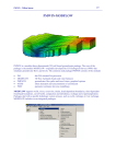
mesh used for the fluid domain of the simulation is shown in Figure 35.
Figure 35. The Eulerian mesh defining the fluid domain. The left image shows the shaded mesh. The right image
shows the Eulerian mesh drawn in wire frame with the Lagrangian elements of the tubing shaded.
During the development of the finite element model, a number of Eulerian mesh sizes and
shapes were experimented with. Initially a simple cubic domain with rectangular faces that
encompassed the entire fuel tank was used. This model resulted in a large number of elements
outside the tank walls which fluid could not flow into. The mesh shown in Figure 35 was found to
be a more efficient use of elements. Also shown in Figure 35, the Eulerian element size was
optimized so that finer elements were located in the region encompassing the tubing, and more
coarse element sizes were used elsewhere.
Abaqus Explicit provides the ability to have the Eulerian mesh track the motion of surfaces on
the Lagrangian mesh. The benefit of this feature is that it reduces the number of elements
required to define the fluid domain. The tracking surface used in the analysis was defined by the
elements of the fuel tank walls.
44
Initial Fluid Position
For this research study the initial conditions were such that the draw/return tubing is partially
immersed in fluid. A condition required by Abaqus Explicit is that the Eulerian material and the
Lagrangian material does not occupy the same three-dimensional space. To define the initial
position of the fluid, a utility was used from the Abaqus CAE pre-processing module, called the
Volume Fraction Tool. By default, all Eulerian elements in an Abaqus analysis are empty. An
element can be defined at the beginning of an analysis to be completely filled or partially filled
with material. An element variable called the “Volume Fraction” is used to denote the amount of
material within the element. For example, a value of 1.0 means completely filled, 0.5 is half
filled, and 0.0 is an empty element. The Volume Fraction Tool uses a reference, such as a 3D
CAD model, to define the enclosed volume of the fluid. As shown in Figure 36, an enclosed
surface volume was created which defined the initial fluid depth and accounted for the tubing
submerged below the surface of the fluid. A 0.5 mm offset was included to ensure the Eulerian
surface was not interfering with the Lagrangian elements.
Figure 36. In the image on the left, the Volume Fraction reference geometry is shown within the Eulerian element
domain. In the right-hand image, the resulting initial fluid position created by using the Volume Fraction Tool is shown
in cross section to highlight the clearance around the submerged tubing.
Contact and Fluid Structure Interaction
The interface between the fluid and structure was defined using the General Contact capability
of Abaqus Explicit. This formulation tracks free surfaces of the Eulerian fluid and the surfaces of
the Lagrangian components and enforces contact where they meet. The contact formulation
takes into account the thickness defined for the shell elements.
45
Material Definitions
Although the fuel tank and draw/return tubing were made from different aluminum alloys (5052
and 6061, respectively), a single generic set of aluminum material properties was use in this
analysis for convenience. Linear elastic properties were used to define the Lagrangian elements
since loading and the resulting strain in the parts was expected to be low, negating the need to
define plasticity. Material damping for the aluminum used the Rayleigh damping model, which
includes mass proportional (Alpha) damping and stiffness proportional (Beta) damping
parameters. These damping parameters were determined by performing an impulse response
test on the actual physical parts and then adjusting the parameters so that the simulation
matched the physical measured response. The aluminum material properties used for the
simulation are shown in Table 5.
Table 5. Aluminum Material Properties used in the simulation.
Density (ρ)
2.77E-9 tonne/mm
Modulus of Elasticity (E)
69000 MPa
Poisson’s Ratio (ν)
0.33
Mass Proportional
Damping (α)
4.8 s
Stiffness Proportional
Damping (β)
1.3E-7 s
3
-1
The material definition for the fluid used the linear Us-Up Equation of State (EOS) material model
that is provided within Abaqus Explicit. The Us-Up EOS relates the shock velocity (Us) to the
particle velocity (Up) through the linear expression Us = c0 + s Up, where c0 is the wave speed at
reference density and s is the Hugoniot slope. With the exception of fluid density, which had
been measured prior to testing, the required parameters to define the Us-Up EOS were taken
from an example problem included in the Abaqus Explicit documentation12. That example
described the analysis of a water-filled container which had sufficient similarity to the present
research. Viscosity was not specified for the fluid, with the assumption that the test conditions
would be dominated by inertial loads and viscous effects would be low by comparison. The fluid
material properties used for the simulation are shown in Table 6.
12
Abaqus Example Problems Manual: Example 2.3.2. “Impact of a water-filled bottle”
46
Table 6. Fluid material properties for the linear Us-Up Equation of State used in the simulation.
Density
1.003E-9 tonne/mm
wave speed (c0)
1.6E+6 mm/s
linear Hugoniot slope (s)
1.92
Grüneisen parameter (Γ)
0
3
Boundary Conditions and Loading
The position of the fuel tank was constrained using a kinematic coupling from a “master” node to
a group of “slave” nodes located on the bottom of the tank, shown in Figure 37. The masterslave connection serves as a representation of the tank’s constraints on the test fixture, and as
the input from the connecting rod. To constrain the motion of the tank to match the test fixture,
all rotational degrees of freedom and the vertical (Z-direction) and fore-aft (X-direction) degrees
of this master node were fixed.
Figure 37. A kinematic connection is defined from the master node (red triangle) to the slave nodes (yellow). Rotation
and translation constraints are defined at the master node.
47
The remaining degree of freedom of the master node, in the lateral (Y) direction, was set as an
enforced displacement from the time history data taken from the test fixture. This test data was
processed to filter out high-frequency noise and then converted to a tabular format called an
“Amplitude” definition in Abaqus.
Gravitational acceleration of 9810 mm/s2 (1 g) was applied at the beginning of the analysis step,
as a distributed load. Due to the relatively shallow depth of the fluid being studied, an initial
hydrostatic pressure in the fluid was not specified. During a short time period at the beginning of
the simulation, the influence of the applied gravity load caused the fluid to settle and wet the
surfaces of the tank and tubing.
Output
Output of results from the simulation model were requested as the solution progressed. These
included strain in the aluminum components, displacements, velocity, contact pressures
between the fluid and aluminum components, and the Volume Fraction of fluid in the Eulerian
elements. The rate of output requested was 200 records per second; a typical event simulation
lasting four seconds resulted in a total of 800 records. Additional output was requested at the
strain gage locations at a rate of 2 kHz for comparison with the test data collection rate which
had been recorded at a similarly high sample rate.
Computational and Other Considerations
Both Eulerian and Lagrangian meshes were created using the HyperMesh pre-processor, and
results review and plotting was completed using the HyperView post-processor. The total
number of Lagrangian elements used was 2960 and the total number of Eulerian elements were
93400. For this particular analysis model, the solver code for coupled Eulerian-Lagrangian
analysis in Abaqus Explicit was found to scale well using parallel execution on multiple
processors. A computational cluster was used to run the analysis solution, using Compute
Nodes connected with high speed network interfaces. A typical simulation utilized 36 processors
rated at 2.4 GHz, which were distributed across three Compute Nodes with 12 processors per
Compute Node. The input files were relatively small in size, totaling less than 17 MB. During
solution runtime the memory usage was less than 4 GB. The total run time to simulate an event
lasting four seconds typically required 28 hours (36 processors x 28 hours = 1004 processor
hours). The output data result file size of a four-second simulation event was 6.3 GB.
48
Chapter 6: Results
Two test events were run on the oscillation test fixture. The displacement data collected from
both events was processed to extract a time history of each event. The displacement history
from the test was used as the input to produce an equivalent simulation event to match the test.
Video data was collected during the test event and was converted to surface scan data with the
Slosh-Test software. Both of the events were repeated multiple times and the collected data
from the repeated runs were compared to ensure a consistent set of data.
Event Descriptions
The first event, named Event005, was a periodic oscillation with a relatively smooth start and
stop. The period of oscillation was established by setting the electric motor speed to 1400 RPM,
giving an approximate oscillation period of 1.7 seconds ( 0.58 Hz). The electronic timer was set
to activate the electromagnetic clutch for 3.4 seconds producing a total of two strokes of the
shuttle and tank returning it to the original starting point, after which the brake was applied to
stop the movement of the tank and hold it in a stationary position. The start/stop position for the
test is shown in Figure 38.
Figure 38. The start/stop position for Event005. The crank disc rotated clockwise for a total of two full revolutions.
The second event, named Event008, was a half-sinusoidal oscillation with very abrupt start and
stop. The period of oscillation was established by setting the electric motor speed to 1200 RPM
resulting in an oscillation period of 2 seconds (0.5 Hz). The electronic timer was set to activate
the electromagnetic clutch for 1 second, followed by application of the brake. As shown in
Figure 39, the initial starting position of the shuttle placed it in the middle of the oscillation cycle.
49
As a result, when the clutch was activated the shuttle rapidly accelerated. Likewise the stop
position when the brake was applied, shown in Figure 39, occurred when the shuttle was at the
highest velocity on the return stroke of the oscillation, resulting a rapid deceleration.
Figure 39. The start/stop positions for Event008, shown in the left and right images, respectively. The crank disc
rotation was clockwise.
Displacement and Acceleration Time History
The following figures show the displacement and acceleration of the two events. The measured
data from the motion of the shuttle on the test fixture is reflected in the displacement plots
(Figures 40 and 42) and came as a result of the response of the simulations. The acceleration
plots are a derived result from the simulation’s displacement response (Figures 41 and 43).
Figure 40. The displacement time history for Event005. The data source is from the simulation output.
50
Figure 41. The acceleration time history for Event005. The acceleration signal is derived from the displacement time
history by twice differentiating it with respect to time and then applying a low-pass Butterworth filter to remove highfrequency content.
Figure 42. The displacement time history for Event008. The data source is from the simulation output.
51
Figure 43. The acceleration time history for Event008. The acceleration signal is derived from the displacement time
history by twice differentiating it with respect to time and then applying a low-pass Butterworth filter to remove highfrequency content.
Force Transducer Time History and Spectral Analysis
The following figures show the measured force data from the axial transducer on the test fixture
in both time history and spectral analysis. When creating the spectral analysis graphs, the time
signal was divided into two sections for processing. The first section was the time during the test
when the shuttle was moving and the second section was when the shuttle was held stationary.
The spectral analysis used a fast Fourier transform (FFT) algorithm, with buffer size of 1024
samples and a 67% buffer overlap.
52
Figure 44. The force transducer output for Event005. A low-pass Butterworth filter was used to remove frequency
content above 50 Hz.
Figure 45. The power spectral density (PSD) of the force transducer data from Event005. The time signal was
processed in two segments The red line is when the shuttle is actively being moved at the beginning of the test event.
The blue line is when the shuttle was being held stationary by the brake. Vertical axis units are Newton squared
2
divided by Hz (N /Hz), and the horizontal axis units are Hz. The PSD was generated using unfiltered data.
53
Figure 46. The force transducer output for Event008. A low-pass Butterworth filter was used to remove frequency
content above 50 Hz.
Figure 47. The power spectral density (PSD) of the force transducer data from Event008. The time signal was
processed in two segments The red line is when the shuttle is actively being moved at the beginning of the test event.
The blue line is when the shuttle was being held stationary by the brake. Vertical axis units are Newton squared
2
divided by Hz (N /Hz), and the horizontal axis units are Hz. The PSD was generated using unfiltered data.
54
Strain Time History and Spectral Analysis
The following figures show the strain time history and spectral analysis for the test and
simulation of both events. The complete time signal was processed for the spectral analysis
using an FFT algorithm with buffer size of 1024 samples and a 67% buffer overlap.
Figure 48. The strain time history at gage #3 on the test fixture (red line, top) and element #3 of the simulation (blue
line, bottom) for Event005. Vertical axis units are microstrain (με) and the horizontal axis units are seconds. A lowpass Butterworth filter was used to remove high-frequency content above 50 Hz.
55
Figure 49. The strain time history at gage #3 (red) and element #3 (blue) for Event005 overlaid on a single graph.
Vertical axis units are microstrain (με) and the horizontal axis units are seconds. A low-pass Butterworth filter was
used to remove high-frequency content above 50 Hz.
Figure 50. The power spectral density (PSD) of gage #3 on the test fixture (red) and element #3 (blue) of the
2
simulation for Event005. Vertical axis units are microstrain squared divided by Hz (με /Hz) and the horizontal axis
units are Hz. The PSD was generated using unfiltered data.
56
Figure 51. The strain time history at gage #3 on the test fixture (red line, top) and element #3 of the simulation (blue
line, bottom) for Event008. Vertical axis units are microstrain (με) and the horizontal axis units are seconds. A lowpass Butterworth filter was used to remove high-frequency content above 50 Hz.
Figure 52. The strain time history at gage #3 (red) and element #3 (blue) for Event008 overlaid on a single graph.
Vertical axis units are microstrain (με) and the horizontal axis units are seconds. A low-pass Butterworth filter was
used to remove high-frequency content above 50 Hz.
57
Figure 53. The power spectral density (PSD) of gage #3 on the test fixture (red) and element #3 (blue) of the
2
simulation for Event008. Vertical axis units are microstrain squared divided by Hz (με /Hz) and the horizontal axis
units are Hz. The PSD was generated using unfiltered data.
Free Surface Fluid Motion
The following figures show the fluid’s free surface conditions for the test and simulation. The
images in each figure are grouped together showing separate test and simulation results as well
as an overlay at each point in time. For brevity only a small set of time points are represented in
the figures, and the complete event is not shown (truncated at approximately time t = 2.5
seconds).
58
Figure 54. The free surface of the fluid from test scan and simulation for Event005 at times (top to bottom) 0.06
seconds, 0.33 seconds, and 0.60 seconds. Shown left to right are the overlay of both results, the scanned result, and
simulation result, respectively.
59
Figure 55. The free surface of the fluid from test scan and simulation for Event005 at times (top to bottom) 0.85
seconds, 1.16 seconds, and 1.43 seconds. Shown left to right are the overlay of both results, the scanned result, and
simulation result, respectively.
60
Figure 56. The free surface of the fluid from test scan and simulation for Event005 at times (top to bottom) 1.69
seconds, 1.96 seconds, and 2.25 seconds. Shown left to right are the overlay of both results, the scanned result, and
simulation result, respectively.
61
Figure 57. The free surface of the fluid from test scan and simulation for Event008 at times (top to bottom) 0.00
seconds, 0.26 seconds, and 0.52 seconds. Shown left to right are the overlay of both results, the scanned result, and
simulation result, respectively.
62
Figure 58. The free surface of the fluid from test scan and simulation for Event008 at times (top to bottom) 0.78
seconds, 1.05 seconds, and 1.31 seconds. Shown left to right are the overlay of both results, the scanned result, and
simulation result, respectively.
63
Figure 59. The free surface of the fluid from test scan and simulation for Event008 at times (top to bottom)
1.57seconds, 2.12 seconds, and 2.38 seconds. Shown left to right are the overlay of both results, the scanned result,
and simulation result, respectively.
64
Chapter 7: Discussion
Displacement and Acceleration
The displacement time history from the simulation of Event005 (Figure 40) shows a sinusoidal
response with the expected displacement profile that was observed on the test fixture for the
corresponding event. As anticipated, the peak accelerations shown in Figure 41 had relatively
low magnitude in the range of +/- 0.6 g. The acceleration signal had notable high and lowfrequency components.
The displacement time history from the simulation for Event008 (Figure 42) showed a halfsinusoidal response, as expected. The peak accelerations were in the range of +1.0 g to -1.6 g
with notable ringing in the signal at the start and stop points of the shuttle motion, which was
expected based on the “hard” start and stop nature of the event.
Input Force from the Electromechanical Drive
The input force for both events measured on the test fixture had evidence of high-frequency
pulsation that can be seen in Figure 44 (Event005) and Figure 46 (Event008). The pulsation
was observed when the mechanical drive was actively moving the shuttle. The spectral analysis
of the force data, in Figure 45 (Event005) and Figure 47 (Event008), show a dominant
frequency peak at 23 Hz for the active movement portion of the force time history. This
dominant peak was almost non-existent for the portion of the signal when the shuttle was held
stationary at the end of the test events. The transition period from active to stationary is shown
in Figure 60 (Event005).
65
Figure 60. The force transducer output for Event005 is shown for the 2 –5 second time period . At 3.4 seconds, the
electric motor was disengaged and the brake was applied. Two filter settings were used to process the data using a
low-pass Butterworth filter. The red line is from a 50 Hz cut-off filter; the blue line is from an 8 Hz cut-off filter.
In Figure 60, the time period from 2 seconds to 3.4 seconds shows the active portion during the
event when the electromagnetic clutch was engaged. The force during this time period is a
combination of the load that was required to accelerate and decelerate the shuttle and tank, as
well as the load required to react the sloshing of the fluid inside the tank. At 3.4 seconds, the
clutch was disengaged and the brake was applied. From 3.4 seconds through the remainder of
the force time history signal, the force value shown in Figure 60 is a result of only the load from
the sloshing fluid.
While some pulsation is expected from a mechanical drive system, the amplitude and frequency
of the pulsation observed was particularly undesirable.
The low-frequency content of the force input, the blue line in Figure 60, had a range of +/- 280
Newtons. The pulsation amplitude, the red line in Figure 60, was in a range of +/- 80 Newtons.
This represented an excessive amount of “noise” compared to the “signal.”
66
A normal modes analysis was performed using a finite element model of the draw/return tube
assembly (Appendix D). The analysis in Appendix D shows that the lowest natural frequency of
vibration was at 26 Hz, and the mode shape was a lateral bending of the tubes. During testing,
this natural vibration at 26 Hz was confirmed on the actual draw/return assembly by reviewing
the strain response during events that were performed with an empty tank. When fluid was
added to the tank, this vibration shifted to a lower frequency range of 19 to 21 Hz.
With the relatively high amplitude and a pulsation frequency near the natural vibration of the
draw/return tubing, there is a strong likelihood that this undesirable pulsation resulted in
excitation of the tubing and increased the strain levels at the gage locations. An investigation
was made to identify the source of the pulsation in the electromechanical drive system, and the
details of that investigation are included as Appendix C. The findings of that investigation
indicate that the pulsation coincides with the rotational frequency of the electric motor.
There was insufficient time to make the required modifications to address this force pulsation
issue during this research project. A suggested change that could reduce the amplitude of
pulsation would be to replace the electric motor with one having a higher torque rating.
Additionally, an in-line axial damper or bushing could be installed. Alternatively, changing to a
higher speed motor and to a gearbox with increased gear reduction could shift the pulsation to a
higher frequency which would be less likely to excite a resonant response in the tubing.
Strain response
Generally, there was a poor correlation between the strain data of the lab tests and the strain
response in the simulations. Below, the data from the test is presented first for each event,
followed by a discussion of how well the simulation matched the test.
In Event005, the strain gage signal response from the test was relatively smooth, with evidence
of resonance and damping. The amplitude of vibration in the strain signal grew and subsided as
the fluid flowed past the tubing and as the tank oscillation accelerated and decelerated. The
frequency content of the test signal shows a dominant peak at 22 Hz. A minor peak is present at
60 Hz, which is most likely due to electrical noise from the main power line frequency.
In contrast, the simulation strain response for Event005 shows a significant amount of noise
compared to the test data. When viewed separately (Figure 48), the two strain signals appeared
67
to have almost no correlation. When the test and simulation data were overlaid on the same plot
(Figure 49), a general trend of rising and falling strain levels could be seen, although the
correlation was minor. The simulation data, as seen in the power spectral density plot (Figure
50), shows a broad range of frequency content from 10 Hz to 30 Hz, with two peaks within that
range. The first was a minor peak at 22 Hz, and then a dominant peak at 26 Hz. The minor peak
at 22 Hz correlates with the same frequency value of the dominant peak in the test data.
However, there was no correlation with the dominant 26 Hz peak of the simulation with the test
data.
There was also a significant discrepancy in the strain gage amplitude between the test and
simulation for Event005 shown in Table 7. The simulation was found to overpredict the strain
amplitude by a factor of three.
Table 7. Event005 strain gage amplitude details from the test and simulation. Units are microstrain (με).
Max
Min
Max Range
(peak-to-peak)
Test
55
-73
110
Simulation
178
-189
360
In Figure 51 (Event008) the strain gage signal of the test data had a sharp initial rise as was
expected from the sudden acceleration of the event. After an initial peak in strain amplitude near
the beginning of the event, the vibration in the strain gage signal appears to damp until a
sudden deceleration occurs when the test fixture brake was applied at roughly 1.1 seconds. The
remaining portion of the data signal showed progressive damping with small periodic mean
oscillation which likely came from the residual fluid motion. The frequency content (Figure 53) of
the test data had a dominant peak at 22 Hz with a minor peak at 60 Hz, which was similar to
that of Event005.
With the test and simulation strain signals of Event008 overlaid on a single plot (Figure 52),
there is a common general trend apparent with the two signals. At the beginning of the test, both
strain levels quickly increased and reached a maximum amplitude. The two data sources
correlate well with both the strain magnitude and sign (compressive strain). The two signals
then diverge, with the simulation shrinking in amplitude much more rapidly and in a manner that
does not appear to be a damped response. The simulation strain signal then grows in amplitude
68
and contracts and repeats this behavior though the remainder of the event. The growth and
contraction in strain amplitude of the simulation signal did not appear to be a regular periodic
interval. In Figure 52, at time t = 1.1 seconds when the brake was applied, the simulation strain
signal again correlated fairly well with the correct compressive strain, although it overpredicted
the magnitude by roughly 70 percent. The frequency content of the simulation strain signal in
Event008 (Figure 53) showed a dominant peak at 19 Hz, and a minor peak at 42 Hz.
The strain amplitude comparison for the simulation and test is shown in Table 8.
Table 8. Event008 strain amplitude details for the test and simulation. Units are microstrain (με).
Max
Min
Max Range
(peak-to-peak)
Test
180
-180
360
Simulation
144
-234
325
An examination of the simulation results was done in an attempt to find the source of noise in
the strain signal. The fluid-to-structure interface was found to be very active with the creation of
cavities. These void-filled pockets were generally small and were found to form and collapse at
the structure’s surface, both at the tank walls and on the tubing. Since the simulation model did
not include air or atmospheric pressure, these cavities collapsed relatively slowly by just the
influence of gravity and local fluid motion. Occasionally there were large “bursts,” as shown in
Figure 61, where very large cavities were formed. These large and small bursts were found to
correspond with elevated strain response in the gage elements, and are thought to be the likely
source of noise.
69
Figure 61. A cross section of the tank (left) showing detail (right) at the fluid-tubing interface. The contours are
velocity magnitude for the fluid, in millimeters per second. From top to bottom, the series of images show the creation
of a cavity as the fluid “bursts” outward from the submerged tubing. Each frame represents 80 milliseconds.
70
Free Surface Fluid Motion
The simulation and test results for fluid motion were found to match very well. Upon reviewing
the animated results, which are depicted in the time-lapse images of Figures 54 through 59, the
speed and height of the waves moving through the fluid had good correlation between the test
and simulation. This close correlation was found to be evident in both of the test events.
Some limitations of the scanning system are evident when reviewing the results of the test and
simulation side-by-side. During periods of relatively smooth motion, the scanning system was
able to track and record a majority of the fluid surface definition. When there was a significant
amount of splash and spray inside the tank, the scanning system had difficulty processing the
chaos. An example is shown in Figure 62. At these points in time, large areas of the fluid
surface were seen to be undefined, and the areas that did have definition contained a large
amount of obvious error.
Figure 62. A particularly difficult point in time for the surface scanning system is shown from Event008 at time t =
1.57 seconds. The simulation in the lower left shows conditions inside the tank, with a large amount of noncontiguous fluid. The two images in the top row are the camera views from the test fixture at the same time point. The
lower right image is the resulting scanned surface from the two top images.
71
The primary difficulty of the scanning system was a combination of non-contiguous fluid
blocking the laser illumination from above (free-flying fluid “blobs” and droplets), and from fluid
splashed on the transparent cover. To reduce the effect of fluid splash on the acrylic cover,
which blocked and distorted the camera’s view, the inside of the cover had been treated with a
wax coating. For the two events run for this research study, the periods of time where the
scanning system was not capable of representing a sufficient surface definition were brief. Once
the cover had shed most of the fluid droplets and splashing had subsided the scanning system
returned to producing favorable results.
72
Chapter 8: Conclusion
The study was successful in meeting most of the objectives established for the project. The
following summary reviews individual objectives and how well they were met along with possible
improvements for future research work.
A test fixture was designed and constructed with automated features that enabled several
events to be run with varying parameters. The automation that was included, particularly the
digital timer and electromagnetic clutch/brake unit, allowed for a single event to be repeated to
build confidence in the data that was collected. The variable speed motor and adjustable stroke
length settings of the crank disc made it possible to tune the sloshing of the fluid to desired level
with ease. An issue that needs to be addressed is to reduce the pulsation created by the input
force transmitted from the electromechanical drive train. This pulsation occurred in the
frequency range of the tube assembly's natural resonance, leading to a concern that the strain
response in the tubing may be due in part to the test fixture and not entirely from the fluid
motion. Some potential changes to the test fixture would be to replace the electric motor with
one with a higher speed rating coupled to a gear reducer with increased reduction ratio.
Alternatively, substituting the motor with one at the same speed rating but with a higher torque
and output power rating could also result in lower amplitude of pulsation. An addition of an inline axial mechanical damper on the push rod could also be investigated.
The fluid scanning system that was developed was successful in capturing the motion of the
fluid sloshing within the tank. While the system was found to have some limitations, overall it
exceeded expectations for the project. The use of alternating color for the laser illumination
proved to be beneficial in identification of the individual laser lines. It is possible that the
scanning system could be further improved by the inclusion of a third color (such as 530 nm
green lasers). Additional improvements are also possible within the scanning software that was
developed, particularly the line processing and identification algorithm. Optimization for
performance and an increase in correctness of laser line identification are likely to result from
further development of the scanning software code.
73
The coupled Eulerian-Lagrangian analysis simulation model that was developed to recreate the
test conditions was only partially successful. The motion of the of the fluid in the simulation was
found to correlate fairly well with that of the test. However, the strain in the tubing was found to
have poor correlation to the data collected on the test, both in total strain amplitude and in
frequency content. A potential change to the model which could improve the correlation with test
would be to decrease the element size used in either the Eulerian fluid mesh, the Lagrangian
structure mesh, or both. This could improve the fluid and structure contact interface which may
reduce the amount of “bursts” of pressure that were found to occur. However, decreasing
element size would result in increased computational costs, both in hardware and commercial
software licensing that would be required to complete the simulation within a reasonable time
frame.
As a final comment, the overall goal of the research project was met, in that a much deeper
understanding of the conditions that exist when fluid sloshes within a cylindrical fuel tank was
achieved.
74
Acknowledgements
Completing this research was a significant task that would not have been possible without the
help and support that I received along the way. I would like to thank Per Reinhall for his
guidance and Jim Riley, Alberto Aliseda, and Mark Van Sickle for their feedback and
encouragement. I would like to thank Dana Dabiri for providing a wealth of reference material for
research. I would like to thank the staff at the Kenworth Research and Development Lab for
providing me with parts for assembly: Don Williams for fabricated sheet metal parts; Duane
Rawls for milling; Walt Benz for fabrication and welding; and Larry Gulan for his consultation on
the initial design of the test fixture. I would like to thank Bob Gillett for support on electrical
wiring, Lena Kartzov for providing artwork, and Jennifer Knutson for technical editing. I want to
express appreciation to my supervisor, Rick Drollinger, for providing the accommodation to
make this project fit into our busy work schedule. I would like to thank my colleagues at
Kenworth Division and at the PACCAR Technical Center for helping me brainstorm and for
sharing their wealth of knowledge. I would like to give a special “thank you!” to my wife, AnnMarie, whose love, understanding, and support were invaluable. And finally, a huge thanks to
my daughter Alena for her patience.
75
References
Abaqus Analysis User’s Manual (6.12). Chapter 6.3.3 Explicit dynamic analysis.
Abaqus Example Problems Manual (6.12). Example 2.3.2. “Impact of a water-filled bottle”.
Bakhsi, A. S., and D. E. Smith. "Effect of Fat Content and Temperature on Viscosity in Relation
to Pumping Requirements of Fluid Milk Products." Journal of Dairy Science 67 (1984).
Bateman A, Granados A, Medina V, Nalesso M, Velasco D (2006) Experimental procedure to
obtain 2D time-space high-speed water surface. In: Ferreira R, Alves E, Leal J, Cardoso
A (eds) River flow 2006. Taylor & Francis, London, pp 1879–1888
"Calib3d. Camera Calibration and 3D Reconstruction." Camera Calibration and 3D
Reconstruction — OpenCV 2.4.5.0 documentation. 13 June 2013
<http://docs.opencv.org/modules/calib3d/doc/calib3d.html>.
"Density." Wikipedia. 06 June 2013. Wikimedia Foundation. 12 June 2013
<http://en.wikipedia.org/wiki/Density>.
"Homogeneous coordinates." Wikipedia. 30 May 2013. Wikimedia Foundation. 13 June 2013
<http://en.wikipedia.org/wiki/Homogeneous_coordinates>.
"Lee presents Viscosity of various fluids." Lee presents Viscosity of various fluids. 13 June 2013
<http://www.microhydraulics.com/LEEWEB2.NSF/1c6397740f8b45e1852563b9006d6bc6
/4fb2037fc902397a8525689b00654b3a!OpenDocument>.
"Viscosity." Wikipedia. 06 Oct. 2013. Wikimedia Foundation. 13 June 2013
<http://en.wikipedia.org/wiki/Viscosity>.
76
Appendix A: Strain Gage Installation on Draw/Return Tubing
The following images show the strain gage locations and specific details of the gages used.
Small Tube
Gages 1 & 2
CEA-13-250UN-350
Gage Factor:
2.13 + .5%
Kt =
(0.3 + .2)%
Adhesive:
AE-10
Large Tube
Gages 3 & 4
CEA-13-250UN-350
Gage Factor:
2.13 + .5%
Kt =
(0.3 + .2)%
Adhesive:
AE-10
77
78
Appendix B: Laser Module Alignment and Wiring Diagram
Alignment
The laser alignment was performed by placing a sheet of pre printed graph paper on to the
lower surface of the tank and using it as guide. The paper was indexed from the inside surface
of the acrylic cover and taped in place. Then the lasers, which were installed loosely in the
machined aluminum mounting block, were rotated to be parallel with the transparent cover. To
set this parallel alignment, the outer ends of the laser line, where it ran off the edge of the grid
paper, were placed on a common grid value. At this point, the outer ends of the laser line were
now on a common grid value, but the laser line position at the bottom-center of the tank was
typically offset either forward or backward. This indicated the plane of the laser line had a slope
from top to bottom. Further adjustment was done using shims on the laser modules to bring
them into closer agreement with the outer end values. Three measurement values were
recorded in a spreadsheet and then averaged yielding a single value. When the alignment
process was completed the set screws holding the laser modules were tightened and secured
with a small drop of hot melt adhesive. Figure B1 to B6 show some of the steps in the alignment
process. Table B1 shows the results of the alignment that was used for testing in this study. The
averaged value is used as input to the scanning software, and represents depth (“Z” in camera
coordinates) when performing the perspective transformation.
Figure B1. Before alignment. A flat board installed
inside the tank was used help set the focus on the
laser lenses.
Figure B2. Graph paper with preprinted increments.
Brown line spacing: 50 mm. Black triangle pattern size:
10 mm. Black triangle pattern line spacing: 2 mm.
79
Figure B3. Red laser lines are in the process of having
the outer left edge set.
Figure B5. Alignment complete.
Figure B4. Red laser lines are in the process of being
adjusted at the center.
Figure B6. Laser modules with set screws and small
drop of hot melt adhesive.
Table B1. The measurements of laser alignment. The distance is from the inside surface of the transparent acrylic
cover, with units of millimeters. Measurements were done at three locations then averaged.
Line #
Left Edge
Middle
Right Edge
Average
1
45.5
46.5
45.5
45.8
2
80
79
78.5
79.2
3
116
115
116
115.7
4
150
149
149.5
149.5
5
190.5
191
190.5
190.7
6
223
222
224
223.0
7
262
261.5
262
261.8
8
294.5
293.5
295.5
294.5
80
9
335.5
335
335.5
335.3
10
377
378
377
377.3
11
410
410.5
411.5
410.7
12
446
446.5
448
446.8
13
487
488.5
490.5
488.7
14
519
518
522
519.7
Laser Module Circuit Diagram
The electrical circuit diagram for the laser system is shown below in Figure B7.
Figure B7. Laser control panel switches (left image) and the laser module circuit diagram (right image).
81
Appendix C: Investigation of Excessive Vibration in the
Electromechanical Drive System
A study was conducted to find the source of excessive pulsation that had been observed in the
mechanical drive system. To assess the response of the pulsation with varying amounts of
mass, the oscillation test fixture was run at several fluid levels. While the fluid level was varied,
a constant motor speed was used. Figures D1 through D3 show data that was collected for
three fill levels.
Figure C1. The power spectral density plot for a test event with the motor speed set to 1240 RPM and with no fluid in
the tank. The data lines represent the displacement (red), force (blue) and gage 3 strain (green) data from the test.
82
Figure C2. The power spectral density plot for a test event with the motor speed set to 1240 RPM and with 24 liters
of fluid in the tank. The data lines represent the displacement (red), force (blue) and gage 3 strain (green) data from
the test.
83
Figure C3. The power spectral density plot for a test event with the motor speed set to 1240 RPM and with 42 liters
of fluid in the tank. The data lines represent the displacement (red), force (blue) and gage 3 strain (green) data from
the test.
With the fuel tank empty the dominant frequency of the gage 3 strain signal was 28 Hz (Figure
C1), which closely correlates with the first natural frequency of the draw/return tube assembly,
which was 26 Hz. The dominant frequency of the force signal was 19 Hz. When 24 liters of fluid
were added to the tank, the dominant frequency of the gage 3 strain signal shifted down to 21
Hz (Figure C2). When the fluid quantity was increased to 42 liters (Figure C3) the dominant
frequency of the gage 3 strain signal shifted down to 20 Hz. The dominant frequency of the
force signal remained roughly unchanged, at 19 Hz, as fluid was added to the tank. This
indicated that the force pulsation frequency was minimally affected by an increase of inertial
loading.
The oscillation test fixture was run at several electric motor speeds to evaluate the effect on the
force pulsation. Figures D4 through D7 show the power spectral density plots for four different
electric motor speed settings.
84
Figure C4. The power spectral density plot for the fixture running with the electric motor speed set to 400 RPM, with
no fluid in the tank. The data for displacement (red), force (blue), gage 3 strain (green), and acceleration (pink) are
shown.
Figure C5. The power spectral density plot for the fixture running with the electric motor speed set to 800 RPM, with
no fluid in the tank. The data for displacement (red), force (blue), gage 3 strain (green), and acceleration (pink) are
shown.
85
Figure C6. The power spectral density plot for the fixture running with the electric motor speed set to 1260 RPM, with
no fluid in the tank. The data for displacement (red), force (blue), gage 3 strain (green), and acceleration (pink) are
shown.
Figure C7. The power spectral density plot for the fixture running with the electric motor speed set to 1700 RPM, with
no fluid in the tank. The data for displacement (red), force (blue), gage 3 strain (green), and acceleration (pink) are
shown.
When the motor speed setting was 400 RPM, shown in Figure C4, there was no apparent
dominant peak in the force signal. When the motor speed was increased to 800 RPM (13
86
rev/sec), shown in Figure C5, a dominant peak in the force signal at 13.6 Hz became evident.
With increase of motor speed to 1260 RPM (21 rev/sec) and 1700 RPM (28.3 rev/sec), shown in
Figures C6 and C7 respectively, the dominant peak in the force signal increases to 19.5 Hz and
29.3 Hz, respectively. The response shown in Figures C4 through C7 indicates a strong
correlation between the input force pulsation and the electric motor speed.
87
Appendix D: Normal Modes Analysis
A normal modes analysis was performed on the fuel tank and draw/return tubing to identify the
natural resonant frequencies that could become excited. The tank was constrained at the two
ends of the cylindrical section. There was no inclusion of fluid. The first two modes of vibration
are shown in Figure D1 and D2.
Figure D1. First mode of vibration at 26 Hz. The green outline represents the undeformed state. The blue and yellow
draw/return tubes are bending laterally across the axis of the fuel tank.
88
Figure D2. Second mode of vibration at 43 Hz. The green outline represents the undeformed state. The blue and
yellow draw/return tubes are bending fore-aft along the cylindrical axis of the fuel tank.
89