1
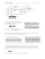
1/37 PMWIN – Willem Spaans _____________________________________________________________________________________________________ PMWIN-MODFLOW PMWIN is a modular three-dimensional (3D) cell based groundwater package. The core of the package is the module MODFLOW –originally developed by US Geological Survey (1988)- that simulates groundwater flows and levels. The common used package PMWIN consists of the modules • • • • • PM MODFLOW PMPATH MT3D PEST the GIS oriented Pre-processor 3D flow, hydraulic heads and water balances groundwater flow paths and travel times, graphical options solute transport and concentrations of constituents parameter estimator (inverse modelling) MODFLOW supports wells, rivers, reservoirs, drains, head-dependent boundaries, time-dependent fixed-head boundaries, cut-off walls, compaction and subsidence, recharge and evapotranspiration. Packages deal with a specific hydrologic system stresses, such as wells, recharge or river exchange. MODFLOW includes seven integrated packages: 2/37 PMWIN – Willem Spaans _____________________________________________________________________________________________________ The various PMWIN modules are ‘stand- alone’ and communicate through data files. Package 1. Drain 2. River 3. Well 4. Evapotranspiration 5. General head boundary 6. Time-Variant Specified-Head 7. Reservoir 8. Wetting capability 9. Horizontal-Flow Barrier 10. Interbed-Storage 11. Density 12 Stream flow-Routing Feature Simulates only inflow into a drain with fixed level and drain resistance (leakance) Simulates inflow and outflow from a river with fixed level and bottom resistance (leakance) Simulates the effect of abstraction or recharge of a layer penetrating well with fixed flow rate Simulates the abstraction from the upper aquifer from a user defined evapotranspiration rate Simulated the flow from a cell with a fixed head in relation to the computed groundwater table. Allows constant-head cells to take on different values for each time step Simulates leakage between a reservoir and an underlying ground-water system as the reservoir area expands and contracts in response to changes in reservoir stage. Re-activates a dry cell when the water table in adjacent cells justify this Simulates thin, vertical low-permeability geologic features (such as cutoff walls) that impede the horizontal flow of ground water Simulates storage changes from both elastic and inelastic compaction in compressible fine-grained beds due to removal of groundwater. Simulates the effect of density differences on the groundwater flow system. Accounts for the amount of flow in streams and to simulate the interaction between surface streams and groundwater More info on manuals and software can be found at http://www.ihw.ethz.ch/publications/software/pmwin/index_EN The module PMPATH uses a semi-analytical particle-tracking scheme to calculate the three dimensional path lines and location of particles in time and space at user defined time levels. At these time levels the flow conditions are assumed to be steady state. Forward tracking allow for path and total travel time computations, backward tracking to determine the origin of sources or discharge points. Computation and display of path(flow)lines and travel time are done simultaneously, the various on-screen graphical options include head contours, drawdown contours and velocity vectors. The semi-analytical particle-tracking scheme is based on the assumption that each directional velocity component varies linearly within a grid cell, describing the pathline within a grid cell. The new position of a particle is computed from its ‘initial’ position anywhere in a cell. Note that dispersion, reactions and adsorption are included on top of the transport. The MT3D transport module simulates changes in concentration of single species miscible contaminants in groundwater considering advection, dispersion and simple chemical reaction. The flow simulation is done separately in Modflow, assuming that changes in the concentration field will not significantly affect the flow field. Concentration computations are based on the threedimensional advective-dispersive-reactive transport equation. The solution method can be the method of characteristics; using either the traditional MOC approach, a hybrid approach, or others. The concentrations of one single species are adjusted for advection, dispersion and some simple chemical reactions. The chemical reactions included in the model are limited to equilibrium-controlled linear or non-linear sorption and first-order irreversible decay or biodegradation. 3/37 PMWIN – Willem Spaans _____________________________________________________________________________________________________ MT3DMS is a multi-species development of MT3D and includes three major classes of transport solution techniques, i.e., the standard finite difference method; the particle tracking based EulerianLagrangian methods; and the higher-order finite-volume TVD method. Up to 30 different species can be simulated. In addition MT3DMS includes an implicit iterative solver based on generalized conjugate gradient (GCG) methods. If this solver is used, dispersion, sink/source, and reaction terms are solved implicitly without any stability constraints. The MOC3D transport model is based on the method of characteristics. It computes changes in concentration of a single dissolved chemical constituent over time that are caused by advective transport, hydrodynamic dispersion (including both mechanical dispersion and diffusion), mixing or dilution from fluid sources, and mathematically simple chemical reactions, including decay and linear sorption represented by a retardation factor. The transport equation is solved using the hydraulic gradients computed with MODFLOW for a given time step. The user can apply MOC3D to a sub grid of the original MODFLOW grid. However, the transport sub grid must have uniform grid spacing along rows and columns. PEST and UCODE assist in data interpretation and model calibration uses observation data for automatically calibration of model parameters: (1) horizontal hydraulic conductivity or transmissivity; (2) vertical leakance; (3) Specific yield or confined storage coefficient; (4) pumping rate of wells; (5) conductance of drain, river, stream or head-dependent cells; (6) recharge flux; (7) maximum evapotranspiration rate; and (8) inelastic storage factor. The model parameters and/or excitation data are adjusted such that the discrepancies between the pertinent model-generated numbers and the corresponding measurements are reduced to a minimum. The graphical user-interface allows creating and simulating models with an irregular rectangular grid, and can handle up to 1,000 stress periods, 80 layers and 250,000 cells in each model layer. Modelling tools include Presentation Result Extractor Field Interpolator Field Generator Water Budget Calculator Graph Viewer Allows for labelled contour maps of input data and simulation results. Report-quality graphics can be saved in file formats SURFER, DXF, HPGL and BMP Creates two dimensional animation sequences of calculated head, drawdown or concentration Extracts simulation results like hydraulic heads, drawdowns, cell-by-cell flow terms, Darcy velocities, concentrations and mass terms from any period to a spreadsheet. Results can be saved in ASCII or SURFER files Interpolates discrete measurement data to each model cell. The model grid can be irregularly spaced. Generates heterogeneously distributed transmissivity or hydraulic conductivity. It allows the user to statistically simulate effects and influences of unknown small-scale heterogeneities. Calculates the flows in and exchanges between layers at user defined zones It can show the flow through a particular boundary. Displays time curves of results including hydraulic heads, drawdowns, and concentrations. 4/37 PMWIN – Willem Spaans _____________________________________________________________________________________________________ Groundwater modelling using PMWIN The three dimensional space is considered as a sequence of layers, each having their specific properties in terms of top and bottom level, permeability, and storativity. The three dimensional space is discretized in terms of blocks formed by cells (∆x, ∆y) and layers. Hydraulic heads, internal flows and external hydrological stresses are defined in the centre of each block. The cell size in the same for all layers over the vertical, transmissivities are computed from the permeabilities and the water bearing part of the layers. Each cell or block can be defined as (1) free level or variable head, (2) fixed level or constant head, or (3) to be inactive. The latter allows irregular shaped domains. Flow conditions can be steady or unsteady (transient). The length of the simulation or total computation time can be subdivided in stress periods representing time intervals with constant hydrological conditions. Each stress period can be subdivided in a number of computation time steps ∆t. 5/37 PMWIN – Willem Spaans _____________________________________________________________________________________________________ For each time interval ∆t the mass balance is defined for each cell or block. This yields a set of simultaneous linear equations, which is solved using standard solution procedures. The resulting hydraulic heads and related flows provide a flow pattern in space and time. The same holds for the concentration computations using MT3D. From this flow patterns, pathlines and drawdowns can be computed accordingly. Storage components Storage terms are required for unsteady flow simulations Effective porosity is used for determination of the average velocity in the pore space or transport velocity, and is defined as the ratio flow void space/total volume. Effective porosity (with respect to flow through the medium) is normally smaller than porosity, because some fluid in the pore space is immobile. This may occur when the flow takes place in a fine- textured medium where adhesion (i.e., the attraction to the solid surface of the porous matrix by the fluid molecules adjacent to it) is important. Effective porosity is used by the transport modules PMPATH, MOC3D and MT3D/MT3DMS, to calculate the Storage terms are required for unsteady flow simulations of the flow through the porous medium. If a dual-porosity system is simulated by MT3DMS, effective porosity should be specified as the portion of total porosity filled with mobile water (Zheng and Bennett, 1995). The change in storage is computed as ∆Storage = S. ∆Φ where S is the storage coefficient of the layer and ∆Φ is the change in hydraulic head. The storage coefficient is the actual layer storativity times the layer thickness. In a confined layer, the storativity depends on the compressibility of the water and the elastic property of the soil matrix. The specific storage or specific storativity is defined as the ratio of water leased from 1m3 rock under a 1 m decline in hydraulic head. Its value ranges from 3.3 10-6 in rock to 0.02 in a plastic clay (Domenico, 1972). The storativity or confined storage coefficient is thus the specific storage multiplied the by layer thickness. In an unconfined layer the storativity is given by the specific yield or drainable porosity. Specific yield is defined as the volume of water that an unconfined aquifer releases from storage per unit surface area of aquifer per unit decline in the water table. Specific yield is not necessarily equal to porosity, because a certain amount of water is held in the solid matrix and cannot be removed by gravity drainage. Specific yield is required for layers of type 1,2,3. Refer to Bear (1972, 1979) or Freeze and Cherry (1979) for more information about the storage terms and their definitions.2. 6/37 PMWIN – Willem Spaans _____________________________________________________________________________________________________ Vertical transmission or leakage With multi-layer systems the interaction between two layers is defined by a vertical leakage factor, which is determined from the vertical hydraulic conductivity of both layers: qz = where ∆Φ Φk - Φk + 1 = D D k /2 D k + 1 /2 + kz k zk k z, k + 1 Dk, Dk+1 kz,k, kz,k+1 = thickness of layer k, k+1 respectively = conductivity in z direction of layer k, k+1 respectively 7/37 PMWIN – Willem Spaans _____________________________________________________________________________________________________ For two layers, separated by an aquitard this reads as qz = Φ k - Φ K +1 D k /2 Dc D k +1 /2 + + k zk k zc k z,k +1 If the vertical permeability of the aquitard is distinct compared to the horizontal permeability, then the equation simplifies to qz = where Dc kz,c Cc Φk - Φk + 1 Φk - Φk + 1 = Dc Cc k z,c = thickness of aquitard = vertical conductivity of aquitard = aquitard layer resistance In case the flow in the semi-permeable layer is more complex, the way out is to separate this layer in more layer. The figure shows a desegregation into six layers. The inter-change with the surface water is simulated for each cell by specifying the length Ls, width Ws, and vertical hydraulic conductivity ks of the surface water area. In this way also a leaky aquifer can be simulated by specifying the length and width of the cell. The interaction is computed as Qs = Ls .W s . k s .( Φ s - Φk ) Ds where φs and φk = hydraulic head at surface and at aquifer k respectively 8/37 PMWIN – Willem Spaans _____________________________________________________________________________________________________ When φk <φbot then this bottom level is taken instead. Drain systems are simulated in a similar way, except that leakance from the drain to the aquifer is not allowed. Thus the flow to the drain is set to zero when the hydraulic head in a cell falls below a pre-assigned drain elevation (φdr): Q dr = CD dr .( φk - φdr ) Q dr = 0 if φk > φdr if φk < φdr where CDdr = conductance of the drain Evapotranspiration occurs with shallow water tables or with a strong capillary rise potential. The rate of evapotranspiration ET ranges from a maximum value, which is constant between the surface level and a specified head φetm and linearly declines to zero at an assigned extinction depth (φet) if φk ≥ φetm Q et = C et . Qetm Q et = C et . Q etm φ k φeto φetm φeto if φeto < φk ≤ φetm if φk ≤ φeto Q et = 0 Recharge is a predefined percolation rate, which often is expressed as a percentage of the net precipitation. The cell inflow due to diffuse recharge or infiltration (I) is brought into the cell as: Q rech = I k .∆ x k .∆ y k where k indicates the cell and the cell sizes. Wells are simulated as nodal recharges at specific locations. Negative values represent abstractions. If a well penetrates more layers, then the total well abstraction shall be distributed over these layers. A common rule is to do this according to the layer transmissivities: Q iwell = Ti Q well Ttot tot where Qi = layer abstraction and Ti = layer transmissivity 9/37 PMWIN – Willem Spaans _____________________________________________________________________________________________________ Modelling fig. Computations at each time interval and iterations Preparatory steps in a groundwater modelling process are • • • • • Define the objectives of the study and related hydrological system Develop a conceptual model of the groundwater system Select a computer code (here PMWIN) Define the spatial discrimination of the model domain Collect the necessary data Anderson and Woessner (1992) discuss the steps in going from aquifer systems to a numerical model grid. Modelling can be 1D, 2D or 3D 10/37 PMWIN – Willem Spaans _____________________________________________________________________________________________________ Constructing a MODFLOW model Grid definition Cells In the block-centered finite difference method, the groundwater study area and related aquifer system is overlain by a discretized grid consisting of an array of nodes and associated cubic shaped cells (finite difference blocks). This nodal grid forms the framework of the numerical model (Fig. 3.1) Hydrostratigraphic units can be represented by one or more model layers. The row and column width of cells can be specified separately, but are the same in vertical Zdirection. The thickness of each cell can be different. The locations of cells are described in terms of ∆x columns, rows, and layers (X,Y,Z or j,i,k). ∆y For example, the cell located in the 2nd column, 6th row, and the first layer is denoted by [2, 6, 1]. Zheng and Bennett (1995) describe the design of model grids, which are intended for use both in flow and transport simulations. Layers Three layer types are distinguished: • Confined. The cell is fully saturated and transmissivity of each cell is constant throughout the simulation. The confined storage coefficient (specific storage × layer thickness) is used for the storage component. 11/37 PMWIN – Willem Spaans _____________________________________________________________________________________________________ • • • Unconfined. Applies for the first layer only. Transmissivity of each cell varies with the saturated thickness of the aquifer. Specific yield is used to calculate the rate of change in storage. Convertible confined-unconfined. Transmissivity of each cell is constant throughout the simulation. Vertical leakage from above is limited if the layer desaturates. In case the layer is saturated, the confined storage coefficient is used for the storage component. Otherwise specific yield will be used. Fully convertible confined and unconfined. Transmissivity of each cell varies with the saturated thickness of the aquifer. Vertical leakage from above is limited if the layer desaturates. In case the layer is saturated, the confined storage coefficient is used for the storage component. Otherwise specific yield will be used. Boundaries. In flow computations three types of cells are used to define boundary conditions • Constant head or level controlled boundaries. The cells are defined as constant head and (initial) head values are specified accordingly. Such a boundary exists whenever an aquifer is in direct hydraulic contact with a river, a lake or a reservoir in which the water level is known. Note that a fixed head boundary provides an inexhaustible supply of water, which is not necessarily the reality. • No-flow boundaries are the external borders of the model or can be specified by inactive or noflow cells. The latter are non-existent in the computations. • Flow controlled boundaries are defined as no-flow boundaries but include in the adjacent active cells an abstraction e.g. a well or recharge. The specific head-flow boundary allows a relation between the head in the adjacent cell and the boundary flow to that cell. 12/37 PMWIN – Willem Spaans _____________________________________________________________________________________________________ SOME PACKAGES Wetting capability MODFLOW assumes that when the hydraulic head gets below the bottom level, the cell is dry and cannot be used again. In other words, the cell is inactive and remains inactive. The wetting capability enables a cell to become active when the level conditions in adjacent cells give rise to this. The cell becomes active again, vertical conductivities are set to their original values and the head of the cell is set to Φ=. Φbot + fwet . (Φn - Φbot) or Φ=. Φbot + fwet . ∆wet where fwet is the wetting factor and ∆wet a user wetting value. This wetting procedure may give rise to computational instabilities and accuracies. Hydraulic barrier The Horizontal-Flow Barrier Package simulates thin lowpermeability geologic features, such as vertical faults or slurry walls that impede the horizontal flow of groundwater. These geologic features are approximated as a series of horizontal-flow barriers conceptually situated on the boundaries between pairs of adjacent cells in the finitedifference grid. Streamflow routing The Streamflow-Routing package (Prudic, 1989) is designed to account for the amount of flow in streams and to simulate the interaction between surface streams and groundwater. Streams are divided into segments and reaches. Each reach corresponds to individual cells in the finite-difference grid. A segment consists of a group of reaches connected in downstream order. Streamflow is accounted for by specifying flow for the first reach in each segment, and then computing streamflow to adjacent downstream reaches in each segment as inflow in the upstream reach plus or minus leakage from or to the aquifer in the upstream reach. The accounting scheme used in this package assumes that streamflow entering the modelled reach is instantly available to downstream reaches. This assumption is generally reasonable because of the relatively slow rates of groundwater flow. The Reservoir package (Fenske et. al, 1996) Is designed for cases where reservoirs are much greater in area than the area represented by individual model cells. More than one reservoir can be simulated using this package. Entering the 13/37 PMWIN – Willem Spaans _____________________________________________________________________________________________________ reservoir number for selected cells specifies the area subject to inundation by each reservoir. For reservoirs that include two or more areas of lower elevation separated by areas of higher elevation, the filling of part of the reservoir may occur before spilling over to an adjacent area. The package can simulate this process by specifying two or more reservoirs in the area of a single reservoir. Time varying specified head Allows constant-head cells to vary in time using piecewise linear interpolation. For each stress period different clusters of head cells can be defined, each having a specific head value to be specified for at least the first stress period. Omitting the specification for a subsequent stress period, the latest value is applied Particle tracking Describing the path of a particle in time and space is generally carried out for steady state flow conditions, resulting in three dimensional path lines and location of particles in time. Also discharge point coordinates and the total travel time for each particle can be computed. A semi-analytical particle-tracking scheme is used, based on the assumption that each directional velocity component varies linearly within a grid cell in its own coordinate direction. This assumption gives an analytical expression describing the pathline within a grid cell. Given the initial position of a particle anywhere in a cell, the coordinates of this particle after a defined time can be computed, together with its travel time. Note that dispersion, reactions and adsorption are not (yet) included. For a control volume V = x y z the mass equation is set-up. When the thickness of the layers varies in space (different at grid cells), then the actual depth of the blocks representing the same layer varies over the z-direction. This introduces errors in the finite difference approximation, which in general are small (McDonald and Harbaugh, 1988) TRANSPORT Transport computations require the specification of concentrations at sources. The transport module MOC3D allows to specify zones along the fixed head boundaries, which are associated with sources of different concentrations. In this case each source needs a different fixed head boundary specification. MT3D and MT3DMS use constant-concentration cells (the concentration is constant) or inactive concentration cells (no transport simulation). No-flow or dry cells (MODLFOW) are set to inactive concentration cells. At constant-concentration cells, the initial concentration remains the same throughout the simulation. A fixed-head cell may or may not be a constant-concentration cell. SOLVERS 14/37 PMWIN – Willem Spaans _____________________________________________________________________________________________________ Modflow generates a set of simultaneous equations, one for each active or free level cell. The thus formed matrix must be solved efficiently by a user-defined numerical solving method. Conditions are a stable and accurate solution and limited processing time. There are two broad types of solvers: • Direct method. The matrix is solved straightforward and the solution is obtained by forward or backward substitution. Inaccuracies may occur due to the computer’s precision. Most common is the Gaussian elimination; the execution time is proportional to the no of cells multiplied by the square of the product of the two smallest grid dimensions. • Iterative or indirect methods. The initial estimation of the solution is refined in a converging iterative process. The solution is accurate when the difference between two successive iterations is within a user-defined residual. Iterative methods are efficient in large problems and require less computer storage. The execution time is proportional to the no of cells. A problem is the non-linearity that occurs with unconfined aquifers or when the time varying head is non-linear. Convergence is not always guaranteed. Deviations in solution and efficiency occur mainly in large3D non-linear models. It pays to try different solvers. For small, linear problems (up to 3000 cells) a direct solver tends to be faster. The matrix structure A . x = b is symmetrical as the Modflow structure is rather rigid and each node is surrounded by 6 or four adjacent cells. This set must be solved for every time step, and great computational time reduction can be gained by not resolving the matrix. This holds if the matrix [A] is constant: the problem is linear, aquifer heads and stresses are constant with time, and the time step length is constant. Non-linearity occurs with unconfined aquifers or when the time varying head is non-linear. Any iterative method assumes that the matrix A can be split in two matrices of the same size. An iterative matrix solver is assumed to have-converged when the difference in results between successive iterations is less than user-specified convergence criteria. This is mostly the maximum absolute value of the change in hydraulic head and the flow. Typical values for these error criteria are 0.01 m and 0.01 m3/s, respectively. For most groundwater problems the defined convergence criteria are too large if the global groundwater flow budget errors are more than say one percent. This means that the error criteria should be reduced. Modflow distinguishes the following solvers: DE4. Direct solver using an elimination technique. Suitable for small linear problems 15/37 PMWIN – Willem Spaans _____________________________________________________________________________________________________ SIP. Strongly implicit Procedure requires computer storage of 5 arrays of the size of the no of grid nodes. The most popular here is the Incomplete Cholesky Preconditioner (ICCG) PCG2 Preconditioned conjugate-gradient method, for both linear and non-linear flow conditions. Can be used if the matrix is symmetric (Hill, USGS, 1990) SSOR Slice-Successive Overrelaxation 16/37 PMWIN – Willem Spaans _____________________________________________________________________________________________________ PMWIN DEFINITIONS Grid Editor In the block-centred finite difference method, an aquifer system is replaced by a discretized domain consisting of an array of nodes and associated finite difference blocks (cells). Fig. 3.1 shows a spatial discretization of an aquifer system with a mesh of cells and nodes at which hydraulic heads are calculated. The nodal grid forms the framework of the numerical model. Hydrostratigraphic units can be represented by one or more model layers. The thickness of each model cell and the width of each column and row can be specified. The locations of cells are described in terms of columns, rows, and layers. PMWIN uses an index notation [J, I, K] for locating the cells. For example, the cell located in the 2nd column, 6th row, and the first layer is denoted by [2, 6, 1]. Fig.3.3 Spatial discretization of an aquifer system and the cell indices To generate or modify a model grid, choose Mesh Size... from the Grid menu. If a grid does not exist, a Model Dimension dialog box (Fig. 3.2) will allow you to specify the number of layers and the numbers and the widths of columns and rows of the model grid. After specifying these data and clicking the OK button, the Grid Editor shows a worksheet with a plan view of the model grid (Fig. 3.3). Using the Environment Options dialog box, you can adjust the coordinate system, the extent of the worksheet and the position of the model grid to fit the real-world coordinates of your study site. By default, the origin of the coordinate system is set at the lower-left corner of the worksheet and the extent of the worksheet is set to twice that of the model grid. To generate or modify a model grid, choose Mesh Size... from the Grid menu. If a grid does not exist, a Model Dimension dialog box (Fig. 3.2) will allow you to specify the number of layers and 17/37 PMWIN – Willem Spaans _____________________________________________________________________________________________________ the numbers and the widths of columns and rows of the model grid. After specifying these data and clicking the OK button, the Grid Editor shows a worksheet with a plan view of the model grid (Fig. 3.3). Using the Environment Options dialog box, you can adjust the coordinate system, the extent of the worksheet and the position of the model grid to fit the real-world coordinates of your study site. By default, the origin of the coordinate system is set at the lower-left corner of the worksheet and the extent of the worksheet is set to twice that of the model grid. The first time you use the Grid Editor, you can insert or delete columns or rows (see below) or you can use the menu item Value>Load Grid... to load a model grid and the coordinate system from a separate grid specification file. After leaving the Grid Editor and saving the grid, you can subsequently refine the existing model grid by calling the Grid Editor again. In each case, you can change the size of any column or row. If the grid is refined, all model parameters are retained. For example, if the cell of a pumping well is divided into four cells, all four cells will be treated as wells and the sum of their pumping rates will be kept the same as that of the previous single well. The same is true for hydraulic conductance of the head-dependent boundaries, i.e., river, stream, drain and general-head boundary. If the Stream-Routing Package is used, you must redefine the segment and reach number of the stream. Change the width of a column and/or a row Click the assign value button. The grid cursor appears only if the Assign Value button is pressed down. You do not need to click this button, if its relief is already sunken. Move the grid cursor to the desired cell by using the arrow keys or by clicking the mouse on the desired position. The sizes of the current column and row are shown on the status bar. Press the right mouse button once. The Grid Editor shows a Size of Column and Row dialog box In the dialog box, type new values, then click OK. Insert or delete a column and/or a row (when using the Grid Editor for the first time). Click the assign value button. Move the grid cursor to the desired cell by using the arrow keys or by clicking the mouse on the desired position. Hold down the Ctrl-key and press the up or right arrow key to insert a row or a column; press the down or left arrow key to delete the current row or column. Refine a column and/or a row (when the grid is already defined) Click the assign value button. Move the grid cursor to the desired cell by using the arrow keys or by clicking the mouse on the desired position. Hold down the Ctrl-key and press the up or right arrow key to refine a row or a column; press the down or left arrow key to remove the refinement. The refinements of a column or a row are shown on the status bar. 18/37 PMWIN – Willem Spaans _____________________________________________________________________________________________________ Layers Type of layers Confined (0) Unconfined (1) Convertible confined-unconfined (2), transmissivity constant. Fully convertible confined and unconfined (3) Anisotropy factor is the ratio of transmissivity or hydraulic conductivity (whichever is being used) along the X and Y direction Note that anisotropy does not refer to the ratio of horizontal to vertical hydraulic conductivity. Transmissivity is the horizontal hydraulic conductivity × layer thickness. This value can be user defined or calculated from specified conductivity and the elevations of the top and bottom of each layer. Vertical leakance allows the specification of a vertical conductance or leakance between a layer and the one below, except for the bottom layer as the bottom layer is assumed to be impermeable. This leakance can be user defined, or computed from the specified vertical hydraulic conductivities. In case of a separating layer of low hydraulic conductivity (semiconfined condition), the vertical leakance between the adjacent layers is defined by vertical hydraulic conductivity and thickness of the confining unit. Interbed storage calculates both elastic and inelastic compaction of each model layer. Not relevant for flow computations. Density differences affect the groundwater flow system. It only can be used for confined aquifers. Top of Layers (TOP) The top elevation of a layer is required when layer type 2 or 3 is used, one of the transport models PMPATH, MT3D, MT3DMS or MOC3D is used, vertical leakance to the underlaying layer is calculated by PMWIN, or transmissivity or confined storage coefficient is calculated by PMWIN the density option is used Bottom of Layers (BOT) The bottom elevation of a layer is required when layer type 1 or 3 is used, one of the transport models PMPATH, MT3D , MT3DMS or MOC3D is used, 19/37 PMWIN – Willem Spaans _____________________________________________________________________________________________________ vertical leakance to the underlaying layer is calculated by PMWIN, or transmissivity or confined storage coefficient is calculated by PMWIN Boundaries The IBOUND array contains a code for each model cell, a positive value defines an active cell (the hydraulic head is computed), a negative value a fixed-head cell (the hydraulic head is kept fixed at a given value) and the value 0 defines an inactive cell (no flow takes place within the cell). It is suggested to use 1 for active cells, 0 for inactive cells and -1 for fixed-head cells. For fixed-head cells, the initial hydraulic head remains the same throughout the simulation. A groundwater system may get as much water as necessary from such a boundary without causing any change in boundary head. In some situations, this may be unrealistic. Therefore care must be taken when using fixed-head boundaries. Consider using the General-Head Boundary or the Time-Variant Specified-Head packages, if the hydraulic head at the fixed-head boundary varies with time. If you intend to use the transport model MOC3D, you should be aware that MOC3D allows you to specify zones along the fixed head boundaries, which are associated with different source concentrations. Zones are defined within the IBOUND array by specifying unique negative values. For example, if you have three zones, you will use -1, -2 and -3 for the fixedhead cells. Note that the associated concentrations can be specified by selecting MOC3D>Sink/Source Concentration>Fixed-Head Cells... from the Models menu. The transport modules MT3D/MT3DMS require ICBUND arrays for each model cell. A positive value in the ICBUND array defines an active concentration cell (the concentration varies with time and is calculated), a negative value defines a constant-concentration cell (the concentration is constant) and the value 0 defines an inactive concentration cell (no transport simulation takes place at such cells). It is suggested to use the value 1 for an active concentration cell, -1 for a constantconcentration cell, and 0 for an inactive concentration cell. Note that the ICBUND array applies to all species if MT3DMS is used. Active variable-head cells can be treated as inactive concentration cells to minimize the area needed for transport simulation, as long as the solute transport is insignificant near those cells. For constantconcentration cells, the initial concentration remains the same at the cell throughout the simulation. A fixed-head cell may or may not be a constant-concentration cell. The initial concentration is specified by choosing MT3D > Initial Concentration or MT3DMS > Initial Concentration... from the Models menu. Note that for multi-species simulation in MT3DMS, the boundary condition type defined by ICBUND is shared by all species. Time Time Parameters include the time unit, the length of stress periods and the numbers of stress periods, time steps and 20/37 PMWIN – Willem Spaans _____________________________________________________________________________________________________ transport steps. The table and the elements of this dialog box are described below. In MODFLOW, the simulation time is divided into stress periods, which are, in turn, divided into time steps. For each stress period, you have the option of changing parameters associated with headdependent boundary conditions in the River, Stream, Drain, Evapotranspiration, General-Head Boundary and Time-Variant Specified-Head Boundary packages, as well as the recharge rates in the Recharge package and pumping rates in the Well package. Note that if your model has more than one stress period, a Temporal Data dialog box appears after clicking the leave editor button For transport simulations, you can change source concentration associated with the fluid sources and sinks. The length of stress periods and time steps is not relevant to steady state flow simulations. However, if you want to perform transport simulations at a later time, you must specify the actual period length. A Multiplier (Flow) allows the time step to increase progressive during a stress period, using ∆t(1) = Tper . (1-mult)/(1-multn) ∆t(m+1)=mult*∆t(m) where Tper is the length of a stress period, mult is the time step multiplier n is the number of timesteps ∆t(m) is the length of time step m in a stress period. Transport Step In the transport models MT3D, MT3DMS and MOC3D, each time step is further divided into smaller time increments, called transport steps. Because the explicit numerical solution of the solute-transport equation has certain stability criteria associated with it, the length of a time step used for a flow solution may be too large for a transport solution. Each time step must, therefore, be divided into smaller transport steps. For explicit solutions in MOC3D, MT3D or MT3DMS (i.e. when the Generalized Conjugate Gradient solver is not used), the transport step sizes in the table are used for the simulation. Considering stability criteria, the transport models always calculate a maximum allowed transport step size tmax. Setting the transport step size in the table to zero to a value greater than tmax will cause tmax to be used for the simulation. For details about the stability criteria associated with the explicit transport-solution, refer to Zheng (1990) or Konikow et al. (1996). For implicit solutions in MT3DMS (i.e. when the Generalized Conjugate Gradient solver is used), the transport step sizes in the table are the initial transport step size in each flow time step. The subsequent transport step size may increase or remain constant depending on the user-specified transport step size multiplier (see below). If the transport step size is specified as zero, the model-calculated value, based on the user-specified Courant number in the Advection Package (MT3DMS) dialog box, is used. Max. No. of Transport Steps is used by MT3D and MT3DMS. If the number of transport steps within a flow time step exceeds the maximum number, the simulation is terminated. Multiplier (Transport) is the multiplier for successive transport steps within a flow time step. This value is only used by MT3DMS for the case that the Generalized Conjugate Gradient solver and the upstream finite-difference method are selected. Layers of type 0, 2 and 3 require the confined storage coefficient. PMWIN uses specific storage and the layer thickness to calculate the confined storage coefficient, if the corresponding Storage Coefficient flag in the Layer Options dialog is calculated. By setting the Storage Coefficient flag to User Specified and choosing Storage Coefficient from the Parameters menu, you can specify the confined storage coefficient directly. 21/37 PMWIN – Willem Spaans _____________________________________________________________________________________________________ PMWIN-MODFLOW, ASSIGNMNETS Assignment 1 Simple 1D A single, sandy, homogeneous, uniform confined aquifer has a length of 3000 m, a thickness of 20 m and a conductivity of 10 m/d. The flow in the aquifer can be considered as one-dimensional. The aquifer is bounded at the left and right by extended lakes with constant levels of +4 and 0 m. In the middle part recharge takes place at a rate of 0.5 mm/d, at 1000 m from the right lake, groundwater is abstracted by means of a drainage canal at a rate of 1 m3/m/d. 1 m3/m/d 0.5 mm.d msl +4 m msl k= 10 m/d H =20 m 1000m 1000 m 1.Design a mathematical model with 4 cells 2. Compose the Mass-Darcy equation for the 2 internal cells 3. Compute the levels at the nodes 4. Compute the aquifer flows at the left and right lake 1000 m 22/37 PMWIN – Willem Spaans _____________________________________________________________________________________________________ Assignment 2 Simple, 3D, PMWIN An aquifer consists of a clay-sandy top-layer and a coarse sandstone bottom layer. The top part of the aquifer is bounded at the left by a large lake and at the right by a reservoir with fluctuating level. Units are meter (m) and days (d). The following data apply: Layer Type Upper Unconfined Lower Confined Width (m) 3000 Length (m) 3000 Top (msl) +10 Bottom (msl) -20 Khor (m/d) 10 Kvert (m/d) 20 Level lake Msl -20 -50 20 20 n.a. Level reservoir Msl – msl+4 m n.a. 3000 m 0.5 mm.d +10 m msl msl - msl +4m +10 m kh= 10 m/d kv=20 m/d -20 m kh= 20 m/d kv=20 md - 50 m 1500 m 1500 m 1. Grid definition The grid size of each cell is set to 100 m. This means that, by including the fixed-head boundaries, the grid will consist of 31 columns and 30 rows. Assume steady state water levels with the reservoir at minimum level. • Construct the grid: 2 layers, enter layer parameters. • Enter boundary conditions (fixed head) and the starting values as msl (0 m) • Enter aquifer parameters: k, effective porosity • Select steady state flow, stress period 3600 days. Run the flow model. Note that a small trigger is required to start the computations. 2. Fixed head boundary In the middle of the aquifer and parallel to the lakes, a fully aquifer penetrating drainage canal is planned where the level will be maintained at msl–5 m. • Insert a fixed head boundary at the location of the canal with level as indicated. • Compute the amount of water, which flows from the lake and reservoir to the canal. 3. Well package. Replace the drainage canal by a well row consisting of 30 cells, from which water is abstracted such that the level in these well cells becomes msl–5 m. Hereto remove the internal fixed head conditions. 23/37 PMWIN – Willem Spaans _____________________________________________________________________________________________________ • Compute the amount of water, which flows from the lake and reservoir to the canal Hint: remove the fixed head boundary at the canal and replace the starting values to the original values. 4. Reduction of wells. The proposed well row is replaced by two wells, one at location (12,8) and one at location (19,22). Steady conditions still prevail, the reservoir level is still at its minimum value. • Compute the pump rate at both wells, to maintain a groundwater level in the middle of msl– 5 m. 5. Rising reservoir level The reservoir rises to its maximum level of msl +4 m, while the groundwater level in the middle still is maintained at msl–5 m. • Compute the amounts to be pumped to maintain the level of msl –5 m. 6. River package Simulate the drainage canal by applying the river package. Remove the wells and replace the cells by a river with a width of 100 m, a bottom resistance of 1000 days, a bottom level at msl -10 m and a river water level of some msl –5 m. • Compute the groundwater levels at the river cells. Explain why the desired groundwater levels of msl –5 m cannot be reached. • Suggest measures to reach the desired level (lowering of resistance and/or river level). 7. Unsteady flow Unsteady flow computations includes the effect of storage, reflected in a change of water levels and flows in time. This in turn requires the definition of storage parameters as effective yield and storativity. Use the ‘two-well’ scenario and the maximum reservoir level (activate the well package and deactivate all other packages). Set the unconfined specific yield Sy=0.2 and the storativity for the confined aquifer Ss=0.0001. Set all starting levels at 0. • Define for a stress period of 10 years (3600 days) and a time step of 180 days a pumprate of 8,000 m3 for each well. • Define a number of observation wells and show the levels in a level-time graph. • Show the groundwater contours and flow directions using the PM-Path module. 8. Using Digitizer and Field interpolator features. 24/37 PMWIN – Willem Spaans _____________________________________________________________________________________________________ Assignment 3. Simple MT3D, transport of contamination. This assignment introduces the computation of groundwater contaminant transport. Use is made of the flow model in assignment 2. Steady flow is assumed, the reservoir is at its maximum level and the two wells are activated. The reservoir is ‘suddenly’ polluted with a chemical contaminant. The pollution is fully mixed and has a concentration of 20 mg/l (g/m3). This water flows into the aquifer and is likely to reach the wells after a number of years. To simulate this transport in the sub-soil for a period of e.g. 10 years, some additions have to be made in the model: 1. Set the flow conditions to steady state, but keep the stress period to 3600 days 2. Define an initial concentration in the aquifer, in this case zero (clean water) 3. Accept the default quality boundaries, as no stand-alone quality boundaries are used. 4. Define a concentration at the fixed head cells of the reservoir, set them to 20 mg/l 5. Activate the advective, dispersion and decay packages, accept the default values • • • First conduct a flow computation under steady flow conditions. Check the contours using the path model. Next conduct a transport computation using the MT3D package. Note that the model selects the optimal time step for the quality computation. How far has the pollution entered the aquifer after 10 years? Answer the question also for a period of 25 years and 100 years 25/37 PMWIN – Willem Spaans _____________________________________________________________________________________________________ Assignment 4 Coastal aquifer A coastal aquifer consists of three layers as indicated in the figure below. The geo-hydrological conditions are given in table 1. Since ancient times fresh water flows from inland into the lower sandstone aquifer at a rate of 1 m3/m/day. At present the aquifer is still in a steady state condition. Recently pumped wells are installed in the top layer, which gradually may deplete the aquifer and increase salt intrusion. The seawater has a density of 1020 g/l, the rate of intrusion is unknown. The area can be modeled as a grid of 30 columns and 25 rows, the left boundary condition is the mean sea level. To compensate for the density pressure, these fixed water levels have to be increased by an additional head according to the formula: ∆h = ρsalt −ρfresh ρfresh h where ρ = density h = average depth of the aquifer at the coast. 10 20 top layer, sand -2 0 -1 0 m iddle layer, clay/sand -4 0 -5 0 bottom layer, sandstone -7 0 -8 0 3000 m Fig. Cross section Table, geohydrology Layer top Material sand clayey sand unconfined confined Aquifer type middle bottom sandstone confined Location at sea inland at sea inland at sea top (m) 10.00 20.00 -20.00 -10.00 -50.00 -40.00 -80.00 -70.00 bottom (m) inland water level (m) 0.00 5.00 k-hor (m/d) 10.00 10.00 5.00 5.00 4.00 4.00 k-vert (m/d) 5.00 5.00 5.00 5.00 3.00 3.00 spec yield Storage eff.porosity 0.20 0.20 0.25 0.25 0.10 0.10 0.0001 0.0001 0.0001 0.0001 0.0001 0.0001 0.25 0.25 0.25 0.25 0.25 0.25 inland inflow (m3/m/d) Wells 0.50 1 2 3 4 5 6 distance to sea (m) 1000 800 1200 600 1400 1100 distance to north (m) 300 900 1400 1900 2200 2600 pump rate (m3/d) 300 200 350 400 250 300 Assignment: • Design a MODFLOW-MT3D model. Make use of the MODFLOW field interpolator to generate the spatial distribution of the layer parameters 26/37 PMWIN – Willem Spaans _____________________________________________________________________________________________________ • • • • Determine the present steady state water tables in the aquifer. This can be done by assuming starting values for the water tables and running the model until a steady condition has been reached. These values can be used as the new starting values for future simulations. Determine any salt intrusion into the aquifer at steady state conditions Simulate for the situation of well abstractions for a period of 30 years the drawdown in the top and bottom aquifer. Use the earlier calculated steady levels as the new starting values. Simulate also the thus generated salt intrusion into the top and bottom aquifer. 27/37 PMWIN – Willem Spaans _____________________________________________________________________________________________________ Running a PMWIN model, assignment 2-3 Getting started 1. Conceptual model 3000 m 0.5 mm.d +10 m msl msl - msl +4m +10 m kh= 10 m/d kv=20 m/d -20 m kh= 20 m/d kv=20 md - 50 m 1500 m layer Type Upper Unconfined Lower Confined 1. Start Modflow Create a new model 2. Define a grid, layer type Width (m) 3000 1500 m Length (m) 3000 Top (msl) +10 Bottom (msl) -20 Khor (m/d) 10 Kvert (m/d) 20 Level lake Msl -20 -50 20 20 n.a. Level reservoir Msl – msl+4 m n.a. 28/37 PMWIN – Willem Spaans _____________________________________________________________________________________________________ 3. Boundary types: 1 active cells 0 inactive cells -1 fixed head boundaries 4. Top/bottom layers 5. Start levels 6. Conductivity, porosity Running the model 29/37 PMWIN – Willem Spaans _____________________________________________________________________________________________________ 30/37 PMWIN – Willem Spaans _____________________________________________________________________________________________________ Using pathlines and contours (PMPATH) Including wells: 31/37 PMWIN – Willem Spaans _____________________________________________________________________________________________________ Specific items 1. Creating a background in PMWIN This is usually done by importing an existing digital image (JPG, BMP) into the PMWIN environment: Make sure that the map extent is larger than the model display. 32/37 PMWIN – Willem Spaans _____________________________________________________________________________________________________ Another way is to define a background by using SURFER Spreadsheet X,Y,level,wells Surfer: Contour map –X,Y,level Post map – wells Overlay bitmap[JPG,BMP] Modflow Enter bitmap - grid definition 1. Data set / Spreadsheet <Well> w01 w02 w03 w04 w05 w06 w32 w33 <X> 11000 10000 11000 11000 10500 12000 <Y> 8000 7500 7000 6000 5500 8000 <Z> 78.00 76.50 76.00 76.50 78.00 79.50 <ZM> 74.00 74.00 73.00 73.20 74.50 75.00 3000 4500 7500 8500 71.00 72.00 69.00 69.70 2. Surfer specifications Dimensions Map (X,Y) = (1000,0)-(15000,10000) Grid X = 1100-14900, ∆X=200, nX=70 Y = 100 - 9900, ∆Y=200, nY=50 Surfer: • Contour map, no lines, fill intervals • Post map, X,Y,symbol,label of 'well' • Overlay map (F2) 33/37 PMWIN – Willem Spaans _____________________________________________________________________________________________________ 10000 w33 w01 8000 w32 w06 w12 w02 w08 w25 w03 w29 w11 w13 w14 w09 w10 w07 w04 6000 w31 w05 w24 w26 w15 w28 4000 w23 w16 w30 w22 w27 w21 2000 w20 w17 0 2000 4000 6000 8000 w18 10000 w19 12000 14000 34/37 PMWIN – Willem Spaans _____________________________________________________________________________________________________ 2. Using the field interpolator Interpolation of field data is based on a simple X,Y,Z file. This can be an ASCII data file or a spread sheet (e.g. EXCEL). The X-Y-Z file cab be processed in a GIS or SURFER package or directly in PMWIN. Using PMWIN needs two steps Prepare the X-Y-Z file using the Tool-Digitizer Interpolating the Z values using Tool-Field Interpolator Digitize This is an independent tool, which makes use of the grid definition only. The easiest way to create an X-Y-Z file is Click Digitizer, click the ‘bore’ button Right-click a cell, enter a value, OK Repeat for all known cells Click Value – Points – Save, select X,Y,Z type Leave editor Field interpolator This interpolates the X-Y-Z data using an interpolation technique like Kriging, Inverse, etc Click FieldInterpolator to interpolate the data The model is already known Input file is the X-Y-Z file Output is e.g. gridded.dat Close the interpolator 35/37 PMWIN – Willem Spaans _____________________________________________________________________________________________________ References Andersen P. F., 1993. A manual of instructional problems for the U.S.G.S. MODFLOW model. Scientific Software Group, Washington, DC. Anderson, M. P. and W. W. Woessner, 1991. Applied groundwater modelling: simulation of flow and advective transport. 381 pp. Academic Press, San Diego, CA. Ashcraft, C.C. and R.G., Grimes, 1988. On vectorizing incomplete factorization and SSOR preconditioners. SIAM Journal of Scientific and Statistical Computing, v. 9, no. 1, p. 122-151. Bear, J. and A, Verruijt, 1987. Modelling groundwater flow and pollution Reidel Publishing, Dordrecht, Holland. Cheng, X. and M. P. Anderson, 1993 Numerical simulation of ground-water interaction with lakes allowing for fluctuating lake levels Ground Water, v. 31, no. 6, 929-933. Chiang, W., W. Kinzelbach and R. Rausch, 1998 Aquifer Simulation Model for Windows - Groundwater flow and transport modelling, an integrated program Gebrüder Borntraeger Berlin, Stuttgart Clement, T. P. , 1998 RT3D - A modular computer code for simulating reactive multi-species transport in 3dimensional groundwater systems. Battelle Pacific Northwest National Laboratory. Richland, Washington 99352. Doherty, J. 1990 MODINV - Suite of software for MODFLOW pre-processing, post-processing and parameter optimization. User's manual. Australian Centre for Tropical Freshwater Research. Doherty, J., L. Brebber and P. Whyte (1994) PEST - Model-independent parameter estimation. User's manual. Watermark Computing. Australia. Fetter, C.W. 1994 Applied Hydrogeology, 3rd Edition Macmillan College, New York, 691 pp. Freeze, R. A. and J. A. Cherry. 1979 Groundwater Prentice-Hall, Inc. Englewood Cliffs, New Jersey. Gelhar, L. W., C. Welty and K. R. Rehfeldt. Rehfeldt, 1992 A critical review of data on field-scale dispersion in aquifers. Water Resources. Res. 28(7), 1955-1974. 36/37 PMWIN – Willem Spaans _____________________________________________________________________________________________________ Harbaugh, A.W. and M. G. McDonald, 1996a User’s documentation for MODFLOW-96 USGS Open-File Report 96-485. Hill, M. C., 1998. Methods and guidelines for effective model calibration. U.S. Geological Survey Water-Resources Investigations Report 98-4005. Hsieh and Freckleton, 1993. Documentation of a computer program to simulate horizontal-flow barriers using the U. S. Geological Survey's modular three-dimensional finite-difference ground- water flow model. U.S. Geological Survey, Open-File Report 92-477.Kinzelbach, W., M. Marburger, W.-H. Chiang, 1992, Determination of catchment areas in two and three spatial dimensions. J. Hydrol., 134, 221-246. Kipp, K. L., L. F. Konikow and G.Z. Hornberger, 1998. An implicit dispersive transport algorithm for the U.S. Geological Survey MOC3D SoluteTransport Model MOC3D. Water-Resources Investigations Report 98-4234. Konikow, L. F., D. J. Goode and G. Z. Homberger, 1996. A three-dimensional method-of-characteristics solute-transport model. U. S. Geological Survey. Water Resources Investigations report 96-4267. Kuiper, L. K., 1981. A comparison of the incomplete Cholesky conjugate gradient method with the strongly implicit method as applied to the solution of two-dimensional groundwater flow equations Water Resources. Res. 17(4), 1082-1086 McDonald, M. G., A. W. Harbaugh, B. R. Orr and D. J. Ackerman, 1991 BCF2 - A method of converting no-flow cells to variable-head cells for the U.S. Geological Survey Modular Finite- Difference Ground-water Flow Model. U.S. Geological Survey, Open-File Report 91-536, Denver. Oakes, B. D. and W. B. Wilkinson, 1972. Modelling of ground water and surface water systems: I - Theoretical relationships between ground water abstraction and base flow: Reading, Great Britain, Reading Bridge House, Water Resources Board, no. 16, 37 pp. Pollock, D. W. 1994. User's guide for MODPATH/MODPATH-PLOT, version 3: A particle tracking post-processing package for MODFLOW Reston, VA. U. S. Geological Survey. Prudic, D. E., 1988. Documentation of a computer program to simulate stream-aquifer relations using a modular, finite-difference, ground-water flow model, U.S. Geological Survey Open-File Report 88-729, Carson City, Nevada. 37/37 PMWIN – Willem Spaans _____________________________________________________________________________________________________ Schaars F.W. and M.W. van Gerven, 1997. Density package, Simulation of density driven flow in MODFLOW. Report SWS 97.511. KIWA Research & Consultancy, Nieuwegein. The Netherlands. Schäfer, D., W. Schäfer and R. Therrien, 1997. TBC - An efficient simulator for three-dimensional groundwater flow, multi-species transport and reactions in porous formations. Institut für Umweltphysik, Universität Heidelberg. Shepard, D., 1968. A two dimensional interpolation function for irregularly spaced data. Proceedings 23rd. ACM National Conference 517-524. Sun, N.-Z., 1995. Mathematical modelling of groundwater pollution, 377 pp. Springer Verlag. Wexler, E. J., 1992. Analytical solutions for one-, two- and three-dimensional solute transport in groundwater systems with uniform flow. U. S. Geological Survey. Techniques of Water Resources Investigations, Book 3, Chapter B7, 190 pp. Zheng, C. and P. P. Wang, 1998, MT3DMS, A modular three-dimensional multi-species transport model for simulation of advection, dispersion and chemical reactions of contaminants in groundwater systems. User’s guide. Departments of Geology and Mathematics, University of Alabama.