Download Flight Simulator Suite

Flight Simulator Suite
User-Admin Manual
Spring 2014
Team members:
Chris Ek
Stephanie Stumpos
Michael Marinetti
Table of Contents:
1. User Manual ...………………………………………………………………………………………3
2. FlightGear ………………………………...………………………………………………………...3
3. FlightTracker ………………………………………..……………………………………………...3
3.1 Necessary Downloads and Setup ……………………………………………………4
3.1.1 Downloads …………………………………………………………………….4
3.1.2 Setup ……………………………………………………………………….......4
3.2 ‘Select A Flight Panel’ …………………………………………………………………4
3.3 ‘Flight Info’ Panel ………………………………………………………………………6
3.4 The Map Panel …………………………………………………………………………..8
3.4.1 Center on selected …………………………………………………………..9
3.4.2 Toggle Flight Zone …………………………………………………………..9
3.5 Logs ……………………………………………………………………………………...10
3.6 Connection Speed …………………………………………………………………….12
4. Admin Manual ...………………………………………...………………………………………..13
5. ActiveMQ……………. …………………………………………………………………………….13
5.1 Broker …………………………………………………………………………………….13
5.2 ActiveMQ Producer …………………………………………………………………….13
5.3 ActiveMQ Consumer …………………………………………………………………..14
6. FlightTracker ………………………………………………………………………………………14
6.1 Connection to ActiveMQ Broker ……………………...……………………………..14
6.2 Utilization of Wx.Python ………………………………………………………………15
6.3 7.3 HTML and Javascript in Python …………………………………………………16
7. CFD …………………………………………………………………………………………………..17
7.1 Overview ………………………………………………………………………………….17
7.2 Analysis and Derivation of Governing Equations …………………………………20
7.3 Class List ………………………………………………………………………………….22
2
1. User Manual
This User Manual is geared towards helping people use and understand the various
components that make up the Flight Simulator Suite.
2. FlightGear
FlightGear is an open source flight simulator that is freely available on the internet. It has
been developed over the years by many skilled people and has accumulated a strong following.
As a result of its popularity, there are many places online to find the support necessary to run
and use this program.
This is a link to FlightGear’s official website: http://www.flightgear.org/. Here anyone can
download the game along with any extras that they might desire such as more plane models or
scenery.
Here is the link to the wiki for FlightGear: http://wiki.flightgear.org/Main_Page. The
community behind this flight simulator keeps the wiki updated with useful information.
3. FlightTracker
This is FlightTracker. This program helps to extend the capabilities of FlightGear through the
use of open message queueing. FlightTracker displays information obtained from FlightGear.
3
3.1 Necessary Downloads and Setup
In order to run FlightTracker, certain steps must be taken. These steps include
downloading additional software and following certain procedures to set up said software.
3.1.1 Downloads
Follow these download steps to ensure you have what is required to run FlightTracker:
*Install Python2.7 from this link:
-https://www.python.org/downloads/
*Edit your computer's environment variables by adding the python path
-Follow instructions at this link: http://www.pythoncentral.io/add-python-to-path-python-is-notrecognized-as-an-internal-or-external-command/
*Restart the computer
*Install ActiveMQ if you haven't already
-Follow this link: http://activemq.apache.org/
-install activemq 5.9.0
*Install Stompy
-Follow this link: https://pypi.python.org/pypi/stompy
-click the green download button
-unzip the folder
-from the command line navigate to the folder you just unzipped
-make sure the file 'setup.py' is there
-enter this into the command line: python setup.py install
- This should install the Stomp library for python
*wxPython (for python2.7)
-Follow this link: http://www.wxpython.org/download.php#msw
-download the version for python2.7
3.1.2 Setup
In order to run FlightTracker you must have the ActiveMQ broker running. A connection
to the broker is required for FlightTracker to function. To start the broker just:
- navigate to the ActiveMQ folder that was created when you installed ActiveMQ
- entering the 'bin' folder and double click the file 'activemq'
- this should start up a command prompt window with the broker running in it
After starting the broker, you may now start FlightTracker by executing the python file:
FlightTracker.py. It is recommended that an instance of FlightGear also be running concurrently
so that useful information will actually be displayed by FlightTracker.
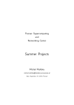
3.2 ‘Select A Flight’ Panel
This panel displays all of the active flights in the instance of FlightGear. You, the main
player, are listed as ‘Player’. Here you may select any flight in order to make it the currently
selected flight.
4
5
3.3 ‘Flight Info’ Panel
This panel displays all of the flight information from the currently selected flight including
flight speed, orientation, and position. The currently selected flight can be changed by selecting
a different flight from the ‘Select A Flight’ panel.
6
3.3 ‘Environment Info’ Panel
This panel displays weather information for the surrounding environment from your
flight’s perspective. This information will change based on the position of your flight. Information
that is displayed includes wind speed, temperature, and air pressure.
7
3.4 The Map Panel
This panel takes all of the flight information for all active flights in FlightGear, and uses
the information to display the flights on a map. This is a Google map and can be treated as
such. The capabilities of the map include the capabilities of any standard Google map. Flights
will be displayed as markers on the map and will change position and orientation as their flight
info is updated.
8
3.4.1 Center on selected
The map has an added button called ‘Center On Selected’ that centers the map on the
currently selected flight.
3.4.2 Toggle Flight Zone
The map also has a button that toggles a circle in which whose radius the FlightGear
server will send flight information for other flights. The radius of the flight zone is 100 nautical
miles. Any flight who enters the flight zone will be displayed and tracked by FlightTracker.
9
3.5 Logs
Any flight who has entered the flight zone mentioned earlier will be tracked by
FlightTracker regardless of whether or not that flight is still in the flight zone or not. All
multiplayer flight information is stored in logs that are kept by FlightTracker. These logs display
all of the selected flight’s past flights with starting and ending times as well as periodic time
stamps that also include flight position. The available logs can be found in the drop down log
menu option.
10
The logs that are displayed will look like this:
11
3.6 Connection Speed
The rate at which FlightGear sends messages to the ActiveMQ broker and subsequently
are received by FlightTracker can be modified. Using a menu option, a dialog window will be
displayed which allows you to enter any time interval at which you wish to receive messages
from FlightGear.
12
4. Admin Manual
This section of the administrator manual is designed to assist with implementing
ActiveMQ into a program and understanding the implementation of the components of
FlightTracker and CFD.
5. ActiveMQ
5.1 Broker
Programs using ActiveMQ require the broker to be running. The broker can be
downloaded off the ActiveMQ website. To change the port numbers that the broker uses,
navigate to the file at “../conf/activemq.xml”.
<transportConnectors>
<!-- DOS protection, limit concurrent connections to 1000 and frame size to 100MB -->
<transportConnector name="openwire"
uri="tcp://0.0.0.0:61616?maximumConnections=1000&wireFormat.maxFrameSize=104857600"/>
<transportConnector name="amqp"
uri="amqp://0.0.0.0:5672?maximumConnections=1000&wireFormat.maxFrameSize=104857600"/
>
<transportConnector name="stomp"
uri="stomp://0.0.0.0:61613?maximumConnections=1000&wireFormat.maxFrameSize=10485760
0"/>
<transportConnector name="mqtt"
uri="mqtt://0.0.0.0:1883?maximumConnections=1000&wireFormat.maxFrameSize=104857600"/>
<transportConnector name="ws"
uri="ws://0.0.0.0:61614?maximumConnections=1000&wireFormat.maxFrameSize=104857600"/>
</transportConnectors>
FlightGear in the Flight Simulator Suite uses the “openwire” transport connector
and the Flight Tracker GUI uses the “stomp” transport connector.
5.2 ActiveMQ Producer
Before starting either the ActiveMQ producer or consumer, the library must be
initialized. This is done (C++) by doing:
activemq::library::ActiveMQCPP::initializeLibrary();
and then the corresponding shutdown statement:
activemq::library::ActiveMQCPP::shutdownLibrary();
First a connection factory must be made. This is done with the statement:
auto_ptr<ActiveMQConnectionFactory> connectionFactory(
new ActiveMQConnectionFactory(brokerURI));
The “brokerURI” argument in this statement is the location of the broker. This
string would have the format “failover://(tcp://localhost:61616)”. After the connection
factory is made, a connection must be made.
13
m_connection = connectionFactory->createConnection();
m_connection->start();
The connection is then used to create a session.
session = connection->createSession(ACKNOWLEDGE_MODE);
Now, the destination object must be created. Either a topic or queue can be created.
destination = session->createTopic(destURI);
destination = session->createQueue(destURI);
A topic is used for the publish and subscribe method. This means that when a
producer pushes a message to a topic, all connected consumers will get a copy of the
message. A queue is used for the load balancer method. This means that when a
producer pushes a message to a queue, only one connected consumer will receive that
message. The “destURI” argument is the name of the topic or queue the producer is
pushing to.
Finally, the producer object can be created.
producer = session->createProducer(destination);
producer->setDeliveryMode(DeliveryMode::NON_PERSISTENT);
Sending a message is simply done by calling the send method on the producer object.
5.3 ActiveMQ Consumer
Creating an ActiveMQ consumer is done the same way as the producer. The
only difference is that a onMessage function is needed for when the consumer receives
a message.
consumer->setMessageListener(this);
This sets the current class as the message listener. Once the “onMessage”
function is overridden, the created function will then be called when the consumer
receives a message.
6. FlightTracker
It is possible to implement the different functionalities of FlightTracker using the
following guidelines.
6.1 Connection to ActiveMQ Broker
The FlightTracker program is connected to FlightGear through its use of
ActiveMQ’s broker. This connection allows the program to swap messages with
FlightGear in order to display the information and also to modify FlightGear. The
connection to the broker is made through the use of the library: Stompy. Within
FlightTracker’s Python source code lies some key implementations of this library.
conn2.set_listener('', MyListener(conn2,frame))
conn2.start()
conn2.connect(login=user,passcode=password)
14
conn2.subscribe(destination="TEST.FOO", id=1, ack='auto')
These lines of code allows the python program to start-up a connection to the broker and
also to subscribe to a certain queue on the broker where it will receive its messages
from.
A connection can also be made to send messages to the broker:
conn = stomp.Connection(host_and_ports = [(host, port)])
conn.start()
conn.connect(login=user,passcode=password)
conn.send(body = dlg.text.GetValue(),destination='MESSAGE_INTERVAL')
6.2 Utilization of Wx.Python
FlightTracker is made using WX.Python. Wx.Python is a Python extension for the
popular Wx.Widgets library written in C++.
Here is an example of Wx.Python being used to initialize the main frame for
FlightTracker:
super(FlightTracker, self).__init__(parent, size=(1024,700), style =
wx.DEFAULT_FRAME_STYLE)
self.currentDisplayFlight = "Player"
self.menubar = wx.MenuBar()
self.fileMenu = wx.Menu()
self.optionsMenu = wx.Menu()
self.connectionMenu = wx.Menu()
self.fileMenu.Append(EXIT, 'Exit', 'Exit')
self.connectionMenu.Append(CONNECTION,'Edit Connection','Edit
Connection')
self.menubar.Append(self.fileMenu,'File')
self.menubar.Append(self.optionsMenu,'Logs')
self.menubar.Append(self.connectionMenu,'Connection')
Wx.Python allows for very fast prototyping and functionality development and is easy to
learn and use making future development much simpler.
For further information, here is the website for Wx.Python: http://www.wxpython.org/.
And here is the helpful wiki for Wx.Python: http://wiki.wxpython.org/.
6.3 HTML and Javascript in Python
One key feature of FlightTracker is its ability to utilize Google Maps in python.
This feature is made possible by functionality provided by Wx.Python.
15
Here we can see an html page that is used to display the Google Map, being placed into
a sizer in the Map Panel of FlightTracker:
#set html page to be the one created from the javascript
self.parent.html_view = wx.html2.WebView.New(self)
dir_name = os.getcwd()+"/test.htm"
self.parent.html_view.LoadURL(dir_name)
GPSSizer.Add(self.parent.html_view,1,wx.EXPAND)
self.SetSizer(GPSSizer)
This HTML page is updated periodically in FlightTracker and is displayed in the Map
panel. Within the HTML code, JavaScript is also embedded. The JavaScript is used to
implement the Google Maps JavaScript API. The HTML and Javascript are both
managed through the class ‘PyMap.py’ which contains all of the code encapsulated
within a string. Here is an example:
self.html = """
<!DOCTYPE html>
<html>
<head>
<title>Accessing arguments in UI events</title>
<meta name="viewport" content="initial-scale=1.0, user-scalable=no">
<meta charset="utf-8">
<style>
html, body, #map-canvas {
height: 100%%;
margin: 0px;
padding: 0px
}
</style>
%s
</head>
<body>
<div id="map-canvas"></div>
</body>
</html>
""" % self.GoogleMapPy()
The method GoogleMapPy() referenced above contains all of the JavaScript used to
implement the Google Maps API. Here is some example JavaScript code where a new
marker is added to the map:
//add flight marker
function addMarker(lat, lon,name) {
var location = new google.maps.LatLng(lat,lon);
symbol = {
path:
google.maps.SymbolPath.FORWARD_CLOSED_ARROW,
scale: 4,
strokeWeight: 3,
16
strokeColor: 'red',
rotation: 0
};
var marker = new google.maps.Marker({
position: location,
map: map,
icon: symbol,
title: name,
optimized: false,
pastLat: lat,
pastLon: lon,
animation: google.maps.Animation.DROP,
selected: false
});
markers.push(marker);
}
The JavaScript methods that control the map can be called from the Python code. Here
is an example where a marker on the map is updated:
#update the GPS map
scriptString = """updateMarker(%s,%s,"%s",%s,"%s")""" %
(str(lat),str(lon),str(name),str(heading),selected)
self.MainPanel.html_view.RunScript(scriptString)
The JavaScript method call is placed into a string and sent to a Python function which
sends the command to the map.
7. Computational Fluid Dynamics
We have attempted to build a program that models the motion of the air. The
program design is composed of two subprograms tasked with the responsibilities of
computing the flow-field variables and displaying a graphical representation of the
simulation. The Solver subprogram is the computational engine; the Visualizer
subprogram maintains a scene graph and uses the results of the Solver to define the
vertex shaders and primitive types. This document is concerned with the Solver
program. We will begin with an overview of the process, followed by a brief analysis and
derivation of the equations. Finally we will document the organization of the code.
7.1 Overview
There are two primary steps of the Solver process:
1.
Discretization of the partial differential equations and auxiliary equations (i.e. the
initial conditions and boundary conditions) into a system of algebraic equations
2.
Implementation of numerical solvers to compute the solution of the system of
algebraic equations.
Before converting the partial differential equations into an algebraic form in the
discretization step, we must first decide on a discretization method. There are a variety
of methods we may use to accomplish this task; in this work we focus on the finite
17
volume method. The finite volume method is a discretization of the integral form of the
conservative equation. The computational domain is subdivided into a number of control
volumes. The governing equation is then discretized into an algebraic expression
representative of the conservation of the flow field variables for each control volume.
Polynomial interpolation and numerical integration are used to obtain an algebraic
expression for the quantities that express spatial change. In order to ensure that the
flow-field variables are conserved, we average the flux calculations of neighboring
volumes to obtain the flux across any face bounding two control volumes. Discretization
in time is achieved via an implicit finite difference method.
The Solver program was organized in such a way to maximize flexibility. Any task that
can be implemented with a variety of different strategies is exported to a class.
Eventually, the goal is to create a fully templated program, where the management
classes are templates with method or model parameters. Currently the program
leverages inheritance to accomplish the use of different methods. Incorporating
templates into the design will allow us to use different objects to accomplish the same
task. Inheritance should be used only for objects of the same type with additional or
specialized functionality. For example, we mentioned that the discretization step can be
accomplished by a variety of methods. Currently, the program is arranged such that a
discretization method is a derived class of an abstract class called ‘SpatialSolver’.
(Admittedly, that title is not entirely accurate and should be changed to a more
appropriate descriptive title such as ‘DiscretizationMethod’.) A portion of the program is
illustrated below in the form of a class diagram. A more detailed diagram is included at
the end of the document.
18
7.2 Analysis and Derivation of Governing Equations
In this section we analyze the equations that model the motion of the air. We
begin the analysis with the Reynolds Averaged Navier Stokes (RANS) equation, which is
a variation of the Navier Stokes equation obtained by replacing the velocity with an
averaged velocity plus instantaneous velocity component. The RANS equations can be
expressed as the following equation
[1]
where FI and FV are the inviscous and viscous flux matrices, respectively. They are
defined
[
]
[
]
19
̅
̅
̅
̅
,
,
̅
̅
(
))
̅)
( ( ̅̃
)
(
where
is the Kronecker delta function, and wi is the velocity component of the ith
dimension, where i = 1 indicates the x-axis, i =2 indicates the y-axis, and i = 3 indicates
the z-axis.
denotes a viscous stress in the j direction exerted on a plane
perpendicular to the i-axis. An illustration of the physical meaning of these variables is
depicted in the figure below.
U is the solution vector of conservative variables, defined
̅
̅
̅
̅
( ̅̃ )
A bar over the variable is used to indicate that the time average. The time average of a
function is defined
̅
∫
First we integrate [1] over the volume of the fluid container, the domain of the problem,
to obtain an equation in integral form.
20
∰
∰
∰
∰
[2]
Now we use the divergence theorem, which states
∰
∯
∯
∯
To rewrite [2]
∰
∰
[3]
The average of a function is
̅
∰
We further simplify [3] by replacing the volume integrals with the average to obtain
̅
̅
∯
∯
7.3 Class List
Problem
The problem class is the highest level management class of the Solver program that
provides the environment for the computation process. Upon completion, the interface
between the user and the program will communicate with Solver by setting the methods
and parameters of the Problem. The Problem class is responsible for integrating the time
stepping with the spatial discretization. It is also responsible for loading initial conditions
and boundary conditions that define a simulation instance. The mesh generation type
and duration of the simulation is also defined in this class.
ODESolver
The ODESolver is the abstract class of which all numerical methods that solve systems
of ODEs are derived from. Currently the classic fourth order Runge Kutta is
implemented. However, since fourth order accuracy is too computationally expensive in
a three dimensional implementation of the finite volume method, a second order method
must be implemented. Currently Lax-Wendroff is also derived from ODESolver, but this
is an error. The Lax-Wendroff method is a numerical method used for the discretization
of hyperbolic partial differential equations. It is not a method used for solving ordinary
differential equations.
FiniteVolumeMethod
The FiniteVolumeMethod (FVM) class is responsible for managing all system calls
related to the spatial discretization. It does not perform any of the actual processing.
Instead, it manages the objects responsible for performing each step of process. There
are three objects that the FVM class manages: Mesh, Face, and Volume. It calls on
these classes to generate the grid, construct the volumes, and compute the fluxes. For
each step in time, the FVM method computes the flux matrices for each volume cell by
iterating through the list of Volume references and updating them.
Mesh
21
The Mesh class generates the grid that covers the domain of the problem. It defines the
faces in terms of these grid points and volume cells, or 'control volumes' in terms of
enclosing faces. The purpose of maintaining a separate object for the completion of this
task is to allow for the use of different meshing algorithms.
Face
A Face object manages the computations that correspond to the passage of fluid across
a face in the mesh. In this context, the computations are calls to the flux function. Flux is
a function of the conservative variable solution vector.
Volume
The Volume object manages the calls required to solve the governing equations for a
single control volume. The functions of this class handle the computations of polynomial
interpolation and numerical integration that are signature steps of the finite volume
method. Since we are solving for a multidimensional quantity of multivariate functions,
polynomial interpolation is too expensive. Instead we use a single data point, the value
at the centroid of the volume, to approximate the integral using the midpoint rule.
Currently, we confine ourselves to cube shaped volumes; we will always have six square
faces bounding a volume.
∯
∑
∫
∫
∑
BACK MATTER
Vocabulary
Cell. A cell is a subset of the grid points of a mesh. The intersection of all cells is empty,
and the union of all cells covers the entire domain.
Face. A face is a two dimensional bounding surface of a volume.
Mesh. A mesh is a set of vertices, edges, and faces.
Volume. A volume is polyhedral contained within the domain of the problem. Volumes of
a domain may overlap. The defining characteristic of a volume is that it is the space for
which the solution vector of conservative variables is solved.
Class Diagram: Solver
22
Class Diagram: Visualizer
Cells – The cells class creates a mesh Geode. A Geode in Open Scene Graph is the
(leaf) node of a scene graph that contains the geometrical data.
Face – The struct that holds vertex information of one face of a mesh polyhedra
GraphicsWindow – This class is an osgViewer that is embedded in a wxWidgets. It is
responsible for handling the graphics context (i.e. where to draw) of the scene graph.
MainFrame - The frame classes contain views and the widgets the user interacts with to
communicate with the application. Currently this is only relevant to menus in the toolbar,
23
as the event handlers for the user interaction with the osg models are defined in
OsgCanvas
OsgApp – This is the main enry point of the application from which the main frame is
launched.
OsgCanvas – This class defines all event handlers used to interact with the model
objects in the main view.
ViewMesh - The View classes contain the interface definitions to different child windows
and dialog boxes. View classes are associated with a frame class. ViewMesh in
particular hosts the osgViewer. It is responsible for setting the scene data.
A sample screenshot:
24
25