Download VRSimVer2.0 User Manual

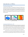
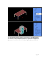
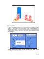
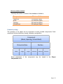
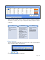
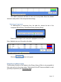
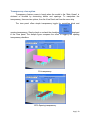
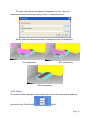
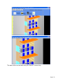
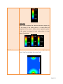
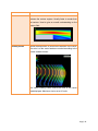
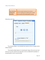
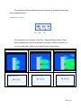
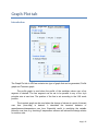
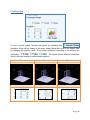
VRSimVer2.0 User Manual
INTRODUCTION TO VRSIM .................................................................................................................5
VIRTUAL ROOM SIMULATOR-VRSIM................................................................................................................. 5
COMPUTATIONAL FLUID DYNAMICS – CFD ........................................................................................................ 5
ROLE OF VRSIM SOFTWARE............................................................................................................................. 6
WHO SHOULD USE THE SOFTWARE? ................................................................................................................. 6
WHERE VRSIM APPLIES .................................................................................................................................. 6
HOW TO USE THE SOFTWARE? ......................................................................................................................... 7
GEOMETRY SETUP..............................................................................................................................8
INTRODUCTION ............................................................................................................................................. 8
DOMAIN GEOMETRY SETUP ............................................................................................................................ 8
SETTING THE DOMAIN GEOMETRY.................................................................................................................... 8
OBJECT GEOMETRY SETUP .............................................................................................................................. 9
SETTING OBJECT GEOMETRY ......................................................................................................................... 10
MESH .............................................................................................................................................. 16
INTRODUCTION ........................................................................................................................................... 16
NUMBER OF CELL ........................................................................................................................................ 16
BIAS FACTOR .............................................................................................................................................. 17
MINIMUM GAP SPACING ............................................................................................................................... 17
GENERATING MESH ...................................................................................................................................... 17
WARNING DISPLAY....................................................................................................................................... 18
BOUNDARY CONDITIONS SETUP ....................................................................................................... 19
INTRODUCTION ........................................................................................................................................... 19
THERMAL SETUP.......................................................................................................................................... 20
OPENING TYPES .......................................................................................................................................... 21
VELOCITY SETUP .......................................................................................................................................... 21
DIFFUSER MODE .......................................................................................................................................... 22
SPECIFIED FLOW RATE................................................................................................................................... 22
SPECIFIED PRESSURE..................................................................................................................................... 22
SOLVER CONTROLS .......................................................................................................................... 23
INTRODUCTION ........................................................................................................................................... 23
SIMULATION MODE ..................................................................................................................................... 23
HEAT TRANSFER MODEL ............................................................................................................................... 24
BUOYANCY MODEL ...................................................................................................................................... 24
IAQ MODEL ............................................................................................................................................... 24
ITERATION SETUP ......................................................................................................................................... 24
Page | 1
TRANSIENT PARAMETERS .............................................................................................................................. 26
RUNNING THE SIMULATION ............................................................................................................. 27
SIMULATION START\END .............................................................................................................................. 27
TERMINATING SIMULATION ........................................................................................................................... 28
SHAPE LIBRARY EDITOR.................................................................................................................... 29
INTRODUCTION ........................................................................................................................................... 29
GROUP AND OBJECT TREE STRUCTURE AND OPERATIONS .................................................................................... 29
Adding new group\object ................................................................................................................... 30
Deleting group\object ......................................................................................................................... 31
Copy and paste object ......................................................................................................................... 31
Duplicating group................................................................................................................................ 34
GEOMETRY SETUP........................................................................................................................................ 35
Adding a Component .......................................................................................................................... 36
Deleting a Component ........................................................................................................................ 37
BOUNDARY CONDITION SETUP ....................................................................................................................... 37
IMPORT & EXPORT DATABASE FILE ................................................................................................................. 39
Export\Create update file.................................................................................................................... 39
Import\Update database from file...................................................................................................... 42
PERSISTENT MODE ...................................................................................................................................... 43
ENVIRONMENT ................................................................................................................................ 44
INTRODUCTION ........................................................................................................................................... 44
MAIN VIEW MOUSE\KEYBOARD CONTROL ....................................................................................................... 45
BACKGROUND\ATMOSPHERE COLOR .............................................................................................................. 46
WALL COLOR .............................................................................................................................................. 47
FLOOR COLOR ............................................................................................................................................. 48
TRANSPARENCY VIEW OPTION ........................................................................................................................ 50
SCALE DISPLAY ............................................................................................................................................ 51
VIEW PANE MODE ....................................................................................................................................... 52
ADVANCED TOOLS ........................................................................................................................... 54
REPORTING SIMULATION SETUP ..................................................................................................................... 54
ADVANCED SOLVER SETUP ............................................................................................................................. 55
General tab ......................................................................................................................................... 57
Fluid Property ...................................................................................................................................... 58
IAQ Input Parameters ......................................................................................................................... 58
Indoor Air Quality (IAQ)....................................................................................................................... 58
Flow Model tab ................................................................................................................................... 60
Transient setup ............................................................................................................................... 60
Flow model...................................................................................................................................... 60
Page | 2
Linearization model ........................................................................................................................ 63
Buoyancy model.............................................................................................................................. 63
Initial Condition tab............................................................................................................................. 64
Matrix Solver tab................................................................................................................................. 64
Relaxation tab ..................................................................................................................................... 65
Limits tab............................................................................................................................................. 66
INTRODUCTION TO VRVIEW ............................................................................................................. 67
VIRTUAL ROOM VIEWER-VRVIEW .................................................................................................................. 67
VRVIEW AS A POST-PROCESSOR ..................................................................................................................... 68
A TASK SPECIFIC SOFTWARE ........................................................................................................................... 69
HOW TO USE THE SOFTWARE? ....................................................................................................................... 70
FILE LOADING .................................................................................................................................. 71
COMPONENTS OF SOLUTION FILES .................................................................................................................. 71
LOADING FILE USING “AUTOLOADER” FEATURE ................................................................................................ 72
LOADING FILE USING “LOAD FILES” FEATURE .................................................................................................... 73
DISPLAY TAB .................................................................................................................................... 75
INTRODUCTION ........................................................................................................................................... 75
VARIABLES TAB............................................................................................................................................ 76
VIEW MINI TAB............................................................................................................................................ 78
OPTION MINI TAB ........................................................................................................................................ 83
Room View features ............................................................................................................................ 83
Object View features ........................................................................................................................... 84
ANIMATION MINI TAB................................................................................................................................... 84
Animation control ............................................................................................................................... 85
Video streaming control ...................................................................................................................... 86
GRAPH PLOT TAB ............................................................................................................................. 87
INTRODUCTION ........................................................................................................................................... 87
PROFILE GRAPH ........................................................................................................................................... 88
TRANSIENT GRAPH ....................................................................................................................................... 89
SAVING PLOTTED GRAPH ............................................................................................................................... 91
Save As Image ..................................................................................................................................... 91
Save As File .......................................................................................................................................... 91
REPORT TAB .................................................................................................................................... 93
INTRODUCTION ........................................................................................................................................... 93
IMAGE PANE ............................................................................................................................................... 94
Adding image ...................................................................................................................................... 94
Page | 3
Browsing image................................................................................................................................... 95
Deleting image .................................................................................................................................... 96
Save image to folder ........................................................................................................................... 97
REPORT DETAILS .......................................................................................................................................... 98
Create a report file .............................................................................................................................. 99
STREAMLINES ................................................................................................................................ 101
INTRODUCTION ......................................................................................................................................... 101
STREAMLINE OPERATIONS ........................................................................................................................... 102
Show\Hide streamline ....................................................................................................................... 102
Position\Coordinate of streamline .................................................................................................... 102
Adding streamline ............................................................................................................................. 102
Remove streamline ........................................................................................................................... 104
Clear all streamline ........................................................................................................................... 104
STREAMLINE ANIMATION ............................................................................................................................ 105
STREAMLINE DENSITY ................................................................................................................................. 105
ADDITIONAL TOOLS ....................................................................................................................... 107
MAIN VIEW CONTROLS ............................................................................................................................... 107
PREDEFINED VIEW CONTROL ........................................................................................................................ 108
CUTTING PLANE CONTROL ........................................................................................................................... 108
Show\hide the cutting plane ............................................................................................................. 108
Moving the cutting plane .................................................................................................................. 108
SHOW\HIDE PANE VIEW ............................................................................................................................. 109
Page | 4
Introduction to VRSim
Virtual Room Simulator-VRSim
Virtual Room Simulator (VRSim) is a Computational Fluid Dynamics (CFD) software used to
predict air flow movement and heat transfer occurring from air-conditioning units within a space.
The software will solve the fluid and heat transfer numerically and predicts the solution from a
given model. This VRSim code was initiated from a joint collaboration project between OYL
Research & Development Center Sdn Bhd with the CFD team from Universiti Tenaga Nasional,
Malaysia. The concepts originated from the project were then extended to the current version of
this VRSim software.
Example contours of air flow
Computational Fluid Dynamics – CFD
The two traditional approaches to engineering are the analytical approach and experimental
approach. Computational Fluid Dynamics (CFD) added another dimension to engineering study
by using computer and numerical method to solve engineering problems. CFD also plays the
role as a complementary approach to both analytical solution and experimental results. While it
is true that CFD can never be viewed as a total substitute for experimental result or analytical
study; if it is used correctly, it is on par with the trustworthiness of the other two approaches.
CFD originated from the aeronautical and aerospace industry and it has spilled into other
critical applications such as automobile, turbo-machinery, bioengineering, and electronic cooling
system, and the list keeps expanding rapidly. Nowadays, CFD is commonly found in automobile
Page | 5
companies such as Proton, Toyota and others. This is due to its role in reducing cost and
speeding up the design to production time cycle.
Role of VRSim software
VRSim is useful when the air flow pattern and the heat transfer of the indoor condition or
outdoor conditions need to be studied. The prediction can be used to optimize design or to
simply detect potential trouble areas and troubleshoot existing configuration.
For example, to install outdoor units with irregular configuration in a hot and humid
tropical country such as Malaysia or Singapore, there is a risk that the units may get
overheated. Where analytical and experimental solution is time consuming and costly, VRSim
can be used to predict the flow pattern and heat transfer behavior of the air as the unit is
running in extreme conditions. With VRSim, the analysis can be done with virtually no additional
cost and using less time. In short, VRSim project emulates the concept of CFD in reducing cost
and shortening analysis time for design applications.
Who should use the software?
HVAC engineers! VRSim is in fact customized CFD software. VRSim is made specifically for
applied HVAC engineers in minds. While the learning curve of the software is simple enough so
that it can be understood and operated by any layman, it still needs actual design engineers to
analyze the software simulation results. This differentiates the VRSim as a product which is
made for engineers to a software product made for the ordinary layman.
Where VRSim applies
There are three common situations where you might need to use VRSim:
i)
New design validation.
This is when the results are used to support project proposals to the
customer or if uncertain how the design will affect the air flow and heat
transfer phenomena.
ii)
Troubleshooting old design.
Page | 6
This is when there are problems with the previous design and it is desired
to understand why the failure of the design occurs.
iii)
For gaining customer trust.
Using scientific approach benefits in gaining customer trust on user
professionalism and work quality.
Geometry setup
How to use the software?
A tutorial has been provided with the software to initially introduce the basic interface in VRSim.
Then, a series of step-by-step tutorials on how to setup the simulation and analyze the result is
presented based on the user level.
This user manual adds further explanation on the mechanics of the VRSim software to
complement the tutorial guide.
Page | 7
Geometry Setup
Introduction
The geometry setup is divided into two main parts. Domain Geometry setup and Object
Geometry setup.
Domain Geometry Setup
The Domain geometry refers to the overall domain that defines the limits of the
computational boundary of the solver. For example, if you are simulating a flow in a
rectangular closed room, the domain is the walls of the room. For cases of domain with
irregular shape, such as an “L” shaped domain, it can be build by first defining a
rectangular domain and later rectangular objects (blockades) can be inserted to form
the desired domain.
“L” shaped domain.
Setting the Domain Geometry
To set the size of the domain geometry, click the
Domain Settings window will appear.
access button and the Flow
Page | 8
The dimension of the domain then can be set according to width (along the X-axis),
length (along the Y-axis), and height (along the Z-axis) dimension.
Object Geometry Setup
The object geometry refers to the blockade and opening components that can be set
inside the domain. It represents real life object such as chairs, sofa, bed, table, human
body, etc..., in the geometry model. The object geometry is divided into two types, which
are the Custom type and the ShapeLib type.
The custom type is further broken into either block or opening. It is useful to
represent geometries which are specific to a particular case such as atmospheric
openings on the domain wall or pillars to a specific size in a hotel lobby.
The ShapeLib type is a unique geometry type where an object is represented by
a collection\combination of block, opening and virtual block\opening. It shows geometry
that are already built in the Shape Library Editor and shown as a single entity in the
ObjectBrowser window. Its usage is for common shapes which will be used repeatedly
in other cases. Examples of ShapeLib object include Wall Mount unit model, SL outdoor
unit model and a standing human model.
Page | 9
Blocks
Custom
Openings
Blocks
Object
+
Openings
ShapeLib
+
Virtual Block\Opening
Setting Object Geometry
To set the object geometry, click the
window will appear.
access button and the ObjectBrowser
Page | 10
Adding objects
Custom type
In the ObjectBrowser window, go to the Custom Object tab.
Set the dimension of the block or opening (where one of the size
field will hold the zero value). Click the
button and
a block\opening can be seen in the model viewer and object list.
ShapeLib type
In the ObjectBrowser window, go to the Library Object tab.
Page | 11
Choose the Object Group
from the
dropdown list. Example, Furniture group. Choose an Object
Name
available in this group, e.g.
Cabinet. Click the
button in the tab and a cabinet
object will be added to the model viewer and the list.
Deleting
Choose one of the objects desired to be deleted from the object list in
objects
the ObjectBrowser.
Click the
button. The object is deleted from the list and the
model viewer.
Page | 12
Editing Objects
Position
Set the position coordinate following the Xpos, Ypos, Zpos fields in
the object list. Click the
button to update the change.
Dimension
Choose one of the objects desired to be edited from the object list in
the ObjectBrowser.
Go to the Custom Object tab and change the dimension field values.
Page | 13
Click the
button to update the change.
NOTE: Dimension edit and color edit is only applicable for Custom
type object.
Color
Choose one of the objects desired to be edited from the object list in
the ObjectBrowser.
Page | 14
Go to the Custom Object tab and click the
button.
Change the color to the desired color in the color dialog.
NOTE: Dimension edit and color edit is only applicable for Custom
type object.
Page | 15
Mesh
Introduction
Loosely, mesh is referring to the result of the process of breaking up a physical domain
into smaller sub-domains. This process is also termed as meshing process,
discretization (from the word discrete), and grid generation. The code which generates
the mesh computationally is called grid generator or mesher.
VRSim is using a fully-automated mesh generator with user defined input. The
type of mesh in used is a axis aligned Cartesian mesh type. This type of mesh has the
advantage of fast generation, robust and orthogonal cell faces. It also contributes to
high accuracy result.
The user inputs for the mesher are the minimum number of cells, bias factor, and
minimum gap spacing.
Number of Cell
The number of cells refers to the number of cells in each axis direction (X/Y/Z).
However, the mesher just uses the number as a guideline. The final number of cells
generated may differ from what is inputted by the user. This is indicated on the top of
the window as shown.
Page | 16
Bias Factor
The bias factor controls how the nodes of the cells are to be clustered. Bias factor of
1.00 indicates an evenly spaced cell size. Values other than 1.00 will stretch the
distribution of the nodes along the X/Y/Z axis.
Minimum gap spacing
When a small gap is detected in the geometry, this option sets the minimum number of
nodes to be inserted in such gap.
Generating mesh
To set the mesh properties, click the
window will appear.
access button and the Mesher
Set the mesh property accordingly and click the Apply button. The Mesher window
mode changes to the display mode with the result mesh shown in the model viewer.
Page | 17
Moving the Mesh Plane slider control will accordingly move the mesh plane in the model
viewer.
Warning display
The mesher will occasionally display warning messages to indicate low quality mesh
generated in the model. While is not necessary to have zero warning error message in a
particular mesh result, too many warning indicates severe geometry misplacement.
Page | 18
Boundary Conditions Setup
Introduction
The boundary condition can be viewed by clicking the
BCs window will appear.
access button. The
There are three BCs tab components that can be set by user. They are the
Obstacle BC (for custom Block BC), Opening BC (for custom Opening BC) and
Enclosure BC (for wall\enclosure of domain BC).
Page | 19
For all of the components the thermal setup can be set by user. However, the
openings have extra parameters that will be enabled according to the opening type
being set by user.
Summary on the structure of BC setup is shown here.
Blockade BC
Thermal
Setup
Enclosure BC
Thermal
Setup
Opening
Type
BCs
Components
Thermal
Setup
Opening BC
Velocity
setup
Diffuser
Mode
Spec.
Flowrate
Spec.
Pressure
Thermal Setup
Thermal setup sets the thermal condition of the blocks, opening, or enclosure\wall of
domain.
Specified Heat Load
The default setting of “Specified Heat Load” condition with zero value sets the
blocks as pure blockade with no heat source and opening as pure opening with
no cooling or heating effect through it. If the heat load applied across the
opening, block or enclosure\wall surface is constant (known), set the thermal
setup to this option. Specify the value in the field provided.
Page | 20
Specified Temperature
If the temperature applied across the opening, block or enclosure\wall surface is
constant (known), set the thermal setup to this option. Specify the value in the
field provided.
Opening Types
Inlet
Choose this type of opening if the opening is acting as an inlet. Only the thermal
setup, flow setup (velocity, diffuser mode) and suctionID feature is enabled for
this option.
Outlet[Pressure]
Choose this type of opening if the opening is acting as an outlet with known
(fixed) pressure. Only the pressure field is enabled for this option.
Thin Solid
Choose this type of opening if the opening is modeling objects such as glass
pane, closed window. Only the thermal setup is enabled for this type of opening.
Atmospheric Boundary
Choose this type of opening to represent atmospheric boundary where the
direction of the flow is principally unknown or not constant.
Outlet[Mass flow]
Choose this type of opening to represent outlet with constant mass flowrate. Only
the mass flow rate field is enabled in this option.
Velocity setup
Flow rate
The flow rate of the openings in CFM (Cubic Feet per Minute) can be set to
represent the velocity of the fluid.
Specifying Angle
Page | 21
The velocity vector angle is specified based on the reference to the principal axis
(X/Y/Z-axis). This is illustrated in the figure below.
Only two angle needs to be supplied by the user. For example, if the opening is
lying on the XY-plane, the angle of the vector to the principal z-axis is blanked and
resolved by VRSim. The proper direction will be set by VRSim based on the type of the
opening. This is to reduce ambiguity and input error by user.
Diffuser mode
Enable the diffuser checkbox to specify inlet openings which have a diffusing flow
pattern. The diffusing pattern is specified in central radial fashion with a specified
diffusing angle. The specified diffusing angle is measured as shown in the figure below.
Inlet opening
Diffusing angle
Specified flow rate
Specify the fixed flow rate value in this field. Applicable only to Outlet[Mass flow]
opening type.
Specified pressure
Specify the fixed pressure value in this field. This is applicable only to Outlet [Pressure]
and Atmospheric Boundary opening type.
Page | 22
Solver Controls
Introduction
Solver refers to the code which runs to solve the fluid flow problem submitted to it. It can
be said to be the “brain” part of VRSim software. The input of the solver is the geometry
definition and boundary condition of the said geometry.
The solver control window acts as a command center which decides how the
“brain”\”engine” is to be controlled. To view the solver control window, click the
access button. A basic solver control window will appear.
Simulation Mode
The simulation mode offers two options. “New Simulation” option offers fresh simulation
iteration. This option is the choice when a simulation is to be done for the first time or
when a new simulation iteration starting from zero is to be overwritten over an old
simulation run.
Page | 23
The “Continue…” option is used when the simulation is to be continued from a
last simulation. For example, a simulation has been run from 1 to 100 iterations. To
produce a simulation running from 1 to 300 iterations, simply change the mode to
“Continue…” and just add another 200 iteration to the existing one. Thus, there is no
need to repeat the first initial 1 to 100 iterations to obtain a continual of the simulation.
Heat transfer Model
Turn on this option if the heat transfer (temperature distribution) of the fluid is to be
simulated together with the fluid flow.
Buoyancy Model
Turn on the option if the buoyancy behavior (hotter fluid rise, colder fluid sinks,
phenomena) is to be simulated together with the fluid flow. The reference temperature
in this section refers to the set ambient temperature. (Example: 35 degree Celcius
ambient air temperature, during noon time in Malaysia).
IAQ Model
Turn on this option if the Indoor Air Quality (IAQ) parameters are to be calculated. The
result will be displayed in terms of distribution of scalar parameters such as Draught
Risk (in percentage), Draft Temperature, Predicted Percentage Dissatisfied (PPD), and
Predicted Mean Vote (PMV).
Iteration setup
The iteration setup has two main parameters\criteria. They are the “number of
iteration” and the “convergence criteria” parameters.
The “number of iteration” is termed differently in steady and unsteady mode. In
transient state simulation, it is termed as “Maximum Iteration per time step” which
represents the maximum iteration that can be reached for each time-step. Optimal value
is around 100 iterations.
Page | 24
In a steady-state simulation it is termed as “Maximum iteration”, as there is only
one single time-step in a steady-state simulation. Optimal value is around 300 to about
1000 iterations depending on the complexity of the model. For further example on
steady-state and transient simulation, see Advanced Solver Setup section.
The “convergence criterion” is the largest error level that needs to be achieved
for the solution to be considered as “converged”.
For each time step, if one of the two criteria is already met, the simulation will
stop and jump to the next time –step.
Page | 25
Transient parameters
The transient parameters control the time step sequence for the transient simulation.
“Time step size”
Definition:
It is the time step difference for each time step.
Example:
“Time step size” with a value of 0.1 will produce time sequence
0s, 0.1s, 0.2s, 0.3s….
“Number of time step”
Definition:
Contributes to the total number of time step applied for the solver. In a
relationship this gives:Total_time = (Number_of_time_step) x (Time_step_size).
For example, given a simulation with “Number of time step” of value 100;
Total_time = 100 x 0.1 =10s.
The time step sequence becomes,
0s, 0.1s, 0.2s, 0.3s…..9.9s ,10s.
“Save result at every”
Definition:
The parameter is a control for the solver to save the simulation result file at every
specified time-step level.
For example, using the default value of 5 for the parameter will give a sequence of:
Time step (s):
0.1s, 0.2s, 0.3s, 0.4s, 0.5s
…..9.9s ,10s
Time step Number
1,
2, 3,
4, 5(saved) ,…..99, 100(saved).
Thus, the final animated result sequence seen in the post-processor (VRView) is,
Time step (s):
0.5s, 1.0s, 1.5s, 2.0s …..9.5s, 10.0s.
Page | 26
Running the Simulation
Simulation Start\End
To start the simulation, click the
access button in the simulation panel.
Specify the folder where the result is to be saved.
The solver engine will start and shows the convergence plot simulation messages.
Page | 27
At the end of the simulation a pop-up window will appear.
A pop-up window will appear after the simulation has been completed. Click “Yes” to exit the
solver mode. If you clicked “No”, simply close the window of the solver mode to obtain your
result files.
Terminating simulation
To terminate the solver calculation, click the
access button.
Wait for the simulation to finish its last time-step iterations. This may take a few minutes.
If the simulation is to be terminated without the saving the last time step result, simply
close the solver window that contains the simulation residual plot etc...
Page | 28
Shape Library Editor
Introduction
To access the Shape_Library_Editor mode, go to “Shape Library” tab and click the
access button. The main view will change to the Shape_Library_Editor
mode.
The local principle (X/Y/Z) axis is displayed as a reference (shown in blue, red
and green). The reference coordinate for rotation and translation is always fixed to be at
the origin (coordinate; <0, 0, 0>) of the displayed axis.
Group and Object tree structure and operations
The display shows the database tree on the right side panel of the interface. The
database tree is a tree which represents the list of Group and its child objects. The
objects consist of three components which are the blocks, virtual block, and openings.
Each of these components has geometry parameters of size; width, length, height, and
Page | 29
position; (x,y,z) coordinate. At the same time, the components also have its
corresponding Boundary Condition parameters (except Virtual Block). A sample on the
tree structure is as shown in figure.
Database Tree
Indoor unit type A
Indoor Unit type B
Project: Sunrise Building
WM009966
CE3003
Case 1
Component
CE3004
Case 2
Geometry
Boundary
Condition
Adding new group\object
To add a new group to the tree list, click on any of the existing group and click
the Add button.
To add a new object to the tree list, click on any of the existing on object in the
desired group and click the Add button.
Page | 30
Deleting group\object
To delete\remove a desired object from the tree list, simply highlight the object
(by clicking on it) and click the Remove button. A pop-up window prompting the
action will appear. Click “Yes” to continue.
Warning: There is no “Undo” feature in the software. Ensure that the object
to be removed is the correct object.
Copy and paste object
i)
To a group list: To copy an object from a group A to another group B,
highlight and right click the mouse on the object to be copied. Click the
“Copy Object” option from the pop-up menu that appears.
Highlight and right click the target Group B where the object is to be copied to.
From the pop-up menu that appears, click the “Paste Object” option.
Page | 31
The object is then copied from Group A to the target Group B.
This is beneficial when a similar objects but with different group is to be
constructed. The copied object then can be easily edited accordingly.
ii)
Into an existing object: To copy an object A to another object B, highlight
and right click the mouse on the object to be copied. Click the “Copy
Object” option from the pop-up menu that appears.
Highlight and right click the target Object B where the object A is to be copied to.
From the pop-up menu that appears, click the “Paste Object” option.
Page | 32
The object A is then copied to object B (original name of object B is retained).
This operation is useful for duplicating objects into a single object, for example an
object where a few outdoor units are to be placed together (see sample figure).
Page | 33
Duplicating group
In cases where a whole group is to be edited and modified while the original
group is to be retained, a Group duplication feature is also available. For
example, a similar group of furniture for Europe market is to be redimensioned to
fit into a furniture group for Asia market. Start off by highlighting and right click
the original group.
From the appeared pop-up menu, click the “Duplicate Group” option. A new
duplicate group will then be created.
Page | 34
Limit on number of entries
Currently the number of entries of the database is limited to;
Component
Group list
Object list
Block
Opening
Virtual Block
Maximum limit
75 units
50 units per Group
100 units per Object
100 units per Object
100 units per Object
.
Geometry setup
The geometry of an object can be composed of three possible components. Each
component has two attributes, namely, dimension and position.
Component
(Block, Opening, Virtual Block)
Dimension\Size
Width
Height
Length
Position
XPosition
YPosition
ZPosition
These parameters of the components may be viewed in the Object
Components table.
Page | 35
Directly edit the parameter values to change or set any component’s dimension
and position. A summary on the type of components and its properties is shown
in the table.
Block
•Represent real physical
block
•Dimension field must not
be zero.
Virtual Block
•Represent virtual block or
opening in simulation.
•No real physical effect to
simulation.
•Usually used for realism
effect such as
representing"Grill", "Chair
Legs" etc...
•Good for showing objects
that has little to no
significance effect on the
flow in simulation.
Opening
•Represent real physical
opening
•Dimension need to be
represented correctly
(one of the dimension
field need to be zero)
Adding a Component
To add a component to the table list, choose the tab of the component (Block
Setup, Virtual Block Setup, Opening Setup).
Click the
button in the panel.
Page | 36
The added component will have a new row of entry fields. Enter the desired
dimension and position of the component accordingly.
Deleting a Component
To delete\remove a component from the table list, choose the tab of the
component (Block Setup, Virtual Block Setup, Opening Setup).
Ensure that the object to be removed is highlighted in the table.
Note: Highlight just one of the cells in the table.
Click the
button in the panel.
Boundary Condition setup
The Boundary Condition of the objects in the Shape_Library_Editor is only accessible in
this mode and not in the main viewer. Table below list the BC feature available for each
geometry components (see; Geometry setup).
Page | 37
Block
• Thermal BC
Virtual Block
• No BC setup
available
Opening
• Opening Type
• Thermal BC
• Velocity BC
• Diffuser Mode
• Specified Mass
Flowrate
• Specified
Pressure
To open the window for setting the Boundary Condition, click the “Boundary
Conditions-> Show Panel” option in the menu strip.
The Boundary Condition window will appear.
Page | 38
For further explanation on the Boundary Condition setup, see section: Boundary
Conditions.
Import & Export Database file
Export\Create update file
To view the Export_Shape_Library_Editor window, go to the Shape_Library
tab\panel and click the
button.
The Export_Shape_Library_Editor window will appear.
Page | 39
Exporting objects: To export the objects inside the database to the database of
VRSim in another computer, access the Export_Shape_Library_Editor window.
Highlight the object (either Group list or Object name) wished to be exported in
the Select file list box and move it to the Export file list box by clicking the
button.
Page | 40
Repeat the process accordingly until the desired exported object is listed in the
Export file list box. Then, save the export file by “File->Save” or “File->Save
As…”.
An exported file with”.VRShape” extension is created.
Creating update file: To automatically create an update file (include all objects
into export file), access the Export_Shape_Library_Editor window.
Go to “Tools->Create Update File” option in the menu strip.
Page | 41
Specify the location where the file will be saved to (default extension ”. VRShape”).
Import\Update database from file
To import\update the database, simply go to the Shape_Library tab\panel and
click the
access button. Specify the update file from the file dialog
box that appears. Any new object entries will be added to the existing database.
Any duplicate object entries (same group name, same object name) will be
overwritten by the import\update file. The old object entries will be retained.
Page | 42
Persistent Mode
When loading a saved “.vrs” file, it common to have a duplicate entry (same Group
Name, same Object Name) from the file. This duplicate entry may have a different
geometry or BC. Thus, there is a choice of either using the entry from the file or using
the entry from the current Shape Library database.
If the geometry and BC model from “.vrs” file is to be used, disable this mode.
The same entry in the Shape Library database will then be overwritten by the new entry.
This mode is the default mode (preference to retain loaded model representation).
If the geometry and BC model from the current Shape Library database is to be
used, the duplicate model will be replaced by the current Shape Library in the memory.
The entry in the “.vrs” file is not replaced until the file is saved accordingly by the user.
Page | 43
Environment
Introduction
VRSim allows the user to customize and change certain feature of its main display
(Main View display). These features are the color, transparency level, scale and View
Pane mode toggle.
Main View display region
There are two way to access the environment control. The firs method is to
directly go to the “View” panel control.
The second method is to use the menu strip menu, “View->….”.
Page | 44
Main View mouse\keyboard control
Figure shows functions that can be used to control the “Main View” view using a
mouse. A mouse without the middle mouse button can use “Ctrl + RightMouseButton”
to zoom in and out.
Rotate
Zoom
Pan
The pre-defined view could be viewed by stroking the keyboard key as listed in table.
Key
Action
F
Toggle to Front view
Page | 45
B
Toggle to Back view
R
Toggle to Right view
L
Toggle to Left view
T
Toggle to Top view
Ctrl+B
Toggle to Bottom view
D
Toggle to Default view
Background\Atmosphere Color
To change the background color through the “View” panel, go to the “View”
panel, click the
access button and a color dialog will appear.
Choose the desired color and click OK. The atmosphere\background color is
changed accordingly.
Page | 46
To change the background color through the menu strip, click “View->Color
setup-> Background” option and a color dialog will appear. Choose the desired color
and click OK. The atmosphere\background color is changed accordingly.
Wall Color
To change the Wall color through the “View” panel, go to the “View” panel, click
the
access button and a color dialog will appear.
Page | 47
Choose the desired color and click OK. The wall color is changed accordingly.
To change the background color through the menu strip, click “View->Color
setup-> Wall” option and a color dialog will appear. Choose the desired color and click
OK. The wall color is changed accordingly.
Floor Color
To change the Floor color through the “View” panel, go to the “View” panel, click
the
access button and a color dialog will appear.
Page | 48
Choose the desired color and click OK. The floor color is changed accordingly.
To change the background color through the menu strip, click “View->Color
setup->Floor” option and a color dialog will appear. Choose the desired color and click
OK. The floor color is changed accordingly.
Page | 49
Transparency view option
Transparency feature comes in handy when the model in the “Main Viewer” is
cluttered or blocked by obstructing blocks and openings. To manipulate the
transparency, there are two options; from the View Panel and from the menu strip.
The view panel offers simple transparency toggle for controlling block and
opening transparency. Simply check or uncheck the checkbox
displayed
in the View panel. The sample figure compares the effect of toggling the opening
transparency checkbox.
0% transparency
100% Opening transparency
Page | 50
The menu strip offer a more advance transparency control. Open the
transparency control window by clicking, “View-> Tranparency setup”.
Simply adjust the transparency slider to change the level of transparency.
0% transparency
50% transparency
100% transparency
Scale display
The scale resolution displayed in the viewer can be set in the View panel by adjusting
the values in the “Ruler Scale”
fields.
Page | 51
A “scale all” mode is available in the “Ruler Scale” window accessible through,
“View-> Scale setup”.
View Pane mode
For larger model view, a mode which hides the side panels is available. Go to “View->
View Pane” toggle option.
Page | 52
The same effect can be made using the “Ctrl + P” shortcut key.
Page | 53
Advanced tools
Reporting simulation setup
If there is a need to report the simulation setup used in a particular simulation, this can
be automatically prepared using the advanced tool: Reporting simulation feature.
Simply click the “Tools->Create Simulation Report” in the menu strip, and
specify the folder which the report will be saved to with a default filename of
“Simulation_Report.xls”.
A message will indicate if the operation is successful.
Page | 54
Opening the saved “Simulation_Report.xls” file will show multiple worksheets with
different setting of the simulation.
Advanced solver setup
To access the “Advanced Solver setup” option, simply click the “Tools-> Advanced
Solver setup” option in the menu strip.
Page | 55
The “Advanced Solver setup” window could be viewed as shown in the figure.
The window tabs are divided into six sections; General, Flow Model, Initial Condition,
Matrix setup, Relaxation Factor setup and Minimum\Maximum Limits. Each section
describes advanced parameters that can be set up by user. The diagram below shows
a general structure of the feature.
Page | 56
Advanced Setup
General
Flow Model
Initial
Conditions
Matrix setup
Fluid Property
Transient setup
Velocity Init.
Cond.
Method
IAQ Input
Parameter
Flow Model
PressureTemperature
Init. Cond.
Inner Iteration
Relaxation
factor setup
Limit setup
Linearization
model
Buoyancy
Model
General tab
The general tab contains the “Fluid Property” and the “IAQ Input Parameter” setup
fields.
Page | 57
Fluid Property
The “Fluid Property” section list out the fluid properties that could be changed by the
user. The default values are set for fluid of Air at standard condition of 25 oC.
IAQ Input Parameters
The “IAQ Input Parameters section” section list out the Indoor Air Quality (IAQ)
simulation parameters that could be changed by the user. The default values are set for
a typical standard condition with no activity. For further explanation on IAQ, see: Indoor
Air Quality (IAQ)
Indoor Air Quality (IAQ)
Indoor Air Quality (IAQ) is associated with thermal comfort. In broad terms, thermal
comfort is a condition in mind whereby satisfaction with the occupied thermal
environment is achieved. In view of more than 90% of a typical person’s time is spent
indoors it is crucial to ensure that the indoor environment is as comfortable as possible.
Page | 58
Generally there are two main streams of studying thermal comfort (IAQ): fullscale laboratory testing and simulation model. Of course, these two streams differ
amongst each other in the aspect of ways to obtain the flow or thermal property, which
must be determined prior to determining the thermal comfort level in an enclosure.
Full-scale testing is undoubtedly reliable; however, it is generally costly and
results are only applicable for indoor environments that are identical to the prototype
studies. On the other hand, numerical model is attractive in a way that once it is
validated, the model can be used with other user-defined configurations (for example:
placement of a diffuser), without having to build a new prototype. This motivates one to
resort to numerical simulation technique to study the air movement in an indoor
environment by solving the fluid flow governing partial differential equations.
In VRSim, based on the available CFD flow solutions, parameters concerned
with thermal comfort can now be determined. These parameters are well-known as the
Indoor Air Quality (IAQ) indices. Four IAQ indices are considered;
1. Draught Risk (DR),
Draught is the unwanted local cooling of the skin caused by air movement.
It is one of the most common causes of complaint and the index indicates
the risk of a person to feel draught in a certain region.
2. Air Diffusion Performance Index (ADPI),
ADPI is an indicator which accounts for the presence of draught by
considering only the Draft Temperature (DT), written as a function of both
the air temperature and air movement.
3. Predicted Mean Vote(PMV) –adopted as ISO standard,
The PMV indicates the mean vote based on ASHRAE scale, ranging from
+3 to -3 (hot, warm, slightly warm, neutral, slightly cool, cool and cold).
Page | 59
4. Predicted Percentage Dissatisfied (PPD) –adopted as ISO standard.
PPD is an index which represents the percentage (%) of the group that will
report thermal discomfort. It is based on the values of PMV.
Flow Model tab
Transient setup
The transient setup sets the mode of the solver to either solve the solution as
steady-state solution or as unsteady (Transient) solution.
From another point of view, transient setup is also termed as the “Time
d
Dependence” due to the fact that the term
in the general fluid flow equation is
dt
termed as zero in steady state solution and non-zero in transient\Unsteady
solution.
Flow model
The flow model refers to how the Navier-Stokes equation is solved for turbulence
flow. There are three main category; Laminar, Turbulence, and No flow mode.
The Laminar option will disable all the parameters reserved in this group box
together with the linearization model scheme. This option is most suitable if the
simulated flow is known to contain minimal turbulence.
Page | 60
Turbulence category is the most common option as most flow develops
turbulence behavior in its domain. There are three available model for
Turbulence category; Zero-Equation (Chen-Xu) model, Standard K-epsilon, and
RNG K-epsilon.
The zero-equation (Chen-Xu) turbulence model is a turbulence model which falls
under the “One Equation” type. The user needs only to setup the “turbulent
Prandtl number” and the option of applying constant turbulent viscosity value.
Optimal default value has been provided.
The standard K-epsilon (
), is a turbulence model which falls under the “Two
Equation” type. All of the available parameters need to be setup. Optimal values
are provided by default.
Page | 61
The Re-Normalisation Group (RNG) K-epsilon method evolves from the
standard K-epsilon method and falls under the same group. The approach
attempts to account for the different scales of motion through changes to the
production term. The method generally offers more accuracy than the
standard K-epsilon approach but with the expense of stability and
convergence. The default value is set to this model, but the user is suggested
to try the other two turbulence model if the simulation tends to difficulty in
achieving solution convergence.
The No Flow mode is for situation where only the heat transfer of the fluid is to be
calculated without considering the fluid flow. The No Flow option is meant for
heat conduction purpose: It does not solve any flow governing equations (NavierStokes Equation-NSE) but the energy equation alone. This feature is rarely
used.
Page | 62
Linearization model
The linearization model refers to the linearization of the source term in the
Navier- Stokes Equation (NSE). There are three types of linearization scheme
available.
Testing shows that little difference in accuracy is apparent in the choice of
linearization used. The default “Type-3” is proposed however as it shows most
stability over the other two type of linearization. The linearization options are only
applicable for the case where standard K-epsilon or RNG K-epsilon turbulence
model is used.
Buoyancy model
The buoyancy model is activated when the buoyancy behavior of fluid (hot fluid
rise, cold fluid sinks) is to be simulated. The model is also known as Boussinesq
approximation model for buoyancy driven flow.
Check the “Stratification” checkbox if the stratification (layering) effect is to be
modeled also in the buoyancy driven flow.
Page | 63
Initial Condition tab
An initial condition provides the solver a starting value for “guessing” the solution
of the simulation. The nearer the guess to the real solution, the faster the solution will
achieve convergence. Fill up the field with a suitable guess value, usually the final
expected value, to achieve better convergence rate.
Leave the fields in its default value if you are not particularly certain on its true value.
Matrix Solver tab
The matrix solver controls how the iteration and what method to be employed to
solve the matrix of the problem in the solver. The inner iteration controls the number of
inner iteration in the method chosen.
Page | 64
There are two available methods in the matrix solver option. The
“GAUSS_SEIDEL” option refers to an iterative method which is an improvement over
the Jacobi method. It is the simpler on the implementation scheme over the other
method. The second option is the “PRE_BICGSTAB”, which is an acronym for
Preconditioned Bi-Conjugate Gradient method (Stabilised). It is also an iterative method
but requires a more complex implementation over the Gauss-Seidel iteration method.
The “Preconditioner” speeds up the convergence of the BICGSTAB iterative method by
replacing the original matrix with something closer to the identity matrix.
Relaxation tab
The relaxation tab list out the values of Relaxation Factor used to control the
convergence speed of the simulation but at the cost of stability. Increase the value if the
convergence is stable\steady but very slow to converge, decrease the value if the
convergence is not stable\steady. The default values are determined to be most optimal
over a large range of cases.
Page | 65
The pressure correction factor is also included in the list of parameters.
Limits tab
The limit tab puts a limit on the value of the solution to detect if the solution has
already diverges. Very large value has been set for maximum value and very small
value has been set for minimum value. This feature is rarely modified if any.
Page | 66
Introduction to VRView
Virtual Room Viewer-VRView
Virtual Room Viewer (VRView) is software used to view air flow movement and heat
transfer in meaningful presentation from a set of result data obtained from VRSim. It
acts as interpreter and converter; from the text only representation to graphic
representation.
VRView post processing
Conversion from text to graphics representation
Page | 67
VRView as a post-processor
The term “post-processor” in VRView is referring to the nature of the software to
process the solution data that is produced by the solver in VRSim. A typical simulation
follows from simulation to solution to post-processor.
Simulation
Result/Solution in
3D and 4D
post-processor
converts to
contour,vectors, etc
The solution typically comes in the form of 3D and 4D (mesh structure + scalar value).
This post result needs to be processed into easy graphical form such as vector field or a
contour plot over certain plane cut. In this way user will see less numbers and focus
more on comparison and data analysis.
Page | 68
Vector
Animation
Streamline
Contour
Graph plot
VRView
graphic
Mesh
A task specific software
VRView is unique from other post-processor in a few aspects. It offers a few advantages over
the general commercial post-processor. As VRView is made exactly for our own specific usage
in the HVAC industry, the user interface has been designed to contain the most relevant task.
Variable change is made to be fast. Function that is used more frequently than others (e.g.;
report feature) is prioritized over the less common function (e.g.; streamline feature). These
factors are considered to offer fast and hassle-free software usage for user experience.
In comparison, the general purpose post-processor software needs longer initial setup
time and is bulky with unneeded features. Also, commercial software is usually expensive and
most of the time not easy to learn.
Another additional advantage of VRView is that, as the software is developed in-house
(thus the low cost factor), there is always room for redesigning the user interface. The overall
concept is to let the user just focus on what they want to do instead of how to do it.
Page | 69
How to use the software?
A tutorial has been provided with the software to let the user have an on-the-fly experience of
using the VRView software together with VRSim. This user manual adds further explanation on
the mechanics of the VRView software to complement the tutorial guide.
Page | 70
File Loading
Components of solution files
There are three components of the solution files. These components define three
different aspects of the solution data. They are the geometry aspect (“GeomData.dat”),
mesh coordinate aspect (“VIEWMESH.dat”) and the mesh vertex values aspect
(“RESULT.DAT” or “RESULTXXXX.DAT”).
i)
File types: “GeomData.dat”
This data file represents the geometry of that is originally defined in the
VRSim software. The geometry is broken to blockades (including Virtual
block type in VRSim) and openings geometry.
ii)
File types: “VIEWMESH.dat”
This data file represents the mesh field which contains the coordinates of
the mesh vertex. The vertex region definition of solid and fluid is also
stored here.
iii)
File types: “RESULT.DAT” or “RESULT****.DAT”
This data file represents the scalar values in each of the vertex in the
mesh coordinates. There are two formats. “RESULT.DAT” filename
indicates the simulation is Steady-state with a single result file. The
“RESULT****.DAT”
pattern
(e.g.:
“RESULT0000.DAT”,
“RESULT0010.DAT”, “RESULT0020.DAT”…...) indicate a series of
transient\Unsteady result files which are spaced for each time step.
Following the given example (time-step: 0s, 10s, 20s…).
Page | 71
Loading file using “AutoLoader” feature
This is the default method for loading files into VRView. In the menu strip, click the
option of “File->Load->AutoLoader”.
The open file dialog box will be visible.
Go to the folder that contains the entire necessary result file to be loaded (example
shown in figure). Highlight any file that is in the folder and click “Open”. VRView will
appropriately detect all the necessary filenames that needs to be loaded into the
software.
Page | 72
Loading file using “Load Files” feature
To access this feature, in the menu strip, click the option of “File->Load->Load Files”.
A “Load File” window will be viewed.
Click the
button to load the “GeomData.dat” file.
Click the
button to load the “VIEWMESH.dat” file.
Click the
button to load the “RESULT.DAT” solution file for steady state solution
or the multiple “RESULT****.DAT” solution file for unsteady\transient solution. The
loaded window will be viewed as shown.
Page | 73
This is the original method of loading the file. It allows for more control in loading the
result files.
Page | 74
Display tab
Introduction
The display tab in VRView contains four (4) mini tabs; Variables, View, Option and
Animation mini tab. These mini tabs contain other features associated with display of
the loaded simulation result model. The functions of the mini tabs are summarized in the
figure shown.
•List and set the
variables
currently
plotted.
•Animate the
transient
solution of
variables.
•Set the current
view options;
contour line,
vector plot, etc...
Variables
View
Animation
Option
•Shows the
model display
options
available.
Page | 75
Variables tab
The variable tab list out all available variables and set the current variable being
shown in the cutting plane.
The standard types of variables that are available are;
Variable name
unit
Description
Speed
m/s
This is the resultant velocity obtained from the
combination (resultant) of the X/Y/Z velocity
components.
X-velocity
m/s
The velocity component in the X-axis direction.
Y-velocity
m/s
The velocity component in the Y-axis direction.
Z-velocity
m/s
The velocity component in the Z-axis direction.
Temperature
m/s
The temperature in the field
Gauge pressure
Pa
Pressure difference with a reference pressure.
Concentration
kg [c] / kg fluid
Associated with concentration model. N/A
Turbulent Kinetic Energy
m2/s2
Also known as TKE. Used to describe turbulent.
Turbulent Dissipation Rate
m2/s3
Also known as TDR. Used to describe turbulent.
Page | 76
In case Indoor Air Quality (IAQ) simulation model solution exists, the additional types of
variables that are available are;
Variable name
unit
Draft Risk (DR)
%
Draft Temperature (DT)
o
Predicted Mean Vote (PMV)
-33
Predicted Percentage
%
C
Description
See section:
Advanced Tools; Indoor Air Quality (IAQ)
Dissatisfied (PPD)
The currently set variable (and its unit) is indicated in the main viewer as shown.
Current variables and its unit
To set the viewed variables using the mini tab, click the variable radio button that
wished to be viewed. Another way is to right click on the variable display in the main
panel. A pop-up menu will appear.
Page | 77
Simply click any variable that you wish to set as current. Note that the three most
commonly accessed variables; Resultant Velocity, Temperature, and Pressure, is put
on top of the list.
View mini tab
The view mini tab controls the type of display view in the cutting plane (see Additional
Tools; Cutting Plane).
Page | 78
The table below lists the available features in this tab.
Feature
Description
Global\Local
This mode shows how the plot range is to be considered for
Modes
the flat contour, smooth contour and contour lines.
Global mode
Global mode considers the maximum-minimum range of the
whole domain. It is used when the overall comparison of the
value is to be considered. In this mode, only a single
“Global” legend is to be shown.
Page | 79
Local mode
Global mode considers the maximum-minimum range only
on the range of the cutting plane. It is used when the
comparison of the value is made only for a particular plane.
In this mode, the legend of each cutting plane is to be
shown (if available).
Flat Contour
This view is also known as filled contour. Typically the
“nicest’ view for evaluating the contour field.
Page | 80
Smooth Contour
Similar to Flat Contour but there is less differentiation
between the contour regions. Usually faster to render than
flat contour. Used to give an overall understanding on the
contour field.
Velocity Vector
Shows the distribution of vector field’s direction in the result.
The color is of the vector heads are marked according to the
current variable chosen.
The Vector Scaling Factor controls the size of the vector
head displayed. Maximum size is set at 10 units.
Page | 81
Line Contour
The line contour is the basis of the filled\flat contour.
Mesh
The mesh shows the basis vertex connectivity which the
solution data is based from.
Page | 82
Option mini tab
The Option mini tab contains display visibility option using checkbox control. For
easy recognition, it is grouped into two parts; Room View and Object View. The features
for each group are listed out as below.
Room View features
Feature
Description
Room Wireframe
Shows the wireframe view for room\domain when
checked. Turn on if the computational domain limit
is to be viewed. Usually turned off if the wireframe
obstructs the inner view.
Room Floor
Shows the floor of the room\domain when checked.
Scale
Shows the scale lines when checked. Turn on the
feature when rough distance guidance is needed.
This is especially useful for setting the streamline
seed coordinate.
Legend
Shows the legend when checked.
Page | 83
Object View features
Feature
Description
Object wireframe
Shows the Object wireframe when checked.
Opening solid
Shows the Opening solid rendering when checked
Block solid
Shows the Block solid rendering when checked
Animation mini tab
The animation display is only activated when transient solution is loaded onto the
VRView software.
The animation display feature is for animating the change of the contour plot and
vector plot over time (transient time-step) and not to be confused with the animation of
streamline which is only for one time frame.
Page | 84
The animation mini tab is divided into two components; animation control and
video streaming control.
Animation control
Stop Pause
Play
The animation control consists of the Play, Stop and Pause buttons. These
buttons dynamically control the animation movement. Effect of animation (or
moving the animation slider) is as demonstrated in figure shown.
Page | 85
Video streaming control
To save animation to “.avi” file format, enable the video streaming by checking
the “Save Animation to “.avi”” checkbox. You can also assign the folder to save
the “.avi” by clicking the
button and assigning the filename in the dialog
box that appears.
Page | 86
Graph Plot tab
Introduction
The Graph Plot tab in VRView contains two type of graph that can be generated; Profile
graph and Transient graph.
The profile graph is used when the profile of the variables values over a line
segment is desired. The line segment can be set to be parallel to any of the x/y/z
principle axis at one time. The position of the line is set according to the I/J/K mesh
position.
The transient graph can be used when the change of values at a point of interest
over time (time-step) is desired. It describes the transient behavior of
speed\pressure\temperature over time. Especially useful in predicting the variable
behavior over time; e.g. checking if temperature variance will exceed the design criteria
for outdoor units.
Page | 87
Profile graph
To plot a profile graph, activate the plotter by checking the
checkbox. A line will be viewed in the main viewer. Move the line a bit for clearer view
by changing the position value. The position is blanked according to the current line
orientation (
). The figure shows different orientation
effect of the line chosen for a pre-defined position.
X-Line
Y-Line
Z-Line
Page | 88
Click the
button to generate the graph plot. Example;
Transient graph
To plot a profile graph, activate the plotter by checking the
checkbox. A hair-line will be viewed in the main viewer. Move the hair-line a bit for
clearer view by changing the position value. It indicates the point which the point of
interest is to be plotted. The figure shows the hair-line.
Page | 89
Hair-line
Click the
button to generate the graph plot. Example;
Page | 90
Saving plotted graph
Save As Image
To save the plotted graph as an image file, right click on the graph window.
Click the
option from the pop-up menu. Specify the
image file name and location. There are a few choices on the image format that
is available; e.g. tiff, png, bmp, emf.
Save As File
To save the plotted graph as a zedGraph file, click the “File->Save graph” option
in the menu strip. The file as zedGraph file from the “Save up” dialog that
appears.
Page | 91
For each successful save operation a
appear.
dialog will
To open the file later, simply double click on the file and the plot will be
opened.
This operation does not require the VRView software to be activated
beforehand.
Page | 92
Report tab
Introduction
The report tab mainly consists of the image capture feature (image pane) and the
report template.
The image pane is where the image can be temporarily stored in the VRView
software. There are options of saving the image as image files in a specified folder
or adding the image to the report template.
The report template prepares a report template format for reporting the result to
the customers. The captured images is automatically added to the report template
including the company logo and general particulars of the simulation result.
Page | 93
Image pane
Adding image
To add an image to the image pane, right click to view the pop-up menu of the
image pane.
Click the
option and the image will be saved to the pane.
Page | 94
Browsing image
To browse through the image that have been captured, simply click the
numericUpDown button (indicated in figure).
NumericUpDown
button
Page | 95
Deleting image
To delete an image from the image pane, right click to view the pop-up menu of
the image pane.
Click the
pane.
option and the image will be deleted from the
Page | 96
Save image to folder
To save the image as image files to a folder, click the “Image->Save Image”
option in the menu strip.
Specify the folder which the image files are to be saved into.
Page | 97
Report details
Item
Project name
Description
The name of the consultancy project.
Client
Name of the client consultant.
Prepared by
Name of user company. Default name is offered.
Description
Summary on the description of the project.
]
Page | 98
Create a report file
Viewing template file
To view the template file click the
sample report in “rich text format” can be viewed.
To save the report, click the “save report”
button in the Report tab. A
toolbar button and save the file.
Open the created report file in Microsoft Office Word. The spacing and
arrangements of the report is optimized for this format.
Page | 99
Page | 100
Streamlines
Introduction
The streamline tab is a tab where the streamline can be generated and viewed from. It
could be viewed in static form or in animation form. A hairline (shown in figure) is used
to indicate the position of seed point where the streamline passing through the point is
calculated.
Page | 101
Streamline operations
Show\Hide streamline
To show or hide the streamline check\uncheck the
checkbox in the streamline tab.
Position\Coordinate of streamline
The coordinate of the hairline (where the streamline is passing through the
point) can be set up in the coordinate fields.
The hairline will move accordingly as the coordinate value changes.
Adding streamline
To add a streamline in the view, ensure the
checkbox
in the streamline tab is checked. A hairline
can be viewed, indicating
the point where the generated streamline will pass through. Set the
coordinate of the seed point in the coordinate fields.
Page | 102
Click the
button to add a streamline into the view.
Page | 103
Remove streamline
To quickly move a streamline from the view, choose a streamline to be
removed from the available streamline list. Right click on the item.
Click on the
streamline from the list.
option in the pop-up menu to remove
Clear all streamline
To quickly clear all streamline from the view, Right click on any of the item in
the list.
Page | 104
Click on the
streamline from the list.
option in the pop-up menu to clear all
Streamline Animation
To animate the streamline in the main view, ensure the
checkbox in the streamline tab is checked. Animate the streamline by checking the
checkbox in the streamline tab.
Streamline density
The streamline density can be controlled by sliding the
slide bar
in the streamline tab until a satisfactory density is viewed. The effect of various
streamline density level is demonstrated in the table.
Page | 105
25%
50%
75%
100%
Page | 106
Additional tools
Predefined view toolbar
Cutting plane control
Domain size display
Main View controls
Figure shows functions that can be used to control the “Main View” view using a mouse.
A mouse without the middle mouse button can use “Ctrl + RightMouseButton” to zoom
in and out.
Rotate
Zoom
Pan
Page | 107
Predefined view control
The pre-defined view could be viewed by stroking the keyboard key as listed in table.
Key
F
B
R
L
T
Ctrl+B
D
Action
Toggle to Front view
Toggle to Back view
Toggle to Right view
Toggle to Left view
Toggle to Top view
Toggle to Bottom view
Toggle to Default view
Another way is to use the toolbar.
Left
Top
Front
Default view
Right
Back
Bottom
Cutting plane control
Show\hide the cutting plane
To view or hide the cutting planes toggle the
cutting plane control panel.
checkbox shown in the
Moving the cutting plane
To move the cutting planes, move the
number in the
slider or change the
numericUpDown control in the cutting plane control panel.
Page | 108
Show\Hide pane view
To toggle the show\hide state of the pane view, go to “View->View Pane” option of the
menu strip option.
The visibility of the view pane will be toggled between two view states.
Page | 109