Download rapporter.ffi.no

FFI-rapport 2011/02300
AISDET 2.0 User manual
Øystein Olsen
Norwegian Defence Research Establishment (FFI)
7 December 2011
FFI-rapport 2011/02300
121002
P: ISBN 978-82-464-2012-7
E: ISBN 978-82-464-2013-4
Keywords
AISDET
Simulering
AIS
Satellitt
Approved by
Richard B. Olsen
Project Manager
Johnny Bardal
Director
2
FFI-rapport 2011/02300
English summary
This document is the user manual for AISDET v2.0, which a software collection that simulates
the performance of space born AIS receivers. It models worldwide traffic conditions and
calculates the received signal taking into account media effects, antenna gains, receiver
performance, satellite orbits and variation in the transmitted signal characteristics.
AISDET is developed solely by Øystein Olsen at FFI. The development started during the
development of the AISSat-1 satellite during the FFI project 1104 INNOSAT II, and continued
during 1210 INNOSAT III. Some adjustments have been done to produce analyses for various
ESA studies and bilateral projects with French industry.
FFI-rapport 2011/02300
3
Sammendrag
Dette dokumentet er brukermanualen for AISDET v2.0, som er en samling av programvare som
simulerer ytelsen til rombaserte AIS mottakere. Programvaren modellerer global skipstrafikk og
tar hensyn til media, antenne gain, mottakerens ytelse, satellittbaner og endringer i egenskapene
til det utsendte signalet.
AISDET er utviklet av Øystein Olsen ved FFI. Utviklingen startet i forbindelse med utvikling av
AISSat-1 satellitten under FFI prosjekt 1104 INNOSAT II, og er videreført i løpet av 1210
INNOSAT III. Noen tilpasninger er gjort for å gjennomføre analyser under forskjellige ESA
prosjekter og under bilateralt samarbeid med fransk industri.
4
FFI-rapport 2011/02300
Contents
1
Introduction
6
2
Simulation tool
6
2.1
Modeling
6
2.2
Performance Assessment Method
7
2.3
Input / Output Data
8
3
Installation
9
3.1
Windows
9
3.1.1
Installing Heliosat
9
3.1.2
Installing AISDET
10
3.1.3
Windows PowerShell
12
3.2
Linux
12
4
End to End performance analysis
12
4.1
Propagate orbits
12
4.1.1
Windows
13
4.1.2
Linux
13
4.2
Running the simulations
14
4.2.1
The init file
14
4.2.2
Data storage
14
4.2.3
Selecting an antenna
16
4.2.4
Receiver performance
17
4.2.5
Using the AISDET server (Windows)
17
4.2.6
Using atd (Linux)
18
4.3
Post processing
18
4.3.1
Plotting detection probabilities per antenna
19
4.3.2
Detection probabilities for each orbit
20
4.3.3
Hourly detection probabilities
21
4.3.4
Table of detection probabilities in target areas
23
4.3.5
Global map of update intervals
23
4.3.6
Distribution of update intervals
25
4.3.7
Detection probability in a moving window
29
5
Summary
31
References
31
FFI-rapport 2011/02300
5
1
Introduction
This document is the user manual for a software package called AISDET developed at FFI. The
software package comes as a self extracting archive on both Windows and Linux. The post
processing steps require PowerShell on Windows. A small subset of an additional software
package, Heliosat, is distributed along with AISDET. This package includes a few programs to
propagate orbits and compute accesses to ground stations and target areas.
These programs are not parallelized to utilize multiple processors, but most tasks will require
multiple simulations that can be run in parallel. The document describes how to efficiently set up
multiple simulations. Each simulation will require up to several hundred MB of RAM. A fast hard
drive is strongly recommended for the post processing steps.
2
Simulation tool
AISDET is a software collection developed at FFI to analyze the performance of satellite based
AIS systems. Its core program is called aisdet, which uses global vessel maps to simulate
reception of AIS messages at Low Earth Orbit (LEO). Each vessel transmits according to the
SOTDMA1 scheme on two channels and AISDET computes the signal strength of each message
at the receiver to check if it can be decoded or not. This decision is made by either defining a
signal to noise level for a 20% package error rate or by using lookup tables that give the receiver
performance.
2.1
Modeling
Each vessel transmits according to the SOTDMA protocol. This requires a nominal repetition
interval for each vessel and knowing which vessels that are within communication range of one
another. AISDET assumes that any vessels within 20 nautical miles of one another can receive
each other’s messages.
AISDET assumes that vessels with Class A transponders transmit at 12.5W, while vessels with
class B transponders transmit at 2W. They are given message repetition rates according to the
distribution given in [1]. AISDET assumes the same antenna radiation pattern for each vessel.
The pattern is modeled as a 5/8λ dipole antenna, mounted three meters above a perfect ground
and with vertical polarization. Its gain pattern resembles a doughnut with zero gain in the vertical.
The true radiation pattern depends on where the antenna is mounted on a vessel, the materials,
shape and orientation of the vessel and reflections from the sea. It is not feasible to model
accurate antenna patterns for each vessel.
AISDET computes the polarization of the received signal if the satellite antenna is linearly
polarized. It takes into account Faraday rotation and assumes that the polarization was vertical at
transmission. This requires knowledge of Earth’s magnetic field and ionosphere. The
1
Self-Organizing Division Multiple Access
6
FFI-rapport 2011/02300
International Geomagnetic Reference Field (IGRF) gives the Earth’s magnetic field with an
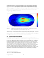
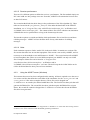
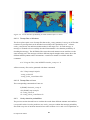
accuracy of 0.1nT from 2000 and onwards. CODE2 produces global Total Electron Content
(TEC) maps every second hour. Figure 2.1 shows a contour plot of such a map at 12:00 UTC on
July 1 2005. The TEC-value used to estimate Faraday rotation is calculated by linear interpolation
between successive maps at the relevant time. These calculations include the rotation of the
ionosphere maps with respect to the Earth.
Figure 2.1 CODE produces global TEC maps every second hour. The figure above shows a
contour plot of such a map at 12:00 UTC on July 1 2005.
AISDET requires a satellite antenna pattern to compute the received signal strengths. The pattern
can be selected from a set of ideal patterns or loaded from a file that describes the antenna pattern
including polarization. Section 4.2.2.4 describes the antenna setup in detail.
2.2
Performance Assessment Method
The SOTDMA protocol is designed to avoid transmissions of messages in the same slot for
vessels within each other’s field of view. A satellite will receive multiple messages transmitted at
the same time if there are more than a few hundred vessels within its field of view. Furthermore,
messages transmitted in adjacent slots may interfere due to differences in travel times. Each
interfering message has a specific Doppler shift, which varies between ±4kHz. The interference
from a message with a relative Doppler shift of 4 kHz is less than the interference from an
identical message with no relative Doppler shift. AISDET takes into account this effect either by
integrating over the overlapping spectrums to determine the interference level, or by using
receiver performance lookup tables. Differences in travel times cause messages to partly overlap,
which implies a bit error rate that varies during the message. The probability of decoding a
message is
2
http://www.cx.unibe.ch/aiub/ionosphere.html
FFI-rapport 2011/02300
7
224
P   (1  pi )
i 1
(2.1)
pi is the bit-specific bit error rate for signal to interference or signal to noise. The interference is
treated as white noise if there are no suitable look-up tables for the receiver performance with one
or more interfering sources. Each message’s detection probability is written to a file. This
assumes that 224 bits are necessary to successfully decode a message. Messages of type 1, which
is the most common transmitted message, have 168 bits plus an additional 16 bits for CRC check.
Hence, the 224 bits include training sequence start flag etc.
The performance of the system is determined by either counting the number of ships flagged as
detected within target areas or by analyzing files with message probabilities.
2.3
Input / Output Data
Figure 2.2 gives an overview of the inputs to and outputs from the simulation software. Required
inputs:






Orbital elements of the satellites
AIS payload antenna pattern, either an ideal pattern or a numerical model
A numerical model should include the effect of the platform on the pattern
Antenna orientation in space, nadir pointing antenna or offset from nadir
Ionosphere map, if the antenna is not circular polarized
Receiver performance, which can be estimated either from a performance lookup-tables
or by selecting the required signal to noise for 20% packet error rate. The first option
must include performance as a function of signal to noise and optionally the performance
as a function of the number of interfering messages and the Doppler shifts of the
interfering messages. The second option uses an approximate function to estimate the bit
error rates at other levels.
o The algorithm may be iterative, i.e. it attempts to remove decoded messages from
the received signal to see if other messages can be decoded.
Locations of ground stations can optionally be used to compute the timeliness of the data and
estimated data storage requirements.
The outputs are:




Files that provides the coordinates of the sub-satellite point, the number of vessels within
the field of view, the number of detected vessels and statistics of the number of messages
per slot every 10 second.
Files with the detection probability of each message
Vessel detection probability maps (per orbit and accumulated maps)
Detection times of each vessel. These files can be loaded by Satellite Toolkit (STK) to
create multi-track objects.
8
FFI-rapport 2011/02300
Figure 2.2 The inputs to and outputs from AISDET
3
Installation
The AISDET software collection requires a couple of external programs that compute satellite
orbits and access times to ground stations and target areas. These programs are included in the
Heliosat installer.
3.1
3.1.1
Windows
Installing Heliosat
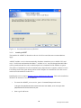
Heliosat is distributed as an ordinary Windows installer, Heliosat-1.0.1-win32.exe. It is strongly
recommended to keep the default settings, which includes installing to the path shown in Figure
2.1 even on a 32-bit OS. AISDET includes some scripts and programs that assume C:\Program
Files (x86) as an installation prefix. The installer will create a shortcut to remove Heliosat from
the system under Start All Programs.
FFI-rapport 2011/02300
9
Figure 3.1 Recommended location of Heliosat
3.1.2
Installing AISDET
The installer for AISDET is identical to the one for Heliosat and the same recommendations
apply.
AISDET includes a service that automatically distributes simulations over available CPUs and
cores. It will create and monitor the folder C:\\AISSim\\server. Any file dropped into this folder
will be parsed and each line with a valid description of a simulation will be added to its queue.
The number of simulations it will run simultaneously depends on the computer’s number of cores.
It will keep track of the queue during reboots of the computer it is installed on. How this service
can be used is described in section 4.2.3.
Installing this service requires Windows Server 2003 Resource Kit Tools. This can be installed on
Windows XP and newer version of Windows.
1.
To create the AISDET_server service, open a Command Prompt and execute:
"C:\Program Files (x86)\Windows Resource Kits\Tools\instsrv.exe" AISDET_server "C:\Program Files
(x86)\Windows Resource Kits\Tools\srvany.exe"
2.
Start regedit and locate
10
FFI-rapport 2011/02300
HKEY_LOCAL_MACHINE\SYSTEM\CurrentControlSet\Services\AISDET_server
1. From the Edit menu, click New  Key and rename it to Parameters
2. Select the Parameters key.
3. From the Edit menu, click New  String Value, rename it to Application and select
Modify from the Edit menu. Set Value Data to
C:\Program Files (x86)\AISDET\bin\aisdet_server.exe
4. Close Registry Editor.
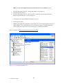
5. Start the compmgmt.msc using Start  Run. Select Service and Applications  Services,
locate AISDET_server and start the service as shown in Figure 3.2. Right click on the
service and select Properties to set its start-up type. It should be Automatic.
This is a summary of http://support.microsoft.com/kb/137890.
Figure 3.2 Starting the AISDET server
FFI-rapport 2011/02300
11
3.1.3
Windows PowerShell
It is necessary to have Windows PowerShell installed with a policy that allows it to run unsigned
scripts. It should be sufficient to execute
Set-ExecutionPolicy "RemoteSigned"
in a PowerShell terminal.
3.2
Linux
The Linux version also includes scripts to help running the simulations. These scripts assume that
Heliosat and AISDET have been installed to the user home directory. Installing Heliosat and
AISDET therefore amounts to running the following commands from a terminal
sh Heliosat-1.0.1-Linux.sh --prefix=${HOME}
sh AISDET-1.0.1-Linux.sh --prefix=${HOME}
It is necessary to accept the license agreement and not include subdirectories. This version does
not come with a server since atd combined with included scripts performs many of the same
tasks. atd is included with most Linux distributions and must be configured according to your
system specifications.
4
End to End performance analysis
The first step is to create a catalog structure. Each satellite must reside in its own folder, and it is
strongly recommended to give each folder a name that consists of two digits. For a 12 satellite
constellation with three satellites in each plane, the folder names could be 11, 12, 13, 21, 22, 23,
31, 32, 33, 41, 42 and 43.
Two examples have been included with the software. They can be found in
C:\Program Files (x86)\AISDET\share\aisdet\examples on Windows and in
${HOME}/share/aisdet/examples on Linux. The following walkthrough assumes that the
examples folder has been copied to C:/Temp on Windows and ${HOME}/tmp on Linux.
4.1
Propagate orbits
The first step of any simulation is to propagate an orbit for each satellite in the constellation. The
orbit propagator is a console program that must be run once for each satellite. It should be run
within each satellite folder, i.e. inside 11, 12…
12
FFI-rapport 2011/02300
4.1.1
Windows
The propagator is a console program. To see its user manual, start Windows PowerShell and
execute:
& 'C:\Program Files (x86)\Heliosat\bin\odesolver.exe' -h
This software is quite complicated to run correctly. The examples folder contains for each
satellite odesolver.bat, which simplifies this set. The following commands will generate the
necessary orbits.
cd C:\Temp\examples\dipoles\11
.\run_odesolver.bat
mv heliosat*orb satellite11.orb
cd C:\Temp\examples\dipoles\12
.\run_odesolver.bat
mv heliosat*orb satellite12.orb
cd C:\Temp\examples\ patch_arrays\11
.\run_odesolver.bat
mv heliosat*orb satellite11.orb
cd C:\Temp\examples\ patch_arrays\12
.\run_odesolver.bat
mv heliosat*orb satellite12.orb
It should be sufficient to edit the epoch, start time, stop time and the satellite file in the bat-script
for other scenarios. The examples include necessary satellite files, and in these files it is sufficient
to edit the lines with Orbital elements and initial conditions.
It is quicker to use tlesolver.exe if there are TLEs for each satellite, and it too has a user manual
available with the –h switch. odesolver.exe is quite slow as it is currently designed to propagate
orbits for a month with cm accuracy.
4.1.2
Linux
On Linux the corresponding commands are:
${HOME}/bin/odesolver -h
cd ${HOME}/tmp/examples/dipoles/11
sh ./run_odesolver.sh
mv heliosat*orb satellite11.orb
FFI-rapport 2011/02300
13
cd ${HOME}/tmp/examples/dipoles/12
sh ./run_odesolver.sh
mv heliosat*orb satellite12.orb
cd ${HOME}/tmp/examples/patch_arrays/11
sh ./run_odesolver.sh
mv heliosat*orb satellite11.orb
cd ${HOME}/tmp/examples/patch_arrays/12
sh ./run_odesolver.sh
mv heliosat*orb satellite12.orb
4.2
Running the simulations
The aisdet program is an end to end simulation tool for reception of AIS messages in space.
Running the program without any arguments will write a simple user manual to the console:
"C:\Program Files (x86)\AISDET\bin\aisdet.exe"
This program takes from one to three arguments. The first argument is a text file that acts as a
configuration file. Only an overview of this file will be given in this section, since the
configuration files included with the examples contain their own documentation. The second
argument determines how long to run a simulation. The last argument is used to set the
polarization of specific antenna patterns, see section 4.2.2.4.
It is necessary to create sub-folders for each AIS antenna, since each antenna (pattern) requires
one simulation. For example C:\Temp\examples\dipoles\11 has X, Y, and Z folders for three
different antennas with one configuration file in each folder. The examples can be run without
any modifications.
4.2.1
The init file
The contents of the init file must be in the same order as they are in the examples. This section
will not describe the entire file since the files included with the examples are heavily commented.
4.2.2
Data storage
The first section describes where AISDET shall look for vessel traffic models, antenna patterns
and required input files.
# Lines that start with a “#” are treated as comments
PATHS
Vessel data
: C:\Program Files (x86)\AISDET\share\aisdet\vessel_data
Antennas
: C:\Program Files (x86)\AISDET\share\aisdet\antennas
Input files
: C:\Program Files (x86)\AISDET\share\aisdet\input_files
14
FFI-rapport 2011/02300
4.2.2.1 Orbit
The second section tells AISDET to load an ephemeris file.
# The orbit file contains the ephemeris and required epochs.
ORBIT
Ephemeris
: ..\satellite11.orb
4.2.2.2 Vessel list
The vessel list files contain for each vessel: latitude, longitude, distance (km) to nearest coastline,
messages per minute and nominal transmission interval in slots. The software comes with several
vessel distributions for class A and class B equipped vessels. AISDET assumes that class B
vessels transmit at 2W.
# Load vessel data
VESSELS CLASS A
Vessel file
: vessel_list_espais2014.list
VESSELS CLASS B
Vessel file
: none
# Some suggestions for third (and fourth) frequencies require that only
# vessels without access to any land based base station should transmit
# on these frequencies. Setting the following value to true removes all
# vessels that are less than 40nm from any coast
COAST
Delete vessels near
: false
4.2.2.3 Coverage and SOTDMA files
This section is only important if the intent is to simulate more than one antenna on a satellite.
AISDET cannot simulate multiple antennas in a single run, but multiple antennas can be achieved
by running one simulation for each antenna and combining the results for all antennas in a post
processing step. This requires that each run uses exactly the same message pool, which is the
purpose of the SOTDMA files. A SOTDMA files contains a list of message transmission times
for each vessel, and it can be generated as part of a simulation.
AIDET can also generate coverage files. They contain information about when the vessels are
visible from the satellite. It is always recommended to generate coverage files, since they are used
in the post processing step, and since it will speed up the runs for the other antennas.
# A file that contains the coverage for every vessel. Setting the output
# file to something different than none, tells aisdet to write a
# coverage file with the given name.
#
# Both values can be set to none
COVRGE
Coverage file
: none
Output file
: ..\satellite11.cov
# A predefined file with SOTDMA slots must be loaded when simulating
# multiple antennas to ensure identical transmissions for each slot.
#
FFI-rapport 2011/02300
15
# Setting the output file to something different than none, tells aisdet
# to write a SOTDMA file with the given name.
#
# Both values can be set to none
SOTDMA
SOTDMA file
: none
Output file
: ..\satellite11.sotdma
In order to run both examples, it is therefore necessary to first execute
& 'C:\Program Files (x86)\AISDET\bin\aisdet.exe' h_win.init 86400
in
C:\Temp\examples\dipoles\11\X
C:\ Temp\examples\dipoles\12\X
C:\ Temp\examples\patch_arrays\11\patch_07_0_0_0_0_PX
and
C:\ Temp\examples\patch_arrays\12\patch_07_0_0_0_0_PX
The other simulations can be started as soon at the SOTDMA files have been generated. These
simulations will load the relevant SOTDMA and coverage files.
4.2.2.4 Selecting an antenna
AISDET can load three different types of numerical antenna patterns in addition to several ideal
antenna patterns.
The first valid numerical antenna pattern is a slightly modified NEC–Win3 output (NOU) file.
These files require an additional header and one line consisting of dashes only. Examples of valid
files can be found in the data directory of your AISDET installation.
The second type of numerical antenna patterns are files produced by Thales Alenia Space (TAS)
as a part of [2]. These files can contain circular or linear polarized patterns; see
“patch_D_0.7_P_0_0_0_0.txt” and “patch_polar_D_0.6_P_0_0_0_0” respectively for examples.
The linear polarized patterns do not contain all the necessary information about the polarization.
This is the reason for the third argument to AISDET.
The final type of numerical antenna pattern requires two filenames on the antenna diagram line in
the init file. The first file must contain the “theta”-direction of the polarization and the second file
must contain the “phi” – direction. See for example “AIS_TET_3mon_P1_abs_Dir_Theta.csv”
and “AIS_TET_3mon_P1_abs_Dir_Phi.csv”.
3
C:\Program Files (x86)\AISDET\data\antennas
16
FFI-rapport 2011/02300
4.2.2.5 Receiver performance
There are five different options to define the receiver’s performance. The first method simply sets
D/U ratio in dB at a 20% package error rate. From this, AISDET will estimate the bit error rates
at other D/U rations.
The second method loads the tables that give the performance of the ESA algorithm [2]. These
tables are located in the “perf_detector_*interf.txt” files under the data folder of the AISDET
installation, see “C:\Program Files (x86)\ AISDET\share\aisdet\input_files” on Windows and
“${HOME}/share\aisdet\input_files.” The content of these files can be edited to run simulations
with different receiver performances as long as the format stays the same.
The last three options are similar and define which performance files to load for two and three
colliding messages. AISDET will use the ESA tables for any other number of colliding
messages.
4.2.2.6 Other
Each simulation expects to find a “media” file in the work folder. It contains two sections: The
first section describes how to treat the troposphere. This section is not used by AISDET, and it is
necessary to set the method to zero and filename to “NONE”. The second section tells AISDET
to load ionosphere data. There are several different options, but AISDET can only use CODE
files. Examples of data files can be found in “C:\Program Files
(x86)\Heliosat\share\Heliosat\ionosphere” on Windows and in
“${HOME}/share/Heliosat/ionosphere” on Linux. The shell script in the CODE folder can be
used to download data for other years on Linux machines.
4.2.3
Using the AISDET server (Windows)
This assumes that server has been configured and is running. All that is required to use the server
is to create text files that define the work folder of the simulation. See the “server_part1.txt” and
“server_part2.txt” files in the examples directory. These files can be dropped into
C:/AISSim/server to start the jobs defined within these files. The first file lists those jobs that will
generate SOTDMA files. The second file lists those jobs that require SOTDMA files as input.
Hence, the second file cannot be dropped into C:/AISSim/server before the relevant SOTDMA
files have been generated4.
4
This is not strictly true. Both files can be dropped into C:/AISSim/server at the same time as long as there
are fewer cores on the workstation than SOTDMA generating simulations.
FFI-rapport 2011/02300
17
It is strongly recommended to check that the simulations are correctly configured before they are
sent to the server. This can be achieved by running the simulation over a short time in Windows
PowerShell:
& 'C:\Program Files (x86)\AISDET\bin\aisdet.exe' h_win.init 100
4.2.4
Using atd (Linux)
The shell scripts batch_part1.jobs and batch_part2.jobs use atd to achieve the same service on
Linux as the AIDET server on Windows.
4.3
Modifying the receiver performance
The best way to modify the receiver performance is to edit the location of the input files in the
configuration file for AISDET, and the copy the original contents to the new location. There are
three (sets of) files that can be edited.
The file “filter.txt” contains the filter characteristics for the receiver. Its first column gives the
relative frequency offset in kHz for messages arriving at the same time, while its second column
gives discrimination in dB. Hence, this file tells AISDET how to correct the received signal
strength of a colliding message with a given frequency offset to the message its attempting to
decode. The number of frequency steps is not important, but it must be in increasing order.
It is also possible to change the performance of the SIC algorithm if SIC is set in the AISDET
configuration file. The performance of the algorithm is defined in the file “sic.txt”. Its first
column gives D/U, i.e. signal strength of the desired signal to the undesired signal(s). The second
column set how much of the desired signal that can be removed if the message has been
successfully decoded. The first or the last value will be used if the D/U is out of bounds.
The last files are the “perf_detector_*interf.txt” files, which gives the performance for 0, 1, 2 or 5
colliding messages. The first column in these files gives the Signal to Noise Ratio (SNR) for the
received messages. The next columns give the Bit Error Rates for different C/I values.
4.4
Post processing
The post processing is done using software included with the Heliosat and AIDET packages. All
the programs are driven from the command line, but some of the programs are nearly impossible
to set up manually due to large number of arguments. The AISDET installation comes with
several scripts that do most of the heavy lifting. These scripts can also be found in the folder with
the examples, and those scripts can be used without any modifications. However, other
simulations might require some editing in a text editor. Hopefully, the comments in the scripts
should be sufficient to understand what the different settings do. Only the dipole example will be
covered in this section. The post processing steps for the patch arrays are for all purposes
identical.
18
FFI-rapport 2011/02300
4.4.1
Plotting detection probabilities per antenna
Each simulation produces a set of files named “ais_accprob_orbXXX.dat” and
“ais_accprob_orbXXX.dat”. These files contain respectively a map of the detection probabilities
for orbit number XXX and the detection probability for orbits up to and including number XXX.
The data folder of the AISDET installation contains MatLab scripts to plot these maps. This
folder must be in MatLab’s search path and MatLab must have the Mapping Toolbox installed.
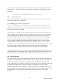
The MatLab command to plot detection probabilities for a single antenna is:
plotprob_folder(‘C:\Temp\examples\dipoles\12\X',0,1,15,0,0,'Satellite 12, X - antenna, orbit 000')
This command plots orbit number 1 through 15, and the script contains an explanation of the
arguments. Figure 4.1 gives an example of a resulting probability map. Plotting accumulated
detection probability maps is similarly:
plotprob_folder(‘C:\Temp\examples\dipoles\12\X',1,1,15,0,0,'Satellite 12, X - antenna, orbit 000')
Figure 4.2 shows the accumulated detection probability after 15 orbits for a single antenna.
Figure 4.1 Detection probability over one orbit for a single antenna
FFI-rapport 2011/02300
19
Figure 4.2 Detection probability accumulated over 15 orbits
4.4.2
Detection probabilities for each orbit
The previous figures show only the results for a single antenna. It is possible to combine the
results from different antennas and satellites into single maps. This requires a set of remap files
that can be generated with the help the program called aisdet_remap. Section 4.4.2.1 and 4.4.2.2
describes how to generate the necessary files on Windows and Linux. The following command
plots the total detection probability of one satellite:
plotprob_folder(‘C:\Temp\examples\dipoles \11',0,1,15,1,0,'Single satellite, orbit 000')
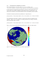
It is also possible to plot the accumulated detection probability over 15 orbits using both
satellites:
plotprob_folder(‘C:\Temp\examples\dipoles',1,1,15,1,0,'Both satellites, orbit 000')
These maps contain detection probabilities for those 1x1 degree cells that contain at least one
vessel, see Figure 4.3 and Figure 4.4.
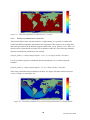
Figure 4.3 Detection probability over one orbit using all antennas on a single satellite
20
FFI-rapport 2011/02300
Figure 4.4 Final detection probability for both satellites after 15 orbits
4.4.2.1 Remap files on Windows
The above plots require a set of remap files that aisdet_remap generates. It uses a set of files that
contain every message that can be decoded successfully with a probability of 10-7 or better.
aisdet_remap draws one uniform random number in the range 0 to 1 for each message. A
message is assumed to be successfully decoded if that number is less than the probability of
decoding the message. The SOTDMA files ensure that each antenna on one satellite sees the
same message pool. The messages will have different signal strengths at the sensor due to the
different antenna patterns and/or orientations. A small user manual is available with this
command:
& 'C:\Program Files (x86)\AISDET\bin\aisdet_remap.exe' -h
All the necessary files can be generated with these commands
cd C:\Temp\examples\dipoles
.\remap_orbits.PS1
.\remap_orbits_constellation.PS1
4.4.2.2 Remap files on Linux
The corresponding commands on Linux are
${HOME}/bin/aisdet_remap -h
cd ${HOME}/tmp/examples
sh ./remap_orbits.sh
sh ./remap_orbits_constellation.sh
4.4.3
Hourly detection probabilities
The previous section showed how to combine the results from different antennas and satellites
over specific orbits. It is also possible to use aisdet_remap to combine the message probability
files with a step size of one hour instead of one orbit. Sections 4.4.3.1 and 4.4.3.2 explain how to
FFI-rapport 2011/02300
21
do this. The following two commands correspond to the two MatLab commands in the previous
section:
plotprob_folder(‘C:\Temp\examples\dipoles \11\hours_01_06',0,1,6,1,1,'One satellite, hour 000')
plotprob_folder(‘C:\Temp\examples\dipoles\hours_01_06',1,1,6,1,1,'Both satellites, orbit 000')
Figure 4.5 Detection probability for a single satellite after one hour
Figure 4.6 Detection probability for both satellites after the first 6 hours
4.4.3.1 Hourly remap files on Windows
The hourly remap files might take a lot longer to create using the included scripts. These scripts
contain a variable called DELTA, which has been set to 6 (hours). The script will start with hours
1 through 6, and it will for each hour create both single hour detection probability maps and
accumulated detection probability maps. The script will redo the same process on hours 2 through
7 and so on until the end of the simulations. Hence, DELTA can be interpreted as the length of a
moving window where the scripts create detection probability maps. The commands are:
cd C:\Temp\examples\dipoles
.\remap_hours.PS1
.\remap_hours_constellation.PS1
22
FFI-rapport 2011/02300
4.4.3.2 Hourly remap files on Linux
cd ${HOME}/tmp/examples
sh ./remap_ hours.sh
sh ./remap_ hours_constellation.sh
4.4.4
Table of detection probabilities in target areas
aiscnt is a program that counts the number of vessels within a target area and how many of those
vessels that were detected within a user selected interval. The following commands will generate
a simple table of detection probabilities:
Linux:
cd ${HOME}/tmp/examples
sh aiscnt.sh
Windows:
cd C:\Temp\examples\dipoles
.\aiscnt.PS1
4.4.5
Global map of update intervals
The purpose of this section is to produce a global map that show how much time it takes to
receive updates from 80% of the vessels. It requires access times for each satellite to a set of user
selected ground stations. These access times can be generated using the program access that is
included with the Heliosat package. To see a simple user manual, execute:
& 'C:\Program Files (x86)\Heliosat\bin\access.exe' –h
access requires ground stations listed in a text file that has a specific format. The examples
include ground station files that define two ground stations, one in Madrid and the other in
Cyprus. To compute access times on Linux:
cd ${HOME}/tmp/examples/dipoles/11
access -o satellite11.orb -g ground_stations.stat -r satellite11.acss
cd ${HOME}/tmp/examples/dipoles/12
access -o satellite12.orb -g ground_stations.stat -r satellite12.acss
Windows:
cd C:\Temp\examples\dipoles\11
& 'C:\Program Files (x86)\Heliosat\bin\access.exe' -o satellite11.orb –g
FFI-rapport 2011/02300
23
ground_stations.stat -r satellite11.acss
cd C:\Temp\examples\dipoles\12
& 'C:\Program Files (x86)\Heliosat\bin\access.exe' -o satellite12.orb –g
ground_stations.stat -r satellite12.acss
Keep these access files as they will be needed in the next sections too.
The global map can now be created with help of scripts included with the examples. These scripts
use the program aiscnt_dist:
Linux:
sh aiscnt_map.sh
Windows:
.\aiscnt_map.PS1
A small warning is needed here. These scripts and the scripts in the next section add one
argument, -iup, to the aiscnt_dist list of arguments. It causes aiscnt_dist to ignore update intervals
longer than 256 minutes because of the constellation's coverage. This option will have little or no
effect on large constellations. The resulting files can again be plotted with the help of a MatLab
script included with AISDET:
plotprob_func(1, 'Dipoles', ‘C:\Temp\examples\dipoles\map_update_interval.dat', '', 1,1)
This will generate a figure that you have to save manually. It might be a good idea to edit the
color map before the figure is saved, since the color maps defaults to a maximum value of 24
hours. Figure 4.7 illustrates such a map after setting the maximum value in the color map to 6
hours.
24
FFI-rapport 2011/02300
Figure 4.7 Required time to get updates from 80% of the vessel. Dark red implies an update
interval of six hours or more. This map ignores the times when an area can not been
seen due the two satellites coverage.
4.4.6
Distribution of update intervals
aiscnt_dist can also generate distributions of update intervals within selected target areas. A set of
scripts included with the examples simplifies this process:
Linux:
cd ${HOME}/tmp/examples/dipoles
sh aiscnt_dist.sh
Windows:
cd C:\Temp\examples\dipoles
.\aiscnt_dist.PS1
The output will be a large set of text files and four figures for each target area. Both of these
scripts require that gnuplot is installed and in the system’s path variable.
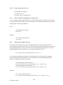
The first figure gives the fraction of vessels inside a target area that the users can expect to
receive updates from within a given time interval assuming a set of ground stations. Figure 4.8 is
an example of such a figure. It also includes curves for vessels with specific repetition intervals
and for vessels on open seas. This figure is based on a common distribution of update intervals
for all of the vessels within the target area. The plateau at the right end of the figure indicates the
detection probability within this target area. Figure 4.9 is an example of the second type of
figures. It gives the distribution of mean update intervals for the vessels within a target area.
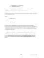
Figure 4.10 and Figure 4.11 correspond to Figure 4.8 and Figure 4.9, but show instead the time it
takes to get the data to the users. These last two figures are scaled to the fraction of the detected
vessels instead of the fraction of all of the vessels within the target area. Figures like Figure 4.8
might in some cases show vessels with update intervals close to zero minutes. This happens if a
FFI-rapport 2011/02300
25
vessel is seen by satellites over multiple passes without access to a ground station. It is therefore
important that the timeliness is shorter than the revisit time of a target area.
Figure 4.8 The fraction of vessels in the North Atlantic that the users can expect to receive
updates from within a given time interval assuming ground stations in Cyprus and
Madrid
26
FFI-rapport 2011/02300
Figure 4.9 Fraction of vessels as a function of the vessels’ mean update interval in the North
Atlantic assuming ground stations in Cyprus and Madrid
Figure 4.10 The fraction of detected vessels in the North Atlantic as function of the time it takes
to get the data to the user assuming ground stations in Cyprus and Madrid
FFI-rapport 2011/02300
27
Figure 4.11 Fraction of detected vessels as a function of the average time it takes to get data to
the ground assuming ground stations in Cyprus and Madrid
There is also a small script to summarize the results from the above analysis. The following
commands on Linux and Windows produce a small table that shows how many vessels the users
can expect to get updates from within 60 and 180 minutes.
Linux:
cd ${HOME}/tmp/examples/dipoles
mkdir update_timeliness_02_groundstations
mv update_interval_* update_timeliness_02_groundstations/
mv timeliness_* update_timeliness_02_groundstations/
mv cdfu* update_timeliness_02_groundstations/
mv cdft_* update_timeliness_02_groundstations/
sh summarize_update_intervals.sh update_timeliness_02_groundstations
28
FFI-rapport 2011/02300
Windows:
cd C:\Temp\examples\dipoles
.\aiscnt_dist.PS1
mkdir update_timeliness_02_groundstations
mv update_interval_* update_timeliness_02_groundstations/
mv timeliness_* update_timeliness_02_groundstations/
mv cdfu* update_timeliness_02_groundstations/
mv cdft_* update_timeliness_02_groundstations/
.\summarize_update_intervals.PS1
4.4.7
Detection probability in a moving window
The last scripts are used to compute detection probabilities within moving windows. The length
of the windows and the target areas are set in the script. These scripts output text files, which
contain one line for each time step. The first column is the middle of the interval, then follows the
number of detected vessels, the number of vessel inside the target area, time, latitude and
longitude of the last detected vessel, and finally the fraction of detected vessels.
The scripts in the examples give results for a single satellite. However, it should be trivial to edit
the scripts to show results for two satellites.
Linux:
cd ${HOME}/tmp/examples/dipoles
sh aiscnt_intervals.sh
gnuplot plot_interval.gp
Windows (may warn about files that do not exist):
cd C:\Temp\examples\dipoles
.\aiscnt_intervals.PS1
& 'C:\Program Files (x86)\gnuplot\binary\gnuplot.exe' plot_interval.gp
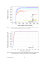
Figure 4.12 shows the output from the above two commands.
FFI-rapport 2011/02300
29
Figure 4.12 Detection probabilities in different target areas using a three hour moving window
4.5
Post processing without AISDET
It is possible to do two of the post-processing steps, see section 4.4.5 and 4.4.6, without running
AISDET first. This requires one file that list the MMSI, latitude and longitude of each vessel and a
set of files that lists reception and ground times for each decoded message. A typical run would
look something like the following
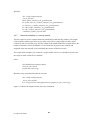
& 'C:\Program Files (x86)\AISDET\bin\aiscnt_dist.exe' –s vessels.txt
-d messages_sat1.txt messages_sat2.txt messages_sat3.txt
-p poygon_north_atlantic.plg
The “vessels.txt” must contain one line per vessels, and each line must be on the form:
MMSI latitude longitude
The “messages_sat*.txt” files list every successfully decoded message. Each file must begin with
a common epoch header and then one line per message:
2005-07-01 12:00:00.00
555533221 01 JUL 2005 21:10:40.000 01 JUL 2005 23:00:12.234
444422111 01 JUL 2005 19:31:00.000 01 JUL 2005 20:45:01.000
444422111 01 JUL 2005 21:09:50.000 01 JUL 2005 22:21:12.000
The first column is the MMSI, which is followed by reception and ground time.
30
FFI-rapport 2011/02300
To see a simple user manual for aiscnt_dist, execute
& 'C:\Program Files (x86)\AISDET\bin\aiscnt_dist.exe' -h
5
Summary
This software has been tested comprehensively, but some bugs might still have gone by
unnoticed, and the packaging process might have introduced problems with missing files and or
wrong files. Any questions or bug reports may be sent to [email protected]. New features will
not be added unless it is required by the work done at FFI, or unless it is required by projects that
FFI participates in.
References
[1] Øystein Olsen, "ESPAIS AIS System Study - Maritime Traffic Characterization," 2010.
[2] Øystein Olsen, "ESPAIS AIS System Study - Payload Performance Analysis Report,"
2010.
FFI-rapport 2011/02300
31