Download PPMS TTO Manual - Materials Research Laboratory at UCSB

Physical Property
Measurement System
Thermal Transport Option User’s Manual
Part Number 1684-100B
Quantum Design
11578 Sorrento Valley Rd.
San Diego, CA 92121-1311
USA
Technical support
(858) 481-4400
(800) 289-6996
Fax
(858) 481-7410
Third edition of manual completed October 2002.
Trademarks
All product and company names appearing in this manual are trademarks or registered trademarks of their respective holders.
U.S. Patents
4,791,788 Method for Obtaining Improved Temperature Regulation When Using Liquid Helium Cooling
4,848,093 Apparatus and Method for Regulating Temperature in a Cryogenic Test Chamber
5,311,125 Magnetic Property Characterization System Employing a Single Sensing Coil Arrangement to Measure AC
Susceptibility and DC Moment of a Sample (patent licensed from Lakeshore)
5,647,228 Apparatus and Method for Regulating Temperature in Cryogenic Test Chamber
5,798,641 Torque Magnetometer Utilizing Integrated Piezoresistive Levers
Foreign Patents
U.K.
9713380.5 Apparatus and Method for Regulating Temperature in Cryogenic Test Chamber
C
O
N
T
E
N
T
S
Table of Contents
PREFACE ..............................................................................................................................................................vii
Contents and Conventions ...............................................................................................................................vii
P.1
P.2
P.3
P.4
Introduction ......................................................................................................................................................vii
Scope of the Manual.........................................................................................................................................vii
Contents of the Manual ....................................................................................................................................vii
Conventions in the Manual..............................................................................................................................viii
CHAPTER 1
Introduction ......................................................................................................................................................... 1-1
1.1 Introduction .................................................................................................................................................... 1-1
1.2 Overview of the Thermal Transport Option ................................................................................................... 1-1
1.2.1 Purpose of Measuring Thermal Transport Properties .............................................................................. 1-3
1.3 Measurement Modes....................................................................................................................................... 1-3
1.3.1 Continuous Measurement Mode .............................................................................................................. 1-3
1.3.2 Single Measurement Mode ...................................................................................................................... 1-3
1.4 Measured Thermal Properties......................................................................................................................... 1-5
1.4.1 Thermal Conductivity .............................................................................................................................. 1-5
1.4.2 Seebeck Coefficient ................................................................................................................................. 1-5
1.4.3 Electrical Resistivity ................................................................................................................................ 1-6
1.4.4 Figure of Merit......................................................................................................................................... 1-6
1.5 Theory of Operation ....................................................................................................................................... 1-7
1.5.1 Hardware ................................................................................................................................................. 1-7
1.5.2 Thermal and Electrical Circuit................................................................................................................. 1-7
1.5.3 Software Models...................................................................................................................................... 1-8
1.5.4 Estimating Errors in the Data................................................................................................................... 1-9
1.5.5 Correcting for Heat Loss........................................................................................................................ 1-11
1.5.6 Correcting for Seebeck Coefficient of Manganin Leads........................................................................ 1-11
1.6 Start-up Checklist for Secondary Installation ............................................................................................... 1-11
CHAPTER 2
Hardware .............................................................................................................................................................. 2-1
2.1 Introduction .................................................................................................................................................... 2-1
2.2 Thermal Transport Hardware.......................................................................................................................... 2-1
2.2.1 Thermal Transport Sample Puck ............................................................................................................. 2-2
2.2.2 User’s Kit................................................................................................................................................. 2-3
2.2.3 Nickel Calibration Samples ..................................................................................................................... 2-5
2.2.4 WaveROM EPROM ................................................................................................................................ 2-5
2.2.4.1 Replacing the WaveROM Chip ........................................................................................................ 2-6
2.2.5 Thermal Transport Connection Cable...................................................................................................... 2-6
2.2.6 User Bridge Board ................................................................................................................................... 2-7
2.3 ACT Hardware ............................................................................................................................................... 2-7
2.3.1 Model 7100 AC Transport Controller...................................................................................................... 2-7
2.3.2 AC Board................................................................................................................................................. 2-7
Quantum Design
PPMS Thermal Transport Option User’s Manual
i
Contents
Table of Contents
2.4 High-Vacuum Hardware................................................................................................................................. 2-8
2.4.1 Contact Baffle.......................................................................................................................................... 2-8
2.5 Calibrating New Shoe Assemblies ................................................................................................................. 2-9
CHAPTER 3
Software ................................................................................................................................................................. 3-1
3.1 Introduction .................................................................................................................................................... 3-1
3.2 Overview of Thermal Transport Software ...................................................................................................... 3-1
3.2.1 Measurement Units.................................................................................................................................. 3-2
3.3 Thermal Transport Control Center ................................................................................................................. 3-3
3.3.1 Control Center Tabs................................................................................................................................. 3-3
3.3.2 Measurement Menu ................................................................................................................................. 3-5
3.3.2.1 Options for Advanced Users............................................................................................................. 3-8
3.3.3 System Status........................................................................................................................................... 3-9
3.4 Thermal Transport Data Files ....................................................................................................................... 3-10
3.4.1 Saving Raw Thermal Transport Data .................................................................................................... 3-10
3.4.2 Data File Header .................................................................................................................................... 3-10
3.4.3 Format of Measurement Data Files........................................................................................................ 3-11
3.4.4 Format of Raw Data Files...................................................................................................................... 3-13
3.5 Data Examination ......................................................................................................................................... 3-14
CHAPTER 4
Sample Preparation .......................................................................................................................................... 4-1
4.1 Introduction .................................................................................................................................................... 4-1
4.2 Sample-Mounting Considerations .................................................................................................................. 4-1
4.2.1 Geometry ................................................................................................................................................. 4-2
4.2.2 Lead-Mounting Epoxies .......................................................................................................................... 4-3
4.2.2.1 Silver-Filled H20E Epoxy ................................................................................................................ 4-3
4.2.2.2 Tra-Bond 816H01 Epoxy.................................................................................................................. 4-3
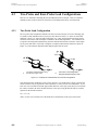
4.3 Two-Probe and Four-Probe Lead Configurations........................................................................................... 4-4
4.3.1 Two-Probe Lead Configuration ............................................................................................................... 4-4
4.3.2 Four-Probe Lead Configuration............................................................................................................... 4-5
4.4 Checking the Sample Contact......................................................................................................................... 4-6
4.5 Using the Puck-Mounting Station................................................................................................................... 4-6
CHAPTER 5
Measurements ..................................................................................................................................................... 5-1
5.1 Introduction .................................................................................................................................................... 5-1
5.2 Taking Thermal Transport Measurements...................................................................................................... 5-1
5.2.1 Connect Leads to the Sample................................................................................................................... 5-2
5.2.2 Measure the Sample Dimensions............................................................................................................. 5-2
5.2.3 Mount the Sample.................................................................................................................................... 5-3
5.2.4 Install the Sample .................................................................................................................................... 5-3
5.2.5 Start the High-Vacuum System ............................................................................................................... 5-3
5.2.6 Open the Data File ................................................................................................................................... 5-4
5.2.7 Define the Measurement.......................................................................................................................... 5-4
5.2.8 Run the Measurement .............................................................................................................................. 5-5
5.2.8.1 Running the Measurement Interactively ........................................................................................... 5-5
5.2.8.2 Running the Measurement in a Sequence ......................................................................................... 5-5
5.2.9 Scanning or Ramping the Temperature While Measuring....................................................................... 5-5
ii
PPMS Thermal Transport Option User’s Manual
Quantum Design
Contents
Table of Contents
5.3 Measurement Mode Parameters...................................................................................................................... 5-6
5.3.1 Continuous Measurement Mode .............................................................................................................. 5-6
5.3.2 Single Measurement Mode ...................................................................................................................... 5-8
5.4 Description of Measurement Process.............................................................................................................. 5-9
CHAPTER 6
Troubleshooting ................................................................................................................................................. 6-1
6.1 Introduction .................................................................................................................................................... 6-1
6.2 Jumps or Noise in the Data ............................................................................................................................. 6-1
6.2.1 Gaps in the Data Versus Temperature ..................................................................................................... 6-2
6.2.2 Steps in the Data ...................................................................................................................................... 6-2
6.3 Thermal Radiation “Tail” in the Thermal Conductivity Data......................................................................... 6-3
6.4 High-Vacuum Problems ................................................................................................................................. 6-3
CHAPTER 7
Maintenance ........................................................................................................................................................ 7-1
7.1 Introduction .................................................................................................................................................... 7-1
7.2 Using the Puck Adjustment Tool.................................................................................................................... 7-1
7.3 Greasing the Puck Fingers and the Coldfoot Clamp....................................................................................... 7-2
APPENDIX A
Installation............................................................................................................................................................A-1
A.1 Introduction................................................................................................................................................... A-1
A.2 Installing Thermal Transport Hardware........................................................................................................ A-1
A.3 Installing Thermal Transport Software ......................................................................................................... A-3
APPENDIX B
Status Codes and Error Messages ..............................................................................................................B-1
B.1 Introduction....................................................................................................................................................B-1
B.2 System Status Codes ......................................................................................................................................B-1
B.2.1 General PPMS System Status Codes ......................................................................................................B-1
B.2.2 Thermal Transport System Status Codes ................................................................................................B-3
APPENDIX C
Pinout Tables .......................................................................................................................................................C-1
C.1 Introduction....................................................................................................................................................C-1
C.2 Thermal Transport Pinouts.............................................................................................................................C-1
C.2.1 Sample Connections................................................................................................................................C-1
References ..............................................................................................................................................References-1
Index ................................................................................................................................................................ Index-1
Quantum Design
PPMS Thermal Transport Option User’s Manual
iii
Contents
Table of Figures
Figures
Figure 1-1. Thermal and Electrical Connections for an Idealized Sample ............................................................... 1-7
Figure 1-2. Heat Pulse and Temperature and Voltage Response at Hot and Cold Thermometer Shoes in an
Idealized Sample ........................................................................................................................... 1-8
Figure 2-1. TTO Puck with Radiation Shield ........................................................................................................... 2-2
Figure 2-2. Puck-Mounting Station with Puck ......................................................................................................... 2-3
Figure 2-3. Thermal Transport Option User’s Kit .................................................................................................... 2-4
Figure 2-4. WaveROM EPROM on AC Board in Model 6000 PPMS Controller ................................................... 2-5
Figure 2-5. Thermal Transport Connection Cable .................................................................................................... 2-6
Figure 2-6. Front Panel on Model 7100 AC Transport Controller ........................................................................... 2-7
Figure 2-7. Baffle Assembly with Contact Baffle .................................................................................................... 2-8
Figure 2-8. Close-up View of Contact Fingers and Charcoal Holder on Contact Baffle Assembly......................... 2-8
Figure 2-9. Calibration Fixture Plugged into TTO Puck and Illustrating Sockets for Each Shoe Assembly ......... 2-10
Figure 2-10. Thermal Transport Calibrate Thermometers and Heater Wizard....................................................... 2-10
Figure 3-1. Thermal Transport Log Window ........................................................................................................... 3-2
Figure 3-2. Control Center Install Tab...................................................................................................................... 3-3
Figure 3-3. Control Center Data File Tab................................................................................................................. 3-3
Figure 3-4. Control Center Sample Tab.................................................................................................................... 3-4
Figure 3-5. Control Center Waveform Tab............................................................................................................... 3-4
Figure 3-6. Control Center Advanced Tab ............................................................................................................... 3-5
Figure 3-7. Settings Tab in Thermal Transport Measurement Dialog Box .............................................................. 3-6
Figure 3-8. Thermal Tab in Thermal Transport Measurement Dialog Box.............................................................. 3-6
Figure 3-9. Resistivity Tab in Thermal Transport Measurement Dialog Box .......................................................... 3-7
Figure 3-10. Mode Tab in Thermal Transport Measurement Dialog Box ................................................................ 3-8
Figure 3-11. Advanced Tab in Thermal Transport Measurement Dialog Box ......................................................... 3-8
Figure 3-12. Error Count Dialog Box..................................................................................................................... 3-14
Figure 4-1. Examples of Leads Mounted in Two-Probe Configuration ................................................................... 4-4
Figure 4-2. Example of Leads Mounted in Four-Probe Configuration..................................................................... 4-5
Figure 5-1. Thermal Tab in Thermal Transport Measurement Dialog Box.............................................................. 5-6
Figure 5-2. Resistivity Tab in Thermal Transport Measurement Dialog Box .......................................................... 5-8
Figure 7-1. Puck Adjustment Tool ........................................................................................................................... 7-1
Figure A-1. Thermal Transport Option Connection Diagram ................................................................................. A-2
Figure C-1. Illustration of TTO Sample Connections, Showing Hardware Ports.....................................................C-2
Figure C-2. Top View of Pinout of Connector Sockets on Thermal Transport Sample Puck ..................................C-3
iv
PPMS Thermal Transport Option User’s Manual
Quantum Design
Contents
Table of Tables
Tables
Table 1-1.
Table 1-2.
Table 1-3.
Table 1-4.
System Requirements for the Thermal Transport System ....................................................................... 1-2
Thermal Transport System Parameters ................................................................................................... 1-2
Thermal Transport System Components ................................................................................................. 1-2
Styles for Measurements Taken in Single Measurement Mode .............................................................. 1-4
Table 2-1. Recommended Sample Parameters for Nickel Calibration Samples....................................................... 2-5
Table 3-1. PPMS System Data Items That Can Be Saved to the TTO Measurement Data File ............................... 3-9
Table 3-2. Fields in Thermal Transport Measurement Data File............................................................................ 3-11
Table 3-3. Fields in Thermal Transport Raw File................................................................................................... 3-13
Table 4-1. Sample Geometries and Range of Measurable Thermal Conductivities ................................................. 4-2
Table 4-2. Approximate Thermal Conductance of Epoxies...................................................................................... 4-5
Table 5-1. Minimum and Maximum Parameter Limits for Continuous Mode Measurements
5-6
Table 5-2. General Settings for Continuous Mode Measurements ........................................................................... 5-7
Table 5-3. Resistivity Excitation Parameters for Continuous Mode Measurements ................................................ 5-8
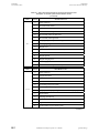
Table B-1. Status Associated with Bits of General System Status Field ..................................................................B-1
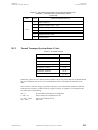
Table B-2. TTO Status Codes...................................................................................................................................B-3
Table C-1. TTO Sample Connections.......................................................................................................................C-2
Quantum Design
PPMS Thermal Transport Option User’s Manual
v
P
R
E
F
A
C
E
Contents and Conventions
P.1
Introduction
This preface contains the following information:
P.2
•
Section P.2 discusses the overall scope
of the manual.
•
Section P.3 briefly summarizes the
contents of the manual.
•
Section P.4 illustrates and describes
conventions that appear in the manual.
Scope of the Manual
This manual discusses the Thermal Transport option (TTO) for the Physical Property Measurement
System (PPMS). This manual explains how to use the TTO system and it explains the theory of
operation for TTO. This manual describes the hardware and software that are unique to TTO, and
it includes maintenance and troubleshooting information.
For detailed information about the PPMS MultiVu software, which is the parent software application
running the PPMS, refer to the Physical Property Measurement System: PPMS MultiVu Application
User’s Manual.
P.3
Contents of the Manual
•
Chapter 1 presents an overview of the
TTO system and of the TTO theory of
operation.
•
Chapter 5 explains how to take measurements with TTO and describes the
measurement process.
•
Chapter 2 discusses and illustrates the
hardware used with TTO.
•
Chapter 6 contains troubleshooting
suggestions.
•
Chapter 3 discusses the TTO software
and TTO data files.
•
Chapter 7 explains basic maintenance
procedures.
•
Chapter 4 explains how to prepare
samples for TTO measurements.
Quantum Design
PPMS Thermal Transport Option User’s Manual
vii
Section P.4
Conventions in the Manual
P.4
Preface
Contents and Conventions
•
Appendix A explains how to install the
TTO hardware and software.
•
Appendix B contains status codes and
error messages.
•
Appendix C contains pinout tables.
Conventions in the Manual
File menu
Bold text distinguishes the names of menus, options, buttons, and panels appearing
on the PC monitor or on the Model 6000 PPMS Controller LCD screen.
File¾Open
The ¾ symbol indicates that you select multiple, nested software options.
STATUS
Bold text and all CAPITAL letters distinguish the names of keys located on the front
panel of the Model 6000 PPMS Controller.
.dat
The Courier font distinguishes characters you enter from the PC keyboard or from
the Model 6000 PPMS Controller front panel. The Courier font also distinguishes
code and the names of files and directories.
<Enter>
Angle brackets < > distinguish the names of keys located on the PC keyboard.
<Alt+Enter>
A plus sign + connecting the names of two or more keys distinguishes keys you press
simultaneously.
A pointing hand and the word NOTE introduce a supplementary note.
NOTE
viii
CAUTION!
Cautionary notes are preceded with the word CAUTION! This signals conditions
that could result in loss of information or damage to your equipment.
WARNING!
Warnings are preceded with the word WARNING! This signals conditions that
could result in bodily harm or loss of life.
PPMS Thermal Transport Option User’s Manual
Quantum Design
C
H
A
P
T
E
R
1
Introduction
1.1
Introduction
This chapter contains the following information:
1.2
•
Section 1.2 presents an overview of
the TTO system.
•
Section 1.5 explains the TTO system’s
theory of operation.
•
Section 1.3 describes the TTO system
measurement modes.
•
Section 1.6 contains the start-up checklist
for secondary installation of the TTO.
•
Section 1.4 explains how the TTO
system measures thermal properties.
Overview of the Thermal Transport Option
The Quantum Design Thermal Transport option (TTO) for the Physical Property Measurement System
(PPMS) enables measurements of thermal properties, including thermal conductivity κ and Seebeck
coefficient (also called the thermopower) α, for sample materials over the entire temperature and
magnetic field range of the PPMS. The TTO system measures thermal conductivity, or the ability of a
material to conduct heat, by monitoring the temperature drop along the sample as a known amount of
heat passes through the sample. TTO measures the thermoelectric Seebeck effect as an electrical
voltage drop that accompanies a temperature drop across certain materials. The TTO system can
perform these two measurements simultaneously by monitoring both the temperature and voltage drop
across a sample as a heat pulse is applied to one end. The system can also measure electrical resistivity
ρ by using the standard four-probe resistivity provided by the PPMS AC Transport Measurement
System (ACT) option (Model P600). All three measurement types are essential in order to assess the
so-called “thermoelectric figure of merit,” ZT = α2T/κρ, which is the quantity of main interest if you
are investigating thermoelectric materials.
While the measurements taken with the TTO system are quite elementary in principle, they have
eluded commercialization because the data was typically very error prone, time consuming, and
laborious, due⎯for example⎯to problems in controlling heat flow and accurately measuring small
temperature differentials in a convenient manner. The TTO system has solved or greatly reduced
many of these experimental complications. TTO uses convenient sample mounting, small and highly
accurate Cernox chip thermometers, and sophisticated software that dynamically models an AC heat
flow through the sample and corrects for any heat losses that occur. The PPMS with the High-Vacuum
option (Model P640) provides an ideal environment for the custom-designed TTO sample puck, and
the ACT option (Model P600) powers the sample heater and takes resistivity measurements. Table 1-1
on the following page lists the TTO system requirements.
Quantum Design
PPMS Thermal Transport Option User’s Manual
1-1
Section 1.2
Overview of the Thermal Transport Option
Chapter 1
Introduction
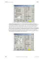
Table 1-1. System Requirements for the Thermal Transport System *
COMPONENT
FUNCTION
PPMS Resistivity Option
(Model P400)
Provides user bridge board that reads two
thermometer shoes.
PPMS AC Transport Measurement System
(Model P600)
Outputs current to heater and sample while
providing low-noise, phase-sensitive detection.
PPMS High-Vacuum Option
(Model P640)
Provides thermal isolation for measurements.
Cryopump or Turbo Pump may be used.
PPMS MultiVu Software
Version 1.1.6 or Later
Provides single user interface for PPMS and
PPMS options.
* In addition to the requirements in Table 1-1, the PPMS Continuous Low-Temperature Control
(CLTC) option (Model P800) is highly recommended. CLTC provides extended low-temperature
control.
Table 1-2. Thermal Transport System
Parameters
PARAMETER
VALUE
Pressure
High vacuum (~10-4 torr)
Temperature
1.9−390 K
Magnetic field
0−14 T when T > 20 K
If you require use of significant magnetic
fields (H > 0.1 T) at temperatures below T ~
20 K, please inquire with Quantum Design.
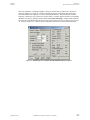
Table 1-3. Thermal Transport System Components
COMPONENT
PART NUMBER
ILLUSTRATION
Thermal Transport sample puck including
Isothermal radiation shield
4084-570
4084-575
4084-579
Figure 2-1
Two plug-in thermometer shoes
4084-580T
Figure 2-1
Plug-in heater shoe
4084-585
Figure 2-1
User’s kit
4084-569
Figure 2-3
Two nickel standard samples
4084-593
Figure 2-3
WaveROM EPROM for AC board
3084-043
Figure 2-4
Thermal Transport connection cable
3084-582
Figure 2-5
Thermal Transport software module
1-2
PPMS Thermal Transport Option User’s Manual
Quantum Design
Chapter 1
Introduction
1.2.1
Section 1.3
Measurement Modes
Purpose of Measuring Thermal Transport Properties
In measuring the thermal transport properties of a material specimen⎯such as thermal conductivity κ
and Seebeck coefficient α⎯a researcher can learn considerable information about the electronic as
well as the ionic lattice structure of that specimen. Thermal conductivity is a measure of the ability of
a material to conduct heat, so measuring this quantity provides information about scattering of heatcarrying phonons and electrons. The Seebeck coefficient describes the thermal diffusion of free charge
carriers (electrons or holes), which creates an electric field inside a material when a temperature
gradient is sustained. Much like the electrical resistivity, this property is very sensitive to subtle
changes in the electronic scattering processes and can be a powerful probe in that regard.
Taken together with electrical resistivity ρ, the thermal conductivity and Seebeck coefficient also
provide a measure of the so-called thermoelectric figure of merit Z = α2/(κρ), which is a quantity of
practical significance because it quantifies a material’s ability to transport heat by the application of an
electric current (Peltier effect), or conversely, a material’s ability to generate an electric field by
passing a thermal current (Seebeck effect, described above). The figure of merit is usually expressed
as the dimensionless quantity Z × T, where Z × T ~ 1 is a common benchmark for viability of a
material for thermoelectric applications.
1.3
Measurement Modes
The TTO system includes two measurement modes:
•
Continuous measurement mode
•
Single measurement mode
All properties measurements offered by TTO can be performed in either of these two modes.
Parameters for each measurement mode (see Section 5.3) may be specified prior to running any
measurement in that mode.
1.3.1
Continuous Measurement Mode
In continuous measurement mode, measurements are being taken continually and the adaptive software
is adjusting parameters (such as heater power and period) to optimize the measurements. This mode is
amenable to slow sweeps of system variables such as temperature or magnetic field, and it is often the
most rapid way of obtaining data because you do not have to wait for the system to reach equilibrium
before measuring. The continuous mode is also expedited by the use of a sophisticated curve-fitting
algorithm that determines the steady-state thermal properties by extrapolating from the response to a
relatively short (typically several minutes) heat pulse.
1.3.2
Single Measurement Mode
The single measurement mode is slower than continuous measurement mode because it requires that
the system reach a steady state in both the heater “off” and “on” states, which also implies that
temperature or field slewing is unavailable. The advantage of single measurement mode is that no
Quantum Design
PPMS Thermal Transport Option User’s Manual
1-3
Section 1.3
Measurement Modes
Chapter 1
Introduction
subtle curve-fitting calculations are required, so interpretation of the raw data is in principle more
straightforward. Researchers who study thermal transport properties usually employ this steady-state
technique because of its simplicity and robustness. In either style of single measurement⎯stability or
timed⎯described below in Table 1-4, data is first taken in the heater “off” state once the system
settles. After the user-specified heater power is applied, the system waits for the selected equilibrium
condi-tion before making the final measurement in the heater “on” state. You can view the live ∆T vs.
time data in the Waveform tab of the Thermal Transport control center to monitor measurement
progress.
Table 1-4. Styles for Measurements Taken in Single Measurement Mode
MEASUREMENT
STYLE
1-4
DEFINITION
Stability
System takes first measurement in heater “off” state once temperature stability
at both hot and cold sample thermometers is within a specified window, stated
either as a percentage of T or as an absolute number (in kelvin). After heat is
applied, system waits for the same stability criterion to be met before taking
final measurement. Heater power is turned off after conclusion of this measurement. User-specified timeout forces system to take a measurement at
timeout period even if stability criterion has not been met.
Timed
Sends heat pulse of user-specified duration into sample. System takes a measurement of temperatures and thermal voltages before applying heat, and then
takes final measurement at end of heat pulse.
PPMS Thermal Transport Option User’s Manual
Quantum Design
Chapter 1
Introduction
1.4
Section 1.4
Measured Thermal Properties
Measured Thermal Properties
The TTO system is set up to measure four thermal transport properties:
•
Thermal conductivity
•
Seebeck coefficient
•
Electrical resistivity
•
Thermoelectric figure of merit
If thermal conductivity, Seebeck coefficient, and electrical resistivity are all measured, then the
thermoelectric figure of merit, which is the algebraic combination of these three measurements, can be
determined.
Separate measurement protocols are provided for thermal conductivity, Seebeck coefficient, and
electrical resistivity because these individual quantities may be more accurately measured by using
excitation currents and temperature differentials optimized for each situation. Limits for the parameters defining each measurement may be specified prior to running the measurement. Section 5.3
discusses the measurement parameters.
Each measured thermal transport property may be determined in either of the two measurement modes
(continuous or single) supported by the TTO system; refer to Section 1.3. You select a measurement
mode, and then you select the thermal properties to measure in that mode.
1.4.1
Thermal Conductivity
The TTO system measures thermal conductivity κ by applying heat from the heater shoe in order to
create a user-specified temperature differential between the two thermometer shoes. The TTO system
dynamically models the thermal response of the sample to the low-frequency, square-wave heat pulse,
thus expediting data acquisition. TTO can then calculate thermal conductivity directly from the
applied heater power, resulting ∆T, and sample geometry.
1.4.2
Seebeck Coefficient
The TTO system determines the Seebeck coefficient (also called the thermopower) α by creating a
specified temperature drop between the two thermometer shoes⎯just as it does to measure thermal
conductivity. However, for Seebeck coefficient the voltage drop created between the thermometer
shoes is also monitored. The additional voltage-sense leads on these thermometer shoes are connected
to the ultra-low-noise preamplifier of the ACT system.
Quantum Design
PPMS Thermal Transport Option User’s Manual
1-5
Section 1.4
Measured Thermal Properties
1.4.3
Chapter 1
Introduction
Electrical Resistivity
The TTO system measures electrical resistivity ρ by using a precision DSP current source and phasesensitive voltage detection. The specifications for this AC resistivity measurement are essentially
identical to those for the AC Transport Measurement System (ACT) option, because the same highperformance hardware is used by both TTO and ACT. The Physical Property Measurement System:
AC Transport Option User’s Manual discusses the ACT measurements in detail.
1.4.4
Figure of Merit
The dimensionless thermoelectric figure of merit ZT is determined here simply as the algebraic
combination ZT = α2T/κρ of the three measured quantities⎯thermal conductivity, Seebeck
coefficient, and electrical resistivity⎯discussed above.
1-6
PPMS Thermal Transport Option User’s Manual
Quantum Design
Chapter 1
Introduction
1.5
Section 1.5
Theory of Operation
Theory of Operation
Benefits of the design of the TTO system include the following:
1.5.1
•
Four-terminal geometry minimizes the effects of thermal and electrical resistance of the leads
•
Continuous measurements while slewing in temperature provide high density of data
•
Careful attention to the removal of effects of temperature drift, thermal radiation, and other
systematic errors
•
Robust, easy-to-use, fully automated measurements
Hardware
When measuring in continuous mode, the DSP hardware in the Model 7100 AC Transport Controller
generates the heat pulse in the chip resistor heater on the sample, which can be described as an “on”
cycle of constant power followed by an “off” cycle of equal duration. The waveform for this pulse
was programmed specially for the TTO system in the waveROM EPROM on the AC board, so older
AC boards must have the old waveROM swapped for the new waveROM (labeled “THRMXPT
4201”) to run TTO. Section 2.2.4 discusses the waveROM EPROM in more detail.
Figure 1-2 on the following page illustrates the heat pulse as well as the temperature and voltage
response at the hot and cold thermometer shoes in an idealized sample.
1.5.2
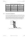
Thermal and Electrical Circuit
The thermal and electrical connections for an
idealized TTO sample are shown in Figure 1-1. For
clarity, the sample is shown mounted in the fourprobe geometry. The four basic physical elements
are illustrated: the sample, the epoxy bonds that
adhere the leads to the sample, the copper leads, and
the heater and thermometer shoe assemblies that
screw down onto the leads. For thermal conductivity
and Seebeck coefficient measurements, heat is
applied to one end of the sample by running current
through the heater (Q+/-). The temperatures Thot and
Tcold are measured at the thermometer shoes. Also
during the heat pulse, the Seebeck voltage (∆V = V+
− V−) is monitored. Heat exits the sample to the
coldfoot. Time traces of ∆T and ∆V during the heat
pulse are illustrated in Figure 1-2.
Electrical resistivity measurements are made both
before and after the heat pulse described above.
Current (I+/-) flows through the sample and the
voltage drop across the sample is monitored using
the V+/- leads.
Quantum Design
HEATER SHOE
I+
Q+
Q
COPPER LEAD
T hot
HEAT
V+
EPOXY
BOND
V
T cold
I
COLDFOOT
Figure 1-1. Thermal and Electrical
Connections for an Idealized Sample
PPMS Thermal Transport Option User’s Manual
1-7
Section 1.5
Theory of Operation
Chapter 1
Introduction
Figure 1-2. Heat Pulse and Temperature and Voltage Response at Hot and Cold
Thermometer Shoes in an Idealized Sample
Top panel:
Time trace of hot and cold thermometers during an idealized
heat pulse; note that the PPMS base temperature is slewing.
Middle panel:
Corresponding temperature ∆T and voltage ∆V differentials
across the sample, indicating thermal time constants τ1 and
τ2 and the estimate of the asymptotic differential ∆T∞.
Bottom panel: Heater power during square-wave heat pulse.
1.5.3
Software Models
In continuous measurement mode (Section 1.3.1), the software uses adaptive algorithms to optimize
measurement parameters such as heater current, heat pulse period, and resistivity excitation amplitude
and frequency. Once the ∆T vs. time data over the duration of the heat pulse is obtained, a nonlinear
least-squares fitting routine, which fits the data to the empirical formula, is launched:
∆Tmodel = ∆T∞ × {1 − [τ1 × exp(−t/τ1) − τ2 × exp(−t/τ2)]/(τ1 − τ2)}
(Equation 1-1)
where ∆T∞ represents the asymptotic temperature drop across the sample if the heater is left on
indefinitely, and τ1 and τ2 are long and short empirical time constants, respectively, for the sample (see
Figure 1-2). The fitting routine performs an exhaustive search over the space of these three parameters,
reducing the space iteratively until the parameter values that yield the minimum in the residual of the
curve fit are identified satisfactorily. Equation 1-1 is appropriate to the data taken during the heating
pulse, while the data taken during the cooling pulse is simultaneously fit essentially by changing the
sign of the model equation: ∆Tmodel,cooling = A − ∆Tmodel,heating, where A is a constant. Due to long
1-8
PPMS Thermal Transport Option User’s Manual
Quantum Design
Chapter 1
Introduction
Section 1.5
Theory of Operation
thermal diffusion times (τ1), the thermal history of the sample must be accounted for in the model, and
this is achieved by including the remanent effects of the two previous pulses in modeling the current
pulse.
The fitting routine for Seebeck coefficient data is similar, yet it is less computationally intensive. The
∆V vs. time data is read back from the DSP buffer at the end of the measurement, and after the ∆T vs.
time data is fit to obtain τ1 and τ2, a linear least-squares routine fits the data to the following equation:
∆Vmodel = ∆V∞ × {1− [τ1 × exp(−t/τ1) ± τ2' × exp(−t/τ2')]/(τ1- τ2')} + bt + c
(Equation 1-2)
where ∆V∞ is the asymptotic Seebeck voltage drop akin to ∆T∞ in equation 1-1, b and c are parameters
that describe linear drift and offset voltages, respectively, and τ2' = 0...τ1 is swept so that for each value
of τ2' a linear regression in ∆V∞, b, and c is performed. Note that “±” is used between the exponential
terms and signifies that a full search is done for each sign. The physical significance of this is that the
Seebeck coefficient of the material responsible for the short time constant τ2 (that is, the leads) may be
of the opposite sign as that for the material associated with the long time constant (that is, the sample).
This is in contrast to the case of the thermal conductivity, which is always positive. The parameter for
the linear voltage drift b is included here to account for varying thermal voltages in the wiring to the
sample and also the slow microvolt-level drift in the preamp electronics.
A similar measurement technique, previously published by Maldonado1, describes modeling of the
thermal and thermoelectric response of a sample to a low-frequency, square-wave heat pulse.
However, the thermal circuit considered in that work was considerably simpler than that which is
appropriate to TTO, and hence the modeling was done differently.
1.5.4
Estimating Errors in the Data
The software also estimates the standard deviations (σ) in the reported quantities of thermal
conductivity, Seebeck coefficient, electrical resistivity, and figure of merit ZT. This is done by
estimating the goodness of the curve fits to κ, α, and ρ by calculating the residual of the curve fit. We
make the assumption that this residual reflects the error in our estimate of the quantity (DT or DV),
and this is true when the data deviates from the curve fit in a random manner. If deviations are
systematic, as can be seen by inspecting the data in the .raw file, this indicates that the curve fit does
not properly represent the data and the quantity and that error estimates are incorrect. If this occurs,
consult Chapter 6 for troubleshooting tips. The residual for the ∆T vs. time curve fitting is calculated
as follows:
Residual = R ∆T =
2
∑ (∆Ti − ∆Ti, model )
i
(Equation 1-3)
N
where N is the number of data points making up the curve. In the measurements of κ and α, N = 64,
while for ρ, N = 128. Since the thermal conductance K = P/∆T, errors in the heater power P (see the
next section) must also be taken into account. The standard deviation in the conductivity is then
calculated:
⎛R
σ(κ) = κ × ⎜⎜ ∆T
⎝ ∆T∞
2
2
2
⎞
⎛ 0.2 × Ploss ⎞
⎛ 0.1 × T∞ × K shoes ⎞
⎛ 2IRδI ⎞
⎟⎟ + ⎜
⎟ +⎜
⎟
⎟ +⎜
P
P
⎝ P ⎠
⎝
⎠
⎝
⎠
⎠
2
(Equation 1-4)
1
Maldonado, O. Pulse method for simultaneous measurement of electric thermopower and heat conductivity at low
temperatures. Cryogenics, vol. 32, (no. 10), 1992. 908−12.
Quantum Design
PPMS Thermal Transport Option User’s Manual
1-9
Section 1.5
Theory of Operation
Chapter 1
Introduction
The first term is the residual of the curve fit mentioned above, the second term propagates the error in
the heater current I (heater resistance is R) due to the digital-analog converter, the third term is the
error in the estimation of the sample radiation term where 20% combined error in the estimation of
sample surface area and emissivity is assumed, and the last term is the error in the thermal conductance
leak from the shoe assemblies Kshoes where a 10% error in this correction is assumed (see the next
section for details on heat losses).
The error in the measurement of the thermal voltage ∆V vs. time has a similar expression as equation
1-3, so the standard deviation in the Seebeck coefficient α = ∆V/∆T is the following:
⎛R
σ(α) = α × ⎜⎜ ∆V
⎝ ∆V∞
2
2
⎞ ⎛ R ∆T ⎞
⎟⎟ + ⎜⎜
⎟⎟ .
⎠ ⎝ ∆T∞ ⎠
(Equation 1-5)
Resistivity measurements are made both preceding and following each thermal measurement so that
the average of the two ρ and σ(ρ) values is reported in the data file. The residual of the curve fits Rρ is
obtained from the stream of voltage V vs. time data as the following:
Residual = R ρ =
2
∑ (Vi − Vi, model )
i
(Equation 1-6)
N
and the standard deviation is calculated simply as
σ(ρ) = ρ ×
Rρ
(Equation 1-7)
VPP
where VPP is the peak-to-peak amplitude of the voltage vs. time signal.
The standard deviation in the figure of merit ZT is obtained by propagating the errors from each of the
measurements:
⎛ 2σ(α ) ⎞ ⎛ σ(κ) ⎞ ⎛ σ(ρ) ⎞ ⎛ σ(T) ⎞
⎟⎟ + ⎜
σ(ZT) = ZT × ⎜
⎟ + ⎜⎜
⎟
⎟ +⎜
⎝ α ⎠ ⎝ κ ⎠ ⎝ ρ ⎠ ⎝ T ⎠
2
2
2
2
(Equation 1-8)
where the last term is the standard deviation of the sample temperature over the measurement.
1-10
PPMS Thermal Transport Option User’s Manual
Quantum Design
Chapter 1
Introduction
1.5.5
Section 1.6
Start-up Checklist for Secondary Installation
Correcting for Heat Loss
Thermal conductance is determined as K = P/∆T where P is the heat flowing through the sample.
Since the heat flux cannot be measured directly, the net conducted heat through the sample is estimated
as the power (I2R) dissipated in the heater resistor, minus losses due to radiation or thermal conduction
down the leads from the shoe assemblies. Thus the conductance is determined as follows:
K [W/K] = (I2R – Prad) / ∆T − Kshoes
(Equation 1-9)
where
Kshoes = aT + bT2 + cT3
(Equation 1-10)
is a standard estimate of the thermal conductance of the shoe assemblies (a, b, and c are constants), and
Prad = σT × (S/2) × ε × (Thot4 – Tcold4)
(Equation 1-11)
is the radiation from the sample, S is the total sample surface area, ε is the infrared emissivity of the
radiating surface (see Section 5.2.2 for more information on estimating the emissivity), Thot/cold are the
average temperatures of the hot and cold thermometers during the measurement, and σT = 5.67 × 10-8
W m-2 K-4 is the Stefan-Boltzmann constant. The factor of ½ in the equation is due to the approximation that only half of the sample surface area is radiating at the hot temperature, while the other half is
at the cold temperature.
Since radiative heat losses are often very difficult to accurately estimate, you should expect errors in
measurements of thermal conductance above T ~ 300 K that are on the order of ±1 mW/K.
1.5.6
Correcting for Seebeck Coefficient of Manganin Leads
The manganin leads that connect the shoes to the connector plugs have a small Seebeck coefficient (no
more than ~ 1 µV/K at any temperature), and this has been estimated and subtracted from the “Seebeck
Coef. (uV/K)” data column in the data file. However, the column “Seebeck Volt. (uV)” is uncorrected.
1.6
Start-up Checklist for Secondary Installation
1.
Verify that the new AC board with the waveROM EPROM is installed in the Model 6000 PPMS
Controller. Refer to Sections 2.2.4 and 2.2.4.1.
2.
Verify that the Resistivity option (Model P400) is installed and the user bridge board is in the
Model 6000 PPMS Controller.
3.
Verify that all proper connections are made between the Model 6000 PPMS Controller and the
Model 7100 AC Transport Controller. Refer to Figure A-1.
4.
Verify that the High-Vacuum option (Model P640) is installed and activated.
5.
Verify that the gray Lemo cable for the Thermal Transport option is properly connected.
6.
Verify that the TTO software is installed as a PPMS MultiVu option.
Quantum Design
PPMS Thermal Transport Option User’s Manual
1-11
C
H
A
P
T
E
R
2
Hardware
2.1
Introduction
This chapter contains the following information:
2.2
•
Section 2.2 discusses and illustrates the
TTO hardware.
•
Section 2.4 discusses the High-Vacuum
option hardware that is used with TTO.
•
Section 2.3 discusses the ACT option
hardware that is used with TTO.
•
Section 2.5 explains how to calibrate new
shoe assemblies.
Thermal Transport Hardware
The TTO hardware includes the following:
•
Thermal Transport sample puck
•
Isothermal radiation shield (tube and cap)
•
Two calibrated plug-in thermometer shoes
•
One calibrated plug-in heater shoe
•
Three uncalibrated shoes: two thermometer shoes and one heater shoe
•
User’s kit
•
Two nickel calibration samples
•
Thermal Transport connection cable
The TTO system also uses ACT hardware (Section 2.3), High-Vacuum hardware (Section 2.4), and, if
required, an AC board ROM upgrade kit.
Quantum Design
PPMS Thermal Transport Option User’s Manual
2-1
Section 2.2
Thermal Transport Hardware
2.2.1
Chapter 2
Hardware
Thermal Transport Sample Puck
The Thermal Transport sample puck (Figure 2-1) plugs into the 12-pin
socket at the bottom of the PPMS sample chamber. The Thermal Transport
puck is inserted into the sample chamber by using the standard PPMS puck
extraction tool (part number 4084-110). All 12 pins on the puck are used
for thermal transport measurements (Appendix C lists pinouts). The puck
serial number is written on the plastic socket of the base.
Modularized shoe assemblies, including two temperature/voltage shoes and
one heater/current shoe, on the Thermal Transport puck connect to the
three five-pin sockets on the green printed circuit board. Each gold-plated
copper “shoe” has a hole in which the appropriate sample lead is inserted
and held in the shoe by a small stainless steel metric M1 screw. The
temperature/voltage shoe assemblies contain a Cernox 1050 thermometer
as well as a voltage lead that is soldered to the shoe itself. The
heater/current shoe assembly contains a resistive heater chip as well as an
electrical current source lead (I+) that is soldered to the shoe. At the other
end of each shoe assembly is a five-pin electrical plug on which the serial
number is written. Each shoe type⎯heater or thermometer⎯is
individually serialized. The 2-inch-long, 0.003-inch-diameter wires used
for leads on the shoe assemblies are designed to minimize thermal
conduction from the sample to the puck, and hence all are made of
manganin alloy with the exception of the current (I+) lead, which is made
of PD-135 low-resistance copper alloy. Two Sharpie permanent markers,
red and blue, have been included with the TTO system so that you can
Figure 2-1. TTO
color the alumina Cernox chip housing on each thermometer shoe, as well
Puck with Radiation
as the plastic electrical plug at the other end, to indicate the hot and cold
Shield
probes. Marking the housing is convenient because it is easy to confuse the
two sets of wires between the sockets and the shoes. The sides of the
sockets for the thermometer shoe assemblies are painted so that the middle socket is red (hot probe)
and the left-side socket is blue (cold probe). The right-hand socket, which is unpainted, is used only
by the heater shoe assembly.
The sample is connected to the puck at the coldfoot, which contains a Phillips screw and a stainless
steel clamp on the bottom that clamps onto the sample lead. This is the thermal sink for the sample, so
good thermal contact is important here. If achieving good thermal contact is a concern, a small amount
of Apiezon H Grease, which is included in the TTO user’s kit (Section 2.2.2), can be used on the
sample lead to improve contact to the coldfoot. Note that good electrical contact is also required at the
coldfoot if resistivity measurements are being made.
The copper isothermal radiation shield screws into the base of the puck and is designed to minimize
radiation between the sample and the environment. The cap is removable so that you can verify that
the leads and the sample do not touch the shield. A copper shield plate is also placed between the
sample stage and the PC board sockets to minimize radiation effects.
CAUTION!
2-2
Use care when threading the radiation shield onto the puck. The copper metal is soft, so excessive
force or misthreading of the piece can easily damage the threads.
PPMS Thermal Transport Option User’s Manual
Quantum Design
Chapter 2
Hardware
2.2.2
Section 2.2
Thermal Transport Hardware
User’s Kit
The user’s kit contains miscellaneous hardware and consumables that are needed for mounting leads
on samples as well as calibrating the spare shoe assemblies provided with the Thermal Transport
option. The convenient portable toolbox (see Figure 2-3 on the following page) helps keep the items in
the kit organized.
The contents of the user’s kit include the following.
•
Puck-mounting station
A pivoting, rotating socket is mounted to a heavy base (Figure 2-2) and holds the Thermal
Transport sample puck in a fixed position, giving you better access to the sample leads while you
are connecting the shoes or making other adjustments. Tighten the two thumbscrews on the
mounting station once the desired orientation for the puck is achieved.
Figure 2-2. Puck-Mounting Station with Puck
•
Nickel calibration samples
Two “comb-shaped” samples made of nickel are used as standards for all measured thermal
transport properties. Refer to Section 2.2.3 for more information on the nickel samples.
•
Gold-plated copper samples
Two similar comb-shaped samples of copper are provided as thermal shunts to help provide an
isothermal environment while calibrating shoe assemblies.
•
Calibration fixture
This fixture is used in conjunction with calibration software and allows the heater and
thermometer shoes to be calibrated.
•
Consumable items
These items consist of a sampler of gold-plated copper leads, including both wires and disks; a
sample of two types of epoxies for mounting leads; and a small tube of Apiezon H Grease to
increase thermal contact between the leads and shoes or the coldfoot. Chapter 4 contains more
detailed information about mounting leads to samples.
•
User tools
These tools include small slotted and Phillips screwdrivers for sample mounting, and an extractor
tool to remove the electrical connector plug ends of the shoe assemblies from the puck. This
extractor tool holds the connector plug by sliding into the grooves on each side of the plug.
Quantum Design
PPMS Thermal Transport Option User’s Manual
2-3
Figure 2-3. Thermal Transport Option User’s Kit
Chapter 2
Hardware
2.2.3
Section 2.2
Thermal Transport Hardware
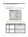
Nickel Calibration Samples
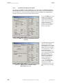
Table 2-1. Recommended Sample
Two samples of nickel metal (grade 201) are
Parameters for Nickel Calibration
supplied in the user’s kit in the form of thin plates
Samples
stamped in a four-probe “comb” configuration (see
Section 4.3) and can be used as references and
PARAMETER
VALUE
calibration verification for all standard thermal
transport measurements: thermal conductivity κ,
Cross-sectional area
0.32 mm2
Seebeck coefficient α, and electrical resistivity ρ.
Length
8.3 mm
Variations in the geometrical factor A /l on the
order of ± 5% are to be expected from sample to
Surface area
35 mm2
sample, which will be reflected in the κ and ρ data.
Emissivity
0.5
Table 2-1 lists standard dimensions for the
Ni standard. It is also recommended that the Ni
standard be mounted on the puck in the vertical configuration in order to avoid touching the radiation
shield.
2.2.4
WaveROM EPROM
The DSP board that is used with the ACMS and ACT options contains a square ROM chip that holds
waveform tables for the excitation current generated by the DSP. The TTO system requires that a new
waveform table⎯that of a square-wave pulse⎯be added to this library. All new AC boards include
this new waveROM chip, but some customers with older boards must install the new chip in order to
use the TTO system. If you are one of these customers, a new waveROM and a PLCC chip extraction
tool (AC board ROM upgrade kit) have been sent to you so that you can swap out the old chip for the
new one. Refer to Section 2.2.4.1.
Figure 2-4. WaveROM EPROM on AC Board in Model 6000 PPMS Controller
Quantum Design
PPMS Thermal Transport Option User’s Manual
2-5
Section 2.2
Thermal Transport Hardware
2.2.4.1
Chapter 2
Hardware
REPLACING THE WAVEROM CHIP
To replace the waveROM chip on the AC board, first locate the upgrade kit, which contains the PLCC
chip extraction tool and the new ROM in a small plastic box. Remove the lid of the Model 6000 so
that you can access the AC board (note that the AC board may reside in the Model 6500 Option
Controller instead). Turn off the Model 6000 and extract the old waveROM by inserting the hooks of
the extraction tool in the two slots on opposite corners of the ROM housing and gently squeezing until
the chip lifts out. To insert the new ROM, note that the upper left corner (as viewed in Figure 2-4) is
notched, and the upper side has the label attached. Press down, applying firm and even pressure to the
chip until it is seated in the housing.
2.2.5
Thermal Transport Connection Cable
The Thermal Transport connection cable (part number 3084-582) connects the sample to the Model
7100 AC Transport Controller and to the user bridge board that is in the Model 6000 PPMS Controller.
Two separate shielded cables on the connection cable plug into the Model 7100. These separate
shielded cables split the sample signal and excitation signal in order to help prevent sample signal
distortion by the excitation signal.
Labels on the cable’s connectors (Figure 2-5) identify the ports for those connectors. You should also
refer to Figure A-1, the “Thermal Transport Option Connection Diagram.”
•
The 14-pin Lemo connector plugs into the gray, color-coded port on the PPMS probe head.
•
The connector labeled “J1 (P1) User Bridge” plugs into the “P1−User Bridge” port on the Model
6000.
•
The connector labeled “J2 (P1) Sample Current Out” plugs into the “P1−Sample Current Out”
port on the Model 7100.
•
The connector labeled “J5 (P5) Sample Voltage In” plugs into the “P5−Sample Voltage In” port
on the Model 7100.
Figure 2-5. Thermal Transport Connection Cable
2-6
PPMS Thermal Transport Option User’s Manual
Quantum Design
Chapter 2
Hardware
2.2.6
Section 2.3
ACT Hardware
User Bridge Board
The TTO system employs the user bridge board to read the hot and cold Cernox thermometer shoe
assemblies that are on the sample. The user bridge board is in the Model 6000 (see Figure 2-4).
Detailed information about the user bridge board is in the Physical Property Measurement System:
Resistivity Option User’s Manual.
2.3
ACT Hardware
The TTO system uses hardware for the AC Transport Measurement System (ACT) option in order to
generate the heat pulse and read back the sample thermal voltages in the thermal measurements, and to
make the four-probe resistivity measurement on the sample.
2.3.1
Model 7100 AC Transport Controller
The driver board in the Model 7100 AC Transport Controller excites the sample by receiving and
amplifying the signal from the AC board’s digital signal processor (DSP). The preamp board in the
Model 7100 detects the sample signal and sends the signal back to the DSP so the DSP can process the
signal. The Physical Property Measurement System: AC Transport Option User’s Manual discusses
the components and operating modes of the Model 7100 in more detail.
CAUTION!
The Model 7100 provides as much as 200 mA of current when being controlled by the TTO system.
Although this is lower than the hardware limit of 2 A, this current can still damage samples in the
current path. Use only currents that can be safely handled by all hardware and samples in the circuit.
Figure 2-6. Front Panel on Model 7100 AC Transport Controller
2.3.2
AC Board
The AC board is installed in the Model 6000 PPMS Controller and is located behind the “P3−Option”
port, which is the port connecting the Model 6000 to the Model 7100. The waveROM EPROM
(Section 2.2.4) plugs into the AC board. The AC board includes a DSP, digital-to-analog converter
(DAC), current drivers, and other control electronics that are necessary to synthesize excitation signals
and process sample response signals. The DSP provides the excitation waveform and processes the
sample signal.
Quantum Design
PPMS Thermal Transport Option User’s Manual
2-7
Section 2.4
High-Vacuum Hardware
2.4
Chapter 2
Hardware
High-Vacuum Hardware
The High-Vacuum option, which operates in conjunction with the TTO system, reduces the amount of
gas in the sample chamber and thus minimizes stray thermal conduction from the heated sample. The
TTO system works with either the Turbo Pump High-Vacuum option or the Cryopump High-Vacuum
option. The details of the Turbo Pump and Cryopump high-vacuum systems are contained in the
Physical Property Measurement System: Turbo Pump High-Vacuum Option User’s Manual and
Physical Property Measurement System: Cryopump High-Vacuum Option User’s Manual,
respectively.
2.4.1
Contact Baffle
An integral part of either the Turbo Pump or the Cryopump High-Vacuum system is the contact baffle
assembly. The contact baffle makes thermal contact with the isothermal region of the sample chamber,
which is just above the puck. The thermal contact between the contact baffle and the isothermal region
helps create a more uniform thermal environment for the puck by causing the contact baffle to be at the
same temperature as the chamber walls that are near the puck. This is important when high vacuum is
enabled; high vacuum reduces the amount of thermal exchange gas in the sample chamber.
You insert the contact baffle into the brass fitting that is at the bottom of the baffle assembly (see
Figure 2-8B). To help safeguard the contact baffle, use it only when you are using the High-Vacuum
option. Handle the contact baffle with care, and avoid touching the delicate outer contact fingers. The
charcoal holder is used to achieve the best vacuum at low temperatures and should always be screwed
onto the bottom of the contact baffle when in the high-vacuum state. However, when performing a
temperature calibration of any sample hardware, such as TTO shoe assemblies, the charcoal holder
should be removed to ensure that adequate thermal exchange gas remains in the sample chamber at low
temperature.
Figure 2-7. Baffle Assembly with Contact Baffle
A. Charcoal Holder Removed for Puck Calibration
B. Charcoal Holder Installed for Normal Operation
Figure 2-8. Close-up View of Contact Fingers and Charcoal Holder on Contact Baffle Assembly
2-8
PPMS Thermal Transport Option User’s Manual
Quantum Design
Chapter 2
Hardware
2.5
Section 2.5
Calibrating New Shoe Assemblies
Calibrating New Shoe Assemblies
A spare set of uncalibrated shoe assemblies (two thermometers and one heater) is included in the TTO
user’s kit. You can easily calibrate the shoe assemblies by using the calibration wizard (see Figure 210) that is accessed in the Advanced tab of the Thermal Transport control center. To calibrate new
shoe assemblies, the calibration fixture (3084-576) must first be plugged into the Thermal Transport
puck as shown in Figure 2-9.
The vertical plate that is usually mounted between the sample and the plugs for the shoe assemblies
must be removed before plugging in the calibration fixture. Unscrew the two Phillips-head screws at
the base of the plate only enough to remove the plate, and then retighten the screws to hold the PC
board. Use caution so that you do not strain the wiring on the bottom side of the PC board: do not lift
or turn the board or pinch any wires when retightening the screws.
NOTE
If a heater shoe is being calibrated, plug it into the left-hand socket (the socket closest to the marking
“PCB 3084-576” –see Figure 2-9). If calibrating thermometer shoe assemblies, plug them into the
other two sockets, with “Thermometer A” in the middle socket and “Thermometer B” in the right-hand
socket. Note that wiring in the shoe assemblies is symmetric, so plugging in the connectors in either of
the two possible orientations will make the proper electrical connections.
Next, locate a gold-plated copper calibration sample from the TTO User’s Kit. Bend the leads on the
sample so that you can mount it as shown in Figure 2-9. Then mount the copper sample to the cold
foot and mount the copper shoes to the sample. When mounting the heater shoe, make sure the copper
sample does not touch the solder pad of the heater resister, which could cause an electrical short.
Note the serial numbers of each shoe assembly. Then screw the shield onto the TTO puck. Unscrew
the shield cap and make sure none of the copper shoes are touching any part of the puck or the shield.
Replace the shield cap; then insert the puck into the PPMS. Remove the charcoal carrier on the contact
baffle assembly (see Section 2.4.1) to ensure exchange gas is not cryopumped at low temperatures.
Place the baffle set inside the sample chamber. Then purge and seal the sample chamber.
In the calibration wizard window, check the box for the thermometers and/or heaters you wish to
calibrate and enter their serial numbers. The default temperature range should be 1.8 to 400 K. The
heater parameters have been selected to optimize the signal for the 2kΩ heater resistors supplied.
Press the “Start” button to begin calibration, which will last approximately 16 hours.
After calibration is complete, you must make the appropriate changes to TTO initialization file
TTO.INI if you wish to use the newly calibrated shoe assemblies immediately. See Section 3.2.
Quantum Design
PPMS Thermal Transport Option User’s Manual
2-9
Section 2.5
Calibrating New Shoe Assemblies
Chapter 2
Hardware
THERM B
THERM A
HEATER
Figure 2-9. Calibration Fixture Plugged into TTO Puck and Illustrating Sockets for
Each Shoe Assembly
Figure 2-10. Thermal Transport Calibrate Thermometers and Heater Wizard
2-10
PPMS Thermal Transport Option User’s Manual
Quantum Design
C
H
A
P
T
E
R
3
Software
3.1
Introduction
This chapter contains the following information:
3.2
•
Section 3.2 presents an overview
of the TTO system software.
•
Section 3.4 discusses the TTO data
files.
•
Section 3.3 discusses the Thermal
Transport control center.
•
Section 3.5 explains how to examine
data saved to a TTO data file.
Overview of Thermal Transport Software
The TTO software module is integrated into the Quantum Design PPMS MultiVu environment.
Version 1.1.6 or greater of the PPMS MultiVu software is required to install the TTO software. For
software installation instructions, see Appendix A.
TTO is designed to be used by both experts and newcomers to the study of thermal transport
properties. To accommodate this spectrum of users, the software interface is multi-leveled so that
beginners can easily set up and perform measurements at the top level while experts can choose to
navigate into submenus in order to adjust various parameters or customize measurements.
TTO measurements can be run either interactively at the dialog or in a sequence program. While the
TTO software is active in PPMS MultiVu, the command TTO Measure appears in the sequence
command bar under the Measurement Commands heading. This command is used to start, stop, or
change measurement parameters within a sequence file. Users who are familiar with measurement
sequence commands for other Quantum Design options will find an important difference in the use of
the TTO Measure command compared to other options, where sequence execution is typically paused
until a measurement command is completed. This principle is not appropriate for continuous TTO
measurements because these can be performed while a system parameter such as the temperature is
swept slowly. Therefore, the TTO Continuous Measure command initiates measurements and the
sequence execution immediately continues. TTO measurements are taken until the TTO Stop
sequence command is issued. The TTO single measurement sequence commands are more similar to
the traditional measurement commands. During these measurements, sequence execution is paused
until the measurement is completed because single measurements operate on the condition that system
parameters are stable during the measurement.
Quantum Design
PPMS Thermal Transport Option User’s Manual
3-1
Section 3.2
Overview of Thermal Transport Software
Chapter 3
Software
The data file for TTO measurements (sample.dat, where sample is the file name you select)
contains the results for each measurement that was completed successfully. The raw data from all
measurements can also be saved in a separate file (sample.raw).
As soon as the TTO software is activated in PPMS MultiVu, the Thermal Transport Log window
(Figure 3-1) opens and indicates which thermometer and heater calibration files will be used. These
settings, as well as several other parameters, can be edited in the Tto.ini initialization file located in
the QdPpms\ThermalTransport\System directory. The thermometer and heater calibration
files are located in the QdPpms\ThermalTransport\Calibration directory. The TTO log
can be viewed by using the View¾TTO Status Log menu command.
Figure 3-1. Thermal Transport Log Window
3.2.1
Measurement Units
Thermal conductivity κ is typically stated in either units of watt/(meter-kelvin), written W/m-K, or in
mW/cm-K. In the TTO software, the units of W/m-K are used for thermal conductivity. The Seebeck
coefficient is expressed most conveniently in µV/K, because in many electrical conductors α ~ µV/K
at room temperature. The electrical resistivity ρ is stated in units of ohm-meter (Ω-m). The thermoelectric figure of merit ZT = α2T/ρκ is dimensionless when MKS units are chosen for each quantity;
that is, α[V/K], T[K], ρ[Ω-m], and κ[W/m-K].
3-2
PPMS Thermal Transport Option User’s Manual
Quantum Design
Chapter 3
Software
3.3
Section 3.3
Thermal Transport Control Center
Thermal Transport Control Center
The TTO software module has a control center that includes all frequently selected Thermal Transport
commands. With its easy-to-use tab format and software prompts, the control center makes basic
system operations, such as installing samples, creating data files, and setting up and running
immediate-mode measurements, more natural and convenient. The Thermal Transport control center
opens as soon as the Thermal Transport option is activated in PPMS MultiVu, and although it may be
minimized, does not close until the option is deactivated. Figures 3-2 through 3-6 illustrate the tabs in
the Thermal Transport control center.
3.3.1
Control Center Tabs
The Install tab automatically
opens when the software starts,
and it assists you in sample
installation or removal by
providing sample chamber
Vent and HiVac buttons and
by also providing an install
wizard with more extensive,
step-by-step instructions for
setting up a measurement.
Figure 3-2. Control Center Install Tab
The Data File tab lets you
open a new TTO data file or
append to an existing TTO
data file. You can also use the
tab to view data and select
whether raw thermal transport
data is saved in a .raw file.
See Section 3.4 for information
on TTO data file formats.
Figure 3-3. Control Center Data File Tab
Quantum Design
PPMS Thermal Transport Option User’s Manual
3-3
Section 3.3
Thermal Transport Control Center
Chapter 3
Software
The Sample tab displays the
sample name, comments,
geometry and radiation
estimates for the currently
open data file. These parameters can be changed only by
opening a new file in the Data
File tab. Chapter 4 has more
information on how to mount
sample leads and estimate
properties such as the sample’s
infrared emissivity.
Figure 3-4. Control Center Sample Tab
The time traces of the most
recent raw data, along with the
fitted curves, are displayed in
the Waveform tab. As a
visual aid, the heater pulse is
shown schematically in the
Waveform tab as a yellow
square wave in both the
thermal conductivity and
Seebeck graphs.
Figure 3-5. Control Center Waveform Tab
Clicking the right mouse button inside the graph window in the Waveform tab opens a menu that
allows selection of thermal conductivity, Seebeck coefficient, or resistivity results, and whether to
plot the fitted curve along with raw data. The title of the graph indicates which data is being
displayed. For thermal conductivity data, “Temperature Delta” refers to the difference between hot
and cold thermometers, while for Seebeck measurements “Seebeck Voltage” refers to the voltage
difference between the hot and cold shoes.
To the right of the graph are listed three parameters that briefly summarize the curve fitting results:
the total amplitude obtained by the curve-fitting routine (equivalent to Delta Temp. or Seebeck
Volt. in the data file), the long time constant in the measurement (that is, τ1 ⎯this is not relevant to
resistivity data), and the residual of the curve fit (that is, the error estimate for the reported total
amplitude). Section 1.5 contains more information on the AC measurements and error estimation in
TTO data.
In the Waveform tab, you can also zoom to examine details of the data by dragging the mouse from
the upper left to the lower right corner of the graph while holding down the left mouse button. To
zoom out, drag the mouse in the opposite direction while holding down the button, or select Zoom All
in the pull-down menu, which is accessed by clicking the right mouse button in the graph.
3-4
PPMS Thermal Transport Option User’s Manual
Quantum Design
Chapter 3
Software
Section 3.3
Thermal Transport Control Center
The Advanced tab includes a
software wizard that allows
you to calibrate new TTO shoe
assemblies (heater and/or
thermometers) in the PPMS.
The calibration fixture (3084576) from the user’s kit is used
in conjunction with this
software wizard. The
Restart... button is used if you
previously cancelled a
calibration and want to restart.
Refer to Section 2.5 for more
information on calibrating shoe
assemblies.
Figure 3-6. Control Center Advanced Tab
Other features on the Advanced tab include a heater test in which you select the desired heater current
to apply, as well as an option to swap the software’s assignment of hot and cold thermometers.
3.3.2
Measurement Menu
Selecting the Measure... button at the bottom of the Thermal Transport control center opens the
Thermal Transport Measurement dialog box, which allows you to run immediate-mode TTO
measurements without having to write a sequence file. Three tabs⎯Settings, Thermal, and
Resistivity, shown in Figures 3-7, 3-8, and 3-9⎯are immediately visible in the Thermal Transport
Measurement dialog.
In the Settings tab (Figure 3-7) you determine basic settings for all measurements. First you select
which of the four thermal transport quantities are to be measured. Note that checking Figure of Merit
(ZT) automatically selects all measurements because they are all required to assess ZT. You have the
option to save “marginal” results, which would otherwise be discarded, to the data file. Marginal
measurements are defined as those for which the software was able to determine a quantity, but the
regression errors of the curve fits were between 50% and 200% (the measurement is considered failed
if the regression is higher than 200%). The Discard First N Results check box is included because
the first several measurements often have large errors due to the measurement parameters not being
optimized. Choosing N = 3 is typically adequate, if you choose to discard any results. In the Next
Measurement box you can specify the period and heater power for the next thermal measurement
cycle, even after measurements have started. Note that any changes made in this box are saved only if
the Set button is selected. Selecting Clear restores the values that were last input.
Quantum Design
PPMS Thermal Transport Option User’s Manual
3-5
Section 3.3
Thermal Transport Control Center
Chapter 3
Software
Figure 3-7. Settings Tab in Thermal Transport Measurement Dialog Box
Settings and limits for thermal measurements (thermal conductivity and Seebeck coefficient) are
determined in the Thermal tab (Figure 3-8). These settings and limits include limits of heater period
and power and expected limits of Seebeck readback voltage, as well as target amplitude for the heat
pulse (expressed as percentage of sample temperature) and target value of period ratio, which is
defined as measurement period divided by the time constant (tαυ1) of the sample (see Section 3.4.3 for
more information on these quantities). Any changes made in this tab are saved only if the Set button in
the tab is selected. A ToolTip displays hardware limits for the heater power if the cursor is placed over
the panels showing the heater power limits. Note that a period ratio of at least 8 is recommended
because choosing a value lower than this has been shown to produce artifacts in the thermal transport
measurements due to insufficient data for the software model.
Figure 3-8. Thermal Tab in Thermal Transport Measurement Dialog Box
3-6
PPMS Thermal Transport Option User’s Manual
Quantum Design
Chapter 3
Software
Section 3.3
Thermal Transport Control Center
Due to the complexity of making an adaptive resistivity measurement, a separate tab is devoted to
resistivity (Figure 3-9) so that you can have maximum freedom in setting limits such as min/max
excitation and min/max frequency, as well as measurement duration. The measurement excitation
frequency is allowed to vary so that a 90% resistive (that is, in-phase) signal is obtained. Autoranging
parameters may also be changed, with the default being Sticky Autorange. Changes made in this tab
are saved only if the Set button in the tab is selected. See the Physical Property Measurement System:
AC Transport Option User’s Manual for more information on resistivity measurement parameters.
Figure 3-9. Resistivity Tab in Thermal Transport Measurement Dialog Box
Quantum Design
PPMS Thermal Transport Option User’s Manual
3-7
Section 3.3
Thermal Transport Control Center
3.3.2.1
Chapter 3
Software
OPTIONS FOR ADVANCED USERS
Two more tabs, the Mode tab and the Advanced tab, are made visible in the Thermal Transport
Measurement dialog box by clicking on the right-pointing arrow that is next to the tab names at the
top of the dialog box. Clicking on the left-pointing arrow hides the Mode and the Advanced tabs.
Generally, these two tabs are of interest only to advanced users.
You use the Mode tab to select
whether to take continuous
measurements (default) or
single, steady-state measurements. There are two modes
of single measurement:
stability or timed. Section 1.3
describes the measurement
modes in more detail.
Figure 3-10. Mode Tab in Thermal Transport Measurement
Dialog Box
Figure 3-11. Advanced Tab in Thermal Transport
Measurement Dialog Box
3-8
PPMS Thermal Transport Option User’s Manual
The PPMS data logging dialog
can be accessed from the
Advanced tab in the event that
you would like to select which
PPMS status items are written
to the TTO data file. Table 3-1
on the following page
describes the parameters that
can be monitored on the PPMS
data logging dialog. The
Reprocess command allows
you to recompute thermal
transport results from an
existing TTO data file
(*.dat) by changing the
sample’s estimated geometry
and emissivity, and the
command allows you to write
these results out to a new data
file.
Quantum Design
Chapter 3
Software
Section 3.3
Thermal Transport Control Center
Table 3-1. PPMS system data items that can be saved to the TTO measurement data file.
Items in bold and all capital letters are always written to the data file.
ITEM
DEFINTION
GENERAL STATUS
General system status, coded. Appendix B explains how to
interpret status code.
TEMPERATURE
System temperature, measured at base of sample chamber.
MAGNETIC FIELD
Magnetic field.
Sample Position
For use with rotator probes*.
SAMPLE PRESSURE
Pressure in sample chamber, measured in torr.
Digital Inputs
Eight-bit status of selected inputs.
Dr Ch 1−2 Current
Current delivered by selected driver output channel.
Dr Ch 1−2 Power
Power delivered by selected driver output channel.
Brg Ch 1−4 Resistance
Resistance of selected user bridge channel.
Brg Ch 1−4 Excitation
Excitation current of selected user bridge channel.
Sig Ch 1−2 Input Voltage
Input voltage for selected signal channel.
Map 20−29
User-designated data items. Reserved for hot and cold
sample thermometers.
MAP 21−22
* Rotator probes are not currently available for use with TTO.
3.3.3
System Status
Features in the Thermal Transport control center provide constant updates of TTO status.
•
The Status bar at the bottom of the Thermal Transport control center succinctly describes the
progress of an on-going measurement and summarizes the results of the last measurement.
Color-coded warning and error messages in the Status bar alert you to possible problems.
Warning messages appear on a yellow background. Error messages appear on a red background.
•
The Waveform tab in the Thermal Transport control center (Figure 3-5) displays raw data
waveforms and curve fits for any of the measurements, and the tab indicates the fitting
parameters of signal amplitude, time constant τ1 (where relevant) and the residual for the fit.
•
The measurement Progress bar and countdown timer in the bottom right corner of the Thermal
Transport Measurement dialog box indicate the time remaining before the measurement is
complete. Refer to Figure 3-7. In the Progress bar, yellow indicates the heater “on” state while
blue indicates “off.”
•
The right side of the Thermal Transport Measurement dialog box summarizes the most recent
measurement and the parameters (period and power) used for the current measurement. Refer to
Figure 3-8. Note that if the cursor is placed over the displayed results, a ToolTip shows the
estimated error for the results.
•
The Thermal Transport Log window (Figure 3-1) keeps a record of all messages that appear in
the Thermal Transport control center Status bar. The TTO status log is saved in the file
TtoLog.txt, which is in the directory C:\QdPpms\ThermalTransport\LogFiles.
Quantum Design
PPMS Thermal Transport Option User’s Manual
3-9
Section 3.4
Thermal Transport Data Files
3.4
Chapter 3
Software
Thermal Transport Data Files
Thermal Transport measurement data is stored in measurement data files and raw measurement data
files. Measurement data files, which have a .dat extension, store relevant sample measurement data
and selected system data for any number of measurements taken by any of the Thermal Transport
measurement types. Raw measurement data files, which have a .raw extension, store raw temperature versus time (thermal conductivity) and voltage versus time (Seebeck and resistivity) data as well
as the software’s fits to the data. Raw data is saved only if the Capture Raw Data check box in the
Data File tab (Figure 3-3) is selected. The system data items that may be recorded are user
configurable (Section 3.4.2).
The results from measurements, whether made in continuous or single mode, are automatically saved if
a data file is open. Measurement and system data is appended to the selected data files and is never
overwritten. The Data File tab in the Thermal Transport control center identifies the selected measurement data file and raw measurement data file and includes a Browse command button that enables
data file selection and creation. The name of the selected measurement data file is also displayed in
the title bar of the Thermal Transport control center.
3.4.1
Saving Raw Thermal Transport Data
Raw thermal transport data is saved to a separate raw measurement data file that has the identical base
name as the measurement data file, but a .raw file extension instead of a .dat extension. Saving the
raw data can be useful when you are deciding which measurement parameters to use or if you are
concerned about signal quality. A clean, single-wavelength sine wave is optimal in the case of AC
resistivity measurements. In the cases of thermal conductivity and Seebeck measurements, the fitted
model curve can be plotted along with the raw data so that you can easily assess the quality of the
results. However, saving raw data creates very large data files.
Raw thermal transport data is saved only if a measurement data file is selected and the software is
prompted to capture raw data. Enabling the Capture Raw Data check box in the Thermal Transport
control center’s Data File tab (Figure 3-3) prompts the software to save raw data. By default, this
check box is not selected.
3.4.2
Data File Header
The data file header contains file and sample property information that is defined when the data file is
created. Information written to the data file header cannot be subsequently changed in PPMS MultiVu.
The file information that can be written to the header consists of the title assigned to the graph view of
the data file. The sample property information consists of the sample dimensions and emissivity. User
comments can also be written to the header. All this information appears in the INFO declara-tions of
the header. The Physical Property Measurement System: PPMS MultiVu Application User’s Manual
contains more information on data file headers.
When you create a data file, the software prompts you to enter the physical dimensions and an estimate
of the emissivity for the sample whose measurement data will be saved to the file. To enable you to do
this, the data entry fields in the Thermal Transport control center’s Sample tab are enabled. As soon
as you define the sample properties and select OK, all data entry fields in the Sample tab (Figure 3-4)
are disabled again.
3-10
PPMS Thermal Transport Option User’s Manual
Quantum Design
Chapter 3
Software
Section 3.4
Thermal Transport Data Files
Because the data file header identifies a particular sample, changing samples without changing data
files can destroy the validity of the data in the file. Therefore, you are encouraged to use the
automated routines in the Thermal Transport control center. These automated routines prompt you
for new data file(s) and new sample information after you install a different sample.
NOTE
3.4.3
Format of Measurement Data Files
Table 3-2 lists and describes all data columns in the Thermal Transport data file. Section 5.3 provides
more information on some of these fields.
Table 3-2. Fields in Thermal Transport Measurement Data File
ITEM
DEFINITION
Time Stamp
Time of measurement data point, expressed in minutes or
seconds, and as an absolute time or relative to the start time
of the data file.
Status (code)
PPMS system status. Identical to General Status in Table 31.
Error (code)
TTO error code. Appendix B describes how to interpret the
code.
Magnetic Field (Oe)
Magnetic field.
Sample Temp. (K)
Average sample temperature during measurement.
Conductivity (W/K-m)
Sample thermal conductivity.
Cond. Std. Dev.
Error (standard deviation) in thermal conductivity
measurement.
Seebeck Coef. (uV/K)
Sample Seebeck coefficient in units of µV/K.
Seebeck Std. Dev.
Error in Seebeck coefficient measurement.
Resistivity (Ohm-m)
Sample resistivity.
Resist. Std. Dev.
Error in resistivity measurement.
Figure of Merit [ZT]
Dimensionless thermoelectric figure of merit ZT.
Merit Std. Dev.
Error in ZT measurement.
Delta Temp. (K)
Extrapolated (asymptotic) temperature drop ∆T across heated
sample.
Conductance (W/K)
Net thermal conductance of sample. See Section 1.5.5.
Raw Conductance (W/K)
Raw thermal conductance, that is, (Heater Power)/(Delta
Temp.).
Seebeck Volt. (uV)
Extrapolated (asymptotic) Seebeck ∆V across heated sample.
Resistance (Ohm)
Sample resistance.
(continues)
Quantum Design
PPMS Thermal Transport Option User’s Manual
3-11
Section 3.4
Thermal Transport Data Files
Chapter 3
Software
Table 3-2. Fields in Thermal Transport Measurement Data File (Continued)
ITEM
DEFINITION
Min. Temp. (K)
Minimum temperature at either hot or cold thermometer
during measurement.
Max. Temp. (K)
Maximum temperature at either hot or cold thermometer
during measurement.
Temp. Rise (K)
Rise in temperature of the hot thermometer due to the applied
heat pulse. Should be close to user-requested value set in
Thermal tab.
Req. Htr. Power (W)
Requested heater power, in watts.
Heater Power (W)
Actual heater power.
Rad. Loss (W)
Estimated power loss due only to radiation from sample. See
Section 1.5.5.
Cond. Pwr. (W)
Estimated net power conducted through sample.
Heater Current (mA)
Current through heater.
Res. Drive (mA)
Current drive used for resistivity measurement.
Res. Freq. (Hz)
Frequency used for resistivity measurement.
Period (sec.)
Period for heater on/off square-wave pulse.
Period Ratio
Ratio of period/tau1.
tau1 (sec.)
Long thermal time constant of sample and shoes.
tau2 (sec.)
Short thermal time constant of sample and shoes.
Seebeck Gain
Total gain (preamp and DSP) for Seebeck data point.
Resist. Gain
Total gain (preamp and DSP) for resistivity.
System Temp. (K)
PPMS block system temperature.
Sample Position (deg.)
Used with rotator probes; not used in TTO*.
Brg Ch 1−4 Resistance
Resistance of selected user bridge channel.
Brg Ch 1−4 Excitation
Excitation current of selected user bridge channel.
Sig Ch 1−2 Input Voltage
Input voltage for selected signal channel.
Digital Inputs (code)
Eight-bit status of selected inputs.
Dr Ch 1−2 Current
Current delivered by selected driver output channel.
Dr Ch 1−2 Power
Power delivered by selected driver output channel.
Pressure
Sample chamber pressure, in torr.
Map 20−29
Map 21−22
User-designated data items. Reserved for hot and cold sample
thermometers.
* Rotator probes are not currently available for use with TTO.
3-12
PPMS Thermal Transport Option User’s Manual
Quantum Design
Chapter 3
Software
3.4.4
Section 3.4
Thermal Transport Data Files
Format of Raw Data Files
If the Capture Raw Data check box is selected in the Data File tab in the Thermal Transport control
center (Figure 3-3), raw measurement data is recorded to a data file. For thermal conductivity and
Seebeck coefficient measurements, raw data also includes results from the thermal model. For
resistivity measurements, raw data includes the excitation current and signal voltage.
Table 3-3. Fields in Thermal Transport Raw File
ITEM
Quantum Design
DEFINITION
Comment
System status and TTO software comments.
Time Stamp
Time of measurement data point, expressed in
minutes or seconds, and as an absolute time or
relative to the start time of the data file.
T-Hot (K)
Temperature of sample hot thermometer.
T-Cold (K)
Temperature of sample cold thermometer.
T-Sys (K)
Temperature of PPMS system thermometer.
Delta T (K)
Temperature drop across sample thermometers.
Model Delta T (K)
Curve fit of ∆T to software thermal model.
Seebeck (uV)
Raw Seebeck voltage.
Model Seebeck (uV)
Curve fit of Seebeck to software thermal model.
Res. Excit. (mA)
Excitation current from resistivity measurement.
Res. Signal (mV)
Signal voltage from resistivity measurement.
PPMS Thermal Transport Option User’s Manual
3-13
Section 3.5
Data Examination
3.5
Chapter 3
Software
Data Examination
To examine the current TTO .dat data file in PPMS MultiVu, you can select the View button in the
Data File tab in the control center. If raw data is also being saved, the raw file can be opened by using
the File¾Open menu command. The Physical Property Measurement System: PPMS MultiVu
Application User’s Manual discusses the graphing and data-viewing formats in detail.
The ExportData.exe program, located in the QDPPMS\Tools directory, can be used to export
specific columns and portions of the data file header from any data file.
Errors encountered by the PPMS during TTO data acquisition are listed in the TTO status log (see
Section 3.3.3). In addition, an Error Count dialog is opened if any individual TTO measurement
fails. A running total of the error counts is displayed and brief one-line descriptions of the last three
errors are listed in the window. If this dialog is closed, it can be accessed by using the View¾TTO
Error Count menu command. Selecting the Reset button will zero the displayed error totals for each
measurement, but will not affect the TTO log file.
Figure 3-12. Error Count Dialog Box
3-14
PPMS Thermal Transport Option User’s Manual
Quantum Design
C
H
A
P
T
E
R
4
Sample Preparation
4.1
Introduction
This chapter contains the following information:
4.2
•
Section 4.2 discusses sample-mounting
considerations.
•
Section 4.3 explains how to check
the sample contact.
•
Section 4.3 discusses the two-probe and
four-probe lead configurations.
•
Section 4.5 explains how to use the
puck-mounting station.
Sample-Mounting Considerations
Four leads must be attached to the sample in order for the TTO system to take thermal (and electrical)
measurements. These four leads are a heater (and current I+), a heat sink (and current I−), and two
temperature (and voltage) probes that are along the length of the sample. The TTO system takes both
thermal and electrical measurements by using the same probes, so measurements of thermal
conductivity, thermopower, and electrical resistivity can be performed in one pass without remounting
the sample.
It is important that the resistance⎯either thermal or electrical⎯at the interface between the leads and
the sample be minimized. This is especially important when a two-probe measurement (Section 4.3.1)
is performed, because any contact resistance is directly reflected in the measured sample thermal and
electrical resistance. In addition, you are advised to minimize the thermal diffusion time in the leads
by keeping them short (2−3 millimeters, if possible), because this expedites the measurement process.
Quantum Design
PPMS Thermal Transport Option User’s Manual
4-1
Section 4.2
Sample-Mounting Considerations
4.2.1
Chapter 4
Sample Preparation
Geometry
The geometry of the sample is constrained due to a variety of considerations, the most obvious of
which is the Thermal Transport sample puck. Mounted vertically on the puck, a sample cannot be
much longer than 20 mm, while the minimum convenient sample length is typically 3 mm.
Another aspect to consider is the thermal diffusion time in the sample, defined as τ ~ C/K, where
C(Joule/K) is the heat capacity and K(Watt/m) is the thermal conductance of the sample. This places
an operational lower limit on K so that the measurement time does not become excessively long (one
measurement is typically designed to be ~ 8 × τ; see Section 1.5). Since K = κ × A/l, where κ(W/m K) is the thermal conductivity, A is the cross-sectional area of the sample, and l is the length, this
implies a lower limit on A/l for a given value of κ. Another relation that can be easily derived from the
above equations is τ ~ cp × l2/κ, where cp(J/m3 - K) is the specific heat of the material. This implies
that, for a given material, the time constant simply scales quadratically with the length, with a typical
practical upper bound of lmax ~ 10 mm on samples.
While the thermal diffusion time τ places a lower limit on A/l, the heater power P(W) = κ × ∆T × (A/l),
where ∆T ~ 0.03 × T (typical value) is the temperature drop across the sample, sets the upper limit on
A/l because the heater is limited by the 10-V compliance limit of the Model 7100 current source. For
an R = 2 - kΩ chip heater, Pmax = V2/R = 50 mW.
Keep in mind that the constraints mentioned here are most stringent at high T, where τ is generally
longer and the required ∆T is larger. Table 4-1 gives some examples of sample geometries and the
range of measurable thermal conductivities based on the above considerations and using a 2-kΩ heater.
Table 4-1. Sample Geometries and Range of Measurable Thermal Conductivities
DIMENSIONS
4-2
× (A) (mm3)
HIGH T CONSTRAINTS
ON κ (W/m - K)
SAMPLE
L
Brick
8 × (2 × 2)
2−30
Needle
10 × (1 × 1)
10−150
Pill
3 × (5 × 5)
0.1−1.5
PPMS Thermal Transport Option User’s Manual
Quantum Design
Chapter 4
Sample Preparation
4.2.2
Section 4.2
Sample-Mounting Considerations
Lead-Mounting Epoxies
After deciding on an appropriate geometry for the particular thermal transport measurement you will
take (see Section 4.2.1), you cut and sand the sample so that its surfaces are clean.
The epoxies used to attach leads to samples should be chosen for the following:
•
Strength in bonding to the particular sample material
•
High thermal conductivity
•
Convenience of the curing schedule
In addition, any time the thermoelectric or electrical properties will be measured, an electrically
conducting silver-filled epoxy must be used. On the other hand, the primary advantage of electrically
nonconductive epoxies is their very high strength.
Use a generous (but not excessive) amount of epoxy when attaching leads so that the bond is strong
and provides very good thermal contact.
NOTE
The sample-mounting kit contains starter samples of epoxies, including Silver-Filled H20E from
Epoxy Technology, Inc., and nonconductive Tra-Bond 816H01 from Tra-Con, Inc. Product
specifications and Materials Safety Data Sheets (MSDS’s) for both epoxies are included in the epoxy
kit.
4.2.2.1
SILVER-FILLED H20E EPOXY
Small amounts of parts A and B (labeled on the containers) should be thoroughly mixed in an
approximately 1:1 ratio on a clean, dry, and nonabsorbing surface, using care that no crosscontamination of the remaining portions in the jars occurs. After applying the mixture to the leads and
sample and attaching the leads, you can bake the sample at ~ 150°C for about 5 minutes. See the
vendor’s product data sheet included in the epoxy kit for more information, including other possible
curing schedules.
4.2.2.2
TRA-BOND 816H01 EPOXY
This electrically nonconductive epoxy is provided in one-use, 2-gram packets. Because 2 g is a much
larger amount of epoxy than is needed for one sample, Quantum Design recommends preparing several
samples at the same time. To mix, slide off the plastic clamp and knead both chambers thoroughly so
that the texture feels uniform; this occurs after approximately 2 minutes of mixing. Cut open one end
of the packet to dispense epoxy, and allow 24 hours for epoxy bonds to cure. Note that the liquid
epoxy may have a grainy appearance; this is normal.
Quantum Design
PPMS Thermal Transport Option User’s Manual
4-3
Section 4.3
Two-Probe and Four-Probe Lead Configurations
4.3
Chapter 4
Sample Preparation
Two-Probe and Four-Probe Lead Configurations
There are two methods of mounting the electrical/thermal leads on a sample. These two different
methods present a trade-off between convenience of mounting and accuracy of measurement.
4.3.1
Two-Probe Lead Configuration
The two-probe lead configuration method is the most convenient because it involves attaching only
two leads, but this method sacrifices accuracy because heater/I+ and Thot /V+ share one lead while
coldfoot/I− and Tcold /V− share the other lead (Figure 4-1). Thus, the thermal and electrical contact
resistances between the leads and sample contribute to the measured quantities. You should use the
two-probe lead configuration method only when the thermal and electrical resistances of the sample
are far greater than those of the leads. Examples of samples mounted in this fashion are shown in
Figure 4-1, where both bar-shaped and disk-shaped copper leads are used.
A.
Two-Probe Lead Configuration Using
Disk-Shaped Copper Leads
B.
Two-Probe Lead Configuration
Using Bar-Shaped Copper Leads
Figure 4-1. Examples of Leads Mounted in Two-Probe Configuration
Note that the thermal conductance of the epoxies decreases very rapidly below 100 K, so the thermal
contact resistance may be significant at low temperature even if it is not at room temperature. If you
know the cross-sectional area and the approximate thickness of the epoxy used, then you can estimate
the contact resistance due to the thermal resistance of the epoxy using the data in Table 4-2 and the
equation for the thermal resistance:
1/K = 1/κ × l/A,
where A is the cross-sectional area of the bond and l is the thickness of the epoxy in the bond.
4-4
PPMS Thermal Transport Option User’s Manual
Quantum Design
Chapter 4
Sample Preparation
Section 4.3
Two-Probe and Four-Probe Lead Configurations
Table 4-2. Approximate thermal conductance of epoxies
TEMPERATURE
(K)
4.3.2
SILVER-FILLED H20E EPOXY
κ (W/m - K)
TRA-BOND 816 H01 EPOXY
κ (W/m - K)
300
2
1
100
1
0.5
30
0.5
0.2
10
0.2
0.09
5
0.1
0.03
2
0.03
0.01
Four-Probe Lead Configuration
Use a four-probe lead configuration method when sample resistivity (thermal or electrical) is too low
to allow you to neglect the contribution of lead contact resistance. Thus, the four probes are attached
individually and you avoid the problem of contact resistance at the Thot /V+ and Tcold /V− probes. This
is because very little thermal or electrical current passes into the copper shoes from the sample and
hence they approximate much better the ideal of passive probes of the sample’s temperature and
voltage profile. Note that care must be taken to keep separate the epoxy pads on the sample, or else
this advantage is compromised due to thermal/electrical currents that may shunt through the epoxy
pads at the T/V probes. Figure 4-2 shows a sample mounted in the four-probe configuration.
.
Figure 4-2. Example of Leads Mounted in Four-Probe Configuration
Quantum Design
PPMS Thermal Transport Option User’s Manual
4-5
Section 4.5
Using the Puck-Mounting Station
4.4
Chapter 4
Sample Preparation
Checking the Sample Contact
If electrical resistivity or thermopower measurements will be performed on a sample, electrical contact
to the sample must be checked after mounting it on the puck. Plug the puck into the puck-wiring test
station and check contact at V+/− with an ohmmeter (use the Thermal Transport overlay on the puck
box). For resistivity, the contacts at I+/− must also be checked. Finally, check that none of these leads
are shorted to the puck body because this may introduce noise into the electrical measurements.
4.5
Using the Puck-Mounting Station
A puck-mounting station (Figure 2-2) is included in the user’s kit to make mounting samples on the
Thermal Transport puck more convenient. The heavy steel base provides stability while the puck is
mounted in the plastic socket, and you can tighten the thumbscrews on the station once you have set
the desired orientation of the puck. The plastic socket also acts as a gauge of the copper contact finger
positioning on the puck: If the puck is not held in the socket or if it cannot fit in the socket, you must
set the finger position with the puck finger adjustment tool (see Section 7.2).
4-6
PPMS Thermal Transport Option User’s Manual
Quantum Design
C
H
A
P
T
E
R
5
Measurements
5.1
Introduction
This chapter contains the following information:
•
Section 5.2 explains how to take
measurements with the TTO system.
•
Section 5.3 discusses the measurement
mode parameters.
•
Section 5.4 discusses the TTO
measurement process.
5.2
Taking Thermal Transport Measurements
NOTE
Thermal Transport measurements can be taken only if (a) the Thermal Transport connection cable is
plugged into the gray, color-coded Lemo port on the PPMS probe head and (b) the Thermal Transport
option is activated in PPMS MultiVu. Refer to Appendix A to install and activate the Thermal Transport
option.
NOTE
You are encouraged to use the Thermal Transport control center to perform all normal TTO system
operations. The automated routines in the control center help ensure that you complete the necessary
procedures when you install new samples and create data files. The examples of immediate-mode
measurements in this chapter illustrate use of the control center.
Quantum Design
PPMS Thermal Transport Option User’s Manual
5-1
Section 5.2
Taking Thermal Transport Measurements
5.2.1
Chapter 5
Measurements
Connect Leads to the Sample
Four leads must always be connected to any sample that will be measured with the TTO system: a
source (current I+ and heat source), two probes (Thot /V+ and Tcold /V−), and a sink (current I− and heat
sink). Leads are designed to mount permanently on the sample and offer high thermal conductance
and electrical conductivity from the gold-plated copper shoes to the sample.
Complete the following steps to connect leads to the sample:
1.
Prepare a sample in which the estimated room-temperature thermal conductance is K ~ 10 mW/K
(for best results, stay between 5 mW/K and 15 mW/K).
2.
Decide whether to attach the leads in a two-probe or four-probe configuration. Refer to Section
4.3 for more information.
For leads, both bars and disks of gold-plated copper are included in the sample-mounting kit. If
you use another lead material, it must have high thermal conductance yet be smaller than 0.5 mm
(.020 inch) in diameter in order to fit in the shoe assemblies. In addition, it must have good
electrical conductivity and be free of insulating oxidized surfaces where contact is made to the
shoe assemblies or to the sample.
5.2.2
3.
Decide which epoxy material⎯silver-filled or insulating⎯is appropriate to the measurements
you will take. Refer to Section 4.2.2 for more information.
4.
Prepare the leads by bending them to shape so that they fit snugly around the sample to maximize
thermal conductance at the contact to the sample.
5.
Mount and epoxy the leads and cure them appropriately.
Measure the Sample Dimensions
1.
Measure the length l between the hot and cold thermometer probes as well as the cross-sectional
area A of the sample in the region between these probes.
2.
Calculate the total surface area of the sample and leads as well as an estimate of the sample’s
infrared emissivity ε. This is necessary only for thermal conductivity measurements where some
heater power is lost at high T (> 300 K) to radiative thermal conduction from the hot end of the
sample to the surrounding isothermal shield. If the infrared emissivity of the sample is not
known, you can often employ these crude approximations:
•
For nonmetallic surfaces⎯for example, ceramics and heavily oxidized metals⎯ε ~ 1
•
For unpolished metallic surfaces, ε ~ 0.3
•
For highly polished metallic surfaces, ε ~ 0.1
If thermal radiation from the sample is a concern, you can minimize it by reducing the sample
surface area or coating the sample with a thin film of known emissivity, such as varnish⎯
assuming this does not affect other physical properties of interest to you. The infrared
emissivities of several substances (for example, some metals, oxides, and paints) are tabulated in
the CRC Handbook of Chemistry and Physics.
NOTE
5-2
An artifact from thermal radiation can be seen as T3 “tail” in the thermal conductance that is
visible at temperatures above ~ 200 K. Radiation from the sample and the shoe assemblies is
corrected for in the data from the Conductance (W/K) and Conductivity (W/m - K)
columns in the data file. However, no corrections are made in the Raw Conductance
(W/K) data. Section 1.5.5 explains how to correct for heat losses in TTO measurements.
PPMS Thermal Transport Option User’s Manual
Quantum Design
Chapter 5
Measurements
5.2.3
Section 5.2
Taking Thermal Transport Measurements
Mount the Sample
1.
Place the puck in the Thermal Transport puck-mounting station and clamp the I−/coldfoot sample
lead to the coldfoot on the puck by using the small Phillips screwdriver included in the user’s kit.
2.
Affix the shoes to the three remaining leads consistent with Figure 4-1 or 4-2 by using the small
slotted screwdriver and tweezers to hold the probe shoes. Use enough force to make the M1
screws snug, but do not overtighten them because overtightening damages the soft copper of the
probe shoe. Note that the white connector plug on the Thot /V+ shoe assembly plugs into the puck
at the middle socket which is painted red, while Tcold/V− plugs into the blue socket. As a
convenience in sample mounting, you may use the red and blue Sharpie permanent markers
included with TTO to color the white surfaces on both ends of the hot and cold thermometer shoe
assemblies.
* Note: When attaching the heater shoe, make sure the lead does not touch the heater resister’s solder
pad, potentially causing an electrical short.
3.
While attaching the shoes, use care not to pull on the thin wires running to the probe shoes, and
avoid scratching the areas near solder pads, especially where the wire is soldered to the back wall
of a shoe.
NOTE
5.2.4
5.2.5
Note the serial numbers of each of the three shoe assemblies. These numbers are handwritten on
one side of the connector plug at the puck.
4.
Check carefully that neither the shoes nor their wires are touching each other or any part of the
puck, and that the sample is contacting the puck only at the clamp of the coldfoot.
5.
Place the radiation shield on the puck, remove the shield cap, and inspect to verify that no wires,
shoes, or that the sample touches the shield.
6.
Replace the shield cap before you insert the sample into the PPMS probe.
Install the Sample
1.
Activate the Thermal Transport option if the option is not currently active. Do the following:
(a) select Utilities¾Activate Option in the PPMS MultiVu interface, (b) click on Thermal
Transport under the Available Options heading, and then (c) select Activate.
2.
Select the Install tab in the Thermal Transport control center (Figure 3-2).
3.
Select Install Wizard and follow the software prompts to install the sample in the PPMS sample
chamber.
Start the High-Vacuum System
If the install wizard did not start the high-vacuum system, you start the high-vacuum system by doing
one of the following: either (a) select the HiVac button in the Install tab in the Thermal Transport
control center or (b) select Instrument¾Chamber¾HiVac in the main PPMS MultiVu interface.
Wait for the HiVac state to be reached before starting thermal transport measurements, because a
significant heat leak can result from gas thermal conduction away from the TTO heater.
Quantum Design
PPMS Thermal Transport Option User’s Manual
5-3
Section 5.2
Taking Thermal Transport Measurements
5.2.6
Chapter 5
Measurements
Open the Data File
1.
Select the Data File tab in the Thermal Transport control center (Figure 3-3). The tab indicates
which data files are selected to save the measurement data. If you run the measurement when no
data file is selected, the data is discarded.
2.
Click Browse to select a different file or create a new file. Browse opens the Thermal
Transport Select Data File dialog box, which lists all existing files.
3.
Select a data file or enter the name of a new file. When you create a file, the software prompts
you to define the sample properties for the sample whose measurement data will be saved to the
file, and the data entry fields in the control center’s Sample tab are enabled. Define the sample
properties, and then select OK.
As soon as you select or create a file, the Data File tab appears again, and the File Name field
identifies the data file you have selected. Notice that by default the Capture Raw Data check box is
not selected. If this box is enabled, raw measurement data is saved to a raw data file that has the same
name as the measurement data file but a .raw file extension instead of a .dat file extension.
5.2.7
5-4
Define the Measurement
1.
Decide which mode⎯continuous or single⎯to use for the measurement. Continuous mode is the
software default and generally offers the most rapid data acquisition. Single mode offers the
most direct control of the measurement. To specify single mode measurements, use the Mode
tab of the Thermal Transport Measurement dialog (Figure 3-10). Single mode measurements
may be steady state or timed. Refer to Section 5.4 for more details about each measurement.
2.
Decide whether to take the measurements directly by accessing the Thermal Transport
Measurement dialog (select the Measure... button in the control center) or to run the
measurements in a PPMS MultiVu sequence.
3.
Select the Measure... button in the control center so that you see the Settings tab in the Thermal
Transport Measurement dialog (Figure 3-7). You use the Settings tab to decide which
physical quantities you want to measure: thermal conductivity, Seebeck coefficient, electrical
resistivity, and (if all the above are selected) whether you would like the program to compute the
figure of merit ZT from these measurements and put this quantity in the data file.
4.
Define appropriate parameters for each measurement. The default values for these parameters
are appropriate for most cases, so it is unlikely you will need to change them.
•
In continuous mode, which uses an adaptive algorithm, you must set the allowable ranges for
thermal measurement parameters. These parameters, which include measurement period,
heater power, and Seebeck voltage, are set in the Thermal tab in the Thermal Transport
Measurement dialog (Figure 5-1). Similarly, for resistivity measurements you must define
the range of excitation and frequency parameters. You set these parameters in the
Resistivity tab in the Thermal Transport Measurement dialog (Figure 5-2).
•
In single mode, you state the style of single mode measurement along with the fixed heater
power, measurement period, and maximum expected Seebeck voltage.
PPMS Thermal Transport Option User’s Manual
Quantum Design
Chapter 5
Measurements
5.2.8
Section 5.2
Taking Thermal Transport Measurements
Run the Measurement
5.2.8.1
RUNNING THE MEASUREMENT INTERACTIVELY
To run a thermal transport measurement interactively, you select the Measure... button that is at the
bottom of the Thermal Transport control center. Selecting the Measure... button opens the Thermal
Transport Measurement dialog box, which you use to select the thermal properties you want to
measure as well as the parameters and limits for the measurements. By default, dynamic (continuous)
measurements are made using an AC technique unless you use the Mode tab (Figure 3-10) to switch to
steady-state (single) measurements. Refer to Section 1.3 for more information on the various modes of
operation. The measurement does not run until you select the Start button in the Thermal Transport
Measurement dialog.
Data from any measurement is automatically saved if a data file is open.
5.2.8.2
RUNNING THE MEASUREMENT IN A SEQUENCE
To run a measurement in sequence mode, you run a sequence that contains TTO Measure commands
(under Measurement Commands). The measurement is taken automatically when PPMS MultiVu
reads the measurement command in the running sequence.
Thermal measurements in sequence mode can generally be taken in two ways:
•
Slowly ramp the temperature (rate ~ 0.5 K/min.) and measure continuously. This method uses
the Set Temperature sequence command and is usually the more expedient technique.
•
Scan in temperature (or magnetic field) and take single measurements after the system has
stabilized at the new temperature or field. This method uses the Scan Temperature/Scan Field
commands.
Data from any measurement is automatically saved if a data file is open.
The Physical Property Measurement System: PPMS MultiVu Application User’s Manual discusses
sequence files and all standard system sequence commands in detail.
5.2.9
Scanning or Ramping the Temperature While Measuring
In either interactive or sequence mode, the most common measurement technique is to start continuous
measuring and then ramp the temperature slowly by using the Set Temperature command with a slow
rate (slew rates are typically ~ 0.1–1 K/min.). For example, if the system is at room temperature, you
can set a target temperature of 1.8 K and a slew rate of 0.5 K/min.
If you are taking single steady-state measurements, these are obviously taken at a fixed temperature
and field. This method is more amenable to the Scan Temperature command, which allows you to
wait for system stability at each target before taking a measurement.
Quantum Design
PPMS Thermal Transport Option User’s Manual
5-5
Section 5.3
Measurement Mode Parameters
Chapter 5
Measurements
5.3
Measurement Mode Parameters
5.3.1
Continuous Measurement Mode
Parameters for continuous mode measurements are defined in the Thermal tab in the Thermal
Transport Measurement dialog box. You open this dialog box by selecting the Measure... button in
the Thermal Transport control center.
Figure 5-1. Thermal Tab in Thermal Transport Measurement Dialog Box
The Clear button in the Thermal tab restores either the values that were in memory after the last time
the Set button in the tab was selected, or the default values if Set has not yet been selected.
Table 5-1. Minimum and Maximum Parameter Limits for Continuous Mode Measurements
PARAMETER
FUNCTION
DESCRIPTION
Period
Length, in seconds, of
heater on/off cycle.
Minimum is 30 seconds due to limited data
acquisition rate of hot/cold Cernox temperatures from
user bridge. Maximum period is 1430 seconds. Only
discrete values of the period are allowed: period =
4292/n, where n is an integer (n > 2). This implies
that jumps between available periods become larger
as period grows.
Power
Limits power that heater
resistor can output.
Expressed in mW.
Default limits are 1 µW and 50 mW. Minimum value
is limited by hardware limitations of the DAC of the
current source to 10 µA, which translates to 0.2 µW
for 2-kΩ heater. Maximum value is set by voltage
compliance of 10 V of the current source, which
translates to 50 mW for 2-kΩ heater.
(continues)
5-6
PPMS Thermal Transport Option User’s Manual
Quantum Design
Chapter 5
Measurements
Section 5.3
Measurement Mode Parameters
Table 5-1. Minimum and Maximum Parameter Limits for Continuous Mode Measurements (Continued)
PARAMETER
FUNCTION
DESCRIPTION
Temp. Rise
Target value of temperature
rise during heating,
expressed in percent of
absolute temperature.
Heater power is adaptively
adjusted to achieve the
desired Temp. Rise.
Defined as rise in Thot due to the heater, divided by
average temperature during this time. This parameter
can be decreased in order to minimize uncertainty in
temperature during a pulse, such as in cases where
physical properties are changing very rapidly with
temperature. Errors in data increase sharply if Temp.
Rise < 1% is chosen, due to small magnitude of
thermal signal.
Seebeck
Voltage
Determines initial gain
settings, in µV, for DSP
voltage readback preamp.
Entering an expected maximum value determines
initial gain settings for DSP voltage readback
preamp. Software uses “sticky autorange” algorithm
to rescale preamp if initial guess was far off.
Period Ratio
Provides feedback for
heater period.
Defined as ratio of the period to long time-constant
tau1 of sample. Default period ratio value of 8 has
been found empirically to be near minimum needed
by curve-fitting algorithm in order to converge on
correct result.
Table 5-2. General Settings for Continuous Mode Measurements
PARAMETER
Quantum Design
FUNCTION
Save Marginal Results
Prompts software to write to data file results for which
fitting algorithm was able to converge on a value but
encountered significant errors from one or more sources.
Results are deemed marginal if the error on the curve fit is
between 50% and 200%.
Discard First N Results
Prompts software to discard user-specified number of first
results. This setting is useful because first several (~ 3)
data points are usually of poor quality because parameters
were still in the process of being optimized.
PPMS Thermal Transport Option User’s Manual
5-7
Section 5.3
Measurement Mode Parameters
Chapter 5
Measurements
Figure 5-2. Resistivity Tab in Thermal Transport Measurement Dialog Box
Table 5-3. Resistivity Excitation Parameters for Continuous Mode Measurements
PARAMETER
NOTE
5.3.2
FUNCTION
Excitation
Defines minimum and maximum excitation
amplitude in milliamps.
Frequency
Defines minimum and maximum
measurement frequency in Hz.
Duration
Defines measurement duration in seconds.
The parameters for resistivity measurements are adjusted adaptively in the continuous measurement
mode, in the same way as the heater power and period are allowed to vary. Refer to the Physical
Property Measurement System: AC Transport Option User’s Manual for resistivity settings.
Single Measurement Mode
The parameters for single mode are generally simpler than the parameters for continuous mode.
Basically, you fix the heater power and set a heater on/off criterion that depends on the style of
measurement. In stability mode, the criterion is the temperature stability on both the hot and cold
thermometer probes. In timed mode, you set a period length for the heater pulse that can be as long as
desired. Finally, for Seebeck voltage you enter an estimate of the change in thermal voltage (in µV)
that you expect from the sample during the measurement. This determines the gain settings on the
DSP circuitry in the AC Transport controller.
5-8
PPMS Thermal Transport Option User’s Manual
Quantum Design
Chapter 5
Measurements
5.4
Section 5.4
Description of Measurement Process
Description of Measurement Process
With the TTO system you can measure thermal properties in either continuous mode or single mode.
The conceptual distinction between the two is that in continuous mode, the system is constantly
measuring the thermal properties and any acceptable data is saved to the data file, while in single mode
the system takes a measurement only when you request that it do so. An advantage of the continuous
technique is that a higher density of data is obtained, and you take advantage of the adaptive
algorithms built into the software which are constantly optimizing the system parameters for each
measurement. However, it may be preferable in some cases to have more direct control of the
measurement⎯for example when one measurement takes several minutes or when the adaptive
software routines may not adequately adjust to rapidly changing thermal transport properties of the
sample⎯and in these cases you want to use single mode.
In continuous measurement mode, the parameters of heater power and period as well as the resistivity
excitation and frequency are continually being updated after each heater pulse to keep the Temp. Rise
and Period Ratio parameters near the user-set values. The raw data ∆T(time) is sent to the fitting
algorithm, which performs a three-parameter, nonlinear, least-squares fit in ∆T∞, the asymptotic
temperature drop across the sample, as well as τ1 and τ2, which are a long and short time constant,
respectively, that characterize the sample-lead-shoe thermal circuit. Of these, ∆T∞ is used to calculate
the thermal conductance of the sample K = (heater power)/ ∆T∞, while the period for the next
measurement is computed from τ1 by Period = PeriodRatio × τ1. The asymptotic Seebeck voltage ∆V∞
is computed from the raw data ∆V(time) similarly, except that a computationally simpler linear
regression is used because τ1 and τ2 are based on the conductivity fitter routine. The Seebeck
coefficient is then simply α = ∆V∞ / ∆T∞. Resistivity measurements are made before and after the
heater pulse, and the average of the two is taken as the sample resistivity. If the thermoelectric figure
of merit is sought, then ZT = α2 × T/(κ × ρ) is computed and written to the data file.
Single measurements, which are generally most useful to advanced users with specialized
requirements, are subdivided into stability and timed measurement methods. In the stability technique,
you specify requirements for thermal stability at the hot and cold thermometer probes on the sample
and a user-defined heater power is applied only after the stability criterion is met. Temperature and/or
voltage data points are taken in the quiescent state before the heater is turned on, and heater power is
applied until thermal stability is once again achieved at both thermometer probes, at which point the
second series of data points is taken. In a timed measurement, you set a fixed period and power for
one heater pulse. Note that in all these single-mode thermal measurements, data points are taken only
at the end of the settling time and at the end of the heater “on” segment, and it is assumed that ∆T =
∆Ton − ∆Toff and ∆V = ∆Von − ∆Voff represent asymptotic steady-state values; that is, no curve fitting of
the data is performed.
See Section 1.5 for more information on the theory of operation for the Thermal Transport option.
Quantum Design
PPMS Thermal Transport Option User’s Manual
5-9
C
H
A
P
T
E
R
6
Troubleshooting
6.1
Introduction
This chapter contains the following information:
6.2
•
Section 6.2 offers suggestions to help
troubleshoot jumps or noise in TTO data.
•
Section 6.3 discusses ways to minimize
errors due to radiation effects.
•
Section 6.4 refers to high-vacuum
problems.
Jumps or Noise in the Data
The following are some general guidelines for ensuring good data quality:
1.
Make sure that the condition Period Ratio (= Period/τ1) > 8 is met at all temperatures.
Considering that the maximum period is 1430 seconds, your sample must be designed so that the
thermal diffusion time τ1 is not too long. If Period Ratio is too small, the curve-fitting software is
not able to adequately fit the data.
2.
Make sure that an adequate heat pulse can be applied (default is Temp. Rise = 3%) across the
sample; that is, the thermal conductance of the sample is not above about 20 mW/K. If Temp.
Rise falls below the 1% level, data can become noisy.
3.
Verify that the leads are attached to the sample with a generous amount of epoxy that is well
cured and that the lengths of the leads are kept to a minimum.
4.
If temperature or field is being slewed while measurements are made, verify that the slew rate is
slow (typically less than 1 K/min.) and uniform over the course of a measurement.
Quantum Design
PPMS Thermal Transport Option User’s Manual
6-1
Section 6.2
Jumps or Noise in the Data
6.2.1
6.2.2
Chapter 6
Troubleshooting
Gaps in the Data Versus Temperature
•
Check that the background temperature slewing of the system as reflected in the hot and cold
sample thermometers and the system thermometer (see the .raw data file) was linear and not
irregular.
•
Check the value for the period of thermal measurements in the vicinity of the gap, because a very
long period results in lower density of data.
•
Look in the TTO Error Count and TTO Status Log dialogs for evidence of errors. Also check
the codes for both the PPMS (Status) and TTO (Error) status in the data file and consult
Appendix B to interpret the codes.
Steps in the Data
If the data jumps in a step-wise fashion as a function of temperature or field, do the following:
6-2
•
Check to see if the jump exists only in the magnitudes of thermal conductance and electrical
resistance, but is absent in Seebeck coefficient data. This is evidence that the sample geometry
(A/l) has changed due to internal cracking of the sample (this can often occur under temperature
cycling) or breaking of the epoxy bonds to the leads. Weak epoxy bonds are evidence of poor
epoxy strength or poor thermal matching of the epoxy and the sample.
•
Look at the standard deviation in the measured quantities and also at the .raw data to see if the
software is adequately modeling the data. A step in the data can occur when the data fitting is
poor enough that several distinct solutions have comparable curve fit errors. See the Error
column in the .dat file and consult Appendix B to interpret the TTO status code.
PPMS Thermal Transport Option User’s Manual
Quantum Design
Chapter 6
Troubleshooting
6.3
Section 6.4
High-Vacuum Problems
Thermal Radiation “Tail” in the Thermal
Conductivity Data
Thermal radiation between the sample (and shoe assemblies) and the surrounding environment
introduces errors in the measurement of thermal conductivity at high temperatures. Some of the heat
produced by the heater resistor radiates instead of traveling through the sample, in accordance with the
radiation law described in Section 1.5.5. The resulting “tail” has a T3 temperature dependence that is
generally observable only above about 200 K. Described here are some ways of minimizing errors due
to radiation effects. You may try one or more of these techniques in order to manage thermal radiation
in your measurements:
6.4
1.
Increase the geometrical factor of the sample A / l so as to make the thermal conductance
of the sample much higher than the errors associated with subtracting the radiation thermal
conductance. These errors are about ±1 mW/K at the highest temperatures.
2.
Minimize errors in estimating sample radiation by coating the surface of the sample with a
material of known emissivity, or by choosing a sample geometry minimizing the radiation
surface area.
3.
Modify the mounting of leads on the sample by thermally sinking the heater and hot thermometer
shoes together, and connect only the heater to a lead on the sample. The shoes can be affixed to
each other by using H Grease to stick them together back-to-back, and by making sure that they
do not tend to separate. When the shoes are placed in this special configuration, it is
recommended that you take measurements in single mode because the fitter algorithm used in
continuous mode often does not adequately model this thermal circuit. The reason this technique
works is that the stray conductance due to the shoe assemblies, Kshoes, was estimated in a
configuration in which the heater and hot thermometer were isothermal. However, in real
samples the heater will always be hotter than the hot thermometer so that some thermal radiation
from the heater is not entirely accounted for.
High-Vacuum Problems
For help troubleshooting the PPMS High-Vacuum option, please refer to the appropriate manual, either
the Physical Property Measurement System: Turbo Pump High-Vacuum Option User’s Manual or the
Physical Property Measurement System: Cryopump High-Vacuum Option User’s Manual, depending
on the type of high-vacuum system that you have.
Quantum Design
PPMS Thermal Transport Option User’s Manual
6-3
C
H
A
P
T
E
R
7
Maintenance
7.1
Introduction
This chapter contains the following information:
•
7.2
Section 7.2 explains how to use the puck
adjustment tool.
•
Section 7.3 explains how to grease the
puck fingers and the coldfoot clamp.
Using the Puck Adjustment Tool
The puck adjustment tool (Figure 7-1) adjusts the tension in the chuck fingers so that the fingers
maintain solid thermal contact with the heater block located at the bottom of the sample chamber.
Solid thermal contact between the chuck fingers and the heater block is especially important for
high-vacuum applications, such as heat capacity and thermal transport measurements.
The puck adjustment tool consists of two metal cylinders. In Figure 7-1, cylinder 1 is the finger
spreader, and cylinder 2 is the finger contractor and the test cutout. The finger spreader and the
finger contractor adjust the tension of the chuck fingers. The test cutout, which has the same
dimensions as the cutout in the heater block, tests how well the chuck fingers will contact the
heater block.
You use the puck adjustment tool on the puck after you have inserted the puck into the sample
chamber approximately 10 times or whenever the puck fits loosely into the bottom of the sample
chamber.
Figure 7-1. Puck Adjustment Tool
Quantum Design
PPMS Thermal Transport Option User’s Manual
7-1
Section 7.3
Greasing the Puck Fingers and the Coldfoot Clamp
Chapter 7
Maintenance
Complete the following steps to use the puck adjustment tool:
7.3
1.
Screw the thermal radiation shield onto the TTO puck.
2.
Place the puck on the finger spreader. Refer to Figure 7-1. Turn the puck until the screw heads
on the bottom of the puck line up with the grooves inside the finger spreader. Press the puck
downward and continue pressing until all chuck fingers touch the base of the finger spreader.
When all fingers touch the base of the spreader, the spreader evenly applies radial force to the
fingers, pushing them outward and slightly beyond their optimal location.
3.
Remove the puck from the finger spreader.
4.
Place the puck inside the finger contractor. Refer to Figure 7-1. Press straight down on the puck
and continue pressing until you press the puck completely into the finger contractor. When the
entire chuck is in the contractor, the contractor evenly applies force to the outside of the fingers,
pushing them inward. The contractor pushes the fingers⎯regardless of external wear or
variations on the puck⎯so that the fingers obtain their optimal location.
5.
Remove the puck from the finger contractor.
6.
Place the puck inside the test cutout. Refer to Figure 7-1. Verify that the puck fits easily but
snugly in the test cutout.
Greasing the Puck Fingers and the Coldfoot Clamp
The thermal contact between the sample puck and the heater block can be further improved by
applying a small amount of H Grease (which is included in the TTO user’s kit) to the puck fingers.
You may also wish to use a small amount of H Grease on the sample’s cold lead when clamping it
in the coldfoot, because this contact can be a significant thermal resistance. Note that it is always
important to apply enough tension to the coldfoot screw in order to have good thermal and electrical
contact between the sample lead and the coldfoot.
7-2
PPMS Thermal Transport Option User’s Manual
Quantum Design
A
P
P
E
N
D
I
X
A
Installation
A.1
Introduction
This appendix contains the following information:
•
A.2
Section A.2 explains how to install the
TTO hardware.
•
Section A.3 explains how to install the
TTO software.
Installing Thermal Transport Hardware
To install the TTO hardware, you must install all components that are necessary for the TTO system.
These components may include the following:
•
Model 7100 AC Transport Controller
For more information about the Model 7100, refer to section 2.3.1 in this manual and to the
Physical Property Measurement System: AC Transport Option User’s Manual.
•
High-Vacuum option
The TTO system works with either the Turbo Pump High-Vacuum option or the Cryopump
High-Vacuum option. For more information about these options, refer to the Physical Property
Measurement System: Turbo Pump High-Vacuum Option User’s Manual or the Physical
Property Measurement System: Cryopump High-Vacuum Option User’s Manual.
•
User bridge board
For more information about the user bridge board, refer to section 2.2.6 in this manual and to the
Physical Property Measurement System: Resistivity Option User’s Manual.
•
Thermal Transport connection cable
This cable must be connected as described in section 2.2.5 and as illustrated in Figure A-1 on the
following page.
•
WaveROM EPROM (certain systems only)
If the ACMS waveROM upgrade kit was included with your TTO system, you must install the
new ROM. Refer to sections 2.2.4 and 2.2.4.1.
Quantum Design
PPMS Thermal Transport Option User’s Manual
A-1
Section A.2
Installing Thermal Transport Hardware
Appendix A
Installation
Figure A-1. Thermal Transport Option Connection Diagram
A-2
PPMS Thermal Transport Option User’s Manual
Quantum Design
Appendix A
Installation
A.3
Section A.3
Installing Thermal Transport Software
Installing Thermal Transport Software
1.
Install the PPMS MultiVu software (version 1.1.6 or later) if it is not already installed. Do the
following: (a) insert PPMS MultiVu Disk 1 into the PC, (b) select the A: drive, (c) select
setup.exe, and then (d) complete all operations the InstallShield wizard prompts you to
perform.
The TTO software runs in conjunction with the PPMS MultiVu software. PPMS MultiVu must
be installed on the host computer in order for the TTO software to work. If you try to install the
TTO software before you install PPMS MultiVu, the InstallShield wizard for the TTO software
fails and generates a warning message, which tells you to install PPMS MultiVu.
2.
Install the TTO software. Do the following: (a) insert Disk 1 for the TTO software into the PC,
(b) select the A: drive, (c) select setup.exe, and then (d) complete all operations the
InstallShield wizard prompts you to perform.
3.
Activate the Thermal Transport option in PPMS MultiVu. Do the following: (a) start up PPMS
MultiVu, (b) select UtilitieshActivate Option, (c) click on Thermal Transport under the
Available Options heading, and then (d) select the Activate button.
As soon as you activate the Thermal Transport option, the Thermal Transport control center
opens and the Measure menu items and measurement sequence commands that are specific to
TTO appear in the PPMS MultiVu interface.
NOTE
Quantum Design
Note that in order to run, TTO requires that the AC Transport (ACT) option be installed because
TTO and ACT share the hardware configuration file
C:\QdPpms\ACTrans\Calibration\Actcal.cfg. For information about installing
the ACT option, refer to the Physical Property Measurement System: AC Transport Option
User’s Manual.
PPMS Thermal Transport Option User’s Manual
A-3
A
P
P
E
N
D
I
X
B
Status Codes and Error Messages
B.1
Introduction
This appendix contains the following information:
•
Section B.2 lists the system status codes
for the PPMS and for TTO.
B.2
System Status Codes
B.2.1
General PPMS System Status Codes
Table B-1. Status Associated with Bits of General System Status Field:
Description of General System Status Measure Codes
BITS
0−3
VALUE
TEMPERATURE STATUS
0
Status unknown.
1
Normal stability at target temperature.
2
Stable.
5
Within tolerance; waiting for equilibrium.
6
Temperature not in tolerance, not valid.
7
Filling/emptying reservoir.
10
Standby mode invoked.
13
Temperature control disabled.
14
Request cannot complete, impedance not functioning.
15
General failure in temperature system; contact Quantum Design.
(continues)
Quantum Design
PPMS Thermal Transport Option User’s Manual
B-1
Section B.2
System Status Codes
Appendix B
Status Codes and Error Messages
Table B-1. Status Associated with Bits of General System Status Field:
Description of General System Status Measure Codes
(Continued)
BITS
4−7
BITS
8−11
VALUE
MAGNET STATUS
0
Status unknown.
1
Persistent mode, stable.
2
Persist switch warming.
3
Persist switch cooling.
4
Driven mode, stable at final field.
5
Driven mode, final approach.
6
Charging magnet at specified voltage.
7
Discharging magnet.
8
Magnet reset.
9
Current error, incorrect current in magnet.
10
Persistent switch heater error.
11
Magnet quench.
12
Magnet charging error.
14
Power supply error.
15
General failure in magnet control system.
VALUE
CHAMBER STATUS
0
Status unknown.
1
Purged and sealed.
2
Vented and sealed.
3
Sealed, condition unknown.
4
Performing purge/seal routine.
5
Performing vent/seal sequence.
6
Pre-pump (turbo pump) / High vacuum evacuate (cryopump).
7
High vacuum.
8
Pumping continuously.
9
Pre-vent / Flooding continuously.
14
High vacuum error.
15
General failure in gas control system.
(continues)
B-2
PPMS Thermal Transport Option User’s Manual
Quantum Design
Appendix B
Status Codes and Error Messages
Section B.2
System Status Codes
Table B-1. Status Associated with Bits of General System Status Field:
Description of General System Status Measure Codes
(Continued)
BITS
12−15
VALUE
0
Status unknown.
1
Sample stopped at target value.
5
Sample moving toward set point.
8
Sample hit limit switch.
9
Sample hit index switch.
15
B.2.2
SAMPLE POSITION STATUS
General failure.
Thermal Transport System Status Codes
Table B-2. TTO Status Codes
ERROR
BIT FIELDS
Computation : poor curve fit
1−5
Computation : no curve fit
6−10
Reserved
11−16
Fatal Error : software
17−21
Fatal Error : hardware
22−26
Reserved
27−32
In Table B-2, “poor curve fit” means that the residual of the fit was greater than 50% or that the Period
Ratio was less than 4, and “no curve fit” means that the software was unable to fit the data to the
model.
The five bits for each error category represent, respectively, errors in thermal conductivity, Seebeck
coefficient, first resistivity, second resistivity, or figure of merit. At a glance, you can interpret the
TTO status code as the following:
code = 0
1 < code < 32
33 < code < 1024
code > 1024
Quantum Design
No errors in measurements or computations
One or more poor computed curve fits
One or more failed curve fits
Fatal error
PPMS Thermal Transport Option User’s Manual
B-3
A
P
P
E
N
D
I
X
C
Pinout Tables
C.1
Introduction
This appendix contains the following information:
•
C.2
Section C.2 discusses and illustrations the
pinouts for the TTO system.
Thermal Transport Pinouts
The following table and diagram detail the pinouts for each connector in the TTO system. The
diagram illustrates hardware ports, not connectors at the end of the cables.
C.2.1
Sample Connections
The Thermal Transport connection cable (Figure 2-5) has connections to both the Model 7100 AC
Transport controller and the Model 6000 user bridge board. As in the case for the AC Transport
(ACT) option, connections from the Model 7100 to the sample are configured to minimize “cross-talk”
between the excitation signal (the P1 port on the Model 7100) and the detected signal (the P5 port on
the Model 7100). In addition, each “+/−” pair is individually twisted in the gray Lemo cable and also
in the wiring between the puck base and the sample. The exceptions to this are the I+/− leads and the
V+/− leads between the five-pin connector plugs and the sample (recall that V+ and V− run to separate
shoe assemblies, so they are physically separated at this point).
Table C-1 on the following page lists all TTO sample connections. Figure C-1 illustrates the sample
connections, and Figure C-2 illustrates the pinout of the connector sockets on the Thermal Transport
sample puck.
Quantum Design
PPMS Thermal Transport Option User’s Manual
C-1
Section C.2
Thermal Transport Pinouts
Appendix C
Pinout Tables
Table C-1. TTO Sample Connections
FUNCTION
SYMBOL
SAMPLE
PUCK /
GREY
LEMO
P1 PORT ON
MODEL 7100
P5 PORT ON
MODEL 7100
P1 USER PORT ON
MODEL 6000
Current + (thermometers)
ITh+
3
5+7
Current – (thermometers)
ITh−
4
18 + 20
Current + (heater)
Q+
5
1
Current − (heater)
Q−
6
6
Voltage + (cold thermometer)
VThC+
7
8
Voltage – (cold thermometer)
VThC−
8
21
Voltage + (warm thermometer)
VThW+
9
6
Voltage – (warm thermometer)
VThW−
10
19
Current + (sample)
I+
11
2
Current – (sample)
I−
12
7
Voltage + (sample)
V+
13
1+3+5+7
Voltage – (sample)
V−
14
2+4+6+8
Ground
5
shell
13
Figure C-1. Illustration of TTO Sample Connections, Showing Hardware Ports
C-2
PPMS Thermal Transport Option User’s Manual
Quantum Design
Appendix C
Pinout Tables
Section C.2
Thermal Transport Pinouts
FINAL PIN-OUT DIAGRAM
5
6 11
6
5
3
4
9 13 10
8 14
7
REV A
PCB 4084-575
RED
PIN
BETWEEN
CONNECTORS
BLUE
Figure C-2. Top View of Pinout of Connector Sockets on Thermal Transport Sample Puck
Quantum Design
PPMS Thermal Transport Option User’s Manual
C-3
References
Maldonado, O. 1992. Pulse method for simultaneous measurement of electric thermopower and heat conductivity
at low temperatures. Cryogenics 32:10, 908−12.
Quantum Design. 2001. Physical Property Measurement System: AC Transport Option User’s Manual.
⎯⎯⎯. 2000. Physical Property Measurement System: Cryopump High-Vacuum Option User’s Manual.
⎯⎯⎯. 2000. Physical Property Measurement System: PPMS MultiVu Application User’s Manual.
⎯⎯⎯. 1999. Physical Property Measurement System: Resistivity Option User’s Manual.
⎯⎯⎯. 2000. Physical Property Measurement System: Turbo Pump High-Vacuum Option User’s Manual.
Weast, R. C. 1988. CRC Handbook of Chemistry and Physics. Boca Raton, FL: CRC Press.
Quantum Design
PPMS Thermal Transport Option User’s Manual
References-1
Index
AC board
function, 2-7
housing WaveROM, 2-5, 2-6
ACT option
hardware, 2-7
required for Thermal Transport option, 1-2, A-3
AC Transport Measurement System. See ACT option
Advanced tab
in control center, 3-5
in Measurement dialog box, 3-8
Baffle assembly, 2-8
Calibration files, 3-2
Calibration fixture
plugging into puck, 2-9
in user’s kit, 2-3
Charcoal holder, 2-8, 2-9
Connection diagram, A-2
Contact baffle, 2-8
Continuous Low-Temperature Control option, 1-2
Continuous measurement mode
parameters, 5-6−5-8
ramping temperature, 5-5
system operation, 1-3, 5-9. See also Thermal Transport
software: Models
using, 5-4
Control center. See Thermal Transport control center
Cryopump. See High-Vacuum option
Data files. See Measurement data files; Raw data files
Data File tab, 3-3, 3-4
Data logging dialog, accessing, 3-8
Data, plotting in Waveform tab, 3-4
Data, troubleshooting
jumps, 6-1−6-2
thermal radiation tail, 6-3
Electrical resistivity
estimating errors, 1-9−1-10
how measured, 1-6, 5-9
measuring, 5-1−5-5. See also Measurements
parameters, 3-7, 5-8
raw data from measurement, 3-13
significance, 1-3
units expressing, 3-2
Epoxy, for sample leads, 4-3
Error Count dialog box, 3-14
ExportData.exe program, 3-14
Quantum Design
Figure of merit
estimating errors, 1-9−1-10
how measured, 1-6, 5-9
measuring, 5-1−5-5. See also Measurements
significance, 1-3
Four-probe lead configuration, 4-4−4-5
Hardware
ACT option, 2-7
High-Vacuum option, 2-8
installing, A-1−A-2
Thermal Transport option, 2-1. See also Thermal
Transport connection cable; Thermal Transport
sample puck; User bridge board; User’s kit;
WaveROM EPROM
Header, data file, 3-10−3-11
Heat loss correction, 1-11
High-Vacuum option
hardware, 2-8
required for Thermal Transport option, 1-2
starting, 5-3
troubleshooting, 6-3
Immediate-mode measurements. See Interactive
measurements
Infrared emissivity, estimating, 5-2
Installation
hardware, A-1−A-2
secondary, 1-11
software, A-3
Install tab, 3-3
Interactive measurements, 3-1, 3-5, 5-5. See also
Measurements
Isothermal radiation shield
function, 2-2
part number, 1-2
Lead configurations, 4-4−4-5
Log file. See Thermal Transport log
Magnetic field range, 1-2
Maintenance. See Puck adjustment tool; Puck fingers
Measurement data files
active, identified in control center, 3-10
format, 3-11−3-12
header, 3-10−3-11
saving marginal measurement results, 3-5
saving PPMS system items, 3-8, 3-9
storing sample measurement data, 3-2, 3-10, 5-5
viewing, 3-14
PPMS Thermal Transport Option User’s Manual
Index-1
Index
Measurements
defining, 5-4. See also Mode tab; Resistivity tab;
Settings tab; Thermal tab
modes. See Continuous measurement mode; Single
measurement mode
plotting data in Waveform tab, 3-4
process, description of, 5-9
properties measured, 1-5−1-6. See also Electrical
resistivity; Figure of merit; Seebeck coefficient;
Thermal conductivity
standard for. See Nickel calibration samples
status, shown in control center, 3-9
storing data from. See Measurement data files; Raw
data files
taking, 5-1−5-5
units expressing, 3-2
Model 7100 AC Transport Controller
function, 2-7
in Thermal Transport connection diagram, A-2
sample connections, C-2
Mode, measurement. See Continuous measurement mode;
Single measurement mode
Mode tab, 3-8. See also Continuous measurement mode;
Single measurement mode
Nickel calibration samples
parameters, 2-5
part number, 1-2
in user’s kit, 2-3
Parameters
continuous measurement mode, 5-6−5-8
curve fitting results, 3-4
nickel calibration samples, 2-5
single measurement mode, 5-8
system, 1-2
Part numbers, 1-2
Period ratio, recommended value for, 3-6
Pinouts, C-1−C-3
PLCC chip extraction tool, 2-5, 2-6
PPMS MultiVu
installing, A-3
required for Thermal Transport option, 1-2, 3-1
viewing data files in, 3-14
Puck. See Thermal Transport sample puck
Puck adjustment tool
function, 7-1
illustration, 7-1
using, 7-2
Puck fingers, greasing, 7-2
Puck-mounting station
illustration, 2-3
using, 4-5
Puck-wiring test station, 4-5
Radiation shield. See Isothermal radiation shield
Raw data files
format, 3-13
saving data to, 3-10, 5-4
viewing, 3-14
Index-2
Resistivity measurement. See Electrical resistivity
Resistivity option, 1-2
Resistivity tab
continuous measurement mode parameters set in, 5-8
defining resistivity excitation parameters, 3-7
illustration, 3-7, 5-8
ROM. See WaveROM EPROM
Sample
checking electrical contact, 4-5
connecting leads to, 5-2
connections, C-1−C-3
dimensions, measuring, 5-2. See also Measurement data
files: Header
four-lead requirement, 4-1, 5-2
geometry, 4-2
heat loss correction, 1-11
idealized, connections for, 1-7
installing, 5-3
lead length, 4-1
measuring. See Measurements: Taking
minimizing resistance, 4-1
mounting, 5-3. See also Lead configurations;
Puck-mounting station
puck. See Thermal Transport sample puck
response, diagram of, 1-8
Sample tab, 3-4
Seebeck coefficient
estimating errors, 1-9−1-10
how measured, 1-5, 5-9. See also Thermal Transport
software: Models
of manganin leads, 1-11
measuring, 5-1−5-5. See also Measurements
parameters, 3-6, 5-6−5-7
raw data from measurement, 3-13
significance, 1-3
units expressing, 3-2
Sequence measurements. See also Measurements
ramping temperature, 5-5
taking, 5-5
versus usage in other PPMS options, 3-1
Settings tab
continuous measurement mode parameters set in, 5-7
defining basic measurement settings, 3-5
Shoe assemblies
calibrating new, 2-9−2-10
description, 2-2
Single measurement mode
parameters, 5-8
ramping temperature, 5-5
styles, 1-4
system operation, 1-3−1-4, 5-9
using, 5-4
Software. See PPMS MultiVu; Thermal Transport software
Status codes
general PPMS, B-1−B-3
Thermal Transport system, B-3
Status, system. See Thermal Transport control center:
Showing system status
PPMS Thermal Transport Option User’s Manual
Quantum Design
Index
Temperature
calibration, 2-9
ramping during measurements, 5-5
system range, 1-2
Thermal conductivity
estimating errors, 1-9−1-10
how measured, 1-5, 5-9. See also Thermal Transport
software: Models
measuring, 5-1−5-5. See also Measurements
parameters, 3-6, 5-6−5-7
raw data from measurement, 3-13
significance, 1-3
units expressing, 3-2
Thermal tab
continuous measurement mode parameters set in,
5-6−5-7
defining thermal measurement settings, 3-6
Thermal Transport connection cable
connector ports, 2-6
function, 2-6, C-1
part number, 1-2
sample connections, C-2
in Thermal Transport connection diagram, A-2
Thermal Transport control center
measurement menu, 3-5−3-8
opening, 3-3
showing system status, 3-9
tabs, 3-3−3-5
Thermal Transport log
identifying calibration files, 3-2
recording errors, 3-14
recording messages, 3-9
viewing, 3-2
Thermal transport measurements. See Measurements
Thermal Transport option
activating, 5-3, A-3
connection diagram, A-2
data files. See Measurement data files; Raw data files
design benefits, 1-7
hardware, 2-1. See also Thermal Transport connection
cable; Thermal Transport sample puck; User bridge
board; User’s kit; WaveROM EPROM
installing, A-1−A-3. See also Installation: Secondary
maintenance. See Puck adjustment tool; Puck fingers
measurements. See Measurements
overview, 1-1, 1-2
parameters, 1-2
pinouts, C-1−C-3
software. See Thermal Transport software
status codes, B-3
system requirements, 1-2
Thermal transport properties
significance, 1-3
types measured, 1-5−1-6
Quantum Design
Thermal Transport sample puck
affecting sample size, 4-2
description, 2-2
illustration
with calibration fixture, 2-9
with puck-mounting station, 2-3
with radiation shield, 2-2
maintenance. See Puck adjustment tool; Puck fingers
mounting sample on, 5-3. See also Puck-mounting
station
part number, 1-2
sample connections, C-2, C-3
Thermal Transport software
control center. See Thermal Transport control center
data files. See Measurement data files; Raw data files
design versatility, 3-1
estimating errors, 1-9−1-10
installing, A-3
log file. See Thermal Transport log
models, 1-8−1-9
wizards. See Wizards
Thermoelectric figure of merit. See Figure of merit
Toolbox, containing user’s kit, 2-4
Troubleshooting
data, 6-1−6-3
High-Vacuum option, 6-3
TTO. See Thermal Transport option
Tto.ini file, 3-2
Tto.Log.txt file, 3-9
TTO Measure command, 3-1, 5-5
Turbo Pump. See High-Vacuum option
Two-probe lead configuration
minimizing resistance for, 4-1
suggested use, 4-4
User bridge board, 2-7
User’s kit
contents, 2-3
illustration, 2-4
part number, 1-2
Waveform tab, 3-4
WaveROM EPROM
illustration, on AC board, 2-5
part number, 1-2
replacing, 2-6
upgraded version for Thermal Transport option,
2-1, 2-5
Wizards
calibration, 2-9−2-10, 3-5
installation, 3-3, 5-3
PPMS Thermal Transport Option User’s Manual
Index-3