Download one PDF

Site map
Complete 3D mag/grav workflow outline
0. Introduction
1. Goals
2. Using the workflow
3. Best practice
4. Relevant assumptions
5. Codes needed
6. Examples
1. Setting up for inversion
1. Clarify the problem
2. Physical properties
3. Prior information
4. Forward modelling
2. Data preparation
1. Specifying data
A. Data, types and units
B. Positioning, elevation and coordinate systems
C. Gridded data
D. Viewing data and QC
E. Topography
2. Pre-processing
3. Procedures that are NOT recommended
4. Characterize data reliability
1. Sources of error
2. Recommended practice
3. Defining the model
1. General notes about cell-based models
2. The default mesh and models
3. Specifying custom models
4. Basic inversions
1. Input files
2. Setting model objectives
3. Misfit, and tradeoff options
4. Compressing the size of the problem
5. Running the inversion
6. Assessing the algorithm's outcome
7. Display the resulting model
5. Subsequent inversions
1. First alternate model
2. Adjusting misfit
3. Changing the reference model
4. Adjusting "Alpha" parameters
6. Advanced techniques
1. Introduction
2. Refining the misfit criteria
3. Advanced use of reference models
4. Incorporating bounding constraints
5. Including a weighting function
6. Removing regional effects
7. Other advanced topics
7. Using inversion results
1. Smooth models
2. Method specific topics
3. Survey design
4. Other advanced topics
8. Pitfalls and challenges
1 of 1
Introduction
Goals: This workflow describes necessary and recommended procedures for inverting magnetic (or gravity) survey data to obtain 3D models of
subsurface magnetic susceptibility (or density) distributions. Ground-based, airborne or borehole data can be inverted. The goal is to produce a
reliable initial inversion result, then to generate alternative results to explore the range of feasible models, given the data, it's accuracy, and
alternative information.
The emphasis is on inversion of magnetic data, and examples are from magnetic surveys. However, the essential procedures are nearly identical
for gravity data, and differences are noted in the text.
Throughout the workflow, Click
/
icons to expand / contract sections. Or, read all eight sections of this workflow in one PDF
.
Expand All | Contract All
Using the workflow
The three-column layout
The Outline menu (left) lists the eight essential steps of a geophysical inversion workflow.
This middle Details column presents aspects to be considered in each step.
The Why, or examples column will contain explanations or examples opened using links that have the
Links with this
icon open in a new window.
icon.
Features
A one page workflow outline .
A printable workflow checklist .
Resize columns 2 & 3 by dragging their border.
Real and synthetic data sets provide examples.
For data and constrained versions of inversion codes see below.
Many figures are interactive using mouse-over or radio-buttons.
A summary of file formats is available.
References, manuals and other resources are listed to the right under "Why, or examples ".
Best practice
General recommendations for inversion and modelling using UBC-GIF codes include the following:
Running codes: UBC-GIF codes can be run from the command line but for individual inversions it is easier to use the GUI .
File names: Good practice involves using file and directory names that have no spaces. If there are spaces, specify complete path names
to all files and surround the path name with quotes. For example, file for mesh could look like "D:\gif\workflows\example1\fdmesh.dat",
including the quotes.
Keeping results separate: For each new inversion run, results should be saved in a new subdirectory because names of files generated
by UBC-GIF codes are fixed.
Keeping a log of inversion runs: It is usually helpful to keep a running log (document) listing all inversion runs carried out for a project,
perhaps with a standard format such as the one illustrated here. A spreadsheet can be used, or tables in a wordprocessing document.
Current versions of utilities: It is advisable to occasionally check the UBC-GIF website for updated utility codes (gm-dataviewer,
meshtools, GUI) and documentation.
Relevant assumptions
Details about topography should be know if it is significant, but a "flat earth" can be assumed if necessary or appropriate.
Problems NOT suitable for 3D inversion of potential fields data (magnetics or gravity) include characterization of discrete buried objects, and
investigations of essentially layered Earth situations.
MAG3D carries out inversion assuming the susceptibilities are "small", or that there are no self-demagnitization effects. It also assumes there
are no remanent magnetization effects. The Earth's magnetic field inclination, declination and field strength (I, D, F) at the location where data
were acquired is also required. Also, "host rocks" are assumed to be non-susceptible, so all targets will have positive susceptibility. That means
data must be zero where there are no susceptible rocks. See also "Data preparation".
GRAV3D assumes densities are "density contrasts" because data are assumed to be 0.0mGals if there are no anomalous features in the ground.
This means data reduction and removal of regional effects is very important. See "Data preparation".
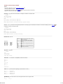
Codes needed
Manuals for all codes are available in the user manuals for Mag3D or Grav3D.
Executables
Description
Magnetics
Gravity
mag3d-gui.exe
grav3d-gui.exe
magsen3d.exe
gzsen3d.exe
The graphical user interface
Calculates sensitivities
maginv3d.exe
gzinv3d.exe
Carries out the inversion
magfor3d.exe
gzfor3d.exe
Need only if forward modelling is to be done without inversion.
gm-data-viewer.exe
- This is a mapped data viewing utility
details - introduction
1 of 2
MeshTools3D.exe
- 3D volume viewing utility, with the ability to design a mesh, construct a model, and initiate forward modelling of magnetic or gravity data
(assuming forward calculation codes are present).
Examples used in this workflow
Throughout this workflow simple examples will be used for illustration.
Description of a small scale real example, with answers to the 6 questions above ("Clarify the problem").
Download the data, models, utility code files and other details for this scenario.
Data and model for a synthetic example.
Expand All | Contract All
details - introduction
2 of 2
Setup
1. Setting up for inversion
Setup involves gathering all available information and understanding about the problem. Outcomes depend upon assumptions, and your
perception of success depends upon expectations.
Expand All | Contract All
Clarify the problem
Relations between geological or geotechnical requirements and geophysical information must be clear because model and inversion parameter
choices depend upon the context of the task. Therefore, be sure you have answers to the following questions:
1. What is the purpose of the survey and what kind of outcome is required? In particular, why do an inversion? How will it help answer the
problem?
2. How does the geologic or geotechnical question relate to geophysical properties. (Magnetic susceptibility for magnetic surveys and
density for gravity surveys).
3. What is the configuration and extent of the region of interest?
4. How deep are targets likely to be?
5. What resolution is possible given the survey configuration.
6. Also, what resolution is required for addressing the task's needs? The necessary vertical and lateral resolution may be different.
7. What details are known about the field survey, the location and the task?
Physical properties
Expectations about target and host properties must be considered, either based upon field measurements (hand or core samples) or by
considering the literature and estimates of values for expected rock types.
Magnetics
1.
2.
3.
4.
5.
How do magnetic susceptibility contrasts relate to the problem?
What are expected physical property values?
Are there measurements of susceptibility from samples or core, or from borehole logging measurements?
Are values of magnetic susceptibility "large" - ie over ~ 1.0 SI or so?
Is target likely to have remanent magnetization?
Gravity
1.
2.
3.
4.
How do density contrasts relate to the problem?
What are expected values of density?
Are there measurements of density from samples or core, or from borehole logging measurements?
Are values of density "large" - ie more than ~2.0 gm/cc or less than ~ -2.0g/cc?
Prior information
Information about the problem and the setting that already exists is important. No geophysical work is ever done completely "blind". Prior
information drives many of the decisions about how inversion will be carried out. Examples of prior information include knowledge about the
target and background rock types & magnetic susceptibilities or densities, and the location, depth, and shape of targets and structures.
There should also be as much information as possible about objects or features that could be a source of noise present in the survey area. As one
example, it may be useful to consider whether the effect of basement rocks could mask responses of features of interest.
Forward modelling
It is usually helpful to build realistic expectations by experimenting with synthetic models. This is forward modelling. It is done by generating
synthetic models which approximate expected geology, calculating data over these simplified models, inverting those data, and comparing
inversion results to the original synthetic model.
A separate page
outlines how forward modelling (magnetics) can be used to build expectations for a simple example.
1 of 1
Data
2. Data preparation
1. Introduction
Data preparation is the most important aspect of any geophysical inversion. This section explains how to prepare data and characterize standard
deviations. It also outlines what must be known or understood about the data to ensure a successful inversion.
Expand All | Contract All
2. Specifying data
Five aspects of data specification need consideration.
A) Data, types and units
General considerations (mag and grav): Data must consist of the anomaly only, with no contributions from fields caused by materials
outside the volume under the survey area. Data can be either airborne, marine, ground-based, or borehole data. Magnetic and gravity gradient
data can NOT be inverted using MAG3D or GRAV3D. Input data file formats are summarized for mag or grav data.
How much data is enough? It is not always good to include all data available. Several data points per cell (at the surface) are usually enough.
Very large data sets usually can be decimated, resulting in faster inversions (see 3. Pre-processing below).
Required and recommended processing steps: Ensure there are no gains or other factors applied by instruments, and see 3. Preprocessing
below for more comments.
NOTE that the free educational versions of MAG3D and GRAV3D permit no more than 400 data values.
Magnetic data
Magnetic data must be the residual magnetic intensity after diurnal variations and regional effects are removed. Usually data are total field
anomaly data, but multi-component data (X, Y, or Z component data) can be inverted.
Units of data being inverted using MAG3D must be nanoTeslas.
The local magnetic field: Correct inclination, declination and total field strength (I,D,F) for the latitude, longtitude, elevation and date of the
survey must be known correctly. These are parameters {incl, decl, geomag} in the mag data files. If a total field survey was carried out then
the input file parameters {aincl, adecl} are the same as {incl, decl} because measurements are of anomalous fields "projected" onto Earth's
field. If the field survey was carried out with an oriented instrument the {aincl, adecl} represent the orientation of the instrument's orientation.
For example, using a vertical component fluxgate magnetometer, {aincl, adecl} = {90,0}.
Multi-component (often borehole) data, consisting of magnetic field measurements in more than one direction (collected with instruments
such as flux-gate magnetometers that have specific orientations), require orientation details for each datum. See the summary of
multi-component data specifications .
If there are variations of (I,D,F) within the data set (for example, if two portions of the data set were gathered several decades apart), data must
be rotated so they all appear as if collected together. The reason for this is that there is only one place for defining total field strength in the data
file (on the first line - see parameter "geomag" in the mag data files).
Gravity data
Gravity data must be corrected for drift, latitude, elevation, and "host rock density". In other words, required data reductions are (i) instrument
& tidal drift, (ii) latitude, (ii) free air, and (iv) Bouguer corrections. Also, topography must be included as part of the inversion, unless total
topographic relief is less than one cell thickness. For input file specifications, see the grav input files summary.
Units of data being inverted using GRAV3D must be milliGals.
B) Positioning, elevation and coordinate systems
For each datum, the location and elevation of the sensor (above topography for ground/air data, below for borehole data) must be given
as x, y, z in metres.
Coordinate systems used for data, topography and the model (i.e. the mesh - see Chapter 3, Defining the model) must be consistent.
Location-specific processing or information, like the orientation of the inducing magnetic field, must also be transformed to the coordinate
system of the data and model.
Inaccuracies in location must be accounted for in the assignment of standard deviation.
Make sure no data are below topography. For airborne data, both topography-draped and constant-height surveys can be used as long as all the
location information is available. If elevation information isn't available then the elevations can be estimated by adding the nominal flight height
to terrain elevations at each location.
C) Gridded data
Data are often gridded in order to provide station locations that are regular, or to reduce the number of data. Sometimes only gridded data are
available. However, for inversion, it is recommended to NOT use gridded data, but rather to use the original data with the correct associated
locations. This is because gridding calculates a data value at a location rather than using the one that was actually measured. There are many
1 of 3
Data
different gridding methods, and different data sets will be produced by each method.
When dealing with data (airborne or ground) collected over topography, gridding can be even more detrimental because the gridding algorithm
may not account for the different elevations at which the data where collected.
If is it necessary to reduce the number of data, it is advisable to down-sample or decimate the data along the line that it was collected. See
Preprocessing below.
NEEDED: Examples of problems caused by gridding.
D) Viewing data and QC
To examine data and assess quality (Quality Control, or QC), use the data viewing program gm-data-viewer
control include asking the following questions:
. Some basic aspects of quality
Who was running the survey that day? Is there a correlation between operator and sensor height? Is this consistent?
Were clearly erroneous data removed.
What is the range of the data?
Has the regional field been removed? Data values far from subsurface zones with non-zero susceptibility should be close to 0.0nT. Even if
there are features that we would usually consider as noise (magnetic culture such as buildings, drill-holes, and power-lines), the signal
they produce is measured by the sensor and will be accounted for in the inversion.
E) Topography
If topography is being included then it should be provided for the whole area being considered and with a data density appropriate for both the
level of discretization and for the roughness of topography (ie. at least one value per mesh cell).
Topography as specified using XYZ values, and gridded topography is not necessary. A good dtm or dem (digital terrain map or digital elevation
model) can provide topography. See the grav3d
or mag3d
manuals for details about how to specify topography in relation to the model's
mesh.
3. Pre-processing
While not exhaustive, this list summarizes the types of processing that can be applied prior to inverting magnetic data.
Recommended procedures for magnetic AND gravity data are:
Regional field must be removed as accurately as possible. Potential field data usually have regional, or long wavelength, components
that are produced by geologic features outside the region of interest. These regional features should be removed prior to inverting the
data. There are several methods outlined in the "regional removal" section of Chapter 6, Advanced techniques.
Upward continuation to a height of half the thickness of the shallowest cells will remove near surface effects without degrading the data
too much. Thus upward continuation is a recommended procedure for ground based data.
Decimate: If there are more than a few data points over every cell at the surface of the model, you may consider down-sample the data
set along survey/flight lines. This is much preferred over gridding, as explained above. Decimating can be carried out within
gm-data-viewer .
Cropping: The data can be cropped to include only the anomalies resulting from the features that are to be modelled. When anomalies in
the data are not completely included, the resulting models are not well defined in these regions. Cropping can be done within
gm-data-viewer .
Duplicates: No duplicate locations are permissible in the data file. The data should have unique locations for each measurement of the
magnetic field. If duplicate data points are found then some data could be removed or an average value used.
Decorrugation: Decorrugation or flight-line effects should be removed if possible, or accounted for when defining standard deviations.
Gravity data: Gravity data reductions are required. See Section 2A) above, "Data, types and units".
Magnetic data: Diurnal variations of the Earth's magnetic field must be removed through comparison with data from a local, stationary
reference or base station.
4. Procedures that are NOT recommended
Prior to inversion, do NOT use any processing steps commonly applied to mapped data which make it easier to interpret or highlight map
features. Inversion requires generating predicted data, and comparing those predictions to measurements. Most forms of filtering make this
comparison difficult. Specifically, procedures that are NOT recommended include the following:
Downward continuation should NOT be necessary (see also remarks about levelling below).
Reduction to the pole is not recommended before inversion because of the limitations of this process at some latitudes. However it can
help merge data sets acquired at different times.
Gridding: discussed under "Specifying Data" above.
Levelling: Levelling is usually done to adjust data collected at different elevations so the map is smooth across boundaries of adjacent
data sets. Therefore, for reasons that are similar to gridding, levelling is not necessary so long as true elevations of every datum are
known. If data sets were gathered a very different dates, then one data set may need to be adjusted so the ambient field is the same for
all data.
Bandpass filtering: Usually not necessary unless removing regional signals. Note that it is not helpful to have features in data sets
caused by structures smaller than surface cells. However, decimation is better than filtering because it does not modify data values.
Gradients of data can not be inverted THEREFORE vertical, horizontal, second vertical, analytic signal, and all other derivative filtering
techniques must not be employed prior to inversion.
All data transformation process such as pseudo-susceptibility or pseudo-gravity transforms must not be used.
2 of 3
Data
5. Characterize data reliability (noise or errors)
Data and location measuring devices are very precise but real data are never as accurate (i.e. "conforming exactly to fact") as suggested by
instrument specifications because surveying in the field is complex and subject to many sources of error. Standard deviations for data must be
specified (last column of the input data file) so that a suitable degree of misfit can be used in the inversion.
Sources of error include processing inaccuracies or assumptions, positioning errors, and errors in accompanying information such as the
topography or inducing field parameters. Furthermore, due to limitations of the model discretization and topographic representation, small
geologic features will not be accurately represented in the forward modelling process. As a result, it can not be expected that the data will be
perfectly reproduced from a model produced by inversion.
Errors in positioning (uncertainty in (x,y,z) location of the sensor for each datum) contribute to errors, so if there are (x,y,z) locations that are
particularly uncertain, corresponding data must have larger standard deviations assigned.
Recommended practice: Errors are rarely measured in the field, so the following guidelines apply (note that errors are usually assumed to be
random and Gaussian):
Standard deviations can be specified using a percentage of the datum plus a minimum (or "offset") value in units of nT or milliGals.
Unless specific information is known, or obvious noisy data can be identified, it is usually assumed that all data from the same survey have
the same accuracy so the same standard deviation can be used for all.
How much error?
With current data accuracies and modelling limitations, values of standard deviations are generally assigned between 0.05 and 1 nT
for magnetic surveys, or on the order of 3 to 5 times the gravimeter's sensitivity for gravity surveys. This depends on the scale of
the data coverage and the accuracy of the sensor and location information.
A larger value for standard deviation would be needed for less reliable data.
Data from older surveys may be less accurate and therefore need larger standard deviations.
If the data set is being down-sampled, it may be possible to use neighbouring data to help define a standard deviation. This has not
been studied rigorously, but seems like a good idea.
Three ways to specify error information are:
1. Supply standard deviations for data directly in the data file (units of nT or milliGals).
2. The gm-data-viewer program
can generate standard deviations for all data based on user supplied values. Point to a datum with
the mouse and press <SHIFT - Right Button>.
3. Details in mag or grav data file specifications.
Supply standard deviations in the same units as the data.
More explanation
about why standard deviations must be supplied is given on a separate page.
Expand All | Contract All
3 of 3
3. Defining the model
MAG3D and GRAV3D both use a 3D model
susceptibility (or density) for each cell.
of the earth consisting of 3D rectangular cells of fixed sizes. Inversion determines values of
High resolution (many small cells) is often desirable. However, survey configuration will limit resolution. It is hard to image features smaller
than the largest measurement spacing (usually line spacing).
Also, the computing system limits the number of cells. A matrix the size of [total No. data X total No. cells] must be stored in memory.
Two files define the model; a mesh file (mag grav ) defining 3D rectangular cell geometry (sizes and locations), and a model file (mag grav
), listing values of susceptibility or density for each cell. It is advisable to start with a mesh built automatically by the MAG3D or GRAV3D GUI .
Adjustments can then be made to that model if necessary.
The default mesh and models
The GUI for MAG3D or GRAV3D will build a mesh after asking you to supply an initial cell size. A good starting cell size is usually roughly 1/25 of
the lateral extent of data. This will produce a first-pass inversion which is useful for checking that all the files and parameters are working, even
if it is not used as a final inversion. The resulting mesh will have the following characteristics.
The thickness of cells will be half their width (eg 50m x 50m cells will be 25m thick) in the main region of the model.
Depth of the main zone will be 1/4 the lateral extent of the survey area. An equal thickness will be added using cells that are twice as
thick.
Three padding cells will be added on all 4 sides of, and below, the model, with cell dimensions increasing outward.
Topography will be approximated using rectangular cells. A topography file (mag grav ) must be included if the survey area is not flat.
Model produced
for a synthetic magnetics example.
Specifying custom models
Always start by carrying out an initial inversion using a default mesh.
Also, if the mesh is large (> 100,000 cells) consider starting with a mesh that is coarser than default in order to make sure the data is inverting
well before starting time consuming inversion runs.
Guidelines for custom mesh design are given separately.
Related information:
Mesh
, model
& topography
file formats.
Note the free, educational versions of MAG3D and GRAV3D allow for models with no more than a total of 12,000 cells. (eg; a 25x25x19 mesh
would be OK).
Defining the model
1 of 1
4. Basic inversions
- Sections 1 through 4 on this page describe how to set up a basic inversion.
- Sections 6 and 7 describe how to check results.
- Numbered points refer to the MAG3D GUI image . The GRAV3D GUI is effectively identical.
- See the MAG3D GUI manual
for details about each input field of the user interface.
- Starting with a default inversion is recommended because it helps determine how to adjust the process to obtain optimal results.
- Refer to Introduction, Best practice for general recommendations about running the codes.
NOTE: one inversion is never enough: After a default inversion has been run, adjustments to inversion parameters should be employed to
refine the resulting model. See Chapter 5, Subsequent Inversions.
Expand All | Contract All
1. Input files
The following input files must be prepared.
Numbered points refer to the GUI image .
1 - Observations file: The data.
See Chapter 2, Data preparation.
3 - Mesh file: The mesh; i.e. model specification.
See Chapter 3, Defining model characteristics.
5 - Topography file: optional. Topography over the survey area is specified in a simple text file containing elevations at x/y locations.
See Chapter 2, Data preparation.
All other parameters are explained in the next three sections.
2. Setting model objectives
Recall numbered points refer to the GUI image .
2 - Depth / distance weighting: Counteracts the natural decay of potential fields. More details .
7 - Bounds: Optional values or files specifying upper and lower bounds on recovered property values for seach cell. Default values are
(upper,lower)=(0.0,1.0) SI for magnetics and (upper,lower)=(-2.0 to 2.0) g/cc for gravity. (Recall that models from gravity data are density
contrasts). Specifying non-default bounds is an "advanced" technique - see Chapter 6.
8 - and 9 - Initial and reference models: both are optional files or values. Click here for a short explanation of initial and reference models.
Default: the program sets initial and reference models to 0.0 (S.I. or g/cc).
Value: specify a value (units of S.I. or g/cc) to be used as an initial and/or reference halfspace model.
Model files: You must specify a model that using exactly the same mesh as the inversion.
For more on using reference models see Chapters 5 and 6.
10 - Alpha / Length scales - coefficients in the model objective function that set the relative importance of smoothness vs closeness to a
reference. Details .
Weighting matrix - (not the same as distance weighting) optional and advanced. Access to this facility is not provided within the GUI. See the
MAG3D Software manual , Chapter 4 Elements of MAG3D, section w.dat.
3. Misfit, and tradeoff options
Recall numbered points refer to the GUI image .
6 - Mode: GCV, Chifact or Constant tradeoff.
- GCV (Generalized Cross Validation) is computing intensive but finds it's own tradeoff parameter. Using a GCV inversion to help find an optimal
misfit is outlined elsewhere .
- Chifact; Changing the Chifact parameter adjusts the acceptible misfit between observed and predicted data for the whole data set. As noted
immediatly above, the GCV mode can help find an optimal value. A separate page illustrates the effects of adjusting Chifact in a 2D example.
- Assigning a constant tradeoff is rarely used, but might be appropriate if previous work has shown a specific value to be suitable. This is an
"advanced" technique.
4. Compressing the size of the problem
Sensitivity: The inversion process is solved in two stages with a preliminary calculation of the sensitivity matrix followed by the actual inversion.
The sensitivity calculations are "compressed" using wavelets, thus speeding up the inversion.
GUI item 4 - Wavelet compression: The level of wavelet compression is set via a threshold which controls the accuracy of the sensitivity
matrix when it is not compressed. These parameters are rarely changed as the defaults are usually adequate.
Further explanation is provided in notes about sensitivity , including remarks about Recognising matrix compression problems.
Basic inversions
1 of 2
5. Running the inversion
Running an inversion: Save setup parameters before using the "Run" button to initiate the inversion. See "Introduction - Best Practices" for
guidelines.
6. Assessing the algorithm's outcome
The inversion estimates models using well-defined optimization criteria. Since the user is in control of those criteria, the inversion progress
should be monitored to ensure the outcome is reasonable. Three aspects should be checked.
1. Two log files provide details about the algorithm's progress.
- File magsen3d.log (or gzsen3d.log for gravity inversions) summarizes inputs and outcomes of calculating sensitivity. A problem with
input files will be indicated by an error message near the end of this file.
- File maginv3d.log (or gzinv3d.log for gravity) summarizes progress of the inversion algorithm.
Details about MAG3D and GRAV3D log files are in the MAG3D Software manual
Chapter 6, Log file example.
, Chapter 5, Running programs, section "Log files", and
2. Assessing misfit: There are two aspects:
- Predicted data generated from the model should be visually compared to measured data. (details )
- The final value of misfit (first column, last row, at the end of file maginv3d.log (or gzinv3d.log)) should be consistent with the number
of data and the value of Chifact. If GCV mode was used, this value should be within roughly 0.5N - 5.0N (where N is the number of data).
3. Character of models: The model itself should be observed and considered, particularly in terms of whether it is geologically reasonable,
and compatible with all prior knowledge. This is a complex task which benefits from experience, and interaction with other professionals
involved in the task (geologists, exploration specialists, etc).
7. Display the resulting model
To view the model from the GUI, the meshtools program (MeshTools3D.exe) must be in the same directory as other inversion executable
programs. There is a separate manual
for MeshTools3D. When viewing MAG3D or GRAV3D inversion outcomes, some initial considerations
include:
1. Are the physical property min / max values (MeshTools3D Options menu) appropriate for emphasizing desired details within the model?
2. Slicing reveals all values of model cells on one slice through the volume.
3. Isosurfaces provide a visual impression of the volume containing susceptibility (or density) values that are greater than a chosen cutoff
value.
4. Choices of min/max colour scale and isosurface cutoff have a significant affect upon subjective visual impressions, and therefore on
what will be interpreted about geology.
Expand All | Contract All
Basic inversions
2 of 2
5. Subsequent inversions
A single inversion is never enough for several reasons, given here . Note that when adjusting parameters to explore various inversion outcomes,
it is safest to change only one parameter at a time.
This page outlines commonly used modifications to inversion parameters, while more advanced procedures are given in Chapter 6. The first
approach outlined below is a good way to begin, but any of the approaches to finding alternate models may be suitable.
Expand All | Contract All
A. First alternate model
If a GCV mode result is obtained, a good first alternative model can be obtained by changing the misfit as outlined here .
Another possible first alternate model could be obtained by adjusting the smoothness in different directions as outlined in the example under D.
below.
B. Adjusting misfit
The allowable discrepancy between measurements and predicted data (ie the target misfit) can be adjusted by changing the Chifact parameter.
When noise on data is in fact random and Gaussian the theoretically correct value for Chifact is 1. To modify the degree to which predicted data
are required to match measured data, change Chifact as follows:
Increasing Chifact "loosens" misfit, yielding a model that generates predicted data that look less like data with their errors.
Decreasing Chifact "tightens" misfit, resulting in more complex models with predictions that look closer to data, including their errors.
A separate page illustrates in 2D the effect of employing a range of values for Chifact.
Choosing the best misfit for any given data set is not always straightforward. However, one approach, using the GCV mode is outlined here .
C. Changing the reference model
In section (9) of the MAG3D (or GRAV3D) GUI , selecting "Default" causes the program to use a reference model consisting of a uniform earth
with a constant physical property value of 0.0 S.I (or 0.0 g/cc).
Modifying the reference model is a powerful tool for exploring which regions of the model are reliably defined by the data. However, most
inversions are done assuming that "host" or non-target materials have susceptibility or density contrast of zero because regional effects have
been removed from the data. Therefore, specifying a reference model which is mainly non-zero should be done cautiously, and only when there
is very good knowledge about the extent of the non-zero regions and their values. Consequently, unlike when using DCIP2D , changing the
reference model in MAG3D or GRAV3D is considered an "advanced" process. See workflow Chapter 6.
D. Adjusting "Alpha" parameters
In section (10) of the GUI , the so-called
coefficients, or equivalently the length scales, can be adjusted to control what kinds of model
characteristics are emphasized. The following example illustrates this procedure:
Check the default values for length scales Le, Ln, Lz near the top of the inversion log file (maginv3d.log or gzinv3d.log). They should be
100,100,100.
Change one of these to 1. This will de-emphasize smoothness in the corresponding direction.
Save this new set of inversion parameters to a new subdirectory, and run the new inversion.
Inspect the outcome, and compare to the default model by opening a second MeshTools window with the default model. (Check the
MeshTools manual for features that help compare different models.)
See an example of carrying out this procedure.
The similarities and differences can be used to help answer some of the issues discussed on the justification
Additional explanations about
page.
coefficients are provided here .
Expand All | Contract All
Subsequent inversions
1 of 1
6. Advanced techniques
Introduction
Acceptable results usually can be obtained using basic procedures covered in previous sections. However, there are many advanced ways of fully
exploiting the power of adjustable model objective funtions, misfit criteria and tradeoff procedures. Also, some situations will require special
attention to data preparation. The following suggestions can be pursued to further refine the models, or to explore more fully the range of
potential models.
It is also desirable to incorporate as much prior information as possible, and this can involve some advanced techniques.
Expand All | Contract All
1. Refining the misfit criteria
Adjusting Chifact (as outlined in Chapter 5) loosens or tightens the misfit criterion in a global sense. However, if individual data points can be
considered less (or more) reliable than other data points, then standard deviations for those datum values can be individually adjusted.
In the data viewer , hold the SHIFT key while clicking on the datum with the right mouse button, then you can assign a value specifying the
standard deviation for that individual datum, in units of nT (or g/cc).
Increasing this value for a single data point allows the inversion program more flexibility to find a model that reproduces that datum less closely
than all other data values.
2. Advanced use of reference models
NEEDED: Advanced workflow with an example is required.
3. Incorporating bounding constraints
GUI section (7) facilitates specification of either (i) global upper and lower bounds on the value of susceptiblity or density in all cells, or (ii)
specific upper and lower bounds for each model cell individually.
Default upper and lower bounds for MAG3D are 1.0 and 0.0 (S.I. units) respectively, and for GRAV3D, -2.0 and 2.0 g/cc respectively.
For magnetic inversions, specifying a global lower bound above 0.0 is not commonly done because targets are usually susceptible zones in
essentially non-susceptible host rocks.
Specifying upper and lower bounds for specific cells or regions is done using a special (optional) file containing upper and lower bounds for every
cell. The file has a format similar to a model file except that there are two values for every cell instead of only one. It must be prepared using the
same mesh that is being used in the inversion. See Chapter 4, "Elements", the Bounds section, of the MAG3D
or GRAV3D
software manuals.
NEEDED: example(s) of employing bounds (gravity?).
4. Including a weighting function
NOTE: the MAG3D and GRAV3D GUIs do not include an option for incorporating weighting matrices (not the same as depth weighting). This must
be done using an inversion input file called with the inversion program (maginv3d.exe or gzinv3d.exe) from the command line.
Incorporating weighting into the inversion is similar to adjusting the model objective function using
parameters, except that each cell can be
modified individually. Weightings are applied to penalize smoothness in the X- Y- or Z-direction, or closeness to the reference for any cell in the
model. Here are specifics points:
If smoothness is penalized for some cells, minimization of the objective function will concentrate on achieving a result that is close to the
reference with less concern for smoothness in those cells.
If closeness to a reference is penalized for some cells, minimization of the objective function will concentrate on achieving a result that is
as smooth as possible, with less regard for how close to the reference model the result is in those cells.
Weighting files are similar to model files except that all three weightings are in one file. See the description of file "w.dat" in the software
manuals, Chapter 5, "Running programs", for MAG3D
or GRAV3D .
Here are examples of applying weighting. A 2D example is used because it is easier to illustrate the effect. 3D results will be analogous.
Of all the ways in which model objectives can be adjusted, incorporating weighting into the objective function produces the most subtle effects. It
is not common to make extensive use of this capability, but it does provide an opportunity to explore "model space" more carefully.
5. Removing regional effects
Potential field data usually have regional, or long wavelength, components that are produced by geologic features larger than, and/or outside,
the region of interest. These regional features should be removed prior to inverting the data.
One common method involves using a curve-fitting algorithm to find a best-fit nth-order polynomial ("n" chosen by experience or trial-and-error).
Then that polynomial surface is subtracted from the data set, ideally leaving only the contributions from anomalies under the area of interest.
A two-step inversion can also be employed, first making use of a large scale regional data set, then working with the local area of interest. This
procedure is outlined in more detail on a separate page.
Advanced techniques
1 of 2
Even after regional removal (by whatever means) there may still be non-zero anomalies near survey area boundaries. In that case, the model's
mesh must be augmented with padding cells, and the recovered values of susceptibility in those padding cells ignored during interpretation.
NEEDED - an example.
6. Other advanced topics
IMPORTANT: Other than upward continuation, data processing steps that change the values or locations of data points should be avoided if
possible. This is because success depends upon accurate forward modelling, and any processing would have to be accuratly reproduced in the
forward modelling algorithm. See Chapter 3, Data Processing, Section 3, Pre-processing for more details.
Other topics that can be considered "advanced" are listed here. Grayed out points are incomplete.
1. High susceptibilities: The presence of materials with susceptibilities greater than roughly 2 (S.I.) causes demagnetization effects, and
the forward modelling problem becomes very non-linear. Such situations are not solvable using MAG3D. Evidence that this might be a
problem includes ...
NEEDED: details here.
2. Modifying depth (or distance) weighting: when and how.
3. Incorporating borehole and surface physical property sampling information. NEEDED: pointer to workflow for this.
4. Forward modelling: NEEDED: workflow for generating models, calculating data, then inverting. Via a simple step-by-step with the
"mystery" model??
5. Large Areas: NEEDED: how to carry out tiling, including effects of different inducing field parameters.
6. Not clear about notes from N.P. on Curie Point ??
Expand All | Contract All
Advanced techniques
2 of 2
7. Using inversion results
This page identifies several key aspects of using inversion results. Note however that there is no substitute for professional experience.
In general, remember that interpretation of geophysical work is a two step process, and that the second step can not be done until the first is
satisfactorily accomplished.
1. First a model is produced which gives one feasible distribution of the relevant physical property;
2. Then this physical property model is interpreted in terms of geological or geotechnical parameters that are directly relevant to the project.
Chapter 5, "Subsequent inversions", explains why you must base your interpretion on several inversion results. The importance of this point can
not be emphasized enough. The rest of this page provides some guidance on aspects of interpretation which commonly raise questions or cause
confusion.
Expand All | Contract All
1. Smooth models
One significant aspect of most current inversion codes is that they are designed to produce "smooth" models. The reason for this is explained on
a separate page .
Identifying structural boundaries may be challenging using smooth models. However, at any particular site, the physical property value used to
represent a boundary between two geologic units is likely to be consistent. Therefore, even a single point of alternative information, such as the
intersection of rock units in a borehole, can be all that is needed to interpret a smooth model in terms of structural features.
Forward modelling is a useful way of gaining insight about how specific structural configurations might be imaged using data and inversion
techniques that are available. This was mentioned in Chapter 1 "Setting up for inversion", and a separate page outlines how forward modelling
can be used to build expectations for a simple problem.
2. Method specific topics
NEEDED:
Characteristics of susceptibility models obtained with surface or borehole data. See mag3d manual and Li, Oldenburg, 2000 (geop65)
Effects of erroneous application of the Bouguer correction.
Effects of not properly removing the regional field.
3. Survey design
The most efficient field surveys are those that provide only enough data to characterize the earth with detail sufficient for the requirements. One
useful technique for establishing the necessary coverage and accuracy for any particular situation is to calculate possible data sets based upon
suitable synthetic models and then invert the results. The work can be repeated to establish a suitable quantity and distribution of data points.
NEEDED? example (perhaps from M Roach)?
4. Other advanced topics
Some other topics for which notes are being compiled include:
Spotting depth weighting issues.
Understanding distance weighting when borehole data are used.
Expand All | Contract All
Using inversion results
1 of 1
pitfalls
8. Pitfalls and challenges
Items on this page identify situations that may be challenging for various reasons.
Remanence artifacts may be occuring if a 'move-out' effect is evident, or if the solution can not converge. This is one situation where you need
a reasonable expectation of the results so you can see when things go wrong. Note also that if there are surveys gathered at very different dates
(i.e. with different inducing fields), then if different results are obtained from each of the surveys it is possible remanence is present.
Incorrect inducing field direction: It may be difficult for the algorithm to converge, or the resulting model may appear very "un-geological".
Noisy models at depth: This can be caused by over-fitting the data, or there may be remanence effects.
High values in padding cells: This is most often caused by some regional signal that is still present. Regional signal is caused by features
larger than (or outside) the zone below the survey area.
Combining data from surveys gathered at different elevations: This should be possible with little extra effort so long as the two data sets
are correctly characterized.
Severe topography: Severe topography can cause artifacts owing to the difference between real topographic relief and the rectangular cell
approximation of topography. Also, will a survey that samples more in 3D (extreme terrain) define the subsurface better than one that is run at a
single height? This is a good question, and one worth investigating experimentally.
Linear artifacts in the model which seem to repeat at regularly spaced intervals: This could be caused by matrix compression being set
too high. Further explanation is provided in notes about sensitivity .
NEEDED: special aspects of gravity work - errors in data reduction (such as improper density for Bouguer correction), effects of not carrying out
appropriate corrections ... others?
NEEDED: pros and cons of upward continuation - examples?
Other topics that might find a place in this workflow at a future date:
Running parallel processing versions of MAG3D and GRAV3D.
Viewing / using the sensitivity matrix.
1 of 1
Summary of file formats for MAG3D
NOTES:
- For gravity data files, see the gravity data formats file.
- All files are ASCII text files.
- For details about each file see the MAG3D
user manual (section 4 "Elements").
- Data are in units of nano-Teslas.
obs.mag: Input data. See the manuals for examples of surface or borehole data.
! comments ... !
Incl Decl geomag
Aincl Adecl idir
ndat
E1 N1 Elev1 [aincl1 adecl1] Mag1 Err1
E2 N2 Elev2 [aincl2 adecl2] Mag2 Err2
:
Endat Nndat Elevndat [ainclndat adeclndat] Magndat Errndat
obs.loc: used to specify the inducing field parameters, anomaly type and observation locations for forward modelling. See the manual
examples of surface or borehole data.
for
! comments ... !
Incl Decl geomag
Aincl Adecl idir
ndat
E1 N1 Elev1 [aincl1 adecl1]
E2 N2 Elev2 [aincl2 adecl2]
Endat Nndat Elevndat [ainclndat adeclndat]
fdmesh.dat: Mesh file
NE, NN, NV
NE NN NV
E0 N0 V0
E1
E2 ...
N1
N2 ...
V1
V2 ...
E0, N0, V0
ENE
NNN
VNV
Number of cells in the East, North, vertical
directions respectively.
Coordinates, in meters, of the southwest
top corner, specified in (Easting, Northing,
Elevation).
En
Cell widths in the easting direction (from W
to E).
Nn
Cell widths in the northing direction (from S
to N).
Vn
Cell depths (top to bottom).
topo.dat: Topography
! comment
!
npt
E1 N1 elev1
E2 N2 elev2
Enpt Nnpt elevnpt
model.sus: The model file - susceptibility values for each cell
sus1,1,1
sus1,1,2
:
sus1,1,NV
sus1,2,1
:
susi,j,k
:
susNN,NE,NV
w.dat: User specified special weightings (values between 0 and 1).
W.S1,1,1
W.E1,1,1
W.N1,1,1
W.Z1,1,1
...
...
...
...
W.SNN,NE,NV
W.ENN,NE-1,NV
W.NNN-1,NE,NV
W.ZNN,NE,NV-1
BOUNDS.dat: cell values of the lower and upper bounds on the sought model.
lk1,1,1
File formats
uk1,1,1
1 of 2
lk1,1,2
:
lk1,1,NV
lk1,2,1
:
lki,j,k
:
lkNN,NE,NV
File formats
uk1,1,2
uk1,1,NV
uk1,2,1
uki,j,k
ukNN,NE,NV
2 of 2
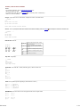
Summary of file formats for GRAV3D
NOTES:
- For magnetic data files, see the magnetic data formats file.
- All files are ASCII text files.
- For details about each file see the GRAV3D
user manual (section 4 "Elements").
- Data are in units of milliGals.
obs.grv: Input data. See the manuals for examples of surface or borehole data.
! comments ... !
ndat
E1 N1 Elev1 Grav1 Err1
E2 N2 Elev2 Grav2 Err2
:
Endat Nndat Elevndat Gravndat Errndat
obs.loc: used to specify the observation locations for forward modelling. See the manual
for examples of surface or borehole data.
! comments ... !
ndat
E1 N1 Elev1
E2 N2 Elev2
Endat Nndat Elevndat
fdmesh.dat: Mesh file
NE, NN, NV
NE NN NV
E0 N0 V0
E1
E2 ...
N1
N2 ...
V1
V2 ...
E0, N0, V0
ENE
NNN
VNV
Number of cells in the East, North, vertical
directions respectively.
Coordinates, in meters, of the southwest
top corner, specified in (Easting, Northing,
Elevation).
En
Cell widths in the easting direction (from W
to E).
Nn
Cell widths in the northing direction (from S
to N).
Vn
Cell depths (top to bottom).
topo.dat: Topography
! comment
!
npt
E1 N1 elev1
E2 N2 elev2
Enpt Nnpt elevnpt
model.den: The model file - density contrast (gm/cc) values for each cell
den1,1,1
den1,1,2
:
den1,1,NV
den1,2,1
:
deni,j,k
:
denNN,NE,NV
w.dat: User specified special weightings (values between 0 and 1).
W.S1,1,1
W.E1,1,1
W.N1,1,1
W.Z1,1,1
...
...
...
...
W.SNN,NE,NV
W.ENN,NE-1,NV
W.NNN-1,NE,NV
W.ZNN,NE,NV-1
BOUNDS.dat: cell values of the lower and upper bounds on the sought model.
lk1,1,1
lk1,1,2
:
lk1,1,NV
lk1,2,1
:
File formats
uk1,1,1
uk1,1,2
uk1,1,NV
uk1,2,1
1 of 2
lki,j,k
uki,j,k
:
lkNN,NE,NV ukNN,NE,NV
File formats
2 of 2
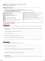
Checklist
Inversion workflow: 3D magnetics / gravity
A printable checklist or worksheet
Preparing for inversion
1.
2.
3.
4.
Don't skip preliminary steps - they affect decisions later during the flow of work.
This is an outline only. The complete workflow should be studied if you are not experienced with the codes.
Have you read about "Best practices" in the introduction?
Check Relevant assumptions via the following checklist:
1. Assumptions for surveys:
2. Expectations for 3D inversion results:
Known topography or assumed flat.
information becomes less reliable gradually as depth increases.
Suitable problem (not objects or layers).
resolution becomes coarser gradually as depth increases.
Have regional components of data been removed?
MAG3D:
Susceptibilities assumed < 1.0 S.I. (roughly).
I, D, F are known and constant for the area.
GRAV3D:
models are smooth and close to a reference model.
true min/max values are probably smaller/larger than recovered
values.
many models are possible, but all will reveal important features.
Data are corrected Bouguer anomalies without the "topographic
correction".
Recovered densities will be density contrasts .
1. Setting up for inversion
Clarify the problem
1. What is the purpose of the survey and what kind of outcome is required? In particular, why do an inversion? How will it help answer the
problem?
2. How does the geologic or geotechnical question relate to geophysical properties. (Magnetic susceptibility for magnetic surveys and density
for gravity surveys).
3. What is the configuration and extent of the region of interest?
4. How deep are targets likely to be?
5. What resolution is possible given the survey configuration?
6. What details are known about the field survey, the location and the task?
1.
Physical properties
1. How do susceptibility (or density) contrasts relate to the problem?
2. What are expected physical property values?
3. Are there measurements of property values from samples or core, or from borehole logging measurements?
4. (Magnetics only: Are there likely to be remanent magnetization effects?)
5. Prior information:
A) Summarize what is already known about the target, background rock types & physical properties, and the locations, depths, and shapes
of targets and structures.
1 of 3
Checklist
B) Summarize possible objects or features that contribute to result but which are not part of the target.
6. Forward modelling:
Consider generating synthetic models which approximate expected geology, calculating data, inverting, and comparing results to the
original synthetic model.
2. Magnetic or Gravity data preparation
The following check list should be followed in order.
1.
MAGNETIC Data have been corrected to remove ambient field.
2.
GRAVITY data are Bouguer anomaly data without topography correction.
3.
Regional effects should be removed, either by subtraction of a polynomial or using a two-step inversion procedure involving a large
regional data set. See Advanced Techniques.
4.
Only an appropriate amount of data should been kept. Decimate, and avoid gridding if possible.
5.
Are raw data in the correct units (nT or millGals)?
6.
No data processing should have been applied - see work flow for do's and don'ts regarding data processing.
7.
Are positions and elevations (topography) in units of metres?
8.
Specify standard deviations uniformly for all data, and assign special values to data points that are noiser than most.
9.
View data after preparation to ensure the data set is good.
10.
11.
If there is topography, generate a topography file.
If you are working with synthetic data generated by forward modelling, add noise to the data (within the data viewing program).
"Perfect data" should never be inverted.
3. Defining the model
1.
2.
Start by asking the Graphical User Interface to build a 3D mesh based upon the data and topography files.
Adjust this if necessary (rarely the case) following guidelines in the workflow. Specifying cells that are smaller than half the distance
between stations is rarely useful.
3.
Add padding cells around and below if anomalies extend to edges of the data set.
4.
If the mesh is "hand made", ensure the mesh handles topography properly.
4. Basic (first) inversion
1.
2.
Specify necessary mesh, data and topography files.
Choose misfit and tradeoff options for a first inversion. GCV is a good choice for smaller problems; Chifact=1 is a good choice if errros
have been specified properly, and they are indead Gaussien.
3.
Specify default model objectives for a first inversion (default for initial & reference models, alpha's, and weighting).
4.
Leave wavelet compression at default values.
5.
6.
Save each inversion setup to a new subdirectory, under the project's root. Organize work using directory names rather than file
names.
Run the inversion.
7.
Display the model.
8. Assess the algorithm's progress:
a.
Inspect the model. Are there any surprises?
b.
Inspect predicted data and the data misfit map.
c.
Inspect the key components of the log file.
5. Subsequent inversions
1.
Never interpret geology based on one inversion alone.
2.
Adjust objectives (via Alpha or length scale parameters, or based on GCV result) and invert for a first (simple) alternative model.
3. Alternatives for adjusting the inversion outcome:
a.
Consider adjusting misfit.
b.
Consider adjusting closeness-to-reference or smoothness.
c.
Consider adjusting the reference model.
d.
Consider specifying upper and lower bounds.
6. Advanced techniques
2 of 3
Checklist
1.
2.
3.
4.
5.
6.
7.
Refine the misfit criteria (for specific data points if necessary).
Consider more complicated reference models.
Incorporate upper and/or lower bounds for recovered values.
Adjust model objective function (alpha or length scale) parameters.
Include weighting if appropriate.
Removal of regional effects via a two-stage inversion procedure is discussed in the workflow.
Does this project have other special considerations?
7. Using inversion results
1.
Understand why models are smooth, and account for this in interpretations.
2.
Ensure topography is properly accounted for.
3.
Be sure to interpret geology based upon several inversion models.
8. Pitfalls - potential probelms
There are several aspects of magnetic and gravity surveying that can make interpretation of inversion results interesting:
1.
2.
3.
4.
5.
6.
7.
Effects of remanence will cause incorrect models but remanent magnetization can not be discovered from survey data alone.
If the incorrect inducing field is specified results will be wrong.
High resolution features at depth are likely caused by overfitting the data.
Significant features within padding cells suggests that regional effects were not properly removed. Regional
Consider possible problems caused by severe topography.
Linear artifacts in the model may be caused by overly severe compression.
Are there any other possible sources of difficulty?
3 of 3