Download Program Termination Proofs

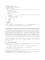
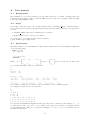
Program Termination Proofs
Tal Milea
[email protected]
Under the supervision of Prof. Hans Zantema
January 19, 2012
Abstract
Proving termination of programs is an undecidable problem. In this work we provide a sound
method for proving the termination of a certain class of programs by using the power of linear
programming tools. We handle while-loops with a simple loop condition where the assignment of the
variables is nondeterministically-chosen out of a set of possible linear assignments. We implement a
simple efficient tool for proving termination and compare it with other existing tools.
1
Introduction
Proving program correctness has been an active field in computer science for decades. When reasoning
about the correctness of programs, two different kinds of desirable properties are considered: safety properties and liveness properties. Safety properties, also called partial correctness properties, are properties
asserting that erroneous states are not reached in the program. These properties are called partial correctness properties since they only assert the correctness of the program under the assumption that the
program halts. Liveness properties, also called total correctness properties, are properties asserting that
some states of the program are eventually reached.
In this report we focus on the termination of a program, which is a liveness property. Proving the
termination of programs goes back a long way to the undecidability of the halting problem of the Turing
machine [1].
Although an algorithm for proving termination of programs does not exist, in many practical cases
termination can be proved for certain classes of programs. In this work we focus on a certain kind of
programs, namely, simple while-loop programs with linear assignment to the program variables. We
present a method for proving termination of such programs. We also implement a tool for the method
we developed and test it with several instances. We compare these instances with other existing tools.
The rest of this document is organized as follows. In Section 2 we provide some definitions and notations
used in this report. In Section 3 we present our method and algorithm for proving termination of several
classes of programs. Then we provide some results and a comparison with an existing tool, appearing in
Section 4. In Section 5 we mention related work relevant to the field of proving termination of imperative
programs, focusing on a recent trend in the field. In the last section we provide conclusions and future
work.
2
Preliminaries
2.1
Programs
Definition 1 (Program) A program P =< V, S, R, I > is a 4-tuple such that:
• V is a set of variables.
• S is a set of program states. A state is a valuation assigning a value to each variable v ∈ V of the
program variables.
• R is a transition relation between the states of the program: R ⊆ S × S.
• I is a set of initial states: I ⊆ R.
1
Definition 2 (Program Termination) A program is terminating iff there exists no infinite sequence
of states s0 , s1 , s2 , . . . such that s0 ∈ I ∧ ∀i : (si , si+1 ) ∈ R.
In this document we treat the termination of simple while-loop programs. The programs consist of a
single un-nested while-loop with simultaneous assignments to the program variables.
2.2
Well-founded relations and ranking functions
Definition 3 (Well-founded relations) Let be a set of states S and a transition relation R ⊆ S × S
over the set S. The transition relation R is well-founded iff there does not exist an infinite sequence of
states s0 , s1 , s2 , . . . such that (si , si+1 ) ∈ R.
Notice that a well-founded transition relation cannot perform an infinite sequence of transitions. A
terminating program cannot perform an infinite number of computations, hence proving the termination
of a program is equivalent to proving the well-foundedness of the program’s transition relation.
Definition 4 (A ranking function) A ranking function f : S → D is a mapping from the domain of
program states S to a well-founded set D such that {∀(s, t) ∈ R|f (s) > f (t)}.
An example of a well-founded relation is the relation < over the set of natural numbers N. The existence of
a ranking function implies the well-foundedness of a transition relation. Notice that the Cartesian product
of well-founded sets is again a well-founded set, thus it is also possible to use a tuple of lexicographically
ordered ranking function to prove the well-foundedness of a relation.
Theorem 1 If a program’s transition relation R has a ranking function then the program is terminating.
Notation 1 (Next state, next state variables) Let x ∈ V be a variable of the program P . We denote
a value of x in a next state of the program as x0 . Similarly, the next state of a state s ∈ S is denoted as
s0 .
3
3.1
3.1.1
A Tool for automatically proving termination
Proving termination of simple while loop programs
Simple while-loop programs
We consider a class of programs with a specific loop condition and a linear assignment to the program
variables. All program variables are in the integer domain.
Definition 5 (Simple condition while-loops with a single linear assignment) Let ~x = (x1 , · · · , xn ) ∈
Zn be a vector of the n integer variables of the program.
Let A be a n × n matrix and ~b a vector of size n. The tuple < A, ~b > represents a simultaneous linear
assignment to the program variables: ~x := A~x + ~b.
A simple condition while-loop with a single linear assignment is a program of the following form:
while ~x ≥ ~0 do
~x := A~x + ~b;
end while
Example 1 (Simple condition while-loops with a single linear assignment) The following program with the variables x1 , x2 is a simple condition while-loop with a single linear assignment.
while x1 ≥ 0 ∧ x2 ≥ 0 do
(x1 , x2 ) := (x1 + x2 , x1 + 3);
end while
1 1
0
~
The program can be written in matrix notation with the matrix A =
and the vector b =
:
1 0
3
x1
x2
≥ 0,
x1
x2
:=
2
1
1
1
0
x1
x2
+
0
3
For this class of programs, a set of linear constraints can be generated to automatically synthesize a
ranking function to prove termination. We propose a method for the generation of a ranking function
f : S → N, where S is the domain of the program states. The function f is a linear function over the
program variables x1 , · · · , xn and is constructed as follows.
Let ~r = (r1 , · · · , rn ) ≥ ~0 be a non-negative vector of integers. The variables of the program are denoted
in the vector ~x = (x1 , · · · , xn ). The function f is a function of the form f = ~rT ~x. Since both ~r ≥ ~0 and
~x ≥ ~0, and since both ~x and ~r are integer vectors, we know that f (~x) ≥ 0 and f is indeed a mapping of
type S → N.
We look for a row vector ~r such that the ranking function is strictly decreasing: f (~x) − f (x~0 ) > 0.
f (~x) − f (x~0 ) = ~rT ~x − ~rT x~0 = ~rT ~x − ~rT (A~x + ~b) = ~rT (I − A)~x − ~rT ~b > 0
We use the following auxiliary lemma to translate this requirement to a set of linear constraints on the
elements of ~r that are true for any x ≥ ~0.
Lemma 2 For all vector ~x, row vector ~a and scalar c:
∀~x ≥ ~0 : ~a~x + c > 0 ⇐⇒ c > 0 ∧ ~a ≥ 0
Proof ⇒: ∀~x ≥ ~0 ∧ ~a~x + c > 0 ⇒ c > 0 ∧ ~a ≥ ~0.
We want to show that both conjuncts c > 0 and a ≥ 0 must hold if we know that for all vectors ~x ≥ ~0
the inequality ~a~x + c > 0 holds.
First, consider the case where ~x = ~0. In this case we get that c > 0 is required. Given that the
inequality ~a~x + c > 0 holds for all vectors ~x ≥ ~0, including the case where ~x = ~0, we get that
∀~x ≥ ~0 ∧ ~a~x + c > 0 ⇒ c > 0.
For the case where ~x > ~0, it is given that for all ~x ≥ ~0 it holds that ~a~x + c > 0. We want to show that
from this it follows that ~a ≥ ~0. Assume that in the vector ~a one of the elements ai < 0. Then it is always
possible to find a vector ~x where xi is so large such that ~a~x + c ≤ 0. Since we want ~a~x + c > 0 to hold
for any ~x ≥ ~0 we can conclude that none of the elements of ~a may be less than zero and that ~a ≥ ~0.
⇐: ~x ≥ ~0 ∧ c > 0 ∧ ~a ≥ ~0 ⇒ ~a~x + c > 0.
Trivial.
Using Lemma 2 with ~a = ~rT (I − A) and c = ~rT ~b we conclude that
f (~x) − f (x~0 ) > 0 ⇐⇒ ~rT (I − A) ≥ 0 ∧ −~rT ~b > 0.
This is a set of linear constraints independent of the value of x. The tuple < A, ~b > it translated to
constants in the constraints and the only variables are ri , the coefficients of the linear ranking function.
A ranking function can be found if we can find a solution for the conjunction of these constraints. A
solution for this set of constraints can be found by any tool capable of solving a linear program.
3.2
Proving termination of programs with nondeterministic choices
Definition 6 (Simple condition while-loops with nondeterministic assignments) Let ~x = (x1 , · · · , xn ) ∈
Zn be a vector of the n variables of the program, and let A1 , · · · , Am be a set of m matrices of size n × n
and let ~b1 , · · · , ~bm be a set of constant vectors of size n.
A simple condition while-loop with nondeterministic assignments is a program of the following form:
while ~x ≥ 0 do
[~x := A1 ~x + ~b1 ;
[]~x := A2 ~x + ~b2 ;
..
.
[]~x := Am ~x + ~bm ];
end while
Example 2 (Simple condition while-loops with nondeterministic assignments) The following program with the variables x1 , x2 is a simple condition while-loop with three nondeterministic assignments.
while x1 ≥ 0 ∧ x2 ≥ 0 do
[(x1 , x2 ) := (x1 + x2 , x1 + 3);
[](x1 , x2 ) := (x2 , 0);
[](x1 , x2 ) := (x2 , x1 − 1)];
3
end while
1 1
0
The program can be written in matrix notation with the matrices A1 =
, A2 =
1
0
0
0 1
0
0
0
A3 =
and the vectors ~b1 =
, ~b2 =
and ~b3 =
.
1 0
3
0
−1
1
0
and
Let Choices be the set of possible linear assignments to the program variables. A choice is a tuple
< A, ~b > of a matrix A and a constant vector ~b. Let c ∈ Choices be a possible assignment and let s0c
be the next state of the program given that the choice c was taken. To prove the termination of the
program, it is sufficient to find a function f : S → N such that
∀c ∈ Choices : f (s) − f (s0c ) > 0
We look for a linear ranking function of the form f = ~rT ~x, where ~r = (r1 , · · · , rn ) > 0. For a single
deterministic assignment with a matrix A0 and a vector b0 , it is sufficient to look for a vector ~r such that
~rT (I − A0 ) ≥ 0 ∧ −~rT ~b0 > 0, as explained in Section 3.1.1. To find such a uniform ranking function f
such that the function strictly decreases for all possible assignments, we require that the following set of
constraints Cm holds:
 T
~r (I − A1 ) ≥ 0 ∧ −~rT ~b1 > 0



 ~rT (I − A2 ) ≥ 0 ∧ −~rT ~b2 > 0
Cm
..


.

 T
~r (I − Am ) ≥ 0 ∧ −~rT ~bm > 0
Similarly to the single-deterministic assignment program presented in Section 3.1.1, this is a set of linear
constraints that can be solved using any linear programming tool.
If a single uniform ranking function does not exist, termination is undecidable with the previous method.
We can further develop the method, and try to come up with a tuple of lexicographically ordered ranking
functions. To prove termination it is sufficient to show that in each possible step of the program, the
over-all value of the tuple decreases. To generate the elements of the tuple, we consider the choices of the
program, one at a time. If for a choice c we are able to find a function h : S → N that strictly decreases
if the choice c is taken and does not increase if any other choice is taken, then the function h is a good
candidate to be the first function in the tuple. We can then eliminate the option c and consider the other
options for assignment in our program. We formulate this idea as an algorithm in Section 3.2.1.
Let c ∈ Choices be a nondeterministic assignment in the program. We look for a function f such that
f (s) − f (s0c ) > 0 ∧ ∀d ∈ Choices : f (s) − f (s0d ) ≥ 0
A function f can be automatically found by finding a coefficients vector ~r such that the following set of
constraints Cc holds:


~rT (I − Ac ) ≥ 0 ∧ −~rT ~bc > 0



T
T~


 ~r (I − A1 ) ≥ 0 ∧ −~r b1 ≥ 0
T
~r (I − A2 ) ≥ 0 ∧ −~rT ~b2 ≥ 0
Cc

..



.


 T
~r (I − Am ) ≥ 0 ∧ −~rT ~bm ≥ 0
These constraints denote that the function must not increase for any of the choices, and that for the
choice c the function must strictly decrease. This is again a set of linear constraints that can be solved
using a linear programming tool.
In the next section we describe an algorithm for finding a tuple of ranking functions to prove termination
of simple condition while-loops with nondeterministic assignments.
3.2.1
The Algorithm
We use the following algorithm to prove the termination of the program P . The program P has a set
Choices of nondeterministic assignments where for the program variables ~x = (x1 , · · · , xn ) it holds that
~x ≥ 0.
4
Algorithm: ProgramTerminates
1: rankF unctions ← [ ]
2: Choices ← {All possible assignments in P }
3: while Choices 6= ∅ do
4:
Try to find a uniform ranking function f by solving the linear program with the constraints Cm
for all c ∈ Choices
5:
if A function f exists then
6:
rankF unctions ← rankF unctions / f
7:
return terminating
8:
else
9:
Try to find choice c ∈ Choices and a ranking function fc by solving the linear program with the
constraints Cc
10:
if A function fc exists then
11:
rankF unctions ← rankF unctions / fc
12:
Choices ← Choices \ c
13:
else
14:
return undecidable
15:
end if
16:
end if
17: end while
18: return terminating
Lemma 3 (Soundness of ProgramTerminates) The algorithm ProgramTerminates is sound: if
the algorithm returns the result ”terminating” then the program P terminates.
Proof The algorithm tries to find a tuple of lexicographically ordered ranking functions that is stored in
the list rankF unctions. In each step of the while loop we either try to find a uniform ranking function
for all remaining choices (line 4) or, if such a function does not exist, we try to eliminate a specific choice
c. We do that by iterating through all possible choices c ∈ Choices and for each c trying to solve the set
of constraint Cc in order to come up with a ranking function. We try to find a fc function that does not
increase for all choices and strictly decreases for choice c (line 9). The algorithm always considers the
choices still available in the program. Every time we enter the while loop at line 3, rankF unctions holds
a lexicographically ordered tuple of functions that show that all choices already eliminated from Choices
are a well-founded relation. The algorithm returns the result ”terminating” only if all possible choices
in the set Choices have been eliminated and thus the list rankF unctions is a tuple of lexicographically
ordered functions such that the value of the tuple strictly decreases within each step the program takes.
In practice, finding a function f as required in line 4 and a function fc in line 9 of the algorithm is done
with the aid of an SMT-solver that can be used as a linear programming tool. Next, we describe the
implementation of our tool.
3.3
The implementation
We implemented a tool for the automatic proof of termination of simple while-loop nondeterministic
assignment programs. The tool is composed of three main components:
1. A C program for processing an input program into a set of constraints in SMT-LIB format.
2. The SMT solver yices [6] for providing a solution to the SMT-LIB formula.
3. A Perl script for invoking the above two tools.
The user needs to provide a program in a certain format as described in Appendix A. The C code and
Perl script can be found in appendices B and C respectively.
In the implementation we support nondeterministic choices for assignment, as well as assignments of
nondeterministic values to the program variables (e.g Program 2 in Section 4.1).
5
4
4.1
Results
Programs
In this section we focus on two interesting instances of programs that were used when experimenting with
the tool. Since we focus on showing that our tool is conceptually correct, performance testing of our tool
with complex programs is outside the scope of this work. Hence we will not give timing measurements
but only mention that results are always given within less than a second.
Program 1 Our first program is a program with four variables and three possible assignments.
while x1 ≥ 0 ∧ x2 ≥ 0 ∧ x3 ≥ 0 ∧ x4 ≥ 0 do
[(x1 , x2 , x3 , x4 ) := (x3 − 1, x2 + x4 + 4, x1 − 4, 4)
[](x1 , x2 , x3 , x4 ) := (2, x3 − 2, 1, x1 − 3)
[](x1 , x2 , x3 , x4 ) := (x1 + 1, x4 − 7, x3 + 7, x2 − 6)]
end while
This program terminates and has a uniform linear ranking function that decreases for all choices. The
program is interesting since it is not trivial to come up with a ranking function manually.
Program 2 The second test case is a program with two variables and two possible assignments. The
first possible assignment assigns a nondeterministic value denoted as ∗ to the variable x2 . We composed
similar programs on our own, but this specific example is taken from [10].
while x1 ≥ 0 ∧ x2 ≥ 0 do
[(x1 , x2 ) := (x1 − 1, ∗)
[](x1 , x2 ) := (x1 , x2 − 1)]
end while
The challenge for a tool in this case is that for this terminating program there is no uniform linear ranking
function. A tuple of ranking functions does exist (e.g < x2 , x1 >) and to prove the termination of the
program our tool will need to come up with a tuple of functions.
For Program 1 our tool generates the following uniform ranking function:
f (x1 , x2 , x3 , x4 ) = 21x1 + 13x2 + 21x3 + 13x4
For Program 2 our tool does not find a single uniform ranking function, rather it finds the following tuple:
< h1 (x1 , x2 ), h2 (x1 , x2 ) >=< x1 , x1 + x2 >
For both programs the ranking functions found are indeed valid ranking functions.
4.2
Comparison with AProVE
We experimented with the programs using our tool as well as the web interface of the tool AProVE [7].
The tool AProVE is a tool for automated termination proofs created at the RWTH Aachen. The tool
can be used to prove termination of imperative programs written in Java Bytecode (JBC) conforming to
the rules of the Annual International Termination Competition [8, 9]. In order to compare our approach
with AProVE we first formulated our program as JBC. It should be noted that in our tool no parser
is used and the user must provide the input in a very specific format. Furthermore, we consider a very
specific class of programs and mathematical operations. In contrast, the tool AProVE supports many
features, as defined by the JBC specification and considers several methods for termination proofs. It is
thus natural that a tool like AProVE may require more time with the examples that fit exactly within
our range of support. However, being a well established tool that is active in termination competitions
we expect that it will be able to prove the termination of our two test case programs.
We use the web interface of AProVE, setting the maximal allowed timeout, which is 600 seconds. We
express our programs in JBC. In order to express nondeterminism we rely on input arguments of the
program. For Program 2 the tool is able to prove termination after ∼12 seconds. However, for Program 1
the tool is unable to prove termination and times-out. AProVE fails to prove the termination of Program
2 whereas with our tool termination is proved and a ranking function is generated within less than a
second.
6
5
Related Work: The Terminator Framework
In this section we mention a different approach for termination proofs. A recent trend in termination
proofs is to use frameworks integrating model-checking tools to prove termination.
This approach was in fact the motivation for the project behind this report, so although it is not directly
related to the approach presented in this paper we feel obligated to discuss it in essence. We refer the
interested reader to other resources when relevant.
The Terminator tool [2], a tool developed at Microsoft Research for verifying driver code, reduces the
problem of termination to the somewhat easier problem of reachability analysis. The current state of the
art in model checking offers efficient tools and techniques for checking safety properties such as reachability
of erroneous states [5]. In practice, to use a model checker for checking whether an erroneous state exists,
one implants an assertion into the program code. The assertion should state that a certain state must
not be reached. If the state can be reached, the model checker provides the user with a counterexample.
The Terminator tool makes use of model checkers when proving the termination of programs.
The idea behind Terminator’s approach is to consider only parts of the program at a time rather than
try to come up with a ranking function for the entire program. The tool considers only slices of the
program and proves this slice to be terminating by generating a simple ranking function. In this aspect,
the approach is somewhat similar to our approach of eliminating one nondeterministic choice at a time,
as presented in Section 3.2.1. However, the underlying theory and the means to achieve this slicing of
the program are different.
The underlying theorem behind Terminator, quoted from [3], allows it to consider only a slice of the
program at a time and is the following.
Theorem 4 (Podelski & Rybalchenko) Let be a binary relation R ⊆ S × S. Let T1 , T2 , · · · , Tn be a
finite set of well-founded binary relations such that each Ti ⊆ S × S and let T be a transition relation
such that T = T1 ∪ T2 ∪ · · · ∪ Tn . R is well-founded iff R+ ⊆ T .
A transition relation that is a union of well-founded relations is called a disjunctively well-founded relation.
According to Theorem 4, a relation R is well-founded if R+ , the non-reflexive transitive closure of R, is
disjunctively well-founded.
Notice that a disjunctively well-founded relation is not necessarily well-founded. For example, consider the
relation appearing in Figure 1. The relation R = {(s1 , s2 ), (s2 , s1 )} is a union of well-founded relations:
R = R1 ∪ R2 , where R1 = {(s1 , s2 } and R2 = {(s2 , s1 )}.
s2
s1
Figure 1: A simple example of a disjunctively well-founded relation that is not well-founded.
The theorem can be used in practice if we are able to come up with a set of well-founded relations
T1 , · · · , Tn such that R+ ⊆ T = T1 ∪ T2 ∪ · · · ∪ Tn . This set of relations is called the termination
argument. The terminator framework iteratively comes up with transition relations that are contained
in R+ , but are not yet in T , thus iteratively refining the termination argument until R+ ⊆ T . Each of
the relations Ti composing the termination argument is derived by the use of model checkers.
The terminator tool uses the model checker to come-up with counterexamples for relations Ti that are
contained in R+ but are not yet contained in T . The interested reader is referred to [4] for a more
extensive explanation. The reasoning behind proving termination by slicing the program into the transition relations derived in the counterexamples is that a counterexample has a relatively simple transition
relation and proving the well-foundedness of that relation is easier than proving the well-foundedness of
the transition relation of the original program. With the approach presented in Terminator, the effort of
proving the termination of the program is shifted from the generation of a ranking function to the effort
of refining the termination argument using model checkers.
5.1
Terminator-like Framework
In Section 4.2 we presented a comparison of our tool with the tool AProVE. Unlike the tool AProVE,
the Terminator tool is not freely available for use so we did not directly experiment with it. During the
work done on this project we tried to build a framework based on the ideas of Terminator using the freely
distributed model checker SATABS [11]. Our intention was to use the model checker to come up with
7
counterexamples and to use these counterexamples to manually refine our termination argument. The
approach turned out to be unfruitful for some of the programs since the counterexample generation was
too lengthy for manual operation (several hours). As we realized that building a well-working framework
would not fit within the time-frame of the project we decided to leave it out and not to hold actual
experiments.
We were however able to find reported experience with the Terminator tool in [10] for Program 2 of
Section 4. As we mentioned earlier, the tool Terminator uses counterexamples generated by a model
checker to refine its termination argument. In [10], the authors report that the tool performs nine such
refinement steps, resulting in a termination proof after 16 seconds. With our approach the result is
provided within less than a second. It is important to note that Terminator handles far more complex
classes of programs and naturally may require more time to prove the termination of programs especially
engineered for our tool. However, we find it important to state this result since it exemplifies that in
some cases our more straight-forward approach works well.
6
Conclusions
In this document we presented the theory and implementation behind a simple termination prover for
the class of simple while-loop programs with nondeterministic choice for assignments. We experimented
with several programs and compared our approach with the existing approaches of the tools AProVE
and Terminator. For the tool AProVE we were able to come up with an example where our tool proves
termination while AProVE times out.
6.1
Future Work
As future work we would like to improve our method to support more classes of programs. Furthermore,
to improve the tool, a parser should be integrated to the tool to support real-life programs.
We believe it would be valuable to experiment with a Terminator-like framework or even with Terminator
itself and conduct a comprehensive comparison with our approach. It would be especially interesting to
see if we could integrate our approach into the Terminator framework: as a method to generate ranking
functions for slices of the program (not necessarily driven by counterexamples). Our simple method
could work in parallel to the abstraction-refinement done in Terminator and perhaps result in better
performance in proving termination.
References
[1] Alan M. Turing. On Computable Numbers, with an Application to the Entscheidungproblem. In Proc.
London Math. Society, 2 (42), 230-265, 1936.
[2] Byron Cook, Andreas Podelski and Andrey Rybalchenko. Terminator: Beyond safety. In CAV’2006:
Computer Aided Verification, LNCS, pages 415-418. Springer, 2006.
[3] Andreas Podelski and Andrey Rybalchenko. Transition Invariants. In LICS’2004’: Logic in Computer
Science, pages 32-41. IEEE, 2006.
[4] Byron Cook, Andreas Podelski and Andrey Rybalchenko. Termination proofs for systems code. In
PLDI’2006: Programming Language Design and Implementation, pages 415-426. ACM Press, 2006.
[5] Thomas Ball, Rupak Majumdar, Todd D. Millstein, Sriram K. Rajamani. Automatic Predicate Abstraction of C Programs. In PLDI’2001: Programming Language Design and Implementation, pages
03-213, 2001.
[6] Bruno Dutertre and Leonardo de Moura.
http://yices.csl.sri.com/tool-paper.pdf
The
Yices
SMT
solver.
Available
at
[7] Jürgen Giesl, Peter Schneider-Kamp and Renè Thiemann. AProVE 1.2: Automatic Termination
Proofs in the Dependency Pair Framework. In Proceedings of the 3rd International Joint Conference
on Automated Reasoning (IJCAR 2006), volume 4130 of LNAI, pages 281286, Seattle, WA, USA,
2006. See also http://AProVE.informatik.rwth-aachen.de.
[8] Available at http://www.termination-portal.org/wiki/Termination Competition.
8
[9] Available at http://www.termination-portal.org/wiki/Java Bytecode
[10] Aziem Chawdhary, Byron Cook, Sumit Gulwani, Mooly Sagiv and Hongseok Yang. Ranking abstractions. In European Symposium on Programming, Budapest, Hungary, 2008.
[11] Available at http://www.cprover.org/satabs/.
9
A
A.1
User manual
Requirements
The termination tool provided in this project was built and tested on a Linux operating system and
requires Perl script support. The tool uses the SMT-solver yices, but can be integrated with any SMTsolver supporting SMT-lib format.
A.2
Setup
One should compile the C file to an executable with the name ”termination simple”. All files should be
in a predefined location and the following variables in the Perl script must be updated to the appropriate
location:
1. $source folder - The folder containing the C executable
2. $yices - The location of the yices executable.
To operate the tool one must use the following command:
> perl TermTool.pl <input file>
A.3
Input format
The input format for a nondeterministic program with n variables and m nondeterministic assignments
of the following format:
while ~x ≥ 0 do
[~x := A1 ~x + ~b1 ;
..
.
[]~x := Am ~x + ~bm ];
end while 



bi,1
ai,1,1 ai,1,2 · · · ai,1,n

 . 

..
Where: Ai = 
 and ~bi =  ..  Is encoded as follows, where each
.
bi,n
ai,n,1 ai,n,2 · · · ai,n,n
~
vector b and each matrix A are encoded in 1 line:
n
m
b1,1 b1,2 · · · b1,n
b2,1 b2,2 · · · b2,n
···
bm,1 bm,2 · · · bm,n
a1,1,1 a1,1,2 · · · a1,1,n a1,2,1 a1,2,2 · · · a1,2,n · · · a1,n,1 a1,n,2 · · · a1,n,n
a2,1,1 a2,1,2 · · · a2,1,n a2,2,1 a2,2,2 · · · a2,2,n · · · a2,n,1 a2,n,2 · · · a2,n,n
···
am,1,1 am,1,2 · · · am,1,n am,2,1 am,2,2 · · · am,2,n · · · am,n,1 am,n,2 · · · am,n,n
For a matrix, each line is concatenated to the previous line to create a single line input.
For example, Program 1 is encoded as follows:
4
3
-1 4 -4 4
2 -2 1 -3
1 -7 7 -6
0 0 1 0 0 1 0 1 1 0 0 0 0 0 0 0
0 0 0 0 0 0 1 0 0 0 0 0 1 0 0 0
1 0 0 0 0 0 0 1 0 0 1 0 0 1 0 0
To express nondeterminism in assignment value, the values of the coefficients of the variables a1 , · · · , an
are all 0 and the value of b is set to ∗. For example, in Program 2, the variable x1 is assigned with a
nondeterministic value. This can be expressed by assigning x1 := 0 × x1 + 0 × x2 + ∗. The first choice in
Program 2 is written as:
10
x1
1 0
x1
−1
=
+
x2
0 0
x2
∗
Program 2 is encoded in the following manner:
2
2
-1 *
0 -1
1 0
0 0
1 0
0 1
A.4
Output format
During the operation of the tool, output is printed to the screen denoting the stage of the proof. If the
tool was able to come up with a proper tuple of ranking function, the tool will report the program is
terminating. Otherwise it will report that termination is undecidable.
If termination was proven, a list of ranking functions is provided as yices output files in the directory
of execution. The files are generated in the same order they appear in the lexicographic ordering: the
higher functions appear first.
B
C code
#include <iostream>
#include <fstream>
#include<stdio.h>
#include<stdlib.h>
using namespace std;
int handleInput(char* fileName, int** reta, int** retb, bool** retnondet,
int* retnumVars, int* retnumChoices) {
char str[1024] = "\n";
ifstream file;
file.open(fileName);
if(!file.good()){
printf("Error! File %s does not exist!",fileName);
}
if (file.is_open()) {
int numVars, numChoices;
file >> numVars;
file >> numChoices;
bool *nondet = (bool*)malloc(sizeof(int) * numVars * numChoices);
int *b = (int*)malloc(sizeof(int) * numVars * numChoices);
int *a = (int*)malloc(sizeof(int) * numVars * numVars *numChoices);
for (int i=0; i<numChoices*numVars; i++) {
file >> str;
if(str[0]==’*’) {
b[i] = 0;
nondet[i] = true;
} else {
b[i] = atoi(str);
nondet[i] = false;
}
}
for (int i=0; i<numChoices*numVars*numVars; i++) {
file >> a[i];
}
11
*retb = b;
*reta = a;
*retnondet = nondet;
*retnumVars = numVars;
*retnumChoices = numChoices;
} else {
printf("Error! could not open file %s\n",fileName);
return 1;
}
file.close();
return 0;
}
int genOutput(int* a, int *b, bool* nondet, int numVars, int numChoices,
int decChoice, bool singleFunction) {
printf("(benchmark test.smt\n");
printf(";; declare all variables\n");
printf(":extrafuns (\n");
for(int j=1 ; j<=numVars; j++) {
printf("(r_%d nat) ",j);
}
printf("\n");
printf(") ;; extrafuns\n");
printf(":formula (\n");
printf("and\n");
//rb<0
for(int k=0; k<numChoices; k++) {
if(k+1==decChoice || singleFunction) {
printf("(< (+");
}else {
printf("(<= (+");
}
for(int i=0; i<numVars; i++) {
printf("(* ");
if(b[k*numVars+i]<0) {
printf("(- 0 %d) ", 0-b[k*numVars+i]);
}else {
printf("(+ 0 %d) ", b[k*numVars+i]);
}
printf("r_%d", i+1);
printf(") ");
}
printf(") 0)\n");
}
//handle non-det choice: if b[i] is non-det, then r[i] must be 0.
for(int k=0; k<numChoices; k++) {
for(int i=0; i<numVars; i++) {
if(nondet[k*numVars+i]) {
printf("(= r_%d 0)\n", i+1);
}
}
}
//r(I-A)>=0
int I_minus_A = 0;
for(int k=0; k<numChoices; k++) {
for(int i=0; i<numVars; i++) {
printf("(>= (+");
12
for(int j=0; j<numVars; j++) {
if(i==j) {
I_minus_A = 1 - a[k*numVars*numVars + j*numVars + i] ;
} else {
I_minus_A = 0 - a[k*numVars*numVars + j*numVars + i] ;
}
if(I_minus_A>=0) {
printf("(* (%d) ", I_minus_A);
} else {
printf("(* (- 0 %d) ", 0-I_minus_A);
}
printf("(r_%d))", j+1);
}
printf(") 0)\n");
}
}
printf(";;and\n");
printf(");; formula\n");
printf(");; benchmark\n");
return 0;
}
int main(int argc, char* argv[]) {
if(argc!=3){
printf("Wrong input format!\n Correct command format:\nterm
<input file name> <decreasing choice>\n");
return 1;
}
int* a = NULL, *b = NULL;
bool* nondet = NULL;
int numVars, numChoices;
int decChoice = atoi(argv[2]);
bool singleFunction = decChoice == 0? true : false;
if(handleInput(argv[1], &a, &b, &nondet, &numVars, &numChoices)!=0) {
return 1;
}
if(decChoice>numChoices) {
printf("Error: illegal decreasing choice: %d, while the number of choices is%d!\n",
decChoice, numChoices);
return 1;
}
if(genOutput(a, b, nondet, numVars, numChoices, decChoice, singleFunction)!=0) {
return 1;
}
free(a);
free(b);
free(nondet);
return 0;
}
C
Perl script
#!/usr/bin/perl
use strict;
13
use File::Copy;
#use Cwd;
my $source_folder = "/home/Termination/";
my $yices = "/home/yices_for_linux/yices-1.0.29/bin/yices";
my $output_file = "output";
my $yices_output = "yices_result";
my $c_prog = "termination_simple";
die "wrong arguments" unless ($#ARGV+1) == 1;
my $input_file = $ARGV[0];
my $work_input_file = "work_input";
chdir($source_folder);
# cp input_file input_file_working
copy($input_file, $work_input_file);
# var n = second line in the input file
my $n = get_second_line($input_file);
# var i
my $i;
while ($n > 0) {
$i = 1;
while ( $i <= $n ) {
print "i: $i n: $n\n";
#first - try to see if there is a solution with a single ranking function
‘./$c_prog $work_input_file 0 > $output_file‘;
‘$yices -e -smt $output_file > $yices_output‘;
if (is_sat($yices_output) == 1) {
copy($yices_output, $yices_output . "_$n" . "_$i");
print "terminating!\n";
exit;
}
‘./$c_prog $work_input_file $i > $output_file‘;
‘$yices -e -smt $output_file > $yices_output‘;
if (is_sat($yices_output) == 1) {
copy($yices_output, $yices_output . "_$n" . "_$i");
#
remove line 2 + n + i from input_file_working
remove_line(2 + $n + $i, $work_input_file, $work_input_file . "_temp");
#
remove line 2 + i from input_file_working
remove_line(2 + $i, $work_input_file . "_temp", $work_input_file);
#
change second line of input_file_working to n-1
set_second_line($n-1, $work_input_file);
$n--;
last;
} else { # if is_sat
print "unsat \n";
}
if( $i == $n ) {
print "non-terminating\n";
exit;
}
$i++;
} # while
14
} # while
print "terminating!\n";
#===================================================================
sub get_second_line
{
my $input_file = shift; # fetch argument
my $second_line = ‘head -2 $input_file | tail -1‘;
chomp ($second_line);
return $second_line;
}
#===================================================================
sub is_sat
{
my $yices_output_file = shift;
my $first_line = ‘head -1 $yices_output_file‘;
chomp $first_line; # get rid of \n\r...
if ($first_line eq "sat") {
return 1;
} else {
return 0;
}
}
#===================================================================
sub remove_line
{
my $shift_amount = shift;
my $input_file = shift;
my $output_file = shift;
my @num_of_lines = split(’ ’, ‘wc -l $input_file‘);
unlink($output_file);
my $preceding_lines = $shift_amount - 1;
my $succeeding_lines = $num_of_lines[0] - $shift_amount;
‘head -$preceding_lines $input_file > $output_file‘;
‘tail -$succeeding_lines $input_file >> $output_file‘;
}
#===================================================================
sub set_second_line
{
my $new_second_line = shift;
my $input_file = shift;
my $output_file = $input_file . ".temp";
my $second_line = ‘head -2 $input_file | tail -1‘;
my @num_of_lines = split(’ ’, ‘wc -l $input_file‘);
# copy 1st line
‘head -1 $input_file > $output_file‘;
# write 2nd line
‘echo $new_second_line >> $output_file‘;
# copy succeeding lines
my $succeeding_lines = $num_of_lines[0] - 2;
‘tail -$succeeding_lines $input_file >> $output_file‘;
copy($output_file, $input_file);
unlink($output_file);
}
15