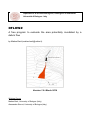
1
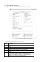
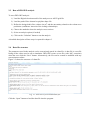
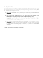
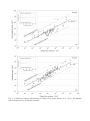
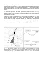
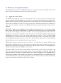
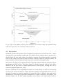
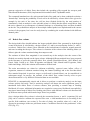
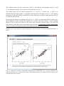
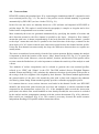
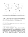
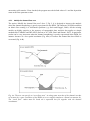
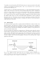
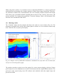
Dipartimento di Scienze Biologiche, Geologiche e Ambientali Università di Bologna - Italy DFLOWZ A free program to evaluate the area potentially inundated by a debris flow by Matteo Berti ([email protected]) Version 1.0- March 2014 Working Group Matteo Berti, University of Bologna (Italy) Alessandro Simoni, University of Bologna (Italy) Table of contents 1 Introduction ............................................................................................................................................... 3 2 Getting started .......................................................................................................................................... 5 2.1 Installing DFLOWZ.............................................................................................................................. 5 2.2 The Graphical User Interface ............................................................................................................. 6 2.3 Run a DFLOWZ analysis ..................................................................................................................... 7 2.4 Data file structure .............................................................................................................................. 7 2.5 Sample data files ............................................................................................................................... 8 3 Theoretical background ............................................................................................................................. 9 4 Features and specifications ..................................................................................................................... 13 4.1 Digital Elevation Model ................................................................................................................... 13 4.2 Flow channel.................................................................................................................................... 14 4.3 Debris flow volume .......................................................................................................................... 15 4.4 Cross-sections .................................................................................................................................. 17 4.5 Analysis options ............................................................................................................................... 18 4.5.1 Start deposition from a specified cross-section ...................................................................... 18 4.5.2 Modify the channel flow area ................................................................................................. 19 4.5.3 Modify the DEM....................................................................................................................... 20 4.6 Showing results................................................................................................................................ 21 5 Release history ........................................................................................................................................ 23 6 References ............................................................................................................................................... 24 To download DFLOWZ and the electronic version of this user’s manual, please go to www. bigea.unibo.it/it/ricerca/dflowz If you have questions about DFLOWZ or its use, please contact: Matteo Berti: [email protected] 1 Introduction DFLOWZ is a free application that provides a preliminary evaluation of the area potentially inundated by a debris flow. The method is based on the empirical-statistical model originally proposed by Iverson et al. (1998) to predict the runout length and the areas affected by lahars (LAHARZ model). DFLOWZ extends the Iverson’s model to debris flow phenomena, taking into account of the unconfined flow that occurs on a depositional fan. Beside a digital elevation model (DEM), DFLOWZ has few input requirements: debris flow volume and possible flow-path. The procedure is implemented in Matlab and a Graphical User Interface helps to visualize initial conditions, flow propagation and final results. Different hypothesis about the depositional behaviour of an event can be tested together with the possible effect of simple remedial measures. Uncertainties associated to input parameters can be treated and their impact on results evaluated. DFLOWZ is intended for students and practitioners who need a simple method for debris flow susceptibility mapping. The method can be an alternative to more comprehensive numerical models when calibration data are not available, or when a preliminary hazard analysis is required. However, it is essential to be aware that DFLOWZ is a simple geometrical model that does not reproduce the complex dynamics of debris flow-channel interaction. Therefore, DFLOWZ cannot replace the existing numerical models that describe the physics of the phenomenon. This user manual describes how to use DFLOWZ and the key features of the program. Please refer to the reference papers listed below for details on the theory behind DFLOWZ as well as for the discussion of important issues such as choice of input parameters, interpretation of the results, and limitations of the method. Reference papers Berti M., Simoni A. (2014). DFLOWZ: a free program to evaluate the area potentially inundated by a debris flow. Computers & Geosciences, 67, 14-23. Simoni, A., Mammoliti, M., Berti, M. (2011). Uncertainty of debris flow mobility relationships and its influence on the prediction of inundated areas. Geomorphology, 132, 249–259. doi:10.1016/j.geomorph.2011.05.013. Berti, M., Simoni, A. (2007). Prediction of debris flow inundation areas using empirical mobility relationships. Geomorphology, 90, 144-161. doi:10.1016/j.geomorph.2007.01.014. Disclaimer DFLOWZ was developed for scientific purpose and it is free for non-commercial users. You are the sole responsible for your use of the program. The author and the University of Bologna are not responsible for any damage however caused which results, directly or indirectly, from your use of DFLOWZ. Acknowledgments This work was supported by the Italian Ministry of University and Scientific Research (PRIN 20102011, Ref. 2010E89BPY_005, “Time-space prediction of high impact landslides under the changing precipitation regimes”). 2 Getting started 2.1 Installing DFLOWZ DFLOWZ was developed in Matlab and compiled as a standalone application. The application can run on any windows system without having Matlab or its auxiliary toolbox. If you do not have Matlab installed on your computer (release R2011b or higher), download the “Installation package with Matlab libraries” (398 MB) and save it on your computer in a separate folder. The installation package contains: the DFLOWZ executable four sample data files the shared Matlab libraries Run the self-extracting executable and follow the instructions displayed by the setup program. The program will extract the DFLOWZ executable and the sample data files on the installation folder, and it will run the Matlab Compiler Runtime (MCR) The MATLAB Compiler Runtime (MCR) is a standalone set of shared libraries that enables the execution of compiled MATLAB applications or components on computers that do not have MATLAB installed. Once the installation is completed, you can run the DFLOWZ executable. If you have Matlab installed on your computer (release R2011b or higher with the Statistics Toolbox), just download the zip file (2.4 kB) that contains the DFLOWZ executable and the sample data files. Unzip the file and run the application. 2.2 The Graphical User Interface The Graphical User Interface (GUI) of DFLOWZ is shown in Fig. 2.1. Fig. 2.1. The DFLOWZ graphical user interface A short description of the GUI boxes is given below: Box 1 2 3 4 5 Description Load the Digital Elevation Model of the area (in ASCII grid format) Load the path of the flow channel (in shp format) Define the design volume of the debris flow and uncertainty parameters of the volume-area scaling relationships Define the method used to draw the analysis cross-sections (see below) Analysis options used to: (1) start the inundated area from a specified cross-section; (2) modify the channel geometry to account for excavated or filled areas , (3) modify the DEM to simulate levees, structures, or retention basins. 2.3 Run a DFLOWZ analysis To run a DFLOWZ analysis: 1) Load the Digital elevation model of the study area as ASCII grid file 2) Load the path of flow channel as polyline shape file 3) Define the design debris flow volume (in m3) and the uncertainty related to the volume-area prediction (confidence intervals of the scaling relationships) 4) Choose the method to draw the analysis cross-sections 5) Select an analysis option (if needed) 6) Click on the “Calculate” button to run the analysis A detailed description of these steps is reported in chapter 3. 2.4 Data file structure The parameters used in the analysis can be conveniently stored in a data file. A data file is a text file listing all the values used to run a simulation. DFLOWZ creates a text file (with “dfz” extension) when the user click the “Save” button. Alternatively, the file can be created or modified with any convenient text editor. Figure 2.2 shows the structure of a data file. Fig. 2.2. Structure of a DFLOWZ data file Click the “Open” button to load the data file into the program. 2.5 Sample data files Four sample data files are provided in the folder named “Sample”. The files share the same digital elevation model (dem.asc), flow channel path (channel.shp), and design debris flow volume (30000 m3), but differ in other analysis parameters: Case_01.dfz is the data file used to generate Fig. 4.6 (which is Fig. 9 in Berti and Simoni, 2014) Case_02.dfz uses the variables from case 1, but higher values of the confidence levels related to the two uncertainty parameters a and b (see Berti and Simoni, 2014) Case_03.dfz uses the “Modify the flow channel area” option (box 5 in Fig. 2.1) to simulate an excavation of 30 m2 in the upper reach of the flow channel; the values of the extra-flow area are listed in the text file “channel_mod.txt” Case_03.dfz uses the“Modify the DEM” option (box 5 in Fig. 2.1) to simulate the presence of a levee on the left side of the flow channel; the shapefile “levee.shp” contains the polygon to modify and the corresponding change in elevation (5 m) stored in the attribute field “ChangeEl” Click the “Open” button to load a sample file for testing. 3 Theoretical background A detailed description of the theory behind DFLOWZ can be found in Berti and Simoni (2007). In this section we briefly outline the general principles of the model. DFLOWZ extends to debris flows an empirical-statistical model originally proposed by Iverson et al. (1998) to predict the runout length and the areas affected by lahars (LAHARZ model). Both models are based on the simple observation that the larger the volume of the flow ( V ), the larger the cross-sectional flow area ( A ) and the inundate planimetric area ( B ). The dependence V A and V B has been documented for different types of flow (rock avalanches, lahars, debris flows) and reported in form of two semi-empirical scaling relationships (Griswold and Iverson, 2008; Scheidl and Rickenmann, 2010): A k AV 2 / 3 [1a] B k BV 2 / 3 [1b] where k A and k B are dimensionless coefficients (called mobility coefficients) that vary with the flow type and 2/3 is a fixed exponent justified by geometric similarity (Iverson et al., 1998). Simoni et al. (2011) combined the data of about 100 historical debris flows obtaining k A 0.07 and k B 18 (Fig. 3.1). These values can be considered of general validity for non-volcanic debris flows since no systematic difference was found between datasets collected in different geological environments. In reality, the mobility of debris flows is certainly influenced by water content, grainsize distribution, or debris availability, but these differences are masked by the scatter of the data due to measurement uncertainties. To account for the data dispersion around the regression lines, Simoni et al. (2011) proposed to include two “uncertainty factors” ( a and b ) in the scaling relations: A a 0.07V 2 / 3 [2a] B b 18V 2 / 3 [2b] The parameters a and b indicate how the expected values of A and B differ from that predicted by the regression lines shown in Fig. 3.1. The numerical values of a and b are plotted in the small insets of Fig. 3.1 as a function of the confidence level of the prediction, which measures the distance from the regression based upon the sample standard deviation and t-statistic (Weisberg, 1985). Fig. 3.1. Empirical scaling relationships for debris flows (from Simoni et al., 2011). The dashed lines indicate the 95% prediction intervals. Depending on the specific application, the uncertainty factors a and b allow the user to obtain predictions of the best/worst scenarios in terms of inundated and cross-sectional areas as a function of the appropriate confidence level. Also, different combinations of a and b allow to reproduce different expected debris flow velocity and mobility whenever information on the flow behavior is available. For instance, one might expect that a dilute flow inundates a small cross-sectional area ( a <1) because of its velocity, and deposits over a large planimetric ( b >1) area because of its mobility. Anyhow, the rationale of such observations is rarely solid enough to base any prediction on, and the statistic approach is preferable. Equations [2a] and [2b] are implemented in DFLOWZ to predict the inundated area on a debris flow fan. Input data are the debris flow volume V , the uncertainty factors a and b , the Digital Elevation Model (DEM) of the fan area, the path of the flow channel, and the traces of several representative cross-sections. For a given volume, the model first computes the expected value of cross-sectional ( A ) and planimetric ( B ) inundated area using equations [2a] and [2b]. The flow area A is assumed to be constant for any location along the depositional reach and it is used to compute the inundated width along the profiles extracted by the DEM (Fig. 3.2). Fig. 3.2. The planimetric inundated area (a) is estimated by interpolating the cross-sectional inundation widths (b) computed on several cross-sectional channel profiles. The expected values of cross-sectional flow area A and planimetric inundated area B are given by the two scaling relationships shown in Fig. 3.1. The calculation starts with the first section upstream and proceeds downstream determining the inundation area between the sections. The inundated area is progressively summed until it equals the expected value of B given by [2b]. The main difference between DFLOWZ and LAHARZ (Iverson et al., 1998; Schilling, 1998) is that our model is designed to (roughly) simulate unconfined flow deposition. When the flow exceeds the available channel area it is assumed that the debris deposits over the ground surface with a constant thickness h . The thickness of unconfined flow is a function of debris flow volume and it is simply obtained by dividing V by the expected B ( h 0.06 V 1/ 3 ; Fig. 3.2). 4 Features and specifications The Graphical User Interface of DFLOWZ (Fig.2.1) is divided into five tasks which allow for the input of physical parameters and selection of run-time options. 4.1 Digital Elevation Model The DEM must include the active part of the fan, that is the area where relatively recent deposition, erosion, and alluvial-fan-flooding have occurred. This area typically contains the active debris flow channel, which is the most probable path for future events (Glade, 2005). When the identification of active zones is difficult, or when it is likely to have flow diversion from the active channel, the entire fan area should be included in the DEM and different potential debris flow paths must be analyzed. DFLOWZ is adapted to run with high resolution digital elevation models (1 to 3 m cell size) such as those derived from airborne LiDAR data. Care should be taken when using coarse resolution DEMs (10 m cell size or larger) since the flow channel can be poorly represented and this will have important consequences on simulation results. In general, a smoothed topography will produce an inundation area which is wider and shorter than expected because a low resolution DEM underestimates the available area of the flow channel and the debris flow will inundate a large width to accomplish the theoretical value of A (Fig. 4.1). The main risk in these cases is to underestimate the runout distance and to spread the flow too much sideways. DEMs often contain erroneous elevations referred to as “sinks” that are usually “filled” before hydrological modeling. However, some sinks may represent real surface depressions where the debris can be trapped then reducing the flooded area. The user must be aware of real topography to determine whether sinks in the DEM are errors or not. The largest DEM array that can be loaded mainly depends on the system memory (RAM plus swap file) and operating system. By assuming that no major processing are launched and that an unlimited memory is available, the largest matrix size is about 1500 MB for 32-bit platforms and 16 GB for 64-bit platforms. This roughly corresponds to a maximum DEM size of 14000x14000 cells or 46000x46000 cells respectively. Input data file is an ASCII Grid (6 lines of header info followed by the elevation data) compatible with most GIS software. Fig. 4.1. Effect of the DEM resolution of the inundated cross-sectional width. The inundated width tends to be larger for a low-resolution channel profile (b). 4.2 Flow channel DFLOWZ calculates the deposition area by assuming a constant cross-sectional flow area A which extends across a user-specified channel path. The path of the flow channel must be specified by a polyline shape file (one single feature, no attributes required). The channel path has a profound effect on the results because the flooded area always wanders around the predefined channel. A proper definition of the potential flow path is therefore essential for meaningful results. In most cases, it is quite easy to identify the active debris flow channel on the fan by means of aerial photographs and field surveys. The active channel is directly connected with the main feeder channel at the fan apex and it is usually characterized by fresh deposits, scouring, bare soil or scattered vegetation (Hungr et al., 2005). However, when there is no morphological evidence of recent activity, or there are no historical records of past events, the choice of a likely debris flow pathway can be difficult. In this case it is necessary to perform a sensitivity analysis to evaluate the effect of different flow paths on the inundated area. The method proposed by Hurlimann et al. (2008) is suitable to this purpose. The method combines the D8 flow routing algorithm with a Monte Carlo random walk model to generate trajectories of debris flows that include the spreading effect around the steepest path. Scheidl and Rickenmann (2010) implemented this method in their TopRunDF model. The computed inundated area for each potential debris flow path can be then combined to obtain a “hazard map” showing the probability of each cell to be affected by a future debris flow (given for example by the ratio of the times the cell has been flooded divided by the total number of simulations). Such an analysis is also advisable when it is likely that the debris would divert from the active channel (as a consequence of channel blockage or overbanking flow) and flow downhill on the fan. The probabilistic analysis of the multiple channel paths is not implemented in the current version of the program, but it can be easily done by combining the results obtained with different channel paths 4.3 Debris flow volume The design debris flow should indicate the largest probable debris flow generated by hydrological events in the basin. It is defined by a design volume ( V ) and by two uncertainty factors ( a and b , see above). Debris flow volume is here intended as the total amount of sediment, organic material, and water reaching the fan apex. This volume is a function of the volume of the initiating failure (or failures) plus the volume entrained along the transport reach. The estimate of debris flow magnitude is an essential step in the analysis since the extent of the flooded area mainly depends on the input volume. Although different methods have been proposed in the literature to guess the potential debris flow volume (Kronfellner-Kraus, 1985; Bianco and Franzi, 2000; Ceriani et al., 2000; D’Agostino and Marchi, 2001; Marchi and D’Agostino, 2004; Jakob and Hungr, 2005) this estimate still remains a difficult task. The main uncertainties are related to sediment availability, expected water inflow, effect of vegetation, amount of sediment entrained along the channel (bulking) and to the fact that debris flow material deposited in previous surges (or delivered by bank failure) can be remobilized in subsequent surges. In practice, the estimate of the debris flow volume heavily relies on past observations and it is very difficult if historical data are not available. DFLOWZ is computationally simple and it allows to perform a sensitivity analysis on the input volume quickly and easily. Such a sensitivity analysis will detect the most significant zones of inundation from debris flows of various volumes, thus providing a scenario map of flooding likelihood. Of course, additional information are required to convert any likelihood (susceptibility) map into a hazard map of debris flow flooding since flows with different volumes are characterized by different return periods which make larger flows less probable. Once a design debris flow volume is selected, the uncertainty factors a and b (equations [2a] and [2b]) can be varied to calibrate the expected flow area A and inundated area B according to the specific field conditions (see section 2). For sake of clarity, the possible values of a and b are reported as percentages in the two pull-down menus “Confidence interval for the predictions” of the GUI (Fig. 2.1). The confidence intervals can be varied from –90% to + 90% and the corresponding values of a and b are computed using the curves shown in the small insets in Fig. 3.1. The default values are 0% which correspond to a 1 and b 1 . In this case, A and B are estimated from the input volume V using the mean regression lines shown in Fig. 3.1. The implicit assumption is that the mobility of debris flows in the study area is similar to that typically observed for subaerial debris flows. By selecting for instance a confidence interval for b 90% we assume that the flow can be more mobile than the average, and that the inundated area will be larger than usually is. In the example shown in Fig. 4.2, the user selected a=0% and b=60%, then the expected values of A and B fall respectively on and above the corresponding regression lines. Click on the “Charts” button of the GUI to see where the design flow plots with respect the two scaling relationships. Simoni et al. (2011) provide several indications on the selection of the uncertainty parameters a and b . Fig. 4.2. Empirical scaling relationships implemented in DFLOWZ. The red point indicates the expected value of cross-sectional flow area A (left) and planimetric inundated area B (right) for the selected debris flow volume. 4.4 Cross-sections DFLOWZ evaluates the inundated area B by connecting the inundation width Wi computed at each cross-sectional profile (Fig. 3.2). The traces of the profiles can be defined manually or generated automatically by DFLOWZ (see box 4 in the GUI, Fig. 2.1). In the first case the traces are manually drawn on a GIS software and imported in DFLOWZ as polyline shape file. This option is useful when the topography is complex or irregular and a close control on the computational cross-sections is needed. More commonly the traces are generated automatically by specifying the number of sections and their direction (normal to the flow channel or parallel to the slope). “Normal to flow channel” means that each trace is drawn perpendicularly to the local direction of the flow channel; “parallel to the slope” means that each trace is parallel to the local direction of the slope, evaluated as the mean aspect of a 3x3 kernel centered at the intersection point between the channel and the profile. Unless the flow channel cuts transversally the slope, the differences between these two options are usually minor. The traces are numbered consecutively from the first section upstream. Before running the analysis is important to check the location of the traces (“Map” button on the GUI; Fig. 2.1) to ensure the correctness of the result. Moreover, since the number, location, and direction of the profiles affect to some extent the flooded area, it is also important to evaluate the sensitivity of the analysis to such a factor. Two methods of surface interpolation can be selected to generate the cross-sectional profiles, referred to as “IDW” and “Planar” in the GUI. The IDW method (Inverse Weighted Distance method; Watson and Philip, 1985) calculates the unknown elevation at each point of the profile as the average of the five neighbor cells weighted by their distance. The Planar method approximates the ground surface of the nine cells around the point with a plane and computes the unknown elevation by planar fitting. Planar method typically provides a smoother topographic profile. It is common that two cross sections intersect near bends in the channel. In this case DFLOWZ identifies the intersection point between the two lines and compares it with the inundated width computed for the downstream section (Fig. 4.3): if the inundated width exceeds the intersection point (that is the debris flow would inundate an area already flooded) the cross-section is excluded by the analysis and the computation continues with the section downstream (Fig. 4.3b); otherwise, both sections are considered (Fig. 4.3a). This control is necessary because the model assumes independent flooding of 2D profiles without interaction effects. Fig. 4.3. In case of intersecting cross-sections, DFLOWZ checks if the intersection occurs along the inundated width or not. In first case (b), the downstream section is omitted and the computation proceeds with the section further downstream. In the second case (a) both the sections are maintained. The sample file “Case_01.dfz” can be used to test the different options provided by DFLOWZ to draw cross-sections. Open the file, choose an option, and compare the inundated area in the different cases. The “Sample” folder contains a shapefile with the traces of 14 user-defined crosssections (sections.shp) that must be loaded when the “User-defined” option is selected. 4.5 Analysis options Several options are available in DFLOWZ to take control of the analysis and possibly improve the representativeness of the prediction. 4.5.1 Start deposition from a specified cross-section The option “Start deposition from section” (box 5, Fig. 2.1) allows the user to evaluate the sensitivity of the results on the starting point of the deposition. As said above, the deposition starts at the first upstream section which is usually located at the fan apex. In some cases, however, the flow channel is deeply incised in the upper part of the fan and the deposition may take place only from a point further downstream; or the flow channel can be partially filled along its path and the deposition may start upstream the fan apex. The starting point of deposition is an important input parameter that should be chosen on the basis of a detailed geomorphological survey of the flow channel on the fan area. This option allows to evaluate how the flooded area varies if some uncertainty still remains. If not checked, the program uses the default value of 1 and the deposition starts at the first upstream section. 4.5.2 Modify the channel flow area The option “Modify the channel flow area” (box 5, Fig. 2.1) is designed to improve the analysis when the channel morphology is poorly represented in the DEM. The influence of DEM resolution on debris flow routing is a well-known problem (e.g. Stolz and Huggel, 2008). All the existing models are highly sensitive to the accuracy of topographic data, and this also applies to simple methods like LAHARZ and DFLOWZ (Stevens et al., 2002; Berti and Simoni, 2007). In particular, results can be very inaccurate when the channel morphology is poorly represented in the DEM, for instance because of a low spatial resolution (Fig. 4.4a) or because the channel has been filled or excavated (Fig. 4.4b). Fig. 4.4. The user can specify an “extra flow area” AE along some stretches of the channel in order to account for a poor resolution of the DEM (a) or to roughly simulate a channel excavation (b). The “extra flow” values must be listed on a separated text file together with the channel coordinates. To partially overcome this problem, DFLOWZ allows the user to import an external text file which contains, for each channel reach between points i and i 1 , an “extra flow” area AE (in m2) not represented in the DEM (Fig. 4.4). A positive value of AE will reduce the theoretical value of A on the selected channel reach, while a negative value will increase it. In the first case the inundated width will be smaller, simulating the presence of a larger channel; in the second case the inundated width will be larger, simulating the presence of a smaller channel. It is important to realize that AE only affects the theoretical flow area A while B does not vary. Therefore, the planimetric inundated area will be narrower around the channel reaches with AE >0 but it will extend longer downstream in order to attain the theoretical value of B . This feature can be also used for a preliminary evaluation of debris flow countermeasures such as channel excavation or widening. The data file Case_03.dfz provides a sample application of this option. 4.5.3 Modify the DEM The “Modify the DEM” option allows to quickly modify the DEM and to evaluate its effect on the deposition patterns. The DEM can be modified to generate 3D structures such as buildings or houses, to improve the accuracy of the topography, or to simulate the construction of channel levees or deflection walls. DFLOWZ takes advantage of the Matlab’s capability to read geodata files in order to perform this analysis easily. The areas to modify can be digitized as a polygon layer on a GIS and saved as a shape file, with the required change in elevation stored in an attribute field named “ChangeEl” (number data format, values in meters). DFLOWZ loads the polygon shape file and changes the elevations of grid cells inside the polygon according to the specified value (Fig. 4.5). A positive value will increase the elevation, a negative value will lower the topography. The data file Case_04.dfz provides a sample application of this option. Fig. 4.5. The “Modify the DEM” option allows the user to simulate a positive (ChangeEl>0) or negative (ChangeEl<0) variation of the ground topography. DFLOWZ reads the areas to modify from a polygons shapefile where ChangeEl is an attribute field. When using these options it is essential to bear in mind that DFLOWZ is a simple geometrical model that does not reproduce the complex dynamics of debris flow-channel interaction. Therefore, any simulation of debris flow countermeasures has to be carefully evaluated, and the final design must always rely on detailed hydraulic modeling that account for flow velocity, shear stress, and pressure gradient. For instance, the possibility of structure damage, failure, and subsequent flow diversion is not considered in DFLOWZ. 4.6 Showing results The “Calculate” button runs the analysis and shows the results on a new window (Fig. 4.6). The planimetric inundated area and the flow channel path are drawn on a low-resolution contour map (max 100x100 cells ) to speed up the display. Fig. 4.6. Sample results of DFLOWZ. Planimetric inundated area (left) and cross-sectional flow area for two selected profiles (right). The window provides a quick view of the results. For a more accurate display, click the “Export grid” button to save the inundated area in ASCII Grid format with the original DEM resolution. The grid can be then opened using most GIS software and combined with other digital maps and georeferenced data. The box “Show cross-section traces” shows the profiles used in the analysis (as said above, the intersecting cross-sections could be excluded by the analysis) while the button “Edit Figure” allows users to customize the appearance of the map and to save it as image using the built-in editing functions of Matlab. Click on the listbox “View section” to see the inundated flow area in each cross-section. The crosssectional profile is shown on a separate chart with the flow area colored in red (Fig. 4.6). Interactive zoom and pan (available as built-in Matlab functions) allow to check whether the model provides realistic results. A careful check of each cross-section is recommended in order to detect unexpected results related to particular topographic conditions. 5 Release history Do not hesitate to contact the author ([email protected]) if you find any error and bug, or if you have comments or suggestions to improve DFLOWZ. We need your feedback! Release Date 1.0 March 2014 Description First release of DFLOWZ 6 References Berti, M., Simoni, A. (2007). Prediction of debris flow inundation areas using empirical mobility relationships. Geomorphology, 90, 144-161. doi:10.1016/j.geomorph.2007.01.014. Berti M., Simoni A. (2014). DFLOWZ: a free program to evaluate the area potentially inundated by a debris flow. Computers & Geosciences, 67, 14-23. Bianco G, Franzi L. (2000). Estimation of debris flow volumes from storm events. In Debris-flow Hazards Mitigation: Mechanics, Prediction, and Assessment, WieczorekGF, NaeserND (eds.), Balkema, Rotterdam, 441- 448. Ceriani M., Crosta G., Frattini P. e Quattrini S. (2000). Evaluation of hydrogeological hazard on alluvial fan. Proc. Int. Symp. INTERPRAEVENT 2000, Villach, Band, 2, 213-225. D'Agostino V, Marchi L. (2001). Debris flow magnitude in the Eastern Italian Alps: data collection and analysis. Physics and Chemistry of the Earth, Part C 26 (9), 657- 663. Hungr, O., Fell, R., Couture, R., Eberhardt, E. (2005). Landslide Risk Management. Proceedings of the International Conference on Landslide Risk Management, Vancouver, Canada, 31 May-3 June 2005, Taylor & Francis, 776 pp. Hurlimann, M., Rickenmann, D., Medina, V., Bateman, A. (2008). Evaluation of approaches to calculate debris-flow parameters for hazard assessment. Engineering Geology, 102, 152–163. Iverson, R.M., Schilling, S.P., Vallance, J.W. (1998). Objective delineation of lahar-inundation hazard zones. Geological Society of America Bulletin, 110, 972-984. Jakob, M., Hungr, O. (2005). Debris-flow hazards and related phenomena. Springer, Chichester, UK, 798 pp. Kronfellner-Kraus G. (1985). Quantitative estimation of torrent erosion. In: International Symposium on Erosion, Debris Flow and Disaster Prevention, Tsukuba (Japan), A.Takei (ed.), 107110. Marchi L, D'Agostino V. (2004). Estimation of debris-flow magnitude in the Eastern Italian Alps. Earth Surface Processes and Landforms, 29, 207-220. Scheidl, C., Rickenmann, D. (2010). Empirical relationships for debris flow mobility and deposition on fans. Earth Surface Processes and Landforms, 35, 157–173. Schilling, S.P. (1998). LAHARZ; GIS programs for automated mapping of lahar-inundation hazard zones. U.S. Geological Survey Open-File Report, 98–638, 80 pp. Simoni, A., Mammoliti, M., Berti, M. (2011). Uncertainty of debris flow mobility relationships and its influence on the prediction of inundated areas. Geomorphology, 132, 249–259. doi:10.1016/j.geomorph.2011.05.013. Stevens N.F., Manville V., Heron D.W. (2002). The sensitivity of a volcanic flow model to digital elevation model accuracy: experiments with digitised map contours and interferometric SAR at Ruapehu and Taranaki volcanoes, New Zealand. J. Volcanol. Geotherm. Res., 119,89–105. Stolz A., Huggel C. (2008). Debris flows in the Swiss National Park: the influence of different flow models and varying DEM grid size in modelling results. Landslides, 5, 311 – 319. Watson, D., Philip, G. (1985). A refinement of inverse distance weighted interpolation. GeoProcessing, 2, 315-327. Weisberg, S. (1985). Applied Linear Regression. John Wiley & Sons, New York. 344 pp.