Download ADAS308: Charge exchange spectroscopy

ADAS308: Charge exchange spectroscopy process effective coefficients: l-resolved
The program analyses column (line-of-sight integrated) emissivity observations of
charge exchange spectroscopy lines from hydrogenic impurities, occuring through
neutral beam / plasma interaction, in terms of emission measure. It predicts the
column intensities of spectral components of the charge exchange lines, the Doppler
broadened line shapes and effective emission coefficients for arbitrary lines in an lresolved picture.
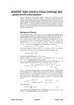
Background theory:
Charge exchange spectroscopy is driven by reactions of the form
+
0
X + z0 + Dbeam
(1) → X + z0 ( nl ) + Dbeam
4.8.1
in which an electron is captured from a donor atom in its ground (or an excited)
state. The principal application is usually to capture by the bare nuclei of impurity
atoms in the plasma from the ground state of deuterium, helium or lithium atoms in
fast neutral beams. Subsequently the hydrogen-like impurity ion radiates as
4.8.2
X + z0 −1 ( n ′l ′ ) → X + z0 −1 ( n ′′l ′′ ) + hν
Composite spectral line features of the form n′ → n ′′ are observed made up from
unresolved n′l ′ → n′′l ′′ multiplet components. Charge exchange line features often
involve high principal quantum shells and occur over wide spectral ranges including
the visible range. In general the populations of receiver levels are modified by
redistributive collisions with plasma ions and electrons and by fields before radiation
emission occurs. The present programme includes redistributive collisions of the
form
e
e
4.8.3
X + z0 −1 (nl ) +   → X + z0 −1 (nl ′) +  
Z µ 
Z µ 
where Zµ denotes a bare nucleus of charge Zµ and field induced redistribution of the
form
X + z0 −1 ( nl ) → X + z0 −1 ( nl ′ )
Bmag
[ not fully implemented] 4.8.4
The line-of-sight integrated photon emissivity of a charge exchange driven line may
be written as
z0 −1)
( z0 −1)
I n(→
n ′ = ∑ I nl → n ′l ′
l ,l ′
=
∫∑A
nl → n ′l ′
S l ,l ′
N nl( z0 −1) ds
= ∫ [ ∑ Anl →n ′l ′ ( N nl( z0 −1) / N D N ( z0 ) )] N D N ( z0 ) ds
S
l ,l ′
4.8.5
= ∫ [ ∑ q nl( eff→)n ′l ′ ] N D N ( z0 ) ds
S
l ,l ′
eff
z
= ∫ q n( →n)′ N D N ( 0 ) ds
S
)
( z0 )
ds
≈ q n( eff
→n′ ∫ N D N
S
where S is the path length through the neutral beam / plasma intersection along a
(z )
spectrometer line-of-sight. N D is the neutral donor number density and N 0 is the
( eff )
number density of fully ionised impurity atoms. qn → n ′ is the effective emission
ADAS User manual
Chap4-08
17 March 2003
coefficient for the whole n → n ′ principal quantum shell transition and
∫N
D
S
N ( z0 ) ds is the emission measure. The mean transition energy is
)
∆En,n′ = ( ∑ ∆E nl ,n′l ′ qnl( eff→)n′l ′ ) / qn( eff
→n′
4.8.6
l ,l ′
where ∆E nl ,n ′l ′ is the line component transition energy and qnl → n ′l ′ is the component
( eff )
( eff )
effective emission coefficient. The effective emission coefficient qn → n ′ may be
calculated theoretically. If it is approximately constant over the emitting volume,
( z −1)
then measurement of a charge exchange line intensity I n →0 n ′ allows deduction of the
emission measure
∫N
D
N ( z0 ) ds . If neutral beam attenuation to the observed
S
volume is known or calculable then local impurity density may be inferred.
Relationship to direct coefficients:
With the effective emission coefficients calculated theoretically, comparison with
one observed charge exchange line intensity allows deduction of the emission
measure. Then all other line intensities are predictable. If more than one line
intensity is observed, then a mean emission measure may be deduced and some
comment may be made on the ratios of exeperimental to theoretical effective
emission coefficients. The organisation of the collisional-radiative modelling in
ADAS308 is specifically designed to allow such comparison. The following points
and assumptions are made:
(i) From the theoretical point-of-view the direct capture cross-sections to levels are
more fundamental quantities for comparison with experiment that the effective
emission coefficients.
(ii) The dominant fundamental processes modifying the initial distribution of capture
are redistribution within an n-shell and radiative cascade in low and moderate density
plasmas. Limiting the collisional-radiative theory to these dominant processes allows
a compact invertable relationship to be established between column emissivities of
charge exchange spectrum lines and direct capture cross-sections.
(ii) It is of most practical value to target experiment / theory comparisons on the nshell distribution of capture (including the n-shell decrement) in fusion studies. This
may be achieved by imposing theoretical information on the l sub-shell distribution
of capture.
( CX )
Consider the monoenergetic direct capture rate coefficients to nl sub-levels qnl
from the initial neutral donor state D0(1) by the fully stripped impurity ion with
number density N
( z0 )
+
, denoted more compactly by N .
4.8.7
q ( Eu ) = v σ ( v )
where Eu is the relative collision energy per atomic mass unit so that
( CX )
nl
( CX )
nl
v = 2 Eu / mp is the relative collision speed, with mp the proton mass and σ the
capture cross-section.
It is supposed that
) ( CX )
qnl( CX ) ( Eu ) = f ((ntheor
q n ( Eu )
)l
4.8.8
Since no collisional excitation from lower to higher n-shells is allowed, the
populations of the lj sublevels of the principal quantum shell n′ ≥ n + 1 may be
written as
)
4.8.9
N n ′l ′ = N D N +
Wn′l ′ ,niv qn(CX
iv
∑
n iv ≥ n +1
Then the equations determining the populations of the sub-shells of the principal
quantum shell n are
) ( CX )
M (n)l ,l ′′ N nl ′′ = N D N + f (n(theor
qn +
Anl ,n′l ′ N n′l ′ 4.8.10
)l
∑
∑
n ′≥ n +1
l ′′
so that
ADAS User manual
Chap4-08
17 March 2003
N nlj = N D N +Wnlj ,n qn(CX ) + N D N +
∑
n iv ≥ n +1
with
)
Wnlj ,niv qn(CX
iv
4.8.11
)
( CX )
Wnlj ,n = [∑ M (−n1)lj ,l ′′j ′′ f ((ntheor
) l ′′j ′′ ]q n
4.8.12
l ′′j ′′
and
Wnlj ,niv =
∑M
l ′′, j ′′,l ′, j ′
−1
( n ) lj ,l ′′j ′′
Anl ′′j′′, n′l ′j ′Wn′l ′j ′,niv
4.8.13
The solution can proceed recursively downwards in n with compact vector and array
storage.
Tabulations of experimental or theoretical state selective charge exchange cross( CX )
section data span a range of principal quantum shells σ nlj ( v ) : n0 ≤ n ≤ n1 .
Cascade from levels n > n1 may contribute significantly to the populations of lower
levels especially at high collision energies when the decrease of the direct charge
−α
and α ~ 3). However,
exchange cross-sections with n is slow ( σ n ~ n
redistribution amongst lj sub-levels of the higher n-shells is high, approaching
statistical in most circumstances. Therefore the cascade solution is initiated at some
nmax (~20 typically) for complete n-shell populations only (matrices W (high) ), with
subshells implicitly statistically populated, down to n1 whereupon the lj resolved
( low )
solution (matrices W
) is commenced.
In general observable spectrum lines are associated with upper principal quantum
shells n ≤ n1 . If M rep , lines are identified each with a distinct upper n-shells
nirep : irep = 1,..., M rep , then a 'condensation' may be imposed such that
qn( CX ) =
M rep
∑L
irep=1
for n0 ≤ n ≤ n1
( CX )
n ,irep nirep
q
4.8.14
and
qn( CX ) = ( n / n1 ) α qn(1CX )
for n > n1
giving, after integration along the line-of-sight, a matrix relation
 I n →n
1
1′

.

I
 n M rep →n M′ rep
4.8.15

 a11 . . a1 M  q n( CX ) 
rep


 1 
+
.
.  . 
 = ( ∫ N D N ds)  .
)
S

a
. a M rep M rep  q n( CX

 M rep 1
  Mrep 
4.8.16
The coefficients of the matrix are theoretically calculated quantities. The equations
( CX )
may be solved for the the qn
i
and the emission measure
∫N
D
N + ds subject to
S
the constraint
M rep
∑q
irep=1
( CX )
nirep
=
M rep
∑q
irep=1
( CX )( theor )
nirep
4.8.17
Energy levels:
Precise energy levels are required in calculating collisional redistribution between the
degenerate and nearly degenerate states. This is also required in reconstructing
precise n-n' line feature shapes. The cases of hydrogen-like ions and lithium-like
ions are treated separately
Case(i): hydrogen-like ions
ADAS User manual
Chap4-08
17 March 2003
E (nl 2Ll +1/ 2 ) = − ( zeff2 1 / n 2 ) I H − RMC nl ( zeff 2 )
+ 21 l ZETAnl ( zeff 2 ) + δ l ,0QEDn ( zeff 2 )
2
2
E (nl 2Ll −1/ 2 ) = − ( zeff
1 / n ) I H − RMC nl ( zeff 2 )
4.8.18
+ 12 ( l + 1) ZETAnl ( zeff 2 )
where
(α 2 z 4 / n 4 )[(n / l + 21 ) − 43 ]I H l > 0
RMCnl ( z ) =  2 4 4
3
 (α z / n )[(n / l + 1) − 4 ]I H l = 0
(2α 2 z 4 / n 4 )[n / l (2l + 1)(l + 1)]I H l > 0
ZETAnl ( z ) = 
l=0
0
4.8.19
QEDn ( z ) = (8α z / 3πn ){ln[1 / ( α z ) ] +
3 4
3
2
19
30
+ Ln } I H
with L1=-2.984128, L2=4.811768, L3=-2.767699, L4=-2.749859 and Ln=2.71632-0.02402(5/n)3/2 . The effective charge prescription is zeff1 = zeff2 = z0.
Case (ii): lithium-like ions
E (1s 2 nl 2Ll +1/ 2 ) = E Edlen ( zeff 1 ) + 12 l ZETAnl ( zeff 2 )
E (1s 2 nl 2Ll −1/ 2 ) = E Edlen ( zeff 1 ) + 12 ( l + 1) ZETAnl ( zeff 2 ) 4.8.20
where the EEdlen are obtained from Ritz formulae for s and p orbitals and
from
polarisabilities for l > 1 due to Edlen (1979). The effective charge
prescription is zeff1 = z0, zeff2 = z0.-2.
Alternate driving processes:
Primary fundamental state selective charge exchange cross-section data for the
calculations are taken from ADAS compilations (type ADF01) in general. For
contrast, a calculation may be carried out using state selective cross-sections from
analytic expressions in the high energy Eikonal approximation. These analystic
expressions are available for 1s, 2sand 2p donor states of neutral hydrogen and for
the 1s2 and 1s2s states of neutral helium. It is of interest to compare the analysis
with that which would occur with two alternative driving mechanisms. These are
free electron capture and collisional excitation by electron impact from the ground
state of the hydrogen-like impurity ion. The previous formulation remains the same
but with the emission measure and capture rate coefficients redefined as
∫N
e
N + ds
and
qn(irec)
4.8.21
∫N
e
N ( z0 −1) (1s)ds
and
( exc )
q1→
ni
4.8.22
S
or
S
respectively.
Source data :
The program operates on collections of fundamental state selective charge exchange
cross-section data. The allowed content, organisation and formatting of these files
are specified in ADAS data format ADF01. Centrally supported data collections are
stored in directories such as
/.../adas/adas/adf01/qcx#h0/
where the h0 identifies neutral hydrogen is the donor. The individual data set names
take the form
qcx#h0_<code>.#<ion>.dat
where <code> is a three character identifier of the source and <ion> is the receiving
fully ionised ion (for example c6). More detail is given below.
ADAS User manual
Chap4-08
17 March 2003
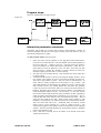
Program steps:
These are summarised in the figure below.
Figure 4.8
!
VHOHFW FKDUJH
H[FKDQJH GDWD
!
ILOH
ILOH HVWDEOLVK
QVKHOO UDQJHV
!
!
HQWHU XVHU
GDWD
SUHSDUH DOO
DWRPLF GDWD LQ
ORRNXS WDEOHV
DQG IUDFWLRQV
UHSHDW
!
!
UHSHDW
UHDG DQG YHULI\
EHJLQ
2XWSXW WDEOHV
DQG JUDSKV
SUHSDUH
HQG
WDEXODWLRQV
RXWSXW
GLVSOD\ VHOHFWHG
FROXPQ
HPLVVLYLWLHV
FRPSXWHVROQ
DFFRGLQJ WR
HPLVVLRQ
PHDVXUH W\SH
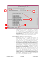
Interactive parameter comments:
ADAS308, which make use of data from archived ADAS datasets, initiates an
interactive dialogue with the user in three parts, namely, input file selection, entry of
user data and disposition of output.
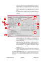
The file selection window is shown below.
1.
2.
3.
4.
ADAS User manual
Data root shows the full pathway to the appropriate data subdirectories.
Click the Central Data button to insert the default central ADAS pathway to
the correct data type – ADF01 in this case. Note that each type of data is
stored according to its ADAS data format (adf number). Click the User
Data button to insert the pathway to your own data. Note that your data
must be held in a similar file structure to central ADAS, but with your
identifier replacing the first adas, to use this facility.
The Data root can be edited directly. Click the Edit Path Name button first
to permit editing.
Available sub-directories are shown in the large file display window. Scroll
bars appear if the number of entries exceed the file display window size.
There are a large number of these. They are stored in sub-directories by
donor which is usually neutral but not necessarily so (eg. qcx#h0). The
individual members are identified by the subdirectory name, a code and then
fully ionised receiver (eg. qcx#h0_old#c6.dat). The data sets generally
contain nl-resolved cross-section data but n-resolved and nlm-resolved are
handled. Resolution levels must not be mixed in datasets. The ADF01 file
nmaes distinguish different sources. The first letter o or the code old has
been used to indicate that the data has been produced from JET compilations
which originally had parametrised l-distribution of cross-sections. The nlresolved data with such code has been reconstituted from them. Data of
code old is the preferred JET data. Other sources codes include ory (old
Ryufuku), ool (old Olson), ofr (old Fritsch) and omo (old molecular orbital).
There are newer data such as kvi. Additional codes are used for excited
donors such as ex2 for hydrogen n=2. Click on a name to select it. The
selected name appears in the smaller selection window above the file display
window. Then the individual datafiles are presented for selection. Datafiles
all have the termination .dat.
Once a data file is selected, the set of buttons at the bottom of the main
window become active.
Chap4-08
17 March 2003
1
2
3
4
5
6
.5
6.
7.
Clicking on the Browse Comments button displays any information
stored with the selected datafile. It is important to use this facility to
find out what has gone into the dataset and the attribution of the dataset.
The possibility of browsing the comments appears in the subsequent
main window also.
Clicking the Done button moves you forward to the next window.
Clicking the Cancel button takes you back to the previous window
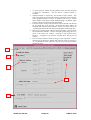
The processing options window has the appearance shown below
1.
2.
3.
4.
ADAS User manual
An arbitrary title may be given for the case being processed. For
information the full pathway to the dataset being analysed is also
shown. The button Browse Comments again allows display of the
information field section at the foot of the selected dataset, if it exists.
Information is given on the fully ionised impurity receiver and the
neutral beam donor. The atomic mass of the receiver must be entered.
The specification of beam parameters, details of observed line of sight
spectral emissivities to be analysed and emissivities to be predicted are
required. Input data of each of these three types may be addressed in
turn by activation of the relevant button. The window below the button
list then presents the appropriate table.
The Required emissivity predictions button is displayed. This activates
the predictive part of the code which becomes possible once the
observed lines have been analysed in terms of emission measure. Then
any set of lines within the N-shell limits may be predicted. The
standard output includes the mean wavelength and effective emisison
coefficient, but for up to five lines an extended tabulation of line
component emissivities may be produced. Graphs may be produced for
two selected line. Indicate these selections in the Key columnThe table
may be edited by clicking on the Edit Table button.
Chap4-08
17 March 2003
5.
6.
The Observed spectrum lines table allows introduction of a number of
observed intensities. It is possible to enter values which do not allow a
consistent solution. The code advises of this but it is the responsibility
of the user to check that the data is unblended etc. It is also a usual
practice to enter just one line, possibly with a fictitious emissivity
merely to obtain effective emission coefficients and line component
details.
The Beam parameter information button causes display of the third
editable table in the sub-window. Note that no check is made that the
various beam energy fractions sum to unity. This is the responsibility
of the user.
2
1
5
3
7
6
8
4
9
10
7.
Enter the plasma environment parameters. These determine the
collisional redistribution of the populations of the recombined plasma
ion. For ADAS308, B Magn. has no effect, but a value should be
entered as a place holder.
8. The final sub-window allows model and theory choices. Details are
given in the ADAS Manual. For each type, clicking on the selection
window drops down a short menu of choices. Click on the appropriate
choice. The ADAS data base source numerical data of type ADF01 is
the most usual, that is the Use input data set choice button. Note that
the Select emission measure model choice includes Electron impact
excitation as well as Charge exchange.
9. Extended information on the rates used in the populaiton modelling
may be printed.
10. Clicking the Done button causes the next output options window to be
displayed. Remember that Cancel takes you back to the previous
window.
The Output options window is shown below. Note that two plots are produced if
required. The Plot A is the stick diagram of component line-of-sight emissivities.
The Plot B is of the Doppler broadened profile of the line at the plasma ion
temperature.
ADAS User manual
Chap4-08
17 March 2003
1.
2.
3.
4.
5.
As in the previous window, the full pathway to the file being analysed
is shown for information. Also the Browse comments button is
available.
Graphical display is activated by the Graphical Output button. This
will cause a graph to be displayed following completion of this window.
When graphical display is active, an arbitrary title may be entered
which appears on the top line of the displayed graph. By default, graph
scaling is adjusted to match the required outputs.
Press the Explicit Scaling button to allow explicit minima and maxima
for the graph axes to be inserted. Activating this button makes the
minimum and maximum boxes editable. Plot A axes limits refer to the
‘stick diagram and Plot B axes limits to the Doppler broadened profile.
Hard copy is activated by the Enable Hard Copy button. The File name
box then becomes editable A choice of output graph plotting devices is
given in the Device list window. Clicking on the required device
selects it. It appears in the selection window above the Device list
window.
The Text Output button activates writing to a text output file. The file
name may be entered in the editable File name box when Text Output is
on. The default file name ‘paper.txt’ may be set by pressing the button
Default file name.
1
2
3
4
5
ADAS User manual
Chap4-08
17 March 2003
The Graphical output window is shown below
1. Printing of the currently displayed graph is activated by the Print button.
1
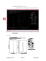
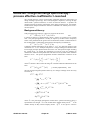
Illustration:
.
Figure 4.8a
ADAS User manual
Chap4-08
17 March 2003
The analysis of charge exchange emission by the code is shown in figure 4.8a and
+5
table 4.8a. Emission following electron capture by B from neutral deuterium
beam atoms in their ground state is illustrated. A single observed line-of sight
emissivity in the transition BV (n = 6 ---> n = 5) is analysed. Figure 4.8a shows the
theoretical breakdown of emission in the above line into multiplets and the expected
Doppler broadened profile of the feature
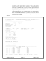
Table 4.8a shows the tabular output. A detailed tabulation of the component photon
fluxes is allowed for three spectrum line. In this case BV (n=6-5) is the ‘observed
line’. For the other selected charge exchange lines the predicted photon fluxes are
computed using the calculated emission measure. The spectrum lines BV (n=5-4)
and BV (n=4-3) are so tabulated.
Table 4.8a
ADAS RELEASE: ADAS93 V1.13 PROGRAM: ADAS308 V1.6 DATE: 16/04/98 TIME: 13:10
****** TABULAR INPUT FROM
L-RESOLVED CHARGE EXCHANGE EMMISIVITY PROGRAM: ADAS308-DATE:16/04/98 *****
------------------FILE: /home/anderson/adas/adf01/qcx#h0/qcx#h0_old#b5.dat
ELEMENT SYMBOL
NUCLEAR CHARGE
RECOMBINING ION CHARGE
RECOMBINED ION CHARGE
ATOMIC MASS NUMBER
=
=
=
=
=
RECEIVER
-------B
5
5
4
14.00
-------------------
NEUTRAL DONOR
------------H
1
-
PLASMA PARAMETERS:
ION TEMPERATURE
ION DENSITY
PLASMA EFFECTIVE Z
(EV)
=
(CM-3) =
=
BEAM PARAMETERS:
NUMBER OF BEAM COMPONENTS =
INDEX
5.00D+03
2.50D+13
2.00
ELECTRON TEMPERATURE (EV)
=
ELECTRON DENSITY
(CM-3) =
MAGNETIC INDUCTION
(T)
=
5.00D+03
5.00D+13
3.00
3
FRACTION
ENERGY
(EV)
------------------------------1
0.830
8.00D+04
2
0.100
4.00D+04
3
0.070
2.70D+04
OBSERVED SPECTRUM LINES:
NUMBER OF OBSERVED SPECTRUM LINES =
INDEX
NU
1
NL
COL. EMIS.
(PH CM-2 SEC-1)
--------------------------------1
6
5
1.00D+12
CHARGE EXCHANGE MODEL : INPUT DATA SET
EMISSION MEASURE MODEL: CHARGE EXCHANGE
EMISSION MEASURE (CM-5) =
5.1394D+19
N
QEX(N)
QTHEOR(N)
(CM3 SEC-1)
(CM3 SEC-1)
-------------------------------6
3.7316D-08
3.7316D-08
---------------------------------------- PREDICTED EMISSIVITES ----------------------------------N L
N1 L1
COL. POP.
COL. EMIS.
AIR WVLN.
(CM-2)
(PH CM-2 SEC-1)
(A)
-----------------------------------------------------------------------6 0
5 1
1.0898D+01
1.8275D+09
2981.51
6 1
5 2
2.3622D+01
1.4171D+09
2981.75
6 1
5 0
2.3622D+01
3.5889D+09
2980.26
6 2
5 3
9.3747D+01
2.2909D+09
2981.64
6 2
5 1
9.3747D+01
2.6350D+10
2980.65
6 3
5 4
2.3080D+02
1.6414D+09
2981.63
6 3
5 2
2.3080D+02
1.0438D+11
2981.17
6 4
5 3
4.1148D+02
2.8450D+11
2981.37
6 5
5 4
5.5806D+02
5.7400D+11
2981.48
-----------------------------------------------------------------------SUMS =
1.3286D+03
1.0000D+12
MEAN WVL(A) =
2981.39
EFF. RATE COEFFT. = 1.9457D-08
ADAS User manual
Chap4-08
17 March 2003
(CM-2)
(PH CM-2 SEC-1)
(A)
-----------------------------------------------------------------------5 0
4 1
1.7194D+01
6.9357D+09
1619.35
N 1
L
N1
L1
COL. POP.
COL. EMIS.
AIR
WVLN.
5
4 2
1.7510D+01
2.0636D+09
1619.52
5 1
4 0
1.7510D+01
8.0720D+09
1618.66
5 2
4 3
9.6686D+01
3.0518D+09
1619.48
5 2
4 1
9.6686D+01
8.9831D+10
1618.91
5 3
4 2
3.0982D+02
5.0070D+11
1619.22
5 4
4 3
6.7088D+02
1.7847D+12
1619.35
-----------------------------------------------------------------------SUMS =
1.1121D+03
2.3953D+12
MEAN WVL(A) =
1619.30
EFF. RATE COEFFT. =
N
L
N1
COL. POP.
COL. EMIS.
AIR WVLN.
(CM-2)
(PH CM-2 SEC-1)
(A)
-----------------------------------------------------------------------4 0
3 1
4.5713D+01
5.2466D+10
761.66
4 1
3 2
1.8361D+01
3.9904D+09
762.10
4 1
3 0
1.8361D+01
3.5193D+10
760.40
4 2
3 1
1.2747D+02
5.6097D+11
760.94
4 3
3 2
5.1345D+02
4.4270D+12
761.59
-----------------------------------------------------------------------SUMS =
7.0500D+02
5.0796D+12
MEAN WVL(A) =
761.51
EFF. RATE COEFFT. =
SUMMARY OF EMISSIVITIES:
N
N1
COL. POP.
COL. EMIS.
AIR WVLN.
EFF. COEFFT.
(CM-2)
(PH CM-2 SEC-1)
(A)
(CM3 SEC-1)
------------------------------------------------------------------------6
5
1.3286D+03
1.0000D+12
2981.39
1.9457D-08
5
4
1.1121D+03
2.3953D+12
1619.30
4.6607D-08
4
3
7.0500D+02
5.0796D+12
761.51
9.8836D-08
4.6607D-08
L1
9.8836D-08
Notes:
ADAS User manual
Chap4-08
17 March 2003