Download Bulletin for ADAS v1.7

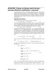
jul18-96
ADAS Bulletin
Five new programs are ready. The ADAS series 2 collisional radiative code, ADAS206, is now
operational. This code is very similar to the basic excited populaton code ADAS205 but is focused on
radiated power. Two more ADAS series 3 collisional radiative processing codes for charge exchange
spectroscopy are operational. These are ADAS306 and ADAS307. They are functionally very similar
to ADAS308 and ADAS309. That is they allow investigation of charge exchange spectroscopy line
intensities and predict effective emission coefficients for such lines respectively. However ADAS306
and ADAS307 are a little more advanced in that they work in J resolution. Finally ADAS406 from
ADAS series 4 is released. This code is analagous to the code ADAS405 for calculating metastable
resolved equilibrium ionisation balance and related photon emission functions. However ADAS406
evaluates the transient ionisation state of a plasma evolving in time in a simple model. It also evaluates
photon excesses or deficits compared with equilibrium emission. Thus ADAS406 complements
ADAS405 by allowing investigation of dynamic ionisation.
1.
ADAS206
This is a basic excited population structure modelling code with similar functionality to
ADAS205. Thus itt computes excited populations of an ion in a plasma and relates them to
designated metastable populations of the ion. ADAS206 differs from ADAS405 in that it
calculates also the total radiated power by the ion and the power emitted in one selected
spectrum line. Also, output datasets of these powers can be produced which follow the format
specification adf11. Calculations are performed at arbitrary temperatures and densities. Free
electron recombination and charge exchange recombination are handled, provided such data
is in the accessed datafile for the ion. The coupling to the continuum of the ion is however
simplified. In these respects ADAS206 and ADAS205 are identical. The advanced population
code ADAS208 treats these issues in a more sophisticated manner.
1.1.
1.2.
Initiate ADAS, move to the series 2 menu and click on the fifth button to activate
ADAS206.
The file selection window has the appearance shown below
1.2.1. Data root a) shows the full pathway to the appropriate data subdirectories.
Click the Central Data button to insert the default central ADAS pathway to
the correct data type. The appropriate ADAS data format for input to this
program is adf04 (‘specific ion files’). Click the User Data button to insert
the pathway to your own data. Note that your data must be held in a similar
file structure to central ADAS, but with your identifier replacing the first
adas, to use this facility.
1.2.2. The Data root can be edited directly. Click the Edit Path Name button first
to permit editing.
1.2.3. Available sub-directories are shown in the large file display window b).
Scroll bars appear if the number of entries exceed the file display window
size.
1.2.4. Click on a name to select it. The selected name appears in the smaller
selection window c) above the file display window. Then its sub-directories
in turn are displayed in the file display window. Ultimately the individual
datafiles are presented for selection. Datafiles all have the termination .dat.
1.2.5. Once a data file is selected, the set of buttons at the bottom of the main
window become active.
1.2.6. Clicking on the Browse Comments button displays any information stored
with the selected datafile. It is important to use this facility to find out what
is broadly available in the dataset. The possibility of browsing the comments
appears in the subsequent main window also.
1.2.7. Clicking the Done button moves you forward to the next window. Clicking
the Cancel button takes you back to the previous window
ADAS206 INPUT
Input COPASE Dataset
Data root /disk2/adas/adas/adf04/
Central data
Edit Path Name
User data
a)
belike/belike_jl1990c.dat
EHOLNHBMOFGDW
EHOLNHBMORGDW
c)
b)
'DWD )LOH
Browse Comments
1.3.
Cancel
Done
The processing options window has the appearance shown below.
1.3.1. At the top of the window, an appropriate Title for Run may be entered. Note
that name of the adf04 file selected for analysis is given immediately below
this. Also the Browse Comments button is present allowing scrutiny again of
the comments section of the adf04 file.
1.3.2. Plasma temperatures and densities for the population calculation are
required. The information on these and the facility for entering temperature
and density data are given in the sub-window at b). Click on the appropriate
button at a) to display the temperature or density information.
1.3.3. In both cases the further operations are the same. For the Densities subwindow, click on the Edit Table button to open up the table editor. The data
entry techniques and operations of Table Editor have been described
previously. Note that altering units (which must be done with the Table
Editor window activated) interprets the entered values in the selected units.
It does not convert values already typed in. Default densities may be
entered by clicking the appropriate button. The default values are inserted in
reduced units for ADAS206. Note that the ion density, neutral hydrogen
density to electron density ratio, NH/Ne and z+1 (≡z1) ionisation stage
density to z ionisation stage density, N(z1)/N(z), are only used if such
collisional data is present in the input adf04 file. The ion density and ratio
vectors are specified at each electron density so they must be of the same
length as the electron density vector. That is a model is specified.
1.3.4. TheTemperatures table is handled in like manner. Note that unlike the
density case, there is a set of input electron temperatures from the selected
adf04 file. The output electron temperatures are independent of the electron
densities so that final calculated populations are obtained at points of a twodimensional temperature/ density grid.
1.3.5. The Metastable State Selections button c) pops up a window indexing all the
energy levels. Activate the buttons opposite levels which you wish treated as
metastables. See the ADAS User Manual for a detailed explanation of the
handling of metastables in the collisional-radiative picture.
1.3.6. The basic power calculation uses the populations of the set of levels present
in the adf04 file. Some improvement may be made by extrapolating to
higher levels. Chose at d) a level above which an extrapolation correction is
to be added in. This means that each contributions to the power from a level
above the designated one will be enhanced by a correction. Noe extrpolation
is an option.
In the output paper.txt file, a tabulation of power coefficient ratios is given.
The ratio may be formed by using the power coefficient at zero density as the
denominator or the power coefficient at the lowest entered density. Make the
appropriate choice at e). Also at e) choose whether the power coefficient is
to be normalised to the ground state population to the whole stage
population. This option is only available when a single metastable (namely
the ground state) is selected at c).
1.3.7.
ADAS206 PROCESSING OPTIONS
Title for Run
demonstration
a)
Select temperatures and densities
for display:
Temperatures
Data File Name : /disk2/adas/adas/adf04/belike/belike_jl1990c.dat
Browse comments
Nuclear Charge : 24
Ion Charge : 0
Densities
d)
c)
b)
Metastable States
2s2(1S)
2s2p(3P)
(1)S( 0.0)
(3)P( 4.0)
Densities
6HOHFW H[WUDSRODWLRQ IRU
SRZHU
NO EXTRAPOLATION
NO EXTRAPOLATION
2s2(1S)
(1)S( 0.0)
2s2p(3P)
(3)P( 4.0)
Index
Electron
Densities
Ion
Densities
1
2
3
4
5
1.000E-03
0.0
...
...
...
...
NH/NE
Ratio
0.0
N(Z1)/N(Z)
Ratio
0.0
Selections
Density Units :Reduced
Selection
Selection
Line power ratios : density type for denominator
ZERO
Single metastable : normalise line power to the
total stage population
YES
Edit Table
Default Densities
e)
Select Electron Impact Transition of Specific Line
TRANSITION
------ LOWER LEVEL -----Selection
INDEX
INDEX DESIGNATION
Reaction Selection
------UPPER LEVEL -----INDEX DESIGNATION
Proton Impact Collisions
Scale Proton Impact for Zeff
1
1
Selection
1
1
1
1
2s2(1S)
(1)S( 0.0)
2 2s2p(3P)
(3)P( 4.0)
2s2(1S)
2s2(1S)
(1)S( 0.0)
(1)S( 0.0)
2 2s2p(3P)
3 2s2p(1P)
(3)P( 4.0)
(1)P( 1.0)
Enter Z-effective for Collisions
Ionisation Rates
Neutral H Charge Exchange
Free Electron Recombination
g)
Cancel
Done
f)
1.3.8.
The power coefficient for a particular radiative transition may be selected.
Click on the required transition at f). A file of format adf11 will be available
for output for this specific line power if requested.
1.3.9. Various processes, supplementary to the primary electron excitation
collisions and bound-bound radiative transitions, are activated as desired by
clicking on the appropriate buttons g). As for ADAS205, these only have an
effect if such data is present in the adf04 file, with the exception of
Ionisation Rates. This activates ionisation out of excited states and is
obtained by an internal calculation of these rates in the Burgess-Chidichimo
approximation. Warning-ionisation should not be switched on if you have
included autoionising levels in your adf04 dataset.
1.3.10. Proton collisions may be present in the adf04 file. If so, these rate
coefficients may be scaled to represent a mixture of other charged projectiles
with a mean Z-effective e).
1.4.
The output options window has the appearance shown below. It follows the familiar
form but with the added option of creating two output files.
1.4.1.
1.4.2.
Click on the button Graphics to obtain the sub-window for graphical output
settings. Click the button Text to obtain the sub-window for text and other
file output. This is also shown below.
In the first case, the button Graphical Output a) is activated to obtain display
of graphs. Select the temperature at which you wish populations graphed at
b).
ADAS206 OUTPUT OPTIONS
Data file name : /disk2/adas/adas/adf04/belike/belike_jl1990c.dat
Browse comments
Select output option settings for display
Graphics
Graph Temperature
Graphical Output
Graph Title
Text
2.00E+01
demonstration
a)
Explicit Scaling
X-min :
X-max :
Y-min :
Y-max :
5.00E+00
7.00E+00
1.00E+01
2.00E+01
b)
Select Device
Enable Hard Copy
File name : graph.ps
Cancel
1.4.3.
1.4.4.
1.4.5.
1.4.6.
1.4.7.
Replace
Post-script
Post-script
HP-PCL
HP-GL
Done
Default graph scaling may be over-ridden. Click the button for Explicit
Scaling and enter the required x and y axes limits.
To allow printing of hard copy of graphs, click the button Enable Hard Copy.
Note the selection of graphic output device is made at c). The Select Device
is chosen by clicking on a device in the lower window and the selection is
displayed in the upper window.
In the Text sub-window, the Text Output file may be selected as usual.
The Contour File button d) should be activated to write the passing file for
use by the diagnostic line ratio program ADAS207. This is as for ADAS205.
There is no arrangement for permanent storage of such files which reside
only in a user’s file space and are generally prepared for temporary
immediate use. Usually in ADAS we store such temporary ‘passed files’ in a
pass sub-library. You should create this at the first level within the adas
database as
/...../<uid>/adas/pass
By default ADAS206 sends the contour file to
/...../<uid>/adas/pass/contour.pass
The Total Line Power File button e) and the Specific Line Power File button
f) should be activated to write the appropriate passing files. They are of data
format adf11 and can be used in ionisation/recombination applications of
ADAS series 4 programs. The Default file names are respectively
/...../<uid>/adas/pass/plt206.pass
/...../<uid>/adas/pass/pls206.pass
c)
Text Output
Replace
File Name : paper.txt
Contour File
Replace
Default file name
File Name : /home/summers/adas/pass/contour.pass
d)
Total Line Power File
Replace
Default file name
File Name : /home/summers/adas/pass/plt206.pass
e)
Specific Line Power File
Replace
Default file name
File Name : /home/summers/adas/pass/pls206.pass
f)
1.4.8.
2.
Click Done to display the population graphs. Note that the Escape to Menu
icon may be clicked to return directly to the series 2 menu.
ADAS306
The program analyses line of sight spectral emissivities of charge exchange spectroscopy lines
from hydrogic impurites occuring through neutral beam / plasma interaction, in terms of
emission measure. In addition it predicts effective emission coefficients of charge exchange
lines. The program follows closely thr pattern of ADAS308 but uses the more refined jresolution picture. Some extra facilities are present for coefficient output and for other
emission measure models which are not available in ADAS308.
2.1.
Move to the directory in which you wish any ADAS created files to appear. These
include the output text file produced after executing any ADAS program (paper.txt is
the default) and the graphic file if saved (e.g. graph.ps if a postscript file).
2.2.
The file selection window has the usual appearance shown below.
ADAS306 INPUT
Input Emitting Ion File
Data root /disk2/adas/adas/adf01/
Central data
Edit Path Name
User data
a)
qcx#h0/qcx#h0_old#c6.dat
TF[KBROGEHGDW
TF[KBROGFGDW
TF[KBROGKGDW
c)
b)
'DWD )LOH
Browse Comments
Cancel
Done
2.2.1.
2.3.
adf01 is the appropriate format for use by the program ADAS306. Your
personal data of this type should be held in a similar file structure to central
ADAS, but with your identifier replacing the first adas.
2.2.2. Available sub-directories are shown in the large file display window. Scroll
bars appear if the number of entries exceed the file display window size.
There are a large number of these. They are stored in sub-directories by
donor which is usually neutral but not necessarily so (eg. qcx#h0). The
individual members are identified by the subdirectory name, a code and then
fully ionised receiver (eg. qcx#h0_old#c6.dat). The data sets generally
contain nl-resolved cross-section data but n-resolved and nlm-resolved are
handled. Resolution levels must not be mixed in datasets.
2.2.3. The codes distinguish different sources.The first letter o or the code old has
been used to indicate that the data has been produced from JET compilations
which originally had parametrised l-distribution of cross-sections. The nlresolved data with such code has been reconstituted from them. Data of code
old is the preferred JET data. Other sources codes include ory (old
Ryufuku), ool (old Olson), ofr (old Fritsch) and omo (old molecular orbital).
There are new data such as kvi.
2.2.4. Click on a name to select it. The selected name appears in the smaller
selection window c) above the file display window. Then the individual
datafiles are presented for selection. Datafiles all have the termination .dat.
2.2.5. Once a data file is selected, the set of buttons at the bottom of the main
window become active.
2.2.6. Clicking on the Browse Comments button displays any information stored
with the selected datafile. It is important to use this facility to find out what
has gone into the dataset and the attribution of the dataset. The possibility of
browsing the comments appears in the subsequent main window also.
2.2.7. Clicking the Done button moves you forward to the next window. Clicking
the Cancel button takes you back to the previous window
The processing options window has the appearance shown below
2.3.1. Information is given on the fully ionised impurity receiver and the neutral
beam donor at a). The atomic mass of the receiver should also be entered at
b).
2.3.2. Details of observed line of sight spectral emissivities to be analysed,
specification of beam parameters, and details of emissivities to be predicted
are entered at c). Input data of each of these three types may be addressed in
turn by activation of the relevant button. The a sub-window at d) then
presents the appropriate table. Each table may be edited by clicking on the
Edit Table button. The Observed spectrum lines table is shown at d). In
principle, a number of observed intensities are introduced here. It is possible
to enter values which do not allow a consistent solution. The code advises of
this but it is the responsibility of the user to check that the data is unblended
etc. It is also a usual practice to enter just one line, possibly with a fictitious
emissivity merely to obtain effective emission coefficients and line
component details. The Beam parameter information button causes display
of the window at d’). The table becomes editable in the usual way by
clicking the Edit Table button. Note that no check is made that the various
beam energy fractions sum to unity. This is the responsibility of the user.
The Required emissivity predictions button causes the window at d’’) to be
displayed. This activates the predictive part of the code which becomes
possible once the observed lines have been analysed in terms of emission
measure. Then any set of lines within the N-shell limits may be predicted.
The standard output includes the mean wavelength and effective emisison
coefficient, but for up to five lines an extended tabulation of line component
emissivities may be produced. Graphs may be produced for two selected
line. Indicate these selections in the Key column.
2.3.3. At e) plasma parameters are entered. For ADAS306, there is a known
deficiency in that the code underestimates severely the effect of the magnetic
field B Magn. This is not a serious error in practice since the effect of
collisions is usually dominant. Enter one value for B Magn as a place holder
at this time.
ADAS306 : PROCESSING OPTIONS
Title for Run
Data File Name :
demonstration
/disk2/adas/adas/adf01/qcx#h0/qcx#h0_old#c6.dat
Browse Comments
---------------------Receiver------------------------------Neutral donor -----Nuclear
Initial
Final
Nuclear
Symbol charge
ion charge
ion charge
Symbol
charge
-------------------------------------------------------------------------------------------------C
6
6
5
H
1
Please input the following receiver information
Atomic mass number of receiver
12.0
a)
b)
Input beam and spectrum line information :Beam parameter information
Input plasma parameter information :Ion temp. (eV)
: 5.0e3
5.0e3
Elec. temp. (eV) :
Observed spectrum lines
Required emissivity predictions
c)
Ion dens. (cm-3) : 2.5e13
Z effective
Observed spectrum lines
INDEX Upper Lower Column emissivity
level N level N' (ph. cm-2 s-1)
1
6
5
1.000E+12
2
7
5
1.000E+13
3
4
5
:
2.0
Elec. dens. (cm-3) : 5.0e13
B Magn. (T)
Select charge exchange theory :
Select donor states
3.0
e)
Use input data set
:
Select emission measure model:
d)
:
Charge exchange
f)
Edit Table
Is rate table printing required ?
Note : maximum allowed N quantum no. : 20
minimum allowed N quantum no. : 1
No
Direct Capture Table
Field Dynamic Table
Field Static Table
Ion Impact Table
Electron Impact Table
g)
Cancel
2.3.4.
2.3.5.
Done
The sub-window at f) allows model and theory choices. Details are given in
the ADAS User Manual. For each type, clicking on the selection window
drops down a short menu of choices. Click on the appropriate choice. The
ADAS data base source numerical data of type adf01 is the most usual, that
is the Use input data set choice button. Note that the Select emission
measure model choice includes Radiative Recombination and Electron
impact excitation as well as Charge exchange.
A number of tables of rate coefficients used at intermediate stages of the
calculation can be printed. Select YES for rate table printing and click the
buttons of the tables required.
Beam parameter information
INDEX
Fraction
Energy (eV/amu)
1
2
3
4
5
0.800
0.150
0.050
8.000E+04
4.000E+04
2.670E+04
d')
Edit Table
Note : It is left to the user to ensure the
sum of the fractions is correct.
Required emissivity predictions
INDEX Upper Lower
Key
level N level N'
1
6
5
1
2
7
5
3
4
5
d'')
Edit Table
Note : maximum allowed N quantum no. : 20
minimum allowed N quantum no. : 1
Key : 1 = Graphical and tabular output (max. 2)
2 = Tabular output only (max. 5 non-blank entries)
Blank = Summary only.
2.4.
The Output options window follows the usual pattern. Note that two plots are
produced if required. The Plot A is the stick diagram of component line-of-sight
emissivities. The Plot B is of the Doppler broadened profile of the line at the plasma
ion temperature. Separate explicit scaling is possible for the two plots.
2.4.1. As in the previous window, the full pathway to the file being analysed is
shown for information. Also the Browse comments button is available.
2.4.2. Graphical display is activated by the Graphical Output button a). This will
cause a graph to be displayed following completion of this window. When
graphical display is active, an arbitrary title may be entered which appears
on the top line of the displayed graph. By default, graph scaling is adjusted
to match the required outputs. Press the Explicit Scaling button b) to allow
explicit minima and maxima for the graph axes to be inserted. Activating
this button makes the minimum and maximum boxes editable. Plot A axes
limits refer to the ‘stick diagram and Plot B axes limits to the Doppler
broadened profile.
2.4.3. Hard copy is activated by the Enable Hard Copy button c). The File name
box then becomes editable. If the output graphic file already exits and the
Replace button has not been activated, a ‘pop-up’ window issues a warning.
2.4.4. A choice of output graph plotting devices is given in the Device list window
d). Clicking on the required device selects it. It appears in the selection
window above the Device list window.
2.4.5. The Text Output button activates writing to a text output file. The file name
may be entered in the editable File name box when Text Output is on. The
default file name ‘paper.txt’may be set by pressing the button Default file
name. A ‘pop-up’ window issues a warning if the file already exists and the
Replace button has not been activated.
ADAS306 OUTPUT OPTIONS
Data file name : /disk2/hammond/adas/adf01/qcx#h0/qcx#h0_old#c6.dat
Browse comments
Graphical Output
Graph Title
Default Device
HP-GL
Figure 1
a)
Explicit Scaling
Plot A:
b)
Plot B:
X-min :
X-max :
Y-min :
Y-max :
X-min :
X-max :
Y-min :
Y-max :
Enable Hard Copy
Post-script
HP-PCL
HP-GL
Replace
File name : adas3--06.hgl
c)
Text Output
Replace
Default file name
File name : adas3-06.txt
Cancel
3.
Done
ADAS307
The program computes sets of effective emission coefficients for transitions in hydrogenic
impurities following charge exchange from neutral beam donors. They are prepared over onedimensional scans of plasma parameters around a reference set and assembled directly for
inclusion in the ADAS database as data type adf12. It operates in the j-rsolution picture and
bears the same relationship to ADAS306 as ADAS309 does to ADAS308.
3.1.
Move to the directory in which you wish any ADAS created files to appear. These
include the output text file produced after executing any ADAS program (paper.txt is
the default) and the effective emission coefficient file formatted to adf12
specification. There is no graphic output from this program.
3.2.
The file selection window has the usual appearance shown below.
3.2.1. adf01 is the appropriate format for use by the program ADAS307. Your
personal data of this type should be held in a similar file structure to central
ADAS, but with your identifier replacing the first adas.
3.2.2. Available sub-directories are shown in the large file display window. Scroll
bars appear if the number of entries exceed the file display window size.
There are a large number of these. They are stored in sub-directories by
donor which is usually neutral but not necessarily so (eg. qcx#h0). The
individual members are identified by the subdirectory name, a code and then
fully ionised receiver (eg. qcx#h0_old#c6.dat). The data sets generally
contain nl-resolved cross-section data but n-resolved and nlm-resolved are
handled. Resolution levels must not be mixed in datasets.
d)
ADAS307 INPUT
Input Recombining Ion File
Data root /disk2/adas/adas/adf01/
Central data
Edit Path Name
User data
a)
qcx#h0/qcx#h0_old#c6.dat
TF[KBROGEHGDW
TF[KBROGFGDW
TF[KBROGKGDW
c)
b)
'DWD )LOH
Browse Comments
3.2.3.
3.3.
Cancel
Done
The codes distinguish different sources.The first letter o or the code old has
been used to indicate that the data has been produced from JET compilations
which originally had parametrised l-distribution of cross-sections. The nlresolved data with such code has been reconstituted from them. Data of code
old is the preferred JET data. Other sources codes include ory (old
Ryufuku), ool (old Olson), ofr (old Fritsch) and omo (old molecular orbital).
There are new data such as kvi.
3.2.4. Click on a name to select it. The selected name appears in the smaller
selection window c) above the file display window. Then the individual
datafiles are presented for selection. Datafiles all have the termination .dat.
3.2.5. Once a data file is selected, the set of buttons at the bottom of the main
window become active.
3.2.6. Clicking on the Browse Comments button displays any information stored
with the selected datafile. It is important to use this facility to find out what
has gone into the dataset and the attribution of the dataset. The possibility of
browsing the comments appears in the subsequent main window also.
3.2.7. Clicking the Done button moves you forward to the next window. Clicking
the Cancel button takes you back to the previous window
The processing options window has the appearance shown below
ADAS307 : PROCESSING OPTIONS
Title for Run
demonstration
Data File Name :
/disk2/adas/adas/adf01/qcx#h0/qcx#h0_old#c6.dat
Browse Comments
---------------------------Receiver------------------------------------Neutral donor -----Please input the following receiver information
Nuclear
Initial
Final
Nuclear
Symbol charge
ion charge
ion charge
Symbol
charge
Atomic mass number of receiver 12.0
------------------------------------------------------------------------------------------------------------C
6
6
5
H
1
Input scan information :-
Input reference plasma parameter information :-
Beam energy scan
Ion temp. (eV)
:
5.0e3
5.0e3
Elec. temp. (eV) :
Ion density scan
Ion dens. (cm-3) : 2.5e13
a)
Z effective
: 2.0
Elec. dens. (cm-3) : 5.0e13
B Magn. (T)
b)
Ion temperature scan
: 3.0
Plasma effective Z scan
Magnetic induction scan
Input reference beam parameter information :Beam energy (eV/amu) :
4.0e4
Beam energy scan
Input selected transition :Lower N level :
Upper N level : 8
c)
7
1
2
3
4
5
Note : maximum allowed N quantum no. : 20
minimum allowed N quantum no. : 1
Select charge exchange theory
Select donor states
d)
INDEX
3.3.1.
INDEX
1
2
3
4
5
3.000E+04
4.000E+04
5.000E+04
e)
Edit Table
:
Select emission measure model
Cancel
: Use input data set
Energy (eV/amu)
: Charge exchange
Done
The user input follows broadly that required for ADAS306. The reference
plasma parameters are specified at a) with the beam reference energy entered
just below. Note that a reference value is usually taken centralised in the one
dimensional scan for that parameter. In such one dimensional scans, the
other parameters are kept at their reference values.
Ion density scan
Ion density (cm-3)
1.000E+13
2.000E+13
. .
. .
e')
Ion temperature scan
INDEX
Ion temperature (eV)
1
4.000E+03
2
5.000E+03
3
. .
. .
4
5
.e'')
Edit Table
Edit Table
Plasma effective Z scan
INDEX
1
2
3
4
5
Magnetic induction scan
INDEX Magnetic induction (T)
1
3.0
2
3
. .
. .
4
5
Plasma effective Z
1.5
2.0
. .
. .
.e''')
.e'''')
Edit Table
Edit Table
3.3.2.
3.3.3.
3.4.
The actual scans are entered by clicking on the appropriate button at b). The
selected scan table sub-window is displayed at e) and may be edited in the
usual manner. The appearances of the various scan sub-windows are shown
at e’) to e’’’’)
At c), the particular transition for which the tabulation is to be prepared is
entered. This is analagous to ADAS306 but only one transition is treated at a
time. At d), the usual model options are available.
The output options window is shown below. There is no graphical output possibility
but in addition to the usual text file, the data output file may be produced a). It is
prepared preformatted according to adf12 for direct addition to the ADAS database.
Since it may be desired to patch the data in to existing adf12 data sets, the transition
count is left blank. More details are given in the ADAS User Manual. As the
calculations may take some time, the option is given of executing in the background.
There are therefore two ways in which output can be generated:
3.4.1. By pressing Run Now b), you can wait for the output to be generated before
continuing. When this option is taken a small information box opens
showing the progress the program has made. Once this has been done the
calculations cannot be halted, but an execution time of less than 30 seconds
can usually be expected.
ADAS307 OUTPUT OPTIONS
Data file name : /disk2/adas/adas/adf01/qcx#h0/qcx#h0_old#c6..dat
Browse comments
Data Output
Append
Replace
Default File Name
File name : /home/summers/adas/pass/data.pass
a)
Text Output
Append
Replace
Default File Name
File name : paper.txt
Cancel
Run Now
Run in Batch
b)
3.4.2.
By pressing Run in Batch the actual calculations required to produce the
output are run at a later time, but it is necessary for a batch file containing all
relevant data to be created or updated. Again a small information box opens
showing the progress made in doing this. The process will normally be
considerably quicker than when pressing Run Now. A larger batch job can
be built up by returning to the Processing Options Window and making new
selections before returning to the Output Options Window and again clicking
on Run in Batch. An appropriate small information box is displayed as at c)
below. When you exit the Processing Options Window of ADAS307 by
clicking on Cancel to return to the Input Options Window, the program takes
this as a signal that the batch job is completed and submits it for execution.
A small information box opens giving the name of the job and information
on when execution will begin. Calculations run in this way will normally run
more quickly than those run using the Run Now button. When the batch job
is complete, the output files are generated and a mail message sent from the
operating system to say that it is finished. This will normally contain a
simple message which says ‘Your batch job has completed successfully’. It
is possible to build a queue of batch jobs by submitting one as described
3.4.3.
above, constructing another and submitting that in the same way, but due to
the relatively short time taken by the calculations it is not anticipated that this
will happen very often.
Note that care must be taken with filenames when using ADAS307.
Whenever the Replace option is selected and output then produced, the
program automatically deselects the Replace option again to prevent the
output being accidentally overwritten. When running batch jobs, the
program goes one step further . After Run in Batch has been selected the
first time, the Append option is always automatically selected for subsequent
output. It is possible to override this and even to send output to different
files from the same batch job. However, if the Replace button is selected
once the contruction of a batch file has begun then any earlier output stored
in the batch file will be deleted when the job executes.
ADAS307 : INFORMATION
ADA307 UPDATING BATCH FILE - PLEASE W
c)
4.
Processing 75% complete
ADAS406
The program computes a time dependent ionisation balance for an element or a range of ions
of an element in a plasma of fixed tgemperature and density. It draws on relevant iso-nuclear
master file data (format adf11). These data consist of (generalised) collisional-radiative
coefficients for the ions of the element and may be of the stage-to-stage (standard) form or of
the metastable distinguishing form (partial). The program calculates also the radiated energy
excess/deficit by the element compared with equilibrium radiated power. The program is in
this way complementary to ADAS405. A main objective of the code is to generate photon
emissivity excess/deficit functions for specific spectrum lines. These quantities, also known as
(generalised) contribution functions, combine emissivity coefficient data with time dependent
ionisation balance fractional abundances. They are the most relevant quantities for analysis of
spectral observations of time depended plasmas for association with equilibrium emission
function data. ADAS406 achieves this by drawing on photon emissivity coefficient data
collections in the ADAS database (‘pec’ files of format adf15). The capability for
interrogating and accessing these data collections have already been provided in the IDLADAS conversion (see ADAS503 and bulletin nov18-94). ADAS406 makes use of a script,
prepared by the user, to specify the pec data required from the ADAS database. The usual
practice is that separate scripts are prepared for each particular application. Line ratios may
also be specified in the script. Full details are given in the ADAS User Manual (chap5-05).
ADAS406 INPUT
Enter details of the iso-nuclear master files to be analysed :Select iso-nuclear master collisional-dielectronic classes
:
Radiated power filter (blank for none)
:
Select
a)
Member prefix (blank for none) :
Year of data
Type of master files
:
93
Partial
:
b)
Select directory branch
:
User
Default year (if required)
:
93
Iso-electronic sequence symbol
:
c
Specify partial type code
:
c)
Resolved
Display data set availability
d)
Input Line and Analysis Selection File :Data root
/disk2/adas/adas/scripts406/
Central data
User data
Edit Path Name
test_c
..
NULL
Data File test_c
e)
Browse Selection FileComments
Cancel
Done
f)
4.1.
4.2.
Move to the directory in which you wish any ADAS created files to appear. These
include the output text file produced after executing any ADAS program (paper.txt is
the default), the graphical output file and the generalised contribution function file
formatted to adf16 specification. Initiate ADAS406 from the program selection
menus in the usual manner.
The file selection window appears first as illustrated below.
4.2.1. Two types of data file are identified in the file selection, namely, the isonuclear master files required for the ionisation balance and power
calculations and the script file. The top part of the file selection window is
concerned with identifying the master file data required and the lower part
with identifying the script file.
4.2.2. adf11 is the appropriate data format for use by the program ADAS406. Your
personal data of this type should be held in a similar file structure to central
ADAS, but with your identifier replacing the first adas. The central ADAS
database has extensive data of this form and the collection is steadily being
extended. It is also subject to periodic revision as the influences of improved
fundamental data are computed.
4.2.3. Click on the Select button at (a) to drop down a selection list of master file
data classes. Activate the buttons at the data classes required for your
analysis. It is obligatory to select the ‘acd’ and ‘scd’ electron impact
effective recombination and ionisation data classes since otherwise an
ionisation balance cannot proceed. However the other data classes selected
4.2.4.
4.2.5.
4.2.6.
4.2.7.
are at the user’s choice. This enables investigative studies of the importance
of different contributions for example to radiated power.
At JET Joint Undertaking, effective radiated power coefficients (‘prb’, ‘plt’
and ‘prc’) are often made available both as the whole emitted power and as
the power which would pass through certain filters (such as Be/Si windows).
The filter is specified either simply as an energy cut-off (eg. ev2000) or as
filter specification (eg. ft1235). These codes appear as an extension in the
relevant master file names. Specify the filter choice at (b). Note the present
IDL-ADAS database contains very little filtered power data but it can
be added if there is an interest amongst users.
The remainder of the file identification (c) follows the usual pattern for
ADAS401and ADAS405. Note that a default year must be specified. Often
the complete set of data classes for a particular year and type are not
available and the capability of filling in from a default (perhaps less accurate
but more complete) year is allowed.
In general the two digit year number is used to provide the main groupings of
data. Thus ‘89’ is the standard, unresolved, JET base line data of low
precision but fairly complete. ‘93’ is metastable resolved data, but available
only for light elements of primary importance to fusion. Some flexibility for
subdivision within a year is provided by allowing a two character ‘member
prefix’ (eg. ‘pj’) which may be present in the final part of a file name (eg.
‘/.../acd93r/acd93r_pj#c.dat’).
The distinctions between standard and partial master file types and resolved
and unresolved types must be clarified. Standard data is stage -to stage and
has a specific layout. Partial data distiguishes metastables and has a
different layout. Within the partial data layout it is possible simply to have
each stage represented only by its ground state and therefore to be similar to
standard data However the layout is the partial one. We call such data
partial but unresolved. The usual partial data with metastables present is
called resolved. This distinction and added flexibility are helpful in isonuclear master file preparation and archiving.
Clicking the Display data set availability button at (d) causes display of a
file availability summary window as illustrated below. It is important to use
this facility since it shows which master files classes sought by the user were
not available, where default data files were substituted etc.
Class selection and file availability :Class Year Element
-------- ------ ----------acd
scd
ccd
prb
prc
qcd
xcd
plt
93
93
93
93
93
93
93
93
c
c
c
c
c
c
c
c
Member Power
Prefix Filter
-------- -------
Type
-----Rpartial
Rpartial
Rpartial
Rpartial
Rpartial
Rpartial
Rpartial
Rpartial
USER DATA
DEFAULT DATA (93)
Selected Availability
Used Available
------------ ---------------------- ------------YES
YES
no
YES
no
YES
YES
YES
YES
YES
no
YES
no
YES
YES
YES
no
no
no
no
no
no
no
no
YES
YES
no
YES
no
YES
YES
YES
All requested files available from user data sets.
OK
4.2.8.
Script file selection is made in the conventional manner at (e). We have
found it convenient to group script files in a personal ADAS database under
a subdirectory classification /scripts406/. Also, it is possible to bypass
contribution function calculation and display by selecting the ‘NULL’ script.
You may find it helpful to copy the ‘NULL’ script from the central ADAS
database to your own space. Note that scripts apply to particular cases.
Thus the references to emissivity coefficient data in a script applying to
metastable resolved will not in general work for unresolved data, indeed will
probably crash. We have not built much protection against faulty references
into script files at the moment. More protection may be added if this proves
a stumbling point for users. You may find it helpful to fetch the test_c script
from central ADAS for first trials.
The processing options window has the appearance shown below
4.3.
ADAS406 PROCESSING OPTIONS
Title for Run
demonstration
Script file : /disk2/adas/adas/scripts406/test_c
c)
Browse Comments
Data file information :-
Enter isotope information :-
a)
Selected master file element : C
(amu) :
12.0
Enter hydrogen isotope mass number (amu) :
1.0
Enter element isotope mass number
Selected master classes : ACD, SCD, PRB, QCD, XCD, PLT
Select spectral line for analysis :-
b)
/,1(
,1'(;
5$',$7,1*
,21 &+$5*(
1
180%(5 2)
&20321(176
0
7,7/( $1'
:$9(/(1*7+
4
CI
1561
Fractional Abundance
At Start Time
g)
1
2
0
1
4
2
CI
CII
1561
904
INDEX
e)
d)
Enter Output Temperature/ Density data
Temperatures
Index
1
2
3
4
Electron
Output values
1.000E+00
2.000E+00
5.000E+00
1.000E+01
Densities
Hydrogen
Output values
1.000E+00
2.000E+00
5.000E+00
1.000E+01
1.0
Integration time (sec) :
Number of listed lines in script file : 2
Electron
Output values
1.000E+12
1.000E+12
1.000E+12
1.000E+12
1
2
3
4
5
6
Hydrogen
Output values
1.000E+11
2.000E+11
5.000E+11
1.000E+12
C
C
C
C
C
C
Metastable
Fraction
+
+
+
+
+
+
1.000E+00
0.000E+00
0.000E+00
0.000E+00
0.000E+00
0.000E+00
0
0
0
0
1
1
(1)
(2)
(3)
(4)
(1)
(2)
Edit Table
h)
Temperature Units : eV
Density Units : cm-3
Edit Table
Default Temperature/Density values
Clear Table
Edit the processing options data and press Done to proceed
Cancel
Done
4.3.1.
4.3.2.
4.3.3.
4.3.4.
f)
The script file selected by the user is identified at (a). The Browse
Comments button displays the comments field at the foot of the script file.
Information is presented at (b) of the element and master files classes
selected in the previous file selection option step.
Enter isotope mass numbers for the selected element and background neutral
hydrogen in the plasma at (c). This information is only used if charge
exchange recombination master file data has been selected.
The spectrum lines set up in the script file are shown in the display window
at (d). Click on a line to select it. The selected line is shown in the selection
window above the display window. Only one line is treated at a time for
graphical display. However all lines and line ratios in the script file are
computed and tabulated in the output text file.
4.3.5.
4.4.
The selection of temperature and density pairs for data output are made at
(e). Note that the time dependent ionisation balance solution will be
calculated at each pair separately. The table may be edited by clicking on
the Edit Table button.. The ADAS Table Editor window is then presented
with the usual set of editing operations. Electron temperatures should be
monotonic increasing. It has proved helpful to add a Clear Table button (f)
to remove all entries in the temperature and density output fields.
4.3.6. At g) the integration time for the time dependent calculation is entered. The
fractional abundances are followed from their initial values at time zero up to
this time.
4.3.7. The initial fractional abundances are entered at h). Click the Edit Table
button to fetch up Table Editor in the usual manner.
4.3.8. Clicking the Done button causes the output options window to be displayed.
Remember that Cancel takes you back to the previous window. The Escape
to Menu icon is present. Click on it if you wish to exit the program
immediately.
The output options window is shown below.
ADAS406 OUTPUT OPTIONS
Script file : /disk2/adas/adas/scripts406/test_c
Browse Comments
Graphical Output
Graph Title
Figure 1
)UDFWLRQDO DEXQGDQFH SORW
(QHUJ\ H[FHVV SORW
a)
&RQWULEXWLRQ IXQFWLRQ SORW
7RWDO HQHUJ\ H[FHVV SORW
)UDFWLRQDO DEXQGDQFH SORW Explicit Scaling
X-min :
X-max :
Y-min :
Y-max :
b)
Enable Hard Copy
File name :
Select Device
Post-script
Replace
graph.ps
Post-script
HP-PCL
HP-GL
c)
Text Output
Replace
Default file name
File name : paper.txt
d)
Goft Passing File
Append
Replace
Default file name
File name : goft.pass
Cancel
4.4.1.
Done
e)
It follows the usual pattern except that there is a choice of graphs to display.
Thus the fractional abundances, energy excess functions photon excess
4.4.2.
4.4.3.
4.4.4.
contribution functions and total energy excess functions are all of potential
interest. Click on the appropriate button at (a). Generally, we find that on
the first one or two occasions we wish to see the fractional abundances and
energy excesses but then have a more sustained interested in the contribution
function shapes and their location in temperature. All the graphs are
provided as a function of electron temperature.
The window presented at (b) depends on the graph choice above. The
default scaling may be over-ridden and explicit values for the graph limits
entered.
Graphical output is enabled in the window at (c) together with hard copy
device and output file name. This follows the pattern of other ADAS
programs. Likewise text output selection at (d) is standard.
The ‘Goft Passing File’ is the name used for the output data of calculated
photon excess contribution functions. It is organised according to an ADAS
data format adf16. The output file name is specified at (e). The expected
practice is that ADAS406 will be used either recursively or in distinct runs to
examine contribution functions and then decide which to put into the Goft
file. Thus an Append button has been provided to allow an existing output
Goft file to be extended. The Replace and Default file name buttons have
their usual meanings.
For the next release, we shall turn to ADAS background programs of ADAS series 2. They are
concerned with preparation of adf04 files for advanced population modelling. Also we shall resume
work on the ADAS series 1 data entry and verification codes, in particular those for handling electron
impact ionisation data.
H. P. Summers
11 Oct. 1996