1
Eindhoven University of Technology
Department of Electrical Engineering
Control Systems
TU/e
Modelling and control of a Glass
Melting Furnace
by
P.M. Nijsse
Master of Science thesis
Project period: August 2004
Report Number: 04A106
Commissioned by: Prof.dr.ir. A.C.P.M. Backx
Supervisors:
Dr. ir. A.l.W. van den Boom (TV/e)
Dr. ir. l. Ludlage (IPCaS Technology)
The Department of Electrical Engineering of the Eindhoven University of Technology accepts no
responsibility for the contents of M.Sc. theses or practical training reports
technische
universiteit
eindhoven
ABSTRACT
Modelling and control of a Glass Melting Furnace
Tools for the course Applied System Analysis
By Pieter Maarten Nijsse
Chair Person of Supervisory Committee Prof. dr. ir. A.C.P.M. Backx
Department of Control Systems
A glass melting furnace is difficult to control because of their complexity, high nonlinearity's and slow dynamics.
Difficult processes within the industry are until now often controlled through the
experience of process operators and process engineers. By using advanced control
methods like Model Predictive Control (MPC) these processes can often be improved.
In this project a process of a glass melting furnace is developed from energy, mass and
momentum equations. Software within Matlab/Simulink is developed for the pre-testing
and pre-processing of the glass melting furnace and all its signals. Next a trajectory to
derive a model from the process and implement it within the INCA software of IPCOS
technology alone side of the process is discussed. The software environment is
configured to apply the model predictive controller. Finally, the complete trajectory from
the pre-testing and pre-processing till the design and tuning of the model predictive
controller is used for the course Applied System Analysis (5P280) for the student exam
assignment underlined with several manuals that discuss the trajectory.
Preface
This thesis is the result of my graduation project, the final part of my study of Electrical
Engineer at the Technical University of Eindhoven.
I would like to thank prof. drjr. A.C.P.M. Backx and dr. ir. AJ.W. van den Boom for
supervising this project and their assistance. Further I would like to thank if. L.Huisman
for helping me to understand the theory behind glass melting furnaces and his support
during my graduation. Also thanks to ir. T.C. Dek for his contribution to help me work
with the IPCOS technology products and his collegiality during our study of Electrical
Engineer at the Technical University of Eindhoven.
Finally, I thank my family and Valesca Danker for their support during my study.
Pieter Maarten Nijsse
ii
Table of Contents
1
Introduction. ........................................................................ 1
1.1
Introduction.................................................................. 1
2
Model of glass melting furnace derived from energy, mass and
momentum equations
2
2.1
Introduction
2
2
2.2
Models of glass melting furnace
2.3
Main equations............................................................... 4
2.4
Equations parts glass melting furnace
5
" 10
2.5
Realisation of model
3
Signal preparation for identification
3.1
Introduction
3.2
Trend determination and correction
3.3
Peak shaving
3.4
Estimation of time delays
3.5
Basic assumptions
3.6
Realisation of signal preparation
12
12
12
13
14
15
17
4
Finite Impulse Response modeL
4.1
Introduction
4.2
Order selection, a simulation approach
20
20
22
5
MPSSM modeL
5.1
Introduction
5.2
Mathematical description of the system
5.3
Determination the degree of the minimal polynomiaL
24
24
24
26
6
Model realisation
6.1
Introduction
6.2
The variables
6.3
Modeler; the application
27
27
27
28
7
Software architecture
7.1
Introduction
7.2
Application architecture
7.3
Configuration files
7.4
Connect Matlab Simulink to the data server
7.5
Preset standard of the INCA applications
29
29
29
31
32
32
8
User's software architecture implementation
8.1
Introduction
8.2
Coordinating user's manual..
8.3
Installation manual INCA and Matlab toolboxes
33
33
33
33
iii
8.4
8.5
Installation manual customized software
User's manual customized software
34
34
9 Conclusions and recommendations
9.1
Conclusions
9.2
Recommendations
35
35
35
References
37
Symbols
39
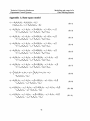
Appendix 1; State space model.
41
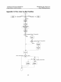
Appendix 2; Flow chart m-file FreeRun.m
.43
Appendix 3; Flow chart m-file PRBNS.m
.46
Appendix 4; Flow chart m-file StairCase.m
49
Appendix 5; Flow chart m-file StepResponseEstimation.m
55
Appendix 6; Flow chart m-file TimeDelayEstimation.m
59
IV
Technical University Eindhoven
Department Control Systems
Modelling and control of a
Glass Melting Furnace
1 Introduction
1.1 Introduction
Efficiency and flexibility are nowadays big issues in the industry. To achieve the high
economic objectives set by the industry all efforts are taken. A part of those efforts is the
advanced control techniques for process control. At the Technical University of
Eindhoven the students can follow a course, applied system analysis (TSA) 5P280, which
give them an introduction in the advanced control techniques. The aim of the course is to
make the students familiar with state-of-the-art model-based, multivariable control
techniques, which are at the moment used in the industry, conceive a test procedure for
developing and validating of the required models and the practical design of a Model
Predictive Controller. The course aims at providing insight in techniques, those are used
for empirical modelling dynamic input output behaviour of multivariable systems with
the use of linear, time invariance, discrete time models and design of those models based
on Model Predictive Control systems.
The students learn to design a test procedure, with which the required models can be
developed and validated in a structured manner. Using the obtained models a Model
Predictive Controller will be designed, within the specifications with respect to the
performance, robustness, and imposed constrains. The simplified industrial case based on
a glass melting furnace is already in existence but in this report the furnace will be
extended with several features. This report discusses the whole model of the glass
melting furnace including the extra features; per-testing of the data and the
automatisation of it in Matlab, with m-files and simulink; furthermore designing and
validating of the model in Inca where the pre-tested data from Matlab is used and the
implementation of it within a data server will be discussed.
1
Modelling and control of a
Glass Melting Furnace
Technical University Eindhoven
Department Control Systems
2 Model of glass melting furnace derived from energy, mass
and momentum equations.
2.1 Introduction
In a glass melting furnace solid raw materials are melted at high temperatures and the
result is a glass melt which then is fined and homogenized. The molten glass contains a
high amount of very small bubbles (containing mostly C02 and N2) and also some solid
materials (mainly Si02) that have to be dissolved in the melt. Furthermore, the glass melt
may not be homogeneous. For the melting of the remaining solid particles it's important
that they have a sufficient long residence time in the furnace at high temperatures along
their trajectories. The small bubbles are released from the melt by letting them grow and
so rise to the surface in the so called hot-spot. This process is called the fining process.
For melting, fining and homogenizing processes not only the temperature is important but
also the velocities in the melt. High velocity gradients give rise to faster dissolution of the
sand grains but on the other hand it may prevent bubbles from reaching the surface due to
high drag forces. In glass melting furnaces several measurements are available, these are:
bottom temperature measurements, crown temperature measurements, pressure
measurements and level measurements. Other variables such as the fining zone where the
release of bubbles take place, the so called hot-spot may be important. The problem is
that the temperature within these zones can not be measured directly. To determine the
temperature in these zones we use an estimator which is designed based on mathematical
models that are available for the glass melting furnaces. Here we discuss the design of
such an estimator for glass melting furnaces based on energy, mass and momentum
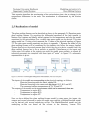
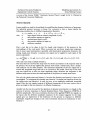
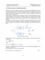
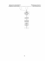
equations models. Figure 2.1 shows a side view of a glass melting furnace with its
measurements.
2.2 Models of the glass melting furnace
Figure 2.1. A side view ofa glass melting fumace with its measurements. IT is temperarure transmitter. PT is pressure transmitter, LT
is level transmitter, PO z is partial ox.ygen pressure and Peo is partial carbon monoxide pressure. The sensor with dotted lines is a
sensor for ox.ygen partial vapour pressure in the melt and it's in a test phase.
2
Technical University Eindhoven
Department Control Systems
Modelling and control of a
Glass Melting Furnace
Glass melting furnaces are often modelled with CFD-codes (computational fluid
dynamics) for design purposes or process operation improvement. Typical and very
important properties of these models are the high level of details and the high
computational effort needed to calculate a solution. These properties are in some cases
important, like control of the glass melting furnace. If a model is used in a controller, it
must allow fast enough calculations and the prediction of the dynamic behaviour in the
important regions must be good enough. The calculations are good enough if it is in the
region of a hundred times real time and the prediction is good enough if the controller
make the process perform within the put performance criteria. Knowing the performance
criteria of the model, one can image that a CFD-code with a very high number of grid
points in general will not live up to these performance criteria of the model. TNO is
putting a lot of effort into developing reduced models derived from CFD-code for
especially glass melting furnaces. Until these models become available testing of
controllers can be done on simple test models derived from first principles or identified
by using input-output from a real furnace. In this chapter a simple model is proposed that
may be useful for:
• Gaining insight in the dynamics of the chemical and physical processes involved
in the melting of glass and their effects on the overall time dependent behaviour
of glass melting furnaces;
• Flexible use which can also be easily extended or simplified and used for:
o The design an testing of controllers;
o Very fast calculation;
• Providing information about variables in glass melting furnaces that are important
for the glass quality.
The model derived is based on furnace 15 of REXAM in Dongen, which is a container
glass melting furnace. This furnace has a single recirculation loop in the glass melt and
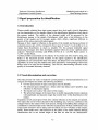
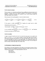
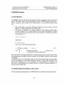
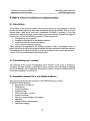
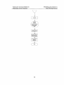
some smaller loops. In figure 2.2 the physical topology of a part of a glass melting
furnace with a recirculation loop is given. The part of the glass melting furnace were the
physical topology of is given is from the inlet of the furnace to the throat of the furnace,
the combustion space with the glass melt beneath it.
(Y~~'k:-2
\.
~
.
I
'' I
I
s,l~
,
BB ••••:············~~3--.
-
I
I
I
'
I'
.
¥s,2
T2--.-n-j
nl
Figure 2.2: Physical topology of a glass melting furnace with a single recirculation loop.
3
Technical University Eindhoven
Department Control Systems
Modelling and control of a
Glass Melting Furnace
As figure 2.2 displays that the glass melt has been divided into 11 regions. Further the
boosting and the environment are indicated within figure 2.2. The physical topology is
based on the method of Prof. H. A. Preisig described in "Modelling of dynamic systems"
1999. Indices used in the physical topology of a glass melting furnace description as
given in table 2.1.
UB
B
NT
T
Under Batch
Bottom
Near Throat
Top
BB
FS
CS
E
Batch Blanket
Fuel Supply
Combustion Space
Environment
Table 2.1: IndIces used m the phySical topology of the glass meltmg furnace.
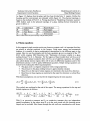
2.3 Main equations
In this approach single monitor points are chosen as outputs, and it is important that they
are placed at relevant positions in the furnace. Using mass, energy and momentum
balances it is possible to derive mathematical descriptions for the different parts in the
system. Here we use the principle and the basic equations given in a preprint of the 15 th
IFAC world congress 2002 Barcelona, title "Estimation of process variable in a glass
melting furnace" by Ir. L. Huisman. For the regions of these models there will be a set of
constants, for the phase boundaries there will be a set of algebraic equations, for lumped,
also called ideally stirred, regions there will be sets of differential equations and for the
distributed systems it will be partial differential equations. Simple energy equations can
be derived by making the following assumptions:
• The glass melt is a singular component with average properties;
• The pressure in the glass melting furnace is approximately constant;
• Mass flows in the top en bottom regions are restricted to the main flow direction;
• Heat flows in these regions are restricted to the main flow direction a vertical flow
direction.
With these assumptions one can find for the lumped regions the next equation:
(2.1)
The symbols are explained at the end of the report. The energy equations for the top and
bottom regions are as follows:
With ~l as convective transport and ~2 as conductive transport they are independent
spatial coordinates. In the source term Se or in the work terms UIWI the boosting power
(input) can be included. Heat losses through the side walls are considered as sink terms.
4
Technical University Eindhoven
Department Control Systems
Modelling and control of a
Glass Melting Furnace
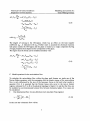
Discretization of the spatial domain the energy equations, equation 2.2, are transformed
into a set of ordinary differential equations (ODE).
The temperature description will be completed if the mass flows between the system
regions are known. If the assumption is made that the pull rate is approximately equal to
the furnace load (due to the presence of a level controller) then only one mass flow is still
unknown. This unknown mass flow can be expressed as the ratio, R
=
?T
Vpull
,of the glass
flowing back to the batch blanket (upper regions flow) and the pull rate. Glass flows in
the regions can be described with the Navier-Stokes Equations, a microscopic momentum
balance. By taking the dot product of the velocity vector v with the Navier-Stokes
equations and integrate the resulting equation over the glass melt volume yields:
with
E !,;
K =!!:..- n..!.. pv2
101
dt !l2
=- f(r : Vv)do.
)do.
the total
kinetic energy in the
glass melt and
the friction losses from the laminar flow patterns that are assumed
Vi
in domain part i, where also the assumption is made that it only occurs in the top en
bottom regions. If the assumption is made that the kinetic energy varies due to changes in
the buoyancy forces in the melt only, then:
(2.4)
Due to temperature differences in the melt this equation approximates the acceleration of
the glass in a recirculation loop.
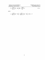
2.4 Equations parts glass melting furnace
A. Heat transfer in laminar flow regions.
For the laminar flow regions in the tank we can use a two dimensional model, therefore
we can use the equation (2.2) for the calculations. But first we have to discretize the
energy equation into the next equation which we can implement:
5
Modelling and control of a
Glass Melting Furnace
Technical University Eindhoven
Department Control Systems
(2.5)
Here, a central difference interpolation scheme for the diffusive terms and an upwind
scheme for the convective terms are applied. For the top flow three regions are taking and
indexed along the flow direction, for the first region we get (upper right):
(K
K
eff
dTTl _
1
(T +T )- eff (T +T
dt - pC pt:.~l t:.~l T2
Tl
t:.~1 Tl
NT
+
pC
1
(K---.-.:!!....
pt:.~2
t:.~2 T
(813
+T
Tl)
K
t:.~2
)J
/
----.-.:!!.... T +T
(Tl
J
S,Tl)
(2.6)
_(V1)(T +T )+WbSI,Tl+ qTlIE
j:
t:.~1
Tl
NT
pC p
pC p V Tl
For the first of the middle regions we similarly get:
(2.7)
We can find similar relations for the other bottom regions.
B. Ideally stirred regions.
The region under the batch blanket is an ideally stirred region and an energy equation for
a constant pressure zone can therefore be used:
6
Technical University Eindhoven
Department Control Systems
dTUB
pC PVUB ---;Jt = pCp VqUB Tn A
Modelling and control of a
Glass Melting Furnace
(
BBI
A
-Vpull<l> BB
)
TUB
p~RH
(2.8)
-aeffAUBIBBI (TUB - T BBI )
Awall AUBlE (T. _T
owall
UB
)
E
The degree of mixing in the UB-region, which has an effect on the heat transfer
coefficient <lerr , is indicated with YUB. Further more is assumed the chemical reactions
take place outside the UB-region and the glass is treated as a single component having
average properties that depend on the composition of the glass.
The region near the throat can be modelled similarly with:
pC pVNT
dTNT
---;Jt
= pCp VB13INT
A
(
TB13 - TNT
)
+pC pVB 231NT (TB23 - TNT)
(2.9)
-aeff,NTACSINT (TNT - TE)
- AwallANTIE (TNT - T )
E
°wall
C. Model equations for the recirculation flow.
To calculate the recirculation flow within the glass melt furnace we make use of the
Navier-Stokes equations with the assumption that the kinetic energy of the recirculation
flow is only influenced by the size of the buoyancy forces in the melt what results in
equation (2.4). It is assumed that the friction losses only occur in the top en bottom
regions, indicated by T en B in the physical topology in figure 2.2, and that the flow can
be modelled as one dimensional laminar flow between horizontal plates. Two cases can
be considered:
•
One dimensional flow (in one-direction) over one plate (Top-regions):
(2.10)
In this case the volumetric flow will be:
7
Modelling and control of a
Glass Melting Furnace
Technical University Eindhoven
Department Control Systems
v. = fM(~.t=2
-H.t= )dQ= -WM
H
f.1L 2
3f.1L
3
~2
I
~2
I
Ai
and so
8
(2.11)
Technical University Eindhoven
Department Control Systems
•
Modelling and control of a
Glass Melting Furnace
One dimensional flow between two plates (Bottom-regions):
J-
J.
;::
;:: WIth Yi =6
H';.2
= - -yjY;
3 (1;::2
-Y;';.2 - H';.2
2j.1L 2
WH j 6
The accumulation term from the velocity profile can be written as:
VI
with R
j:2 =-MJ- (1-';.2
K rc
=
=
;T
1 2
1 2) 1 V y2
( 60 Yn + YTI 2" p T pull
y 2pV y 2
dR
--'---:-----':
R + B B pull (R + 1) _
WT2H T2
60WB2H B2
dt
15
(2.12)
(2.13)
a dimensionless backflow ratio and y a constant depending on the
V pull
situation (one or two plates). For the friction we can derive:
E
"2
J,TI
= 3VT J1Lr1
W H3
T T
E
'J.T2
"2
= 12VT J1Lr2
W H3
T T
and E
"2
J,B
= 12VBj.1LB
W H3
B B
(2.14)
and the buoyancy terms can be written:
(2.15)
Using the equations (2.4), (2.13) and (2.15) we rewrite the kinetic energy equation and so
obtain a nonlinear equation for R:
dR
dt
=
1 2
1 2)1
2
( -Yn +-YTI -pVT
60
15
2
y2 R+ YBPVB y2 (R+l)
W 2H 2
pull
60W 2H 2 pull
T
T
B
B
(2.16)
1 2
1 2)1
2
( -Yn +-YTI -pVT
60
15
2
y2 R+ YBPVB y2 (R+l)
W 2H 2
pull
60W 2H 2 pull
T
T
B
9
B
Modelling and control of a
Glass Melting Furnace
Technical University Eindhoven
Department Control Systems
This equation describes the acceleration of the recirculation glass, due to change in the
temperature differences in the melt. The acceleration is counteracted by the friction
forces.
2.5 Realisation of model
The glass melting furnace can be described as shown in the paragraph 2.4 Equations parts
glass melting furnace. By rewriting the differential equations of the heat transfer in
laminar flow regions and ideally stirred regions for the temperatures and also the model
equations for the recirculation flow a usable state space model can be derived. This state
space model has 12 states which represent the 12 states of the physical topology of figure
2.2.The state space model equations are shown in appendix 1. Because the model of the
glass melting furnace will be considered by the students who follow the course Applied
System Analysis as the actual process from which they have to derive a model from, the
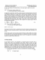
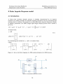
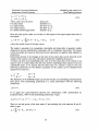
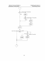
glass melting furnace has to be as realistic as possible. Disturbances at the inputs and
white noise with spikes at the outputs can make the model more realistic, as almost all
industrial processes are corrupted with these types of "noise", in figure 2.3 a schematic
representation is given.
Input
Disturbance
Inputs
1
I
I
White Noise
+
+
~
~
Spikes
+,
~
I
Model
+
+
+
~I
Outputs
I
Figure 2.3: Schematic of model of glass melting furnace with disturbance. white noise and spikes.
The inputs of the model are corresponding to the physical topology as follows:
Electrical boosting under the batch, region UB;
Electrical boosting in the centre and near throat, B12, B13 and NT;
The connected surface temperatures ofTl, 1'2 and NT.
The outputs of the model are the temperatures which can be measured; these are:
Temperature in region B21;
Temperature in region B22;
Temperature in region NT.
Now we have defined the glass melting furnace model by state space, the inputs, the
outputs and several elements to make the model more realistic a Matlab/Simulink model
can be derived with several underlying m-files. The Matlab/Simulink model and the
underlying m-files can found on the cd-rom in the directory "course TSA
10
Technical University Eindhoven
Department Control Systems
Modelling and control of a
Glass Melting Furnace
software\Matlab Simulink" subfolders "Simulink files" and "TSA m Files lower level"
which is included in this report.
11
Modelling and control of a
Glass Melting Furnace
Technical University Eindhoven
Department Control Systems
3 Signal preparation for identification.
3.1 Introduction
Process models obtained from input output signals have their quality heavily depending
on the characteristics of the signals offered to the identification algorithms which derive
the process models. The quality of the obtained model will be governed by the
disturbances present in the signals. Disturbances which have a bad influence on the
quality of the models are for example: spikes, drifts, offsets, significant different in
powers of the various input and output signals.
Because of their negative influence on the quality of the models and because almost all
industrial process data will be corrupted by these types of "noise" it's advisable to try to
reduce these disturbances as much as possible. For this purpose dedicated signal
processing techniques have been developed, applied within the course "applied system
analysis", Technical University code 5P280, of Prof. dr. ir. A.C.P.M. Backx and dr. ir.
AJ.W. van den Boom.
Another problem encountered in the industry is the present of, often relative long, time
delays in the measured process transfers. If the signals applied to the identification
algorithms are not corrected for these time delays, the delays have to be estimated by the
algorithms. In most cases this implies many extra parameters, corresponding to these time
delays, have to be used for the modelling. This too has a deteriorating influence on the
quality of the models ultimately obtained.
3.2 Trend determination and correction
The (sub) process one wants to model for control purposes is mostly determined by a set
of inputs and outputs that satisfy the following conditions:
• On-line measurement of inputs and outputs must be feasible;
• The selected inputs should have a direct (short time delay) and if possible, large
influence on the process outputs;
• The inputs have to allow full control of the outputs;
• The permitted changes of the inputs have to enable measurable process responses
with amplitudes and dynamic ranges that exceed those of the disturbances in the
outputs.
In general, not all actual inputs which have a direct influence on the outputs are selected.
The inputs that not have been selected for the modelling may, however, contribute to the
changes found at the outputs of the (sub) process. During the modelling these changes are
considered as coloured output noise. Often the characteristics of these contributions to the
output noise are known and in many cases the effects are slow variations of the outputs:
trends. These trends have a bad influence on the quality of the model obtained through
identification due to the limited length of the data set used for the identification.
12
Technical University Eindhoven
Department Control Systems
Modelling and control of a
Glass Melting Furnace
To show the influence of the limited data set, the output signal is split into two parts:
Y = Yp + ~r
with:
Yp the process outputs without trend
Y tr the trend signal added to the process outputs
An approach to separate the trend from a signal is based on the determination of the trend
by filtering the signal with a low pass filter and subtraction of the obtained trend from the
signal. However, filtering of a signal with a low pass filter introduces a phase shift
between de original signal and the obtained trend signal. Subtraction of the two leaves
unwanted signal components in the corrected signal. To overcome this phase shifting
problem, the signal can be filtered twice: once with a causal low pass filter en once with a
corresponding anti-causal filter. The average of the sum of the two filtered signals
obtained will not be shifted in phase any more compared to the original signal. This can
be mathematical expressed:
-1
00
00
~rt = LhtYk-i + LhtcYk_i = Lhi Yk-i
;=0
;=-00
(3.1)
i=-o<J
hC the causal filter impulse response
hac the anti-causal filter impulse response
with:
and h
C
I
= hac for 1<i<oo
-I
-
The design of the filter will be a compromise between the demands, determination of the
trends as accurate as possible and that no relevant process output signal information will
be lost.
Beside trends, signals can have other unwanted characters, offsets. Offsets have almost
the same influence on the estimated parameters as a trend has. The offsets in the signals
are assumed to be signal values that are constant in time. The changes due to the process
dynamics are added to these offset levels.
3.3 Peak shaving
In the industrial practice is the disturbance of measured signals with spikes often a
problem. This is due to the amplitude of those spikes which are mostly very large
compared with the signal changes obtained from the process. Most of the time the spikes
last from one sample to sometimes tens of samples. Considering that spikes are an
important part of the noise energy they can have a great influence on the ultimate model
although they have no relation with the process themselves. Therefore it is wise to
remove the spikes as much as possible. This can be done in the following four steps:
• Clip the signal amplitudes to values never reached by the real process signals:
Sk
=
with:
tel .
(3.2)
Sk
Sk
the clipped signal
13
Modelling and control of a
Glass Melting Furnace
Technical University Eindhoven
Department Control Systems
the measured signal corrupted with spikes
Sk
•
Compute a trend signal from the clipped signal:
k
Sk
= Ihlsk- I
(3.3)
I=k-I
•
Compute the standard deviation of the trend-corrected, clipped signal:
•
(3.4)
1 1=0
Interpolate all samples of the original signal that are outside the band which can
be defined as a· standard deviation. The permitted signal band is given by:
Sk + a· S
upper limiet
S
~(_SI - -)2
=-1 L..J
SI
xk
=
{
a· S
lower limit
All consecutive sample values that are outside the permitted band are replaced by
values obtained from a linear interpolation starting from the least accepted sample
value and reaching to the first next sample value within the permitted band after
the spike.
The multiplication factor a has to be chosen such that no process signal values are outside
the permitted signal band. With this method the noise energy caused by the spikes is
reduced significantly and because of the interpolation the signal is kept at an average
process signal level where at those sample moments no real process information is
available. Using this signal treatment the influence of the spikes is reduced to a negligible
level.
Sk -
3.4 Estimation of time delays
Measured process responses can contain time delays. If those time delays are not
corrected, they become a part of the estimated process model. Although they are a part of
the model, the time delays do not contribute to the further dynamic behaviour of the
process. Because the time delays involve extra model parameters (one extra Markov
parameter for each delay sample) the number of parameters to be estimated increases
when the modelling of the time delays has to be done by identification algorithms. When
the time delays are not corrected, the parameters increases and so the computational
effort required for the modelling of the process which therefore decreases the expected
accuracy of the model.
14
Technical University Eindhoven
Department Control Systems
Modelling and control of a
Glass Melting Furnace
A good approach to overcome this time delay problem is estimation of the time delays
separately from and prior to model parameter estimation. The information obtained can
then be used as a-priori knowledge to correct the measured process signals for these time
delays as much as possible. When the estimated model is obtained, the time delays can
then easily be included into the model.
Estimation of time delays in process input/output transfer can be done with correlation
techniques. One method is based on the analysis of the cross-correlation between input
and output signals. The assumption is made that the process is ergodic, the input signal
applied to the process is stationary, white, inter-channel independent, zero mean noise
se9uence with covariance matrix R:
Etu . u l
}= R =a 2 [
(3.5)
p
Then the autocorrelation function of the input signal becomes:
{a
1 ~
I _
l' =0
_ I'Im--·L.JuiU,ui[ p
(3.6)
H= 1 + 1 i=O
0
l' '" 0
Furthermore, if the input signal is assumed not to be correlated with the output noise and
using the properties of the input signal u, the following expression is obtained for the
cross-correlation between outputs and inputs:
=
1
1
=
(3.7)
'If yu (1') = lim-·
jUk+iU-j . U~+i + 'lf nu (1') =
j'lf uu (j -1')
j=O 1-+= 1+ 1 i=O
j=O
In equation (3.7) the parameters Mj are the elements of the process impulse responses
including the time delays. Substitution of equation (3.6) into (3.7) gives:
2
'If yu (1') = a M T
(3.8)
Consequently the cross-correlation function obtained will have the shape of the impulse
responses in case the input signal is a stationary, white, inter-channel independent, zero
mean noise sequence. Otherwise the cross-correlation function is convolution of the
impulse responses with auto-correlation function of the input.
'lf uu (l' ) -
I
2
IM
IM
The actual time delays can be found from the cross-correlation function by looking for
the beginning of a sequence of values that differ significantly from zero. The first
element of that sequence is the time delay.
3.5 Basic assumptions
Basic assumptions have to be made to derive a model from input output data, these are;
Process is linear;
Process is time invariant;
Process behaviour can be approximated by a finite complexity;
Process is causal;
Manipulated variables enable within their available operating range.
Without these basic assumptions it's not possible to derive a suitable model which allows
fast enough calculations and the good enough prediction of the dynamic behaviour in the
important regions. These basic assumptions can be derived and tested on the process this
15
Modelling and control of a
Glass Melting Furnace
Technical University Eindhoven
Department Control Systems
is a part of the Course 5N060 "Stochastic System Theory" taught by Dr. S. Weiland at
the Technical University Eindhoven.
Test for linearity
Linear models are used in the methods for modelling the dynamic behaviour of processes.
No industrial process, however, is linear. For a process to have a linear transfer the
following condition has to fulfilled (superposition theorem):
u\ ---7 Yl and U z ---7 Yz ~
a· u\ + f3. U z = a· Y\ + f3. Yz
with UI
-input signal with an arbitrary amplitude (UffO);
YI
-the process response to input UI;
U2
-second input signal (U2:fO);
Y2
-the process response to input U2;
a,~
-arbitrary constants.
First a test has to be done to test for steady state linearity of the process in the
surroundings of the work point. When a process has non-linear steady-state responses
then in most cases linearization is possible with linearization polynomial functions. For
testing steady-state linearity a staircase test signal can be applied to each input of the
process separately:
s
Uk
= a e ZJu(k -i ·-r)-u(k -(s + 1+i)·-r)-u(k -(2s + 2+i)·-r)+u(k -(3s + 3+i).-r)] (3.9)
i=O
with: uG) a unit step at sample moment j.
The time interval 't between the steps most be chosen accordance to the response time of
the process. By each step applied the process most reach a steady-state, then a steadystate analysis can be done properly. The maximum amplitude of the test signal has to
exceed the amplitude range that has to be covered by the model. Each step of the stair
case test signal has to have an equal amplitude range; therefore the responses to the
different steps need to have the same amplitude if the process is steady-state linear.
Not only the steady-state non-linearity's but also the dynamic non-linearity's have to be
investigated. To investigate the dynamic non-linearity's a similar test based on the test for
the steady-state non-linearity's is used, but now as an amplitude modulated sinusoidal
signal. Here the test signals consists of different frequencies of the wave carrier, thus it
gives an insight in the non-linearity's at different frequencies.
Another test that can be used for the detection of dynamic non-linearity's is based on the
analysis of process responses on Pseudo Random Binary Noise Sequences (PRBNS) of
different amplitudes. The cross-correlation function of the applied PRBNS test signals on
the inputs and the different amplitude responses of the outputs triggered by the input
signals give an impression of the behaviour of the process in response to different
amplitudes. Significant changes in the cross-correlation function are indications of nonlinearity's.
16
Technical University Eindhoven
Department Control Systems
Modelling and control of a
Glass Melting Furnace
Test for time invariancy
Time invariancy is an important specification from modelling the dynamic behaviour of
processes. A process can not be correctly modelled if the behaviour of the process
changes as a function of the time. For a process to have a time invariant transfer the
following condition has to fulfilled:
The state space of the model (appendix 1) can be rewritten towards:
(3.10)
If the process is stable then
R(:')[;] ~ 0,
therefore the model must be stable
(disregarding numerical errors).
By selecting p =ker
R(
we can conclude tbat:
:J ~ [;}/) P [;}t+
R(
E
then
:J[;}t) =
0 for \I
r) E
p,
I, so R( :1)[;}I +
r)
~0
and tberefore
the process and model, are time invariant.
Test for causality
A signal is causal if f(t)=O for t<O. So if we rewrite the state space of our model to the
form: i = A! + lffi, Y = c T ! + du and we consider a causal input signal and the model is
linear then the response of the model for t<O on the causal input signal, which for t<O will
be a zero-input-signal, can only be a zero-output-signal. So a causal input signal will
produce a causal output signal and therefore the model will be causal. This can simply be
tested by using a causal input signal, for example a step.
3.6 Realisation of signal preparation
The realisation of the signal preparation will be done by several special written m-files in
Matlab combined with a simulation in Simulink. With these m-files a total of five several
simulations can be chosen for the signal preparation, these are:
Free run test;
Delay time test;
Step response test;
17
Modelling and control of a
Glass Melting Furnace
Technical University Eindhoven
Department Control Systems
Stair case test;
Pseudo Random Binary Noise Sequence (PRBNS) test.
To run the m-files, two low pass filters have to be designed with the tool "fdatool" of
Matlab. Within the m-files the output data can be filtered with those filters at a causal and
anti-causal manner. This prohibits an extra phase shifting problem. A proper design of
the two filters will eliminate the spikes for an important part therefore the remaining
noise energy in the spikes will have a limited influence on the to devise ultimate model of
the students. At this point the model as described in "Model of glass melting furnace
derived from energy, mass and momentum equations" will be considered as the process.
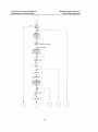
With the free run test, m-file "FreeRun.m" the drift per time unit of all the process
outputs can be measured.
The m-file "DelayTimeCalculation.m" all the time delays of the process in relation to the
selected input and al the outputs can be estimated through cross correlation of the input
signal and output signals.
The step response of the process in relation of all the inputs and outputs can be estimated
with a first order response fitting, y(l)
~ Gain x ( I - e -,,-;-,) Jthrough
the m-file
"StepResponseEstimation.m".
The gain, tau and the time delay, together with the found time delay,
"DelayTimeCalculation.m" can be estimated and/or checked.
as
the
m-file
The
m-file
"StairCase.m"
has
the
same
features
"StepResponseEstimation.m" except now a staircase signal is used, where all aspects
such as time per stair, number of stairs of incurring slope and amplitude per stair will be
designed by the user. A logical consequence is that the selected output response will be
estimated per stair response by a first order response fitting describes as above. This will
give the user an extra insight in the linearity of the process within its designed work area.
The Pseudo Random Binary Noise Sequence (PRBNS) test done with m-file "PRBNS.m"
there the user is allowed to extract, with a designed PRBNS signal for all the inputs, the
responses of the outputs of the glass melting furnace process. The user has the possibility
to design the PRBNS input signals by selecting the time of the PBRNS signal per input,
the maximum amplitude of that signal per input and the switching probability of the
PBRNS signal per input.
All the m-files will store the data of both the inputs and the outputs with the actual real
time per sample in such a way that it can be used as process data for obtaining a model of
the glass melting furnace process with the Modeller of Inca.
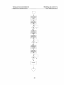
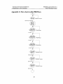
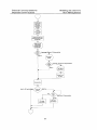
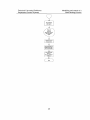
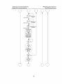
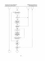
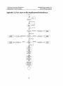
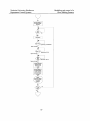
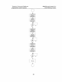
Flow charts of the m-files can be found in appendix 2 to 6. Of course all parameters to
run the m-files and the process, the glass melting furnace model within Simulink, are all
ready preset through the usage of the m-files.
The actual use of the m-files including the filter design is discussed in the manual "User's
Manual customized software" which can be found on the cd-rom included with this
report in the directory "course TSA software\Installation Information Files". Within this
manual the filter design, the filter properties, all the m-files and properties of all the mfiles are discussed. With this manual the students who follow the course TSA will have a
guideline to derive and prepare the data from the process, the glass melting furnace
18
Modelling and control of a
Glass Melting Furnace
Technical University Eindhoven
Department Control Systems
model within Simulink. Also through the usage of the m-files derived and prepared data
will automatically be rewritten into the needed structure for use in the application
"Modeler" which will be discussed later on in this report.
19
Modelling and control of a
Glass Melting Furnace
Technical University Eindhoven
Department Control Systems
4 Finite Impulse Response model
4.1 Introduction
A linear time invariant dynamic process is uniquely characterized by its impulse
response. For stable processes, the impulse response will tend to zero for increasing time
and may then be reduced. This results in so-called FIR (Finite Impulse Response) models
or Markov parameters. For SISO (Single Input Single Output) process such a model is
given by:
N
y(t)=gtu(t-l)+g2u(t-2)+ ... +gnu(t-n)=l..gju(t-i)=rp(t)B
;=1
In matrix form :
y
= rjJB
(4.1)
andrjJ=[u(t-l)
u(t-2)
...
u(t-n)]
gn
By introducing the residual as: y = rjJB + E in matrix form,
where:
u(n -1)
E(n + 1)
u(n)
yen + 1)
y=
yen + 2)
E=
E(n+2)
and rjJ =
E(N)
yeN)
u(l)
u(n+l)
u(N)
u(N -n)
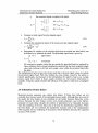
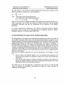
Figure 4.1 shows the block diagram of a FIR model estimation of a SISO process.
v(t)
+
U(t)
y(t)
Process
U(l-I)
£(t)
Figure 4.1: error generation in FIR model estimation.
20
Technical University Eindhoven
Department Control Systems
Modelling and control of a
Glass Melting Furnace
Figure 4.1 gives us the output error of the misfit of the model compared to the process.
With the least square method we can estimate the parameters of the model. First we
calculation the sum of the squares of the simulation error or output error:
1 ~ £OE ()2
= -LJ
t
VOE
(4.2)
A
N
1=1
So we can find the minimum of VOE through:
dVOE = 0 with i = 1...n
dg
(4.3)
j
The minimum of equation 4.3 give us the best fit of the model on to the process so with
computer assistance the parameters of the FIR-model can be calculated.
The order of the FIR model has a direct influence on the error generation, Furthermore;
noise on the signals can cause randomness in identified models. One can calculate the
order of the FIR model through several mathematical theories or one can use the practical
fist-rule: "The order of FIR-parameters is approximately equal to the time to steady state
divided with the sample time".
FIR models have several advantages and disadvantages, these are as follows:
Advantages:
• Less a priori knowledge of the process is required to estimate a FIR model. Only
the order of the process is required;
• FIR model estimation is statistically unbiased, the expectation of the estimation
equals the true values, and consistent, the estimation tends to the true value when
a number of data points to infinity.
Disadvantages:
• The FIR model often needs to have a larges number of parameters; the estimated
process is not accurate for a finite number of data. The inaccuracy has to do with
the variance of the estimation which is proportional to the number of parameters
of the FIR model;
• A FIR model is often not suitable for linear control design methods due to the
reduction of the very large FIR model.
The extension of the FIR model estimation to multivariable processes is straightforward
in the same way as with a single variable process, described above. The generalization of
the difference equation model leads to a so called matrix friction description (MFD). In
general, parameterisation of MIMO MDF models for identification is a complicated
problem this will not be discussed in this report.
21
Technical University Eindhoven
Department Control Systems
Modelling and control of a
Glass Melting Furnace
4.2 Order selection, a simulation approach
In practice, the order of a process is seldom exactly known. Order selection should not be
confused with model validation. Model order determination is an imported part in the
process identification. Here we present a simple but effective technique to estimate the
order of the process. The order of the FIR model is related to the time to steady state of
the process or the settling time.
Order selection is nothing more then finding a model order that best explains the given
process data. Here the task of model validation is necessary to check whether the model
is good enough for the intended use. A model derived from data can give the best
possible fit to that data, but that model doesn't have to be the best model for using
purposes.
A method for validating a model is to simulate the estimated model using some real input
data of the process and comparing the output of the model to the real output data of the
process. In figure 4.2 (next page) a schematic representation of this model validation is
given.
vet)
+
yet)
+
Process
+
u(t)
Model
ym:xlel(t)
Figure 4.2: Order selection by simulation.
The goodness of the fit is measured by the sum of the squares of the simulation error or
output error:
1~
)2
VOE =-~COE(t
N r;l
where
(4.4)
A
A
CoE(t) = y(t)-
B(q-l)
A
A(q-l)
u(t) = y(t)-YmOdel(t)
Note that we are discussing here the FIR model so A(q)=l therefore the equation error is
equal to the output error.
For order selection we can use the output error:
(4.5)
22
Modelling and control of a
Glass Melting Furnace
Technical University Eindhoven
Department Control Systems
Thus the error consists of the model misfit and the output disturbance. By looking at the
formula for V OE we can conclude in general that the loss function decreases as the order
of the model increases. For estimating de order of the model we only have to look at the
reduction of V OE when increasing the order of the model. As long as the reduction is
significantly, it is worthwhile increasing the order of the model. Of course the model
validation should not be done on the data set which has been used to estimate the model,
because a good fit of the model on that data set will not prove sufficiently the model
quality.
23
Modelling and control of a
Glass Melting Furnace
Technical University Eindhoven
Department Control Systems
5 MPSSM model
5.1 Introduction
An MPSSM (Minimal Polynomial Start Sequence Markov) parameter model is estimated
from a FIR model. There are two advantages of using a MPSSM model compared to a
FIR or a (pseudo) conical model for the identification of a multivariable process, these
are:
•
•
The model doesn't need any information about the systems structure, just the
degree (r) of the polynomial has to be determined;
The number of parameters of a model of degree r with p inputs, q outputs and a
D-matrix equation (5.1) is small compared to the number of parameters nj needed
for the description of the dynamics of the same systems of its Markov parameters
only equation (4.1):
nm
= (r + 1) . p . q + r
respectively:
n i = (m + 1) . p . q
with r: order of the minimal polynomial.
Yk
= :tF;(aj,mjV£I~k_l
1= 1,2, ..... r
(5.1)
;=0
ith Markov parameter
dim(FD=q x p.
lh coefficient of minimal polynomial.
Following the first advantage, difficulties with determination of the structure indices from
the measured process signals which are required for the MIMO (pseudo) conical models
are avoided.
A MPSSM model can be determined directly from the measured input and output data.
For the computation of the model parameters, however, a high order function of the
polynomial coefficients have to be minimized. For the mathematical explanation, we
refer you to "Identification of an Industrial Process: A Markov Parameter Approach" of
professor Backx dated 1987.
5.2 Mathematical description of the system
For the mathematical description of a MPSSM model we introduce a state space model:
24
Modelling and control of a
Glass Melting Furnace
Technical University Eindhoven
Department Control Systems
Xk+1 = F 'X k + G 'U k
Yk = H . Xk + D· Uk
with Xk state vector at time k
F is state matrix
G is input matrix
H is output matrix
D is direct feed through matrix
(5.2)
dim[xkl=n;
dim[F]=n x n;
dim [G]= n x p;
dim [H]= q x n;
dim[D]= qx p;
From this state space model we can derive a description of the input output behaviour of
the system:
k
Yk =H·Fk·X0 +"H·Fi-I·G·u=D·u
L..J
k-l
k
k~O
(5.3)
i=1
with Xo the initial vector of the state vector.
The model is assumed to be completely controllable and observable. In general, models
obtained by process identification techniques will be completely observable. The reason
is that the models are based on observed process response(s) on applied input signal(s) to
the process.
Information present in the changes of the state of the system that can be observed at the
outputs of the system is the only information needed for modelling the process.
A system can have non-controllable parts, such as if the initial state of the system is not
equal to zero or if other inputs then the ones used for modelling (noise inputs) excite non
controllable states. If we assume that the initial state of a system is equal to zero, the
following expressions for the Markov parameter of the system can be obtained from
equation (4.1) and (5.1).
D
gi= { H.Fi-I
fori = 0
fori>O
The definition of the MPSSM model can be derived after an annihilating polynomial has
been given. This annihilating polynomial is a scalar polynomial with the following
satisfaction:
f(F)
=0
(5.4)
If we apply the Cayley-Hamilton theorem (ref. Gantmacher, 1959, implemented by
professor Backx, 1987) in the annihilating polynomial, we get:
There we use the power of the state matrix F and multiply this with matrixes Hand G,
there we get:
n
gj
= L -ai ·m j _i
for all j > n
(5.5)
i=1
25
Modelling and control of a
Glass Melting Furnace
Technical University Eindhoven
Department Control Systems
The state matrix F also satisfies its minimal polynomial, the recurrence relation for the
Markov parameters, equation (5.5), can be reduced to:
r
mr +j
= L - ai • m r +j - i
i=1
with
r the degree of the minimal polynomial;
aj the coefficients of the minimal polynomial;
m r+j = mr+/ai'mjlieI)
1= 1,2,3, ... ,r
Now we can see that a complete description of the system only requests the first row r
Markov parameters, the so called start sequence of Markov parameters, and the minimal
polynomial coefficients that give the continuation of the sequences of the Markov
parameters.
For further mathematical underlying of the Minimal Polynomial Sequence Markov
parameters model we refer you to "Identification of an Industrial Process: A Markov
Parameter Approach" of professor Backx dated 1987.
5.3 Determination the degree of the minimal polynomial
The determination of the degree of the minimal polynomial has to be done on the basis of
the available input/output data and/or with already estimated Markov parameters. In de
industrial practice, the process in general does not fit in the model set so that's a problem
with the determination of the degree of the MPSSM model. The choice of the degree r for
MPSSM models simply has to be based on considerations with respect to the ability of
the models from that model set to simulate the measured process behaviour with certain
accuracy. In industrial identification practice the model is not constructed on the basis of
a theoretical knowledge of the process dynamics due to the complexity of the processes.
Therefore, no direct relation can be found between the process to be modelled and the
degree (r) of the model.
In practice two different approaches are used for determination of the degree (r), these
are:
• Several models with different degrees of (r) are estimated and compared to the
measured process behaviour in relations to output errors of the several models and
the process;
• From the estimated sequence of Markov parameters consisting of the main part of
the process impulse responses and order are determined by looking for the most
dependences between the estimated parameters.
The output error of the first approach is constructed in the same way as with the FIR
model en therefore the schematic representation of figure 4.2 (order selection by
simulation) can be applied.
26
Technical University Eindhoven
Department Control Systems
Modelling and control of a
Glass Melting Furnace
6 Model realisation
6.1 Introduction
At this point we have discussed the process, signal preparation for identification and two
different types of models. Here we discuss the realisation of a model derived through the
use of the treated, prepared signals and the use of "Modeler", an application of IPCOS
technology. Through the use of the application "Modeler" there will be the option to
derive a total of four different models, namely:
• Finite Impulse Response;
• Equation Error;
• Output Error;
• Subspace.
The students who follow the course TSA have been given the process as described in
chapter 2_, "Model of a glass melting furnace derived from energy, mass and momentum
equations and have treated, prepared the signals through the use of the m-files discussed
in chapter 3, "Signal preparation for identification".
6.2 The variables
The variables used to derive a model from the process are already preset. This is because
the assignment for the students who follow the course TSA is already in existence before
the expansion and modification of the assignment and there for the "red line" of the
assignment has been followed as it was. We can divide the variables into two mean
categories, namely input variables and output variables also called manipulated and
controlled variables within the application "Modeler". These variables can be further
more divided:
• Input variables
o Electrical boosting under the batch, region UB; This variable has the
dimension Watt.
o Electrical boosting in the centre and near throat, B12, B13 and NT; This
variable has the dimension Watt.
o The connected surface temperatures of Tl, T2 and NT. This variable has
the dimension Degree.
• Outputs variables
o Temperature in region B21; This variable has the dimension Degree.
o Temperature in region B22; This variable has the dimension Degree.
o Temperature in region NT. This variable has the dimension Degree.
The different regions, addressed with the variables, are visualised in figure 2.2, chapter
"Model of glass melting furnace derived from energy, mass and momentum equations".
27
Technical University Eindhoven
Department Control Systems
Modelling and control of a
Glass Melting Furnace
The input variables are the changes on to the process set point and the output variables
are the actual temperatures within the glass melting furnace.
6.3 Modeler; the application
Model is an application of IPCOS technology where models of a process can be obtained
through the usage of data derived of logging the process variables. As described in the
previous sub-chapter the variables are known and with the usage of the m-files all needed
data of the signals is already present, prepared and in the right structure for Modeler.
For the students who follow the course TSA a manual has been written, "Coordinating
User's Manual" where the outlining of Modeler and the usage of Modeler are described.
The description of the usage of Modeler is only to point the students in the right direction
and so student will have to develop the model also with the usage of the manual of
Modeler which is on the installation cd-rom of the IPCOS products. The level of
accuracy of the obtained model is depending on the students affords to derive the correct
model from the data. This means students can not use only the information in of the
manual "Coordinating User's Manual" to derive the correct model. The "Coordinating
User's Manual" can be found on the cd-rom included with this report in the directory:
"course TSA software\Installation Information Files".
28
Technical University Eindhoven
Department Control Systems
Modelling and control of a
Glass Melting Furnace
7 Software architecture
7.1 Introduction
For the implementation of the glass melting furnace model in Simulink in a software
environment with the Model Predictive Controller (MPC), this software environment
with a number of different software applications must be developed. This environment
enables easy transfer of the data between the software applications. Through the software
environment with a preset of the applications, which must be a standard, the students who
follow the course TSA can easily implement their model and develop their controller on
the basis of MPC technology.
This chapter describes the application architecture, the software application used in the
environment, the used configuration files for the software environment and the preset
standard used for the environment with the standard for the applications.
7.2 Application architecture
The application architecture used to apply the MPC to the glass melting furnace model in
Simulink is visualised in figure 7.1. In this architecture the MPC uses the model
developed by the students. The students must develop the model with data derived
through the signal preparation files, see chapter 3, within the INCA application "Model".
The glass melting furnace model in Simulink will be actual the process for the students.
Scheduler
Matlab
Simulink
1+---+1 Data Server 1+---+1 INCAengine
INCAtest
INCAview
figure 7.1: Application architecture
The different applications within figure 7.1 will be briefly discussed:
29
Modelling and control of a
Glass Melting Furnace
Technical University Eindhoven
Department Control Systems
Data server:
The INCAdataserver software form IPCOS Technology is a software program that serves
as a gateway for process data. The data server connects the different applications to the
glass melting furnace model, the actual process.
Scheduler:
The scheduler triggers the different applications to an active status in a defined sequence.
The sequence as shown in figure 7.2 is the sequence used in the scheduler for the
application architecture design for the course TSA.
figure 7.2: Scheduler sequence.
Matlab/Simulink:
With Matlab a Simulink: model of the glass melting furnace will be runned through an mfile every time Matlab is triggered. Simulink is an application of Matlab. The model of
the glass melting furnace is here considered as the real process including the futures of a
real process such as spikes.
INCAtest:
INCAtest is an application of the IPCOS technology used for logging and testing data.
This application will enable visualisation of the signals present in the data server and
logging of those signals. The logging of the data can be done in an ASCII format thereby
simplifying the use of data within other applications for analyses and modelling.
INCAview:
The application INCAview of IPCOS technology visualises the variable present in
INCAengine. The students can use this application for performance check of their
developed controller, fine tuning of it.
30
Technical University Eindhoven
Department Control Systems
Modelling and control of a
Glass Melting Furnace
INCAengine:
INCAengine of IPCOS technology is the software implementation of the MPC. This
application contains all the optimization algorithms and calculates all the control signals.
Advanced control systems based on prioritized and least squares control can be
implemented with this application.
7.3 Configuration files
Through a set of configuration files we can set the INCA applications to a preset standard
which students who follow the course TSA can easily use for their model implementation
and controller design. The configuration files are comma separated and can be edited
within Excel or any other text editor. Through the software architecture some INCA
applications will use the same configuration files. The applications INCAview and
INCAengine use the configuration file ControllerDefinition.csv, Data Server and
INCAtest use VarDefDS.csv and the Scheduler uses RouteConfiguration.csv.
The contents of the used configuration files can be found on the cd-rom which is included
with this thesis.
ControllerDefmition.csv
The controller has been configured through a set of tags within different sections of the
ControllerDefinition.csv file.
The different sections can be defined into 3 sections, namely:
• Signal definition section;
• Controller section;
• Tuning section.
Within the signal definition section all in- and outputs are defined as well as the
connections between the variables in the MPC and the data server. The controller section
describes the settings for the controller and the tuning parameters for the variables in the
MPC are defined in the tuning section.
VarDeIDS.csv
The VarDefDS.csv file is like the ControllerDefinition.csv file configured through a set
of tags within different sections. These sections are namely:
• Data signals section;
• INCA signals section;
• Simulator control section.
31
Modelling and control of a
Glass Melting Furnace
Technical University Eindhoven
Department Control Systems
The data signals section tags are defined for the controlled, manipulated and disturbance
variables and their properties. The INCA signals section tags define all start and stop
configurations off the applications in relation to the data server. The last section,
simulation control section, tags are defined to control Matlab/Simulink. Here actual
process values are defined were the simulation within Simulink is depending on.
RouteConfiguration.csv
With this file the scheduler can define the sequence to active the applications. This is
done by defining for each application the PrestartID and the AfterEndID (PrestartID for
the first run of sequence and AfterEndID as a pointer to next application which must
become active). No PreStartDelays and AfterEndDelays are used. The sequence used is
visualized with figure 7.2.
7.4 Connect Matlab Simulink to the data server
The considered actual process is a simulation of a glass melting furnace within Simulink.
The connecting made with the data server of INCA and Matlab is done with a specially
design m-file "Data_ServecLink". By activating the m-file during the start up sequence
of the scheduler the m-file will constantly wait for a sink from the data server and thereby
running a part of its program. During this part actual stored data in the data server will be
processed in the simulation of the glass melting furnace simulation and the data in the
data server will be replace after the simulation with the new data of that simulation. Also
visualisation of the simulation can be obtained through a scope which is build in the
simulation thereby the students can follow the simulation as it was a real process.
7.5 Preset standard of the INCA applications
Through the configuration files, the designed m-files and Simulink files, the preset of the
shortcut named "GlassmeltingFurnace" and the manuals (see next chapter for the shortcut
and manuals) all applications can be preset to a standard were students who follow the
course TSA can easily run all status and application as designed within the described
software architecture.
32
Technical University Eindhoven
Department Control Systems
Modelling and control of a
Glass Melting Furnace
8 User's software architecture implementation
8.1 Introduction
As described in the previous chapter software architecture has been designed to run the
process and model parallel to each other and thereby designing the MPC. This all will be
runned under a data server were also visualisation of signals is possible. To use this
architectural software structure several manuals have been written to ensure that usage of
this software will not be troubled by problems. These manuals are:
• Coordinating user's manual;
• Installation manual INCA and Matlab toolboxes;
• Installation manual customized software;
• User's manual customized software.
These manuals are supported by the standard manuals of INCA and Matlab. Here we
briefly discus the layout of the designed manuals and the information within the manuals.
The manuals can be found on the cd-rom which is included on the script in the directory:
"course TSA software\lnstallation Information Files".
8.2 Coordinating user's manual
The outlining of the manual "Coordinating user's manual" is that it has as function to
coordinate all other manuals as described as above and also extra information requiring
the use of Modeler will be addressed. Information pointers toward the standard manuals
of the INCA programs are also given.
8.3 Installation manual INCA and Matlab toolboxes
This manual will describe the installation of the IPCOS products, namely:
Installation IPCOS products:
• Requirements of target pc;
• Preparations;
• Actual installation;
• Installation log;
• Check on product versions;
• Product licensing;
• Check on licensed product (by dongle);
• Help files;
• Manual software requirements;
• Daterrime settings;
33
Modelling and control of a
Glass Melting Furnace
Technical University Eindhoven
Department Control Systems
• Further system settings;
• Possible problems;
Uninstallation INCA:
• Uninstalling the IPCOS products;
Installation Matlab products:
• Requirements & installation;
8.4 Installation manual customized software
Within this manual two main directions can be defined, these are:
• Installation IPCOS software designed for course TSA;
• Installation Matlab software designed for course TSA.
The first direction will discuss the software description and installation and the properties
of the shortcut for activating the Glass Melting Furnace designed software structure
within INCA.
The second direction discusses the software description and installation where also the
setting of an additional path within Matlab and the testing of the rnxOPC.lic will be
addressed.
8.5 User's manual customized software
The contents of the manual "User's manual customized software" provides a detailed
view of the m-files and design requirements, the filter design and design properties, the
m-files separately and the usage of the m-files separately. The m-files who are discussed
including the usages of them are:
• GlobaISet.m;
• FreeRun.m;
• StepResponseEstimation.m;
• StairCase.m;
• TimeDelayCalculation.m;
• PRBNS.m
34
Technical University Eindhoven
Department Control Systems
Modelling and control of a
Glass Melting Furnace
9 Conclusions and recommendations
9.1 Conclusions
The main conclusions that can be drawn from this project are:
• A model of a glass melting furnace derived from energy, mass and momentum
equations was extended.
• The model will be approached by the students who follow the course TSA as the
process to be modellated were the process has been projected as real as possible
through the intentional corruption of types of "noise" such as input disturbances,
white noise and spikes at the outputs.
• Through a series of designed m-files the students can design their own input
signals for identification and thereby abstract the needed response signals.
Combined with signal preparation options within the m-files without a lot of high
programmer skills there for the m-files have a time redundancy factor.
• The m-files have a build in function to rewrite the structure of the signals store
them so that they are immediately useable within the application Modeler, a
product of IPCOS technology. Within the Modeler students can derive a suitable
model of the process signals obtained from running the m-files.
• If the model, obtained with Modeler is stored at the proper directory of the used
computer, simply by using the shortcut "GlassMeltingFurnace" a data server will
be operational and hence the model and process are runned parallel of each other.
• A MPC can be designed. Modification of that MPC is part of INCAview, an
application of IPCOS technology, including the visualisation of the signals, those
of the model and those of the process. This process is again the model of the glass
melting furnace derived from energy, mass and momentum equations including
the realisation options.
• To install all the needed standard software and the designed software for the
assignment of the course TSA manuals are rewritten supported by the standard
manuals of the standard software. With these manuals the students are guided
through the installation of the standard and the designed software up to the point
of setting the shortcuts into the right properties. Also the manuals will guide the
students through the different aspects of the assignment.
9.2 Recommendations
The result of this project are a process and model parallel runned from a data server
combined with the design and tuning of a MPC. Further research in to the model
abstractions methologies and the advantages and disadvantages of those results can be a
recommendation.
35
Technical University Eindhoven
Department Control Systems
Modelling and control of a
Glass Melting Furnace
Experimenting with other processes to model can give more insight into the complex
theory behind the model predictive controller technology for the students who follow the
course TSA at the University of Eindhoven. With this we recommend further
development of new study cases where other processes are taken to model them and
control them through the same principle described in this report.
36
Technical University Eindhoven
Modelling and control of a
Glass Melting Furnace
DepartmentControlSysre~
References
[1]
[2]
[3]
[4]
[5]
[6]
[7]
[8]
[9]
Prof. dr. ir. Backx A.C.P.M.
Identification of an industrial process: a Markov parameter approach.
Eindhoven: Technical University Eindhoven
1987
Prof. dr. ir. Backx A.C.P.M. & dr. ir. AJ.W. van den Boom
Applied System Analysis
Lecture Notes course
October 200
Bitmead, Robert R.
Gevers, Michel
Wertz, Vincent
Adaptive optimal control: the thinking man's GPC
London: Prentice Hall, 1990
ISBN 0-13-946823-4. -0-13-013277-2
Bosgra,O.H.
de Jong, PJ.
Verbruggen, H.B.
Model Predictive Control: technieken, mogelijkheden en voordelen van MPC
voor optimale procesbesturing: cursus Delft, 20-22 Maart 1995.
Lecture Notes course in English
's-Gravenhage: PATO, 1995
Ferziger, Joel H.
Peric, Milovan
Computational Methods for Fluid Dynamics.
Springer
ISBN 3-540-65373-2
Hofvan den, Paul MJ.
Van experimentele meetdata naar dynamisch model: methoden en interactieve
programmatuur voor identificatie van dynamische systemen t.b.v. simulatie,
voorspelling en regeling van industriele/fysische processen en mechanische
servosystemen: PATO-cursus 18-20 September 2002.
Den Haag: PATO Sectie Meet-, Regel- en Besturingstechniek, 2002
Kanjilal, Partha Pratim
Adaptive prediction and predictive control
London: Peter Peregrinus, 1995
ISBN 0-86341-193-2
Huisman, Jr. L.
Estimation of process variables in a glass melting furnace
IFAC, 15 th Triennail world congress 2002 Barcelona
Overschee van, Peter
Moor de, Bart
Subspace identification for linear systems. (Theory Implementation Applications).
Dordrecht: Kluwer Academic Publishers, 1996
37
Technical University Eindhoven
Department Control Systems
[10]
[11]
[12]
Modelling and control of a
Glass Melting Furnace
ISBN 0-7923-9717-7
Prof. Preisig, Heinz A.
Modelling of dynamic systems
1999
Rossiter, J,A,
Model-based predictive control: a practical approach
London: CRC Press, 2003
ISBN 0-8493-1291-4
Zhu, Yucai
Multivariable system identification for process control
Amsterdam: Pergamon, 2001
ISBN 0-08-043985-3
38
Technical University Eindhoven
Department Control Systems
Modelling and control of a
Glass Melting Furnace
Symbols
Latin symbols
Aij
Cp
Er,i
g2
Hi
kerr
Kto,
~
m
P
qwaJl,k
R
Se
t
T
V
v
Vij
VI
Wpl
Wi
B
BB
E
FS
NT
T
UB
Yp
Ytr
hC
hac
Sk
Sk
transfer surface between i region and j region
heat capacity [J (kg.Kyl]
friction losses in domain part i
gravitational acceleration ( 2 is the vertical direction) [ms-2]
height of region i [m]
effective heat conductivity
time derivative oftotal kinetic energy in the glass melt [J S-I]
length of region i [m]
mass flow rate [kg S-I]
pressure
heat flow through the wall at region k [J S-I]
backflow ratio
energy source term [J m- 3 S-I]
time [s]
temperature [K]
volume [m3]
velocity [m S-I]
velocity in region ij [m S-I]
velocity in main flow direction [m S-I]
plunjer work [J S-I]
width of region i [m]
bottom
batch blanket
environment
fuel supply
near throat
top
under batch
process output without trend
trend signal
causal filter impulse response
anti causal filter impulse response
clipped signal
measured signal corrupted with spikes
39
Modelling and control of a
Glass Melting Furnace
Technical University Eindhoven
Department Control Systems
Greek symbols
a
p
p
~l
~2
<I>
Awall
8wall
Ywall
Jl
sign of a flow (-lor 1 depending on the direction of the flow)
thermal coefficient of volumetric expansion [K 1]
mass density [kg m- 3]
main flow direction coordinate [m]
vertical flow direction coordinate [m]
potential energy [kg m 2s-2]
thermal conductivity of wall
thickness of wall [m]
multiplication factor in friction term
viscosity [Pa.s]
Other symbols
11
delta
Over lines
indicates a time derivative
indicates a flow
40
Modelling and control of a
Glass Melting Furnace
Technical University Eindhoven
Department Control Systems
Appendix 1; State space model
XI = -820821822823 - 823824826 (XI - 82S )
+ 8 20 8 26 X13 (X12 - XI) - 82682782g (X 12 - 8g)
X2 = 867 [849 (X 3 -x2)-8so (x 2 -xl )]+81[82(x S -x 2)-83(X 2 -XII)]
-(1 + X\2 )820 8 29 (X 2 - XI) - 827 842 (X 2 - 830 ) + 8 23 U1
X3 = 8 67 [8s1 (X 4 - X3)- 8S2 (X 3 - X2)] + 81[84(X6 - XJ - 8s (X 3 - x lO )]
-(1 + X\2 )820829 (X 3 - X2 )- 8 27 842 (X 3 - 830 )+ 8 23 U2
(S 1-1)
(SI-2)
(SI-3)
X4 = 867 [8S3 (Xg - XJ - 8S4 (X 4 - XJ + 81[86(X 7 - XJ - 87(X 4 - x 9)]
-(1 + X\2 )820829 (X 4 - X3)- 8 27 842 (X 4 - 830 )+ 8 23 U3
(S 1-4)
Xs =8 67 [8SS (x 6 -xS)-8S6 (x S -xI)]+81[8g(830 -xS)-89(x S -x2)]
-(1 + X\2)820829(XS - XI )- 827 842 (X S -830 )+ 8 23 U4
(SI-5)
X6 = 867 [8S7 (X 7 - X6 )- 8Sg (X6 - XS)] + 81 [810 (830 - X6)- 8 11 (x 6 - x 3)]
-(1 + x\2 )820 8 29 (X6 - Xs )- 8 27 8 42 (X 6 - 830 )+ 8 23 US
(S 1-6)
X7 = 867 [8S9 (x g -x7 )-860 (X 7 -x6)]+81[812(830 -x7 )-813 (X 7 -XJ]
-(1 + X\2 )820829 (X 7 - X6 )- 8 27 842 (X 7 - 830 )+ 823 U6
(SI-7)
(SI-8)
X9 = 867 [861 (X IO - X9 )- 8 62 (X 9 - Xg)] + 81[814 (X 4 - X9 )- 815 (X 9 - 839 )]
- X12820831 (X 9 - Xg)- 8 27 842 (X 9 - 830 )
(SI-9)
XIO
= 867 [863 (XlI -
(S 1-10)
XlI
= 867 [86S (XI
(SI-II)
XIO ) - 864 (X IO - X9)] + 81 [816 (X 3 - XIO )- 8 17 (X IO - 8 40 )]
-x\2820 83I (x lO - X9 )- 8 27 842 (X IO - 830 )
- XlI )- 866 (X lI - XIO )] + 81[81g (x 2 - x lI )- 819 (X lI - 841 )]
-xJ2820831(XlI -xlO)-827842(XlI -830 )
41
Technical University Eindhoven
Department Control Systems
Modelling and control of a
Glass Melting Furnace
(Sl-12)
with:
=
8
1
i
1
pC PI1;2
8.
'
=
2k eff (Tc)keff (Tn)
lk eff (TJ+ k eff (TJg 0
= 2,3,4,5,6,7,8,9,10,11,12,13,14,15,16,17,18,19
",BBI
'l'BB
8 21
-
8
=_1_
pCp
23
= keff (TuB ~o AUBIBB
8
24
YUB H UB
1
8 26 = VUB
= y~pVB
8
34
60W B2 H B2
= pf3gV
8
36
WL
2 )
1 2
( "4Yn +Yn pVT
8
3S
=--'----...,.--...:,-2
2
30WT H T
=
8
37
liLT
2WT H T3
1
1
8 43
= W + 11;1
8 4S
eff
NTlcs
=-----'--
k (NT )A
YNTHNT
8 _
2k eff (TJk eff (Tn)
j -lk
eff (Tc)+ k eff (Tn
)g
i = 49,50,51,52,53,54,55,56,57 ,58,59,60,61,62,63,64,65,66.
1
867 = - - pC p l1;(
42
0
Modelling and control of a
Glass Melting Furnace
Technical University Eindhoven
Department Control Systems
Appendix 2; Flow chart m-file FreeRun
Error display
l""",<=zero
Enler
simulation
IlIpIt=em
Error display
time
E1"r
simulatico
I_m!"y OR JIIpIl<=O OR lfI......ndefmed
time
Enler
sUwlation
time
I_No ORlllp"",Undefll1ed
you want
Termina~
111pJl=Yes
IDfi~r?
FiIlcr
43
_J
Simulation
Modelling and control of a
Glass Melting Furnace
Technical University Eindhoven
Department Control Systems
Calculale uwer aIXI
low lxrder output
regioo5
Plot signal regioo 5
aIXI uwer and low
lxrder in figure aIXI
pause
No
Yes
Close figure aIXI
calculale uwer and
low lxrder output
regioo6
Plot signal regioo 6
aIXI uwer aIXllow
lxrder in figure aIXI
pause
No
Yes
Close figure aIXI
calculale uwer and
low lxrder output
regioo8
Plot signal regioo 8
aIXI uwer aIXllow
lxrder in figure and
pause
yes
Close figure
44
Technical University Eindhoven
Department Control Systems
Modelling and control of a
Glass Melting Furnace
Re'Mite all inJXIl am
output dala into riglll
fmIlat foc MlX!eller
45
Technical University Eindhoven
Department Control Systems
Modelling and control of a
Glass Melting Furnace
Appendix 3; Flow chart m-file PRBNS.m
wier lime of
PRBNS sillnaJ
r swilI:hing
rrotnlility of PBRNS
~ inpJt I (retween
0&1)
InptelllJ'Y OR 1np.tt<=0
O>IIIJ'II OR 1npJC> I
O=<I~<I
r swilI:hing
rrotnlility of PBRNS
~ inpJt 2 (retween
0&1)
O>lrrpuI OR Input> 1
0=<1~<1
r swilI:hing
rrotnbility of PBRNS
signalinpJt3(retween
0&1)
O=<lnp.tt=<l
~
O>.ORIIlpJt>1
---,
Fnler maximum
ampIibIle PBRNS
signal inpJt I
l~elllJ'Y OR Inp.tt=O
IllJ'll=000emp;y 14----------,
Enter maximum
ampIibIle PBRNS
sillnaJ inpJt 2
Inptemp;y OR 1np.tt=0
OffirUbIIe PBRNS
signal inpJt 3
46
InptelllJ'Y OR Inp.tt=O
Modelling and control of a
Glass Melting Furnace
Technical University Eindhoven
Department Control Systems
Compiling in(>Jt
signals aIX1 set
aUsimuiatim
J>lfameters <i
Simulink
Enter
simulatim
time
IflI'JI=<'mply OR
I~<=O OR I~=undefined
I~Ts
Enter
simulatim
time
IflI'JI=<'mply OR
I~<=O ORI~=undelined
I~Ts
I~No ORI~=UOOefJred
Doywwanl
IlJmter?
I~Yes
r-------I4--~--~
Filter
I~Emply
Filter 0Ulp.Jl
dala wiU,liIler
47
OR I~undefined
Technical University Eindhoven
Department Control Systems
Modelling and control of a
Glass Melting Furnace
Plot aU PBRNS
wqnsignals
Display aU
simulatiOl1
paramelers, names of
inpJt am ouljJJt
signals
Rewrile aU inpJt am
wqn data into right
format for Modeller
Store aU rewritten
data inc:\
Data_For_Modeler\
PBRNS.
48
Modelling and control of a
Glass Melting Furnace
Technical University Eindhoven
Department Control Systems
Appendix 4; Flow chart m-file StairCase.m
InpJl=1 er 2 er 3
14-----( mer display
Enter Number
of Slairs of
iocurring s1qJe
111j1ll<=O
~-----'----<
ll1JlUl'=empty
mer display
}---~
Input>O
Inpul<=O
rTune r_II1jXII-'----=e_m'--pty~ mer display }--_~
per stair
Input>O
Terminale
I..-----(\..mer
r;;:.
Input={l
_S_im_uIa_tirn
_ _ ..
display ~--'-------<.
Enter
Amplitude
step
r_Il1JlUl'=e-'----_m'--pty~ mer display }--_~
InpJl= not empty
Compile
stairsignal
Set an
simulatirn
parameters of
Simulink
Simulate
"rxmJlbvilh....E
Uilaircase"
Calculate
average Ts and
SIaD:Iard
Deviatirnof
ir'lXIlandOUlpUl
dala
49
Technical University Eindhoven
Department Control Systems
Modelling and control of a
Glass Melting Furnace
lnpll=empty OR IJ1lll<=O OR lnpJt=undefnrd
FnrerTs
Input=Ts
Enter
simulation
time
lnpll=empty OR IJ1lll<=O OR
1~t=UIXlefmed
Input=Ts
Smallest Ts will
be chosen
Resample Data
1~t=No OR l~t= ur<Iefmed
Do yw want
tomter?
,>=l~,,-=-t=--=Y-,-es=---
,---_ _---=--Fil::te=r-<
Filter 0J!pUI
data with tilter
50
---,
Filter or
Filter I
1~t=Empty OR
lnput=ur<lefmed
Modelling and control of a
Glass Melting Furnace
Technical University Eindhoven
Department Control Systems
No
Ornate
espoose?
IJlj1Il'=(1 OR 2 OR 3)
Plct the clJnplete
respoose of the
selected 0UlpUl and
pause
Plct the respoose of
the seIected 0UlpUl
part (Teller) and
pause
51
Modelling and control of a
Glass Melting Furnace
Technical University Eindhoven
Department Control Systems
Calculate estimated
response and the
square error per
sample
Phx the resp"''' of
the selected ooqu
Jm1(Teller) and the
calculated estimated
response in figure
No
Yes
Srrre estimated
parameters pan
(Teller)
52
Modelling and control of a
Glass Melting Furnace
Technical University Eindhoven
Department Control Systems
Yes
,---------<
eller=(4xNumberStair
incurring s1ope)+I?
No
No
Telle!=l? > - - - - - - - - - - - - - . 1
No
Calculate and store
all parameters
estimated response
of wtlX't part(feller)
eller=(4xNumberStair >-N_o
incurring slope)+l?
Fit more
responses?
Yes
53
~
Modelling and control of a
Glass Melting Furnace
Technical University Eindhoven
Department Control Systems
Display all
simulatim
parameters, estimated
(llfameters, names of
inj:ut arxI 0UljUl
signals
ReMite all inp.Jl arxI
ooljXJt data into right
fronat for Modeller
54
Technical University Eindhoven
Department Control Systems
Modelling and control of a
Glass Melting Furnace
Appendix 5; Flow chart m-file StepResponseEstimation.m
Fnter SIaIt
Tune
Inpul=emIXY
1rq>.Jl= 110l emIXY
Tenninate
Simulatim
Fnter Slq!
Tune
Input=O
Set all
simulatim
parameters of
Simulink
Simulate
"rxm_n1_with_E
I_Step_Re_Fittin
Calculate
average Ts ani
SIBrdard
Deviatim of
inl'Ul ani wlpJl
data
55
1rq>.Jl=emIXY
Modelling and control of a
Glass Melting Furnace
Technical University Eindhoven
Department Control Systems
lrlIXJl=empty OR lnput=urxlefmed OR 11ll"1<=O
FnlerTs
Input=Ts
Fnter
simulatim
111J1It=empty OR Input=urxlefrned OR Inp.Jl<=O
time
In(Ul'=Ts
Smallest Ts will
be chosen
Resample Dara
Input=No OR Input=urxlefmed
yoo want 10 )lnput=--,~-_Ye_s
(dter'>
-----,
Filter
Filter l>JljXIt
dara wilh (dter
56
Filter (J"
Filter!
Input=Fmpty OR In(Ul'=urxlefmed
Modelling and control of a
Glass Melting Furnace
Technical University Eindhoven
Department Control Systems
Pl<x the respoose of
the selected ool!'Jl
am!Euse
IIljXll=emp;y OR uOOefmed
InpJl= lIOlemp;y
]
EnrerTau
InpJl=emp;y OR <0
Calculate estimated
respoose am the
squan: emr rer
sample
PI<x the response of
the selected ool!'Jl
am the calculated
estimated respoose
in figure
~y:
Par.uneters. squan:
emr am "is filling
uptoyoors
staOOards?"
Fitting is
golXi?
>-No
57
-----"
Modelling and control of a
Glass Melting Furnace
Technical University Eindhoven
Department Control Systems
Rewrite aU inj1Jl am
0JlpUl data into tight
format for ModeUer
Sl<J"e aU rewritten
data inc:\
StepRespoose.
58
Technical University Eindhoven
Department Control Systems
Modelling and control of a
Glass Melting Furnace
Appendix 6; Flow chart m-file TimeDelayEstimation.m
Eorer
simulalion
I~mpy
OR !npJt<=O OR
I~flllCd
time
I11pJl>=Ts
Ywr cbJice is
wxlefllld
Eorer
simulation
I~mpy
OR 1nplt=wxIeflllCd OR Inp4<=O
time
I11pJl>=Ts
I11pJl>=No OR I11pJl>=UDdefincd
you ww. Inplt=Yes
IDfiller'? >-''--------------,-
Fiber
59
Hber <r
Fiber!
I
",,----J
I11pJl>=Empy OR l11pJl>=wxleflllCd
Modelling and control of a
Glass Melting Furnace
Technical University Eindhoven
Department Control Systems
Calculare the cross
c<rrelaoon of
selected inpJt data
am data region 5.
Plot the cross
c<rrelaooo of
selected inpJt data
am data regi005.
Yes
Close figure am
calculate the cross
c<rrelaoon of
selected inpJt data
am data regioo 6.
Plot the cross
c<rrelaooo of
selected inpJt data
am data regioo 6.
Yes
Close figure am
calculate the cross
c<rrelaooo of
selected inpJt data
am data re ·008.
Plot the cross
c<rrelaooo of
selected ~t data
am data regioo 8.
yes
Close figure
60
Technical University Eindhoven
Department Control Systems
Modelling and control of a
Glass Melting Furnace
Rewrite all inp.lt wxI
0UlpJl data into right
fermat fer Madeller
61