1
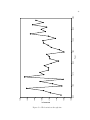
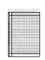
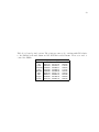
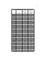
COMPARISON OF GEODETIC AND GLACIOLOGICAL MASS
BALANCE ON GULKANA GLACIER, ALASKA
By
Leif H. Cox
RECOMMENDED:
Advisory Committee Chair
Chair, Department of Geology and Geophysics
APPROVED:
Dean, College of Science, Engineering and Mathematics
Dean of the Graduate School
Date
COMPARISON OF GEODETIC AND GLACIOLOGICAL
MASS BALANCE ON GULKANA GLACIER, ALASKA
A
THESIS
Presented to the Faculty
of the University of Alaska Fairbanks
in Partial Fulfillment of the Requirements
for the Degree of
MASTERS OF SCIENCE
By
Leif H. Cox, B.S.
Fairbanks, Alaska
December 2002
iii
Abstract
The net mass balance on Gulkana Glacier has been measured since 1966 by the glaciological method, in which seasonal balances are measured at three index sites and extrapolated
over large areas of the glacier. Systematic errors accumulate through time in this method;
therefore the geodetic balance, in which errors are independent of time, was calculated for
comparison to and possible calibration of the glaciological method. Digital elevation models
(DEMs) of the glacier in 1974, 1993, and 1999 were prepared and geodetic balances computed, giving -6.0±0.5 m of water equivalent (weq) from 1974 to 1993 and -11.8±0.5 m weq
from 1974 to 1999. These are to be compared to the glaciological balances over the same intervals, which were -5.8±0.9 m weq and -11.2±1.0 m weq, respectively; both balances show a
tripling in thinning rate in the 1990s. These cumulative balances differ by less than 6%. For
this, the glaciological method on Gulkana Glacier must be largely free of systematic errors
and use a changing area altitude distribution. Relatively good contrast in the accumulation
area of the glacier increased accuracy in the geodetic method.
iv
Contents
Signature Page . . . . . . . . . . . . . . . . . . . . . . . . . . . . . . . . . . . . .
i
Title Page . . . . . . . . . . . . . . . . . . . . . . . . . . . . . . . . . . . . . . . .
ii
Abstract . . . . . . . . . . . . . . . . . . . . . . . . . . . . . . . . . . . . . . . . .
iii
Contents . . . . . . . . . . . . . . . . . . . . . . . . . . . . . . . . . . . . . . . . .
iv
List of Figures . . . . . . . . . . . . . . . . . . . . . . . . . . . . . . . . . . . . .
vi
List of Tables . . . . . . . . . . . . . . . . . . . . . . . . . . . . . . . . . . . . . .
vii
List of Appendices . . . . . . . . . . . . . . . . . . . . . . . . . . . . . . . . . . .
viii
Preface . . . . . . . . . . . . . . . . . . . . . . . . . . . . . . . . . . . . . . . . .
ix
1 Introduction
1
2 Methods and Results
5
2.1
2.2
Geodetic Balance . . . . . . . . . . . . . . . . . . . . . . . . . . . . . . . . .
5
2.1.1
DEM Creation . . . . . . . . . . . . . . . . . . . . . . . . . . . . . .
5
2.1.2
Corrections . . . . . . . . . . . . . . . . . . . . . . . . . . . . . . . .
7
2.1.3
Surface Elevation Change . . . . . . . . . . . . . . . . . . . . . . . .
9
2.1.4
Errors . . . . . . . . . . . . . . . . . . . . . . . . . . . . . . . . . . .
11
Glaciological Balance . . . . . . . . . . . . . . . . . . . . . . . . . . . . . . .
13
3 Discussion
15
3.1
Glaciological Method Accuracy . . . . . . . . . . . . . . . . . . . . . . . . .
15
3.2
Climate and Glacier Response . . . . . . . . . . . . . . . . . . . . . . . . . .
17
4 Conclusions
18
v
A Supplement to the Apex Manual
20
A.1 Before You Start . . . . . . . . . . . . . . . . . . . . . . . . . . . . . . . . .
20
A.2 Terms . . . . . . . . . . . . . . . . . . . . . . . . . . . . . . . . . . . . . . .
21
A.3 Scanning . . . . . . . . . . . . . . . . . . . . . . . . . . . . . . . . . . . . . .
21
A.4 Project Creation . . . . . . . . . . . . . . . . . . . . . . . . . . . . . . . . .
23
A.5 Camera Calibration
. . . . . . . . . . . . . . . . . . . . . . . . . . . . . . .
23
A.6 Importing . . . . . . . . . . . . . . . . . . . . . . . . . . . . . . . . . . . . .
23
A.7 Minification . . . . . . . . . . . . . . . . . . . . . . . . . . . . . . . . . . . .
24
A.8 Interior Orientation
. . . . . . . . . . . . . . . . . . . . . . . . . . . . . . .
24
A.9 Triangulation . . . . . . . . . . . . . . . . . . . . . . . . . . . . . . . . . . .
25
A.10 Automatic Extraction . . . . . . . . . . . . . . . . . . . . . . . . . . . . . .
27
A.11 Quality Control and Manual Editing . . . . . . . . . . . . . . . . . . . . . .
28
A.12 DTM Merge . . . . . . . . . . . . . . . . . . . . . . . . . . . . . . . . . . . .
28
A.13 Exporting DTMs . . . . . . . . . . . . . . . . . . . . . . . . . . . . . . . . .
28
B Camera Calibrations
30
C Archived Data
34
Bibliography
41
CD of Archived Data
Back Pocket
vi
List of Figures
1.1
Location Map . . . . . . . . . . . . . . . . . . . . . . . . . . . . . . . . . . .
3
1.2
Index Site, Weather Station, and Control Point Locations . . . . . . . . . .
4
2.1
Ablation Corrections . . . . . . . . . . . . . . . . . . . . . . . . . . . . . . .
8
2.2
Total Emergence as a Function of Elevation . . . . . . . . . . . . . . . . . .
9
2.3
Suface Elevation Change in Meters of Water Equivalent . . . . . . . . . . .
10
2.4
Glaciological Balances . . . . . . . . . . . . . . . . . . . . . . . . . . . . . .
14
3.1
Comparison of Cumulative Glaciological and Geodetic Mass Balances . . .
16
C.1 Laser Altimetry Comparison
. . . . . . . . . . . . . . . . . . . . . . . . . .
35
C.2 ELA Variations Through Time . . . . . . . . . . . . . . . . . . . . . . . . .
36
vii
List of Tables
2.1
Data Collected on Gulkana Glacier . . . . . . . . . . . . . . . . . . . . . . .
6
2.2
Seasonal Correction Interval . . . . . . . . . . . . . . . . . . . . . . . . . . .
7
2.3
Cumulative Geodetic and Glaciological Balances . . . . . . . . . . . . . . .
11
2.4
DEM Accuracy . . . . . . . . . . . . . . . . . . . . . . . . . . . . . . . . . .
11
A.1 Strip Data Dialogue . . . . . . . . . . . . . . . . . . . . . . . . . . . . . . .
25
B.1 1974 Aerial Camera Data . . . . . . . . . . . . . . . . . . . . . . . . . . . .
31
B.2 1993 Aerial Camera Data . . . . . . . . . . . . . . . . . . . . . . . . . . . .
32
B.3 1999 Aerial Camera Data . . . . . . . . . . . . . . . . . . . . . . . . . . . .
33
C.1 Cumulative and Net Balance at Index Sites . . . . . . . . . . . . . . . . . .
37
C.2 Area Altitude Distribution . . . . . . . . . . . . . . . . . . . . . . . . . . . .
38
C.3 Control Point Locations . . . . . . . . . . . . . . . . . . . . . . . . . . . . .
39
C.4 Conventional and Reference Surface Cumulative Balances . . . . . . . . . .
40
ix
Preface
This main body of this thesis has been prepared for submission to the Journal of Glaciology.
Rod March will be the second author on the paper. All of the glaciological data was either
prepared by him or based measurements made directly by him or others in the USGS. Keith
Echelmeyer and Will Harrison also spent many hours editing the paper many and helped
immensely with ideas for the scientific process, but declined to be listed as authors.
Appendices are included in the thesis that contain important information which did not
have a place in the paper. The first appendix is a sample work flow for creating digital
elevation models (DEMs) using PCI Geomatics Apex Software. Much of the time spent
working on the thesis was devoted to learning the software and creating a viable work flow
preparing DEMs for differencing. Other operators will benefit from following this appendix.
Also included is a CD so people working with this data will not have to reenter it by hand.
All of the data on the CD is also shown in appendices because it is unknown how long the
data format on the CD will be compatible with typical computers, or even how long CDs
will be used.
Will Harrison contributed a great amount to this thesis and had many ideas to improve
it. I learned from him that “it’s the systematic errors that will kill you”, and many other
things not fit for a thesis. He works too hard for a man who is ‘retired’, but his help
was greatly appreciated. Rod March had much patience helping me to find archived data
and helping with my computer when it would ‘crater’ every week or so. Roman Motyka
also read through the manuscript several times and suggested ways to improve it. Martin
Truffer had the bad luck to be the only professor consistently around, so he took the brunt
of my questioning during the writing, and also read the thesis numerous times. I would
like to thank Keith Echelmeyer for the time he put in to help me, in spite of his adverse
situation. During my time at UAF I learned an incredible amount about glaciers and
climbing from him; he also tried to beat geodynamics into me, and I think some of it stuck.
More importantly, he taught me about being persistent and careful in my work, and even
more about life in general.
Anthony Arendt contributed so much to this paper, especially in the initial stages, that
I was worried he might claim first authorship. Luckily, he already has an M. S. and claims
x
to not need another. Many of the other members of the lab, both students and faculty, read
a version of the thesis at least once, if not many times: Carl Benson, Adam Bucki, Dan
Elsberg, and Sandra Zirnheld. Thank you. I didn’t give By Valentine a change to read the
manuscript, but I didn’t want to ruin her perpetual cheerfulness. I also did not give Craig
Lingle a change to read it, but if it wasn’t for him I might never have become comfortable
with the kinematic surface boundary equation.
My wife, Trilby Cox, provided most of the support and funding for the non-work parts
of my tenure as a masters student. Thank you so much, especially for your support the last
two months of thesis writing, which we both thought might never end. I would also like to
thank my parents (both sets) and my little sister, Heidi, for late night e-mails and other
sources of encouragement.
This project was funded by the United States Geological Survey. Many thanks to Dennis
Trabant and Rod March for securing funding, and anyone else in the USGS who helped.
1
Chapter 1
Introduction
Glacier-wide net mass balance is the net gain or loss of mass over an entire glacier during a
given balance year; summing the net balance over a series of years results in a cumulative
balance. Regional trends in cumulative mass balance are indicators of climate variability
[Oerlemans and Fortuin, 1992; Hodge et al., 1998; Dyurgerov and Meier, 2000] and can have
a large effect on sea level [Houghton et al., 2001; Arendt et al., 2002]. However, world wide
there are only 33 glaciers that have a balance record over 40 years in length [Dyurgerov and
Meier, 1997], so one or two glaciers are often used to represent hundreds of glaciers in a
region [e. g. Meier, 1984]. While region-wide extrapolations may cause inaccuracies, it has
been shown that in some areas a single glacier can represent the mass balance of a region
[Rabus and Echelmeyer, 1998]. A more fundamental problem is the accuracy of the limited
number of mass balance records used for extrapolation.
The conventional method to measure mass balance, which we refer to as the glaciological
method, relies on balance measurements made at a number of discrete points. These are
then extrapolated over the glacier, usually based on the area-altitude distribution (AAD)
[Østrem and Brugman, 1991]. Accumulation of errors can be problematic in this method.
We are concerned primarily with systematic errors because they increase linearly with the
√
the number of years (N ) in the record, whereas random errors increase as N . It is
thus important to check whether the errors in the glaciological method are predominately
random, or if a large systematic component is present in the given balance record.
An independent method used to check and possibly calibrate the cumulative glaciological
2
balance is the geodetic method [Fountain et al., 1997]. In this method, maps of a glacier or
their digital equivalent, digital elevation models (DEMs), are created using photogrammetry
at intervals of a few years to a few decades. Differencing these DEMs, after applying
corrections for density and other factors, gives the glacier-wide cumulative balance for the
different time intervals. This method accounts for all spatial variability in balance, assuming
the DEMs are accurate everywhere, and references a stable geographic datum.
These two methods attempt to measure the same quantity, the glacier-wide balance, but
the results differ because of errors inherent in each method. Previous studies comparing
the results of the two methods have found systematic errors in the glaciological method and
map errors in the geodetic method. Errors in the glaciological balance have resulted from
poles sinking into the snowpack, incorrectly defined previous seasonal surfaces, and/or unaccounted for internal accumulation [Krimmel, 1999; Haakensen, 1986; Conway et al., 1999].
These errors will be summed over the glacier and combined with cross-glacier variations in
balance from surface irregularities, avalanches, wind deposits or scours, and topographic
shading [Fountain and Vecchia, 1999; Krimmel, 1999]. Such errors can accumulate systematically over time, which has been shown even to cause the glaciological balance to have
the opposite sign of the geodetic balance [Conway et al., 1999]. Errors associated with the
geodetic method are primarily due to poor photogrammetric contrast in high accumulation
areas and poor DEM registration, which in extreme cases can cause the balance to vary by
several times the accepted value [Østrem and Haakensen, 1999; Andreassen, 1999]. These
errors do not accumulate over time, making the cumulative geodetic balance more accurate
than the cumulative glaciological balance over time scales longer than a few years. The
geodetic method can thus be used to calibrate the glaciological cumulative balance [Elsberg
et al., 2001].
The mass balance record is especially important on Gulkana Glacier because it has one
of the longest mass balance records in the United States (1966-present). It is one of three
index glaciers chosen for long term balance monitoring by the United States Geological
Survey (USGS) and is the only one of these index glaciers in a continental climate zone.
It is often used for studies in glacier-climate interaction and sea level change [Letréguilly
and Reynaud, 1989; Trabant et al., 1998; Dyurgerov and Meier, 1997]. The accuracy of
the glaciological balance on Gulkana Glacier has not been independently verified. Here we
3
determine the geodetic balance over two intervals for comparison to and possible calibration
of the glaciological record.
Alaska
Fairbanks
Gulkana Glacier
Anchorage
Kilometers
0
250
500
1,000
Figure 1.1. Location map.
Gulkana Glacier is located in the eastern Alaska Range (63o 16’ N, 145o 25’ W) (Figure 1.1).
It has three accumulation cirques, facing approximately south-east, south, and west, with
the maximum elevation of 2450 m in the south-east facing cirque known as the Minya Basin.
Ice from the three accumulation areas merges below the average equilibrium line altitude
(ELA) of 1780 m and flows south to the terminus at 1200 m above sea level [March, 1998].
The terminus has retreated 3 km since its Little Ice Age maximum at the turn of the 20th
century [Péwé and Mayo, 1983] and about 300 m since 1974. Glacier area has decreased
from 18.4 km2 in 1974 to 17.1 km2 in 1999. The average balance gradient is 0.5 m a−1 /100 m.
Air temperature and precipitation have been measured since 1967 at a weather station located on a moraine east of the lower glacier; the record is 93% complete [Kennedy et al.,
1997].
Presently there are three index sites on the glacier (labeled as A, B, and D as shown in
Figure 1.2) at which surface motion and mass balance have been measured by the USGS
since the mid 1970’s [March, 1998]. Three laser altimetry elevation profiles were flown in
1993, 1995 and 1999, and the glacier elevation profile was optically surveyed in 1993.
4
Figure 1.2. Index site, weather station, and control point locations.
5
Chapter 2
Methods and Results
2.1
Geodetic Balance
Geodetic balances for Gulkana Glacier were calculated using aerial photography from 1974,
1993, and 1999 (Table 2.1). (See Appendix B for camera calibrations and photography
credits.) AeroMap US (Anchorage, Alaska) had previously created a high quality DEM
from the 1993 photographs, but due to problems transferring control points to the 1974
and 1999 images and for increased relative accuracy, we made another DEM from the 1993
photographs. Photos taken in 1974 are high quality, but lack coverage in the upper Minya
Basin, as will be discussed below.
2.1.1
DEM Creation
We generated three DEMs of Gulkana Glacier from the aerial photographs using a digital
photogrammetry system (PCI Geomatics Apex). The digital process is very similar to
analytical photogrammetry except that the photographs are scanned to create a digital
image, the extraction of elevations is semi-automated, and a 3-D viewing system is used to
edit the DEMs. Scan resolution limits accuracy, with a horizontal accuracy equal to about
1 to 2 times the ground pixel size (the ground dimension represented by one pixel) and a
vertical accuracy of 0.5 to 3 times the ground pixel size [PCI, 2000].
Two types of control are used to orient images: control points, which orient the images
to absolute ground coordinates, and tie points, which align the images to each other. In
6
Table 2.1. Data collected on Gulkana Glacier. This data was used to prepare DEMs and
assess DEM accuracy.
Data
Date
Collected
Number of
Photo
Focal
Scan
Ground
Photographs/
Scale
Length
Res
Pixel
Points
Aerial
(mm)
(µm)
Size (m)
9/7/1974
4
1:22000
151.293
10
0.22
7/11/1993
8
1:36000
153.211
10
0.37
Photography
Aerial
Remarks
Missing Minya
Basin, Monochrome
Excellent Quality,
Photography
Aerial
Color
8/18/1999
9
Laser Profile
6/12/1993
≈ 10, 000
Laser Profile
6/3/2000
≈ 10, 000
Optical Profile
8/1/1993
56
Photography
1:24000
151.830
7
0.17
Poor contrast in upper
basins, Monochrome
1992, ten control points were surveyed to about ±0.1 m using the Global Positioning System
(GPS) (Figure 1.1); these were marked on the ground with 10 m x 10 m white crosses that
were easily identified on the images acquired the following year. Images from 1974 and 1999
lacked these or any other marked control points; they were oriented using obvious features
such as rock outcrops and mountain peaks. When these features are selected in multiple
images they become the tie points, which allow the uncontrolled images to be aligned with
controlled images. A total of 170 tie points on bedrock were used as coincident image points
for this relative control.
After the images were properly controlled, an algorithm using image correlation automatically extracted DEMs on 5 m co-registered grids, which we found was optimal for image
correlation. To facilitate manual editing, which was only needed on an estimated 10% of
the glacier, the grids were resampled glacier-wide to a 25 m spacing. Andreassen [1999] has
demonstrated this is a suitable grid spacing for geodetic balance calculation.
Manual editing was needed in areas of low contrast, such as the upper Minya Basin
where bright snowfields display few features to be correlated. Manual editing is difficult in
these areas, and care must be taken to not “float” the grid points in bright areas to a higher
elevation than dark areas for lack of other information. Grids were not extracted from
the 1999 Minya Basin because of poor contrast; instead, a triangulated irregular network
(TIN) was used. Unlike the grid method, in which the software picks a point at every
7
grid node regardless of accuracy, the TIN method effectively only extracts points with an
image correlation coefficient greater than a specific value. This eliminates the process of
the operator manually editing thousands of inaccurate points, although some accuracy is
lost because the point density may be reduced as much as an estimated ten times in very
poor contrast areas.
2.1.2
Corrections
Before differencing, there are three corrections that we need to apply to each DEM to get
geodetic balances that can be directly compared to the glaciological balances: ablation,
emergence, and density. Ablation and emergence corrections were applied because the date
of photography did not coincide with the end of the ablation season, which is when the
glaciological balance is measured (see Table 2.2). We refer to these as seasonal corrections.
Density corrections convert snow or ice volume to water equivalent volume change.
Table 2.2. Seasonal Correction Interval. The duration of seasonal correction is shown with
the glacier wide ablation correction. Emergence corrections were applied over the same
interval.
Photography
End of
Interval
Glacier-Wide
Date
Ablation Season
(days)
Ablation Correction (m weq)
9/8/1974
9/20/1974
12
-0.2
7/11/1993
9/8/1993
59
-1.8
8/18/1999
9/26/1999
39
-0.3
The ablation corrections were done following the concepts of Reeh [1991] using the simple
degree day model of Arendt [1997]. Measured summer precipitation, temperature, and the
DEM for each year were input into the model. The model was then tuned by varying
temperature lapse rates and degree day factors to force the modeled summer balance to
match the summer balance measured at each index site. Finally, the ablation in meters of
water equivalent from the date of photography to the end of the balance year was calculated
as a function of elevation (Figure 2.1). The 1993 corrections are relatively large, especially
at low elevations, because of the long time interval and the fact that this period extended
over the most intensive part of the ablation season. Internal ablation and accumulation are
assumed to be negligible over the intervals.
Ablation Correction (m weq)
8
0.00
-1.00
-2.00
1974
1993
1999
-3.00
-4.00
-5.00
1150
1650
Elevation (m)
2150
Figure 2.1. Ablation corrections. The corrections were tuned to match measured seasonal
ablation at index sites represented by vertical dotted lines.
We also corrected each DEM for total emergence from the photo date to the end of the
ablation season over the interval shown in Table 2.2. Any change in the surface elevation of
the glacier at a point not due to ablation is due to the emergence velocity; it is the vertical
component of velocity corrected for the downstream movement of ice [Paterson, 1994]. We
define the total emergence to be the cumulative surface elevation change from emergence
velocity over the interval. It should be noted emergence does not affect glacier-wide balance
because it is merely a redistribution of mass along the entire glacier. Nevertheless, we
corrected the DEMs for emergence velocity for two reasons: 1) to more accurately compare
individual DEM points with optical and laser profiles (see section 2.1.4), and 2) to more
accurately represent the thinning at specific areas at the end of the ablation season. A
curve was fit through the total emergence measured over the interval at the index sites and
adjusted to the shape of the extended mass balance curve (see section 2.2). Flow was not
measured in 1974, so the average emergence from 16 years data at each index site was used.
The shape of the curve from 1993 differs from the others because the measured emergence
at the mid-glacier site (B) was greater than the index site low in the ablation area (Fig.
2.2).
Thickness changes of ice or snow were converted to water equivalent based on the density
of the material lost or gained. The small shift in the ELA during the measurement period
(Figure C.2) and the relatively small balance gradient make the assumption of Sorge’s Law
9
Total Emergence (m)
0.5
0.3
0.1
1974
1993
1999
-0.1
-0.3
-0.5
1150
1650
2150
Elevation (m)
Figure 2.2. Total emergence as a function of elevation. This was measured over the correction intervals at the index sites represented by vertical dotted lines.
plausible on Gulkana Glacier. This law states that the density structure remains constant
in an unchanging climate [Bader, 1954], allowing us to assume that the change in volume
is related directly to water equivalent volume by the density of ice (900 kg m−3 , Paterson
[1994]).
2.1.3
Surface Elevation Change
Surface elevation change was calculated by differencing two registered DEMs over the glacier
surface. Where a surface change varied by more than 5 m from adjacent areas, the point was
remeasured in the original DEM. Points where elevations could not be extracted accurately
due to poor contrast were removed and the elevation change interpolated from adjacent
locations. The intervals 1974 to 1993 and 1993 to 1999 were differenced, and the geodetic
balance from 1974 to 1999 was simply the sum of the two intervals. Any errors in the 1993
DEM will be removed in this summation, so no inaccuracy was included.
The upper 2.7 km2 of the Minya Basin did not contain registered grids to subtract because the 1974 photography did not cover this area and the 1999 photographs had low
contrast. Thus, the 1974 to 1993 surface elevation change in the Minya Basin was extrapolated from surrounding regions. It was assumed to have no surface change because 1) the
high areas of the glacier for which coverage existed showed no change over the interval and
10
2) the surface change of the lower Minya Basin trended to zero at the edge of coverage. The
1999 TIN in the upper Minya Basin was subtracted from coincident 1993 grid points, and
the surface change was interpolated between measured points.
When all the corrections were applied, the elevation changes shown in Figure 2.3 were
obtained. The cumulative geodetic balance then is equal to the glacier-wide average surface
elevation change integrated over Figure 2.3. For 1974 to 1993, the geodetic balance was
-6.0 ±0.5 m weq and it was -5.8 ± m weq from 1993 to 1999. Addition of these two balances
leads to a strongly negative balance over the entire interval from 1974 to 1999, as shown in
Table 2.3.
Figure 2.3. Surface elevation change in meters of water equivalent. The maps are the two
intervals 1974-1993 (a) and 1993-1999 (b).
11
Table 2.3. Cumulative geodetic and glaciological balances.
Interval
2.1.4
Geodetic
Glaciological
Balance (m weq)
Balance (m weq)
1974-1993
-6.0 ±0.5
-5.8 ±0.9
1974-1999
-11.8 ±0.5
-11.2 ±1.0
Errors
Errors in the geodetic balance can result from seasonal corrections, image control, and
elevation extraction—especially in the low contrast accumulation areas. Both absolute
control of the DEMs to the map datum and relative control between different DEMs account
for errors in image control. These are addressed separately in the following three paragraphs.
Fifty six points were surveyed on the glacier in 1993 to an accuracy of ±0.1 m (Table 2.1).
These points were well distributed over the glacier with one profile up each of the main
branches and several longitudinal profiles. Each of the profiles was subjected to the same
seasonal corrections as the DEMs. Comparison of DEM elevations to the optically surveyed
points shows that the DEM is systematically 0.74 m weq too low (Table 2.4). There appears
to be no systematic trend to the offset with elevation, although the standard deviation is
greater for points in the accumulation area. The systematic difference was greater than
expected, and we cannot find a satisfactory explanation for it.
Table 2.4. DEM accuracy. The standard deviation about the mean is greater over the
bedrock than ice, and the relative error among DEMs is small. The standard deviation
about the mean shows the accuracy of an individual measurement; this demonstrates how
accurate a single point can be extracted. The standard deviation of the mean is how well
the mean offset is known.
Data
Mean
Standard
Standard
Remarks
Offset
Deviation about
Deviation of
(m weq)
the Mean (m weq)
the Mean (m weq)
Bedrock 1993-1974
-0.20
4.70
0.22
Relative Error
Bedrock 1999-1993
-0.12
5.20
0.15
Relative Error
Optical Survey - 1993 DEM
0.74
1.34
0.20
Absolute Error
2000 Profile-1999 DEM
0.21
1.87
0.15
Absolute Error
1993 Profile-1993 DEM
0.49
1.67
0.15
Absolute Error
Airborne laser altimetry profiles flown in 1993 and 2000 were measured to an accuracy
12
of about ±0.3 m [Echelmeyer et al., 1996]. These profiles cover the centerline of the main
branches in an almost continuous line down the glacier [Sapiano et al., 1998]. The 1993
and 2000 laser altimetry profiles show the 1993 DEM to be 0.55 m weq low and 0.23 m weq
low, respectively (Figure C.1). These also show no trends in the difference indicating the
DEMs are not sloping relative to the datum. The mean offset is probably due to the long
duration over which seasonal corrections were calculated. The important results of the
profile comparisons are that the absolute accuracy of the 1993 and 1999 DEMs is less than
1 m, and that the accuracy of elevations extracted in the accumulation area are satisfactory.
We did not use these independent profiles as an indication of error among the DEMs. We
considered relative error to be a much better indication of this.
The relative accuracies of the DEMs were checked by subtracting two DEMs over
bedrock. The relative error among DEMs is more important than the absolute error of
the DEMs when calculating geodetic mass balance because it indicates the total systematic
error in the geodetic balance. We note that there are several factors which may make the
point measurements over bedrock less accurate than those over ice. The first problem is
that the photographs were scanned to optimize contrast over the ice and snow areas making
the bedrock dark (and often black) in many areas. Second, bedrock areas were not manually edited as carefully as the glacier areas. Third, except for a few locations, the only
snow free areas near the upper glacier are nearly vertical causing large elevation errors from
small horizontal registration errors. The increased standard deviation about the mean of
the DEM over bedrock compared to measurements on the glacier illustrates these problems.
In spite of the difficulties, the bedrock differencing gave encouraging results, with less than
0.3 m error among DEMs.
Our error budget for the geodetic balance includes elevation extraction, emergence corrections, density, ablation corrections, and relative orientation. Elsberg et al. [2001] showed
that geodetic balances on South Cascade Glacier would have changed by less than 5.5%
if firn is lost in the mid-elevations of the glacier instead of ice. Gulkana Glacier has experienced much less change than South Cascade Glacier over the measurement periods, so
any error associated with assuming Sorge’s Law will be at most a few percent. Seasonal
corrections, especially in 1993, and relative orientation of the DEMs are the largest errors.
These are both estimated at 0.3 m weq. Based on these estimates, we take as a conservative
13
estimate of the error in the geodetic balance over each interval to be ±0.5 m weq.
2.2
Glaciological Balance
The USGS has used the glaciological method to determine the net mass balance on Gulkana
Glacier every year since 1966. In this method, the end of the balance year is defined as
the date of the yearly glacier-wide minimum balance. They maintained an extended stake
network of up to 30 mass balance stakes until the mid-1970s, when the stake network was
reduced to three index sites (see Figure 1.2) and measurements were expanded to include ice
motion and surface elevation at these sites [March, 1998]. Since 1974, the balance has been
calculated using data from these three index sites . The highest index site (D) is generally
just above the ELA, but the ELA has been above site D three times. The seasonal balance is
measured in an area 25-75 m around each pole, in an effort to reduce errors from individual
snow depth soundings and small scale surface irregularities [Trabant and March, 1999].
To calculate the glacier-wide balance from the index site measurements, the glacier is
divided into three elevation bins each centered at elevations halfway between the elevations
of sites A and B, and sites B and D. The elevation bins are updated each year for the
variations in index site altitude, but not for changes in glacier area. The map area of each
elevation bin is divided by the total area of the glacier to obtain an area weighting factor.
This is equivalent to using an area altitude distribution. The weighting factor is multiplied
by the balance at each site and the results are summed to determine the glacier-wide surface
elevation change. Estimated internal ablation from geothermal heat, ice motion, and water
flowing through and under the glacier is added to the surface balance to find a glacier-wide
net balance [March, 1998].
The 1967 area altitude distribution (AAD) was used to calculate the area weighting
factors from 1966 to 1993. A new AAD was recalculated in 1993 by the USGS, and all
subsequent balances have used the 1993 AAD. For consistency, all prior balances starting
with 1966 were recalculated by the USGS with the 1993 AAD. All previously published
balance measurements are therefore referenced to a fixed AAD, which effectively yields the
‘reference surface’ balance of Elsberg et al. [2001]. This balance is the appropriate variable to
compare to climate, but it does not represent the true volume change and cannot be directly
14
compared to the geodetic balance. For this comparison, we have established time-variable
AADs by calculating the area altitude distribution from DEMs of 1974, 1993, and 1999.
These were then interpolated for the intervening years (see Table C.2). The glaciological
balances presented in this paper are ‘conventional balances’ and were calculated using these
time-variable AADs. Again, there is a trend toward more negative balances in the 1990s as
shown in Table 2.3 and Figure 2.4. The comparison between the conventional and reference
surface balances are shown in Figure 3.1 and Table C.4.
The published error for the glaciological balance on Gulkana Glacier is 0.20 m a−1
[March, 1998]. To verify this, the USGS calculated balances for 1966 and 1967 using both
the expanded pole network and the three index sites. The expanded pole network reduces
much of the balance interpolation with elevation, and the difference between the two methods was within ±0.2 m a−1 . However, the expanded stake network result was not used for
calibration, nor does the difference indicate whether the error is systematic or random.
Figure 2.4. Glaciological balances: (a) net balance and (b) cumulative balance. The cumulative balance is bounded by random (dark gray) and systematic (light gray) errors of
0.2 m weq a−1 .
15
Chapter 3
Discussion
3.1
Glaciological Method Accuracy
The comparison between geodetic and cumulative glaciological balances is shown in Figure 3.1 and Table 2.3. The comparison is excellent, with the geodetic balance within the
estimated error bars of the glaciological balance. This implies that the glaciological balance method on this glacier does not have large systematic errors that could arise from
several sources including sinking poles, erroneous snow depths, missing internal ablation
and accumulation, and an invalid area extrapolation. The USGS includes an estimated
0.05 m weq a−1 internal ablation in the net balance. Systematically ignoring this small factor would have decreased the cumulative glaciological balance by about 10%.
On Ålfotbreen Glacier, Østrem and Haakensen [1999] placed plywood at the base of mass
balance poles and observed poles forced through the plywood due to snow compaction. The
USGS circumvented this problem by laying plywood or sawdust on the summer surface to
unambiguously locate it the following spring by drilling or coring [Trabant and March, 1999].
In addition, single point measurements are not necessarily representative of the immediate
area; deviations of 0.23 m weq in one year have been observed on three stakes less than
5 m apart [Braithwaite and Olesen, 1989]. Errors from these variations can sometimes be
eliminated by sampling the balance in an area tens of meters around each index site, which
the USGS does in both the ablation and accumulation season [Trabant and March, 1999].
Even with perfect point balance measurements, three poles have not typically been
16
Figure 3.1. Comparison of cumulative glaciological and geodetic mass balances. The geodetic is shown to be within the random error (gray) of the glaciological balance. The 1967
reference surface balance is shown to differ from the conventional balance.
found sufficient to accurately determine the mass balance on glaciers the size of Gulkana;
a minimum of 5 to 10 poles is recommended [Østrem and Brugman, 1991; Fountain et al.,
1997]. Krimmel [1999] found differences of 30% on the relatively small (≈2 km2 ) South
Cascade Glacier, Washington, in a 27 year balance record; this was in part due to area
extrapolation using between 1 and 20 poles. Our results seem to indicate that three poles
are adequate to represent the balance on Gulkana Glacier. This could be due to the balance
curve being well correlated across the glacier and with elevation, and the pole locations
accurately represent the areas intended. But it is surprising that one index site located
generally just above the ELA represents the entire accumulation area.
The reference 1967 reference surface balance differs from the actual mass change as
shown in Figure 3.1. Reference surface balances are valuable, especially when relating balance to climate [Elsberg et al., 2001], but must be stated as such when published because
they are not the actual mass change of a glacier and cannot be directly compared to the
geodetic balance and hydrologic outflow. For accurate comparisons, the conventional glaciological balance as shown in Figure 3.1 and Table 2.3 is needed. The geodetic balance can
be used to correct the reference surface balance to a conventional balance using a one or
two parameter fit as outlined by Elsberg et al. [2001].
17
3.2
Climate and Glacier Response
The geodetic balances correspond to an average annual thinning rate of 0.31 m a−1 from
1974 to 1993 and 0.96 m a−1 from 1993 to 1999. This accelerated thinning rate in the 1990s
has been observed nearly everywhere in Alaska [Arendt et al., 2002]. The more continuous
cumulative glaciological balance record shows these trends as well (Figure 2.4).
The total thinning is much greater near the terminus over the first period (Figure 2.3).
From 1974 to 1993, we found a maximum thinning of 60 m weq, compared to the second
interval with a maximum of 40 m weq. However, during the first interval there is little
change in the accumulation area, while in the second interval there was 4 m weq thinning
in the accumulation area. This trend has been witnessed in most of Alaska [Arendt et al.,
2002]. Lower net accumulation rates in the accumulation area, accompanied by a general
glacier velocity decrease, would lead to such patterns of change.
18
Chapter 4
Conclusions
The agreement of the two mass balance methods on Gulkana Glacier is encouraging. It
supports the use of the limited number of index sites for determining the net glaciological balance if sufficient care is make in the required measurements and corrections. The
glaciological mass balance of Gulkana Glacier can be accurately represented by three index
sites with only one accumulation area site located just above the average ELA. This also
demonstrates that the balance in a small radius can accurately describe the balance in an
elevation band, and the extrapolation with elevation and area has no large systematic errors
on this glacier.
This does not necessarily apply to other glaciers or even to future measurements of
Gulkana Glacier. Every glaciological mass balance record needs to be regularly calibrated
with the geodetic method. The relatively small error of the carefully measured glaciological
balances makes them ideal for annual measurements and the time independent nature of
the geodetic method makes it ideal for long term (several years to decades) measurements.
Many glaciers have featureless accumulation areas, this can account for large errors in
the geodetic balances. The accumulation area on Gulkana Glacier is broken up into several
small cirques with numerous nunataks and crevasses that aid stereo viewing. The snow
line was also anomalously high during each year of photography, providing better contrast
at high elevations. There was excellent relative control due to numerous tie points with
concurrently made DEMs. Ablation corrections were calculated using a temporally and
spatially tuned model.
19
We recommend several steps that can produce more accurate comparisons and possible
calibrations of the glaciological method. The photography should be taken as close to
the end of the balance year as possible; this will decrease the amount of error due to
seasonal corrections and decrease the amount of snow at higher elevations, aiding stereo
perception. Second, if possible, mass balance poles should be surveyed near the time of
aerial photography so the balance between photography and the end of the ablation season
can be determined. It is useful to have an independent profile of the glacier surface to check
the DEM. A reference surface balance (which is at present published by the USGS) cannot
be directly compared to actual mass change. The conventional balance, which includes
changes in the total glacier area and AAD, is needed for an accurate comparison.
20
Appendix A
Supplement to the Apex Manual
A.1
Before You Start
Apex is a digital photogrammetry system written by PCI Geomatics [PCI, 2000]. The
published manual for the software lacks an organized work flow, and some directions are
ambiguous. This appendix is designed to go along with the manual, outlining the steps
necessary to create accurate DEMs, and providing more detail when needed. The following
will be enough to get one started and reproduce the DEMs used for this thesis. This is by
no means a comprehensive manual. The scanning section should be read prior to scanning,
but the rest of the sections will probably make little sense without the program running in
front of you.
Apex is very finicky, it often will corrupt files and then save them upon exiting. I
recommend backing up the entire data directory every time much progress has been made
by copying the entire file into anther directory using windows explorer. Commands are also
often grayed, sometimes because a window was closed with the x instead of file→ exit, or
sometimes it just seems to happen. This is fixed by exiting and reopening the program.
Apex saves all progress automatically on exiting, so if an error is made before exiting, the
data will have to be reloaded from a backed up version. There are also shortcut keys for
virtually every Apex command; familiarization with these will speed repetitive processes.
Apex is well suited to creating accurate digital terrain models (DTMs), but is not
effective for DTM analysis. Another program such as AutoCad with the Quicksurf addition
21
or ARC should be used for anything but the most basic analysis. DTM is interchangeable
with digital elevation model (DEM), as used in the paper. I used DEM in the paper because
it is more common in literature, but use DTM here because this is the terminology Apex
uses.
A.2
Terms
Minification: The largest view without interpolation is 1:1, and each larger scale allows
you to see more of the image. For each scale (e. g. 1:64) a new image is created during
minification so zooming is faster.
Interior Orientation: This process corrects an image for lens distortion.
Exterior Orientation/Triangulation: This process orients an image either relative to
other images or to true ground coordinates.
Console Monitor: The monitor which displays menus and is not in 3D.
Extraction Monitor: The monitor which displays in 3D.
Photograph: The picture taken by aerial photography.
Image: The digital picture after scanning.
Fiducial: Crosses or dots on aerial photographs which are used to correct for lens distortion.
A.3
Scanning
Three things are important in scanning: the resolution—typically measured in pixels per
inch (ppi), the bit depth (10 bit or 8 bit), and the image orientation. The scan resolution
directly affects the accuracy of the software. The horizontal accuracy of the software is
1-2 times the ground pixel size (the width in ground space of one pixel) and the vertical
accuracy is 0.5 to 3 times the ground pixel size [PCI, 2000]. The ground pixel size can be
22
computed from the following formula:
PM = (
S
1
)·(
)
PPI
39.37
(A.1)
where PM is the ground pixel size in meters, S is the scale, and PPI is the scan resolution in
ppi [Slama, 1980]. The effectiveness of a higher scan resolution will decrease when the grain
of the photographs becomes visible. Less than perfect image control and lens distortion will
also decrease accuracy.
Different bit depths can be specified, with color typically scanned in 8 bit, while 10 bit
is reserved for black and white. Apex currently does not use the full 10 bits for automatic
extraction, but the images can be viewed and manually edited in 10 bits. This was tried with
the black and white photos on Gulkana Glacier and little was gained in terms of increased
contrast from 10 bit depth. The images required 4 times more memory and do not export
well, so I would recommend using 8 bit depth.
The scanning orientation does matter with Apex. The images must be either scanned
left or right as defined by the Apex manual. Left or right scan direction relates to the overlap
region of the image. If you display the images side-by-side, the overlap must either be on
the left or the right, not the top or bottom. If the photographs are scanned with incorrect
orientation, it can be corrected in Apex but is time consuming. One other consideration is,
as of this writing, Apex cannot handle images over 2 Gb.
When you transfer the scanned images to the computer, create a folder in the Apex
directory under apex_v70\usr\geoset\images called ‘MyProjectName’. You will need
room for all the images, plus room for minified images which take up again as much room
as the original images, plus about 1 Gb for other files. If there is room on the drive where
Apex is located, transfer the images to the folder you just created. If there is not room on
the local hard drive, the images can be put anywhere on the network.
Renaming the images to a standard convention will simplify the triangulation process.
Name the first image from strip one 1_1, and the second image in the same strip name
1_2, etc. A strip is a series of images taken on one flight line, and the image number is the
order the images where taken on that flight line. The numbering order of the strips does
not matter, and images can be labeled in the reverse order in which they were taken.
23
A.4
Project Creation
Open project creation with preparation→ create/edit project. Click on location→ new location; type the project name in the first column and the path to folder you created in the
second, then save it. Create the project as outline in the manual.
A.5
Camera Calibration
The camera calibration is straight forward and described well in the manual. Camera
calibrations are kept on record for a long time, so they can usually be found through the
organization that originally took the photos. Camera calibration used for this project can
be found in Appendix B.
A.6
Importing
Once the camera calibration is entered, import the images into Apex. Select preparation→
import→ image→ frame to bring up the correct window.
1. Click on the location box. If the images are stored in the
apex_v70/usr/geoset/images/MyProjectName folder, select this location. If they
are stored elsewhere, create a new location as before with a new name for the location
and the path directing the program to the image location.
2. From the file menu, select the correct camera calibration for the images.
3. Select file→ import other→ image. Browse for the image you would like to import
and select it. It should be in the folder you specified in location.
4. This will bring up the photo data window; the coordinates refer to the location of the
image corners in millimeters relative to the image center. Typically for an image with
the data strip on the left, the upper left will be x=-114, y= 114, and the lower right
will be 114, -114. This is rather unimportant as interior orientation will correct any
problems with this.
5. On the create files tab, select support only.
24
6. Go to options and deselect the auto minify option. Click start and the image should
be imported.
7. Repeat this for all images, making sure to apply the right camera calibration if using
images from different cameras, and change the location as needed.
Make sure the images have loaded properly by exiting from import and selecting in the
main window, file→ load images; select view 1 and load the images. If nothing comes up,
click move to load point in the display utility window. You will not be able to zoom out
at this point. If you see nothing check the images in any kind of image viewing software to
make sure they are readable.
A.7
Minification
Go to the main window again and select preparation→ minification. Select an image you
want to minify it but don’t click start. Open another minification window and select a
different image. Do this with all the images, then start all. They will take about 15
minutes each. When this is finished, again load the images and make sure they are visible;
this time you should be able to zoom out. Anytime you make a change to an image, you
will have to close and reopen the load image window for it to load the updated image.
A.8
Interior Orientation
Use the manual interior orientation under preparation→ interior orientation→ manual interior orientation. Whenever picking specific points on an image use the extraction monitor.
Sometimes the console monitor does not register points correctly. Locate the first two fiducials, accepting each one and then click locate all fiducials. Check the locations that were
automatically located. You can either move the point or click accept and move on. The
residual should be less than 1.0 according to the manual, but I haven’t had luck getting the
residuals below 2. Make sure you save before loading the next image.
25
Table A.1. Strip data dialogue. This is a guide for entering data in the table.
Current Image ID
1
The number of images
in the current strip
Ref Strip ID
Current strip number
Same as previous box
minus 1 (1 if current strip is 1)
Reference Image ID
1
Number of images in
strip minus 1
A.9
X(along strip)
0
0
Y(across strip)
-160
-160
(First strip enter 0)
(0)
Triangulation
This is the most difficult and time consuming part of the process. It is also the most likely
to corrupt files, so back up often. After every step, back up to a separate folder as outlined
before. Open the triangulation window by clicking preparation→ triangulation. If working
on a surface that has changed though time such as a glacier, control all the images together
using bedrock and control points to tie the images. When extracting DTMs, only use images
from the a single year.
Setup: Setup is the first step. This is where you tell the program where the images are in
relation to one another and what algorithms to use for triangulation. For the most
part, this is very straight forward if the standard naming convention was used for the
images. All of the software defaults will work well.
With the naming convention used, the first number is the strip, and the second is the
image in that strip. This window will be fairly straight forward to fill in, with the
exception of the the strip data information. When all the rest of the fields are filled
in, click the strip data button on the lower right hand of the window. This brings up
a dialog which is not well explained in the manual. The numbers to write in each box
are shown above in Table A.1.
To figure out the scan direction, use image loader to load the first two images of a
26
strip into view 1 with image 1 on the left and image 2 on the right. If the overlap
region is to left of image 1, the scan direction is left. Repeat this for all the strips.
Enter the correct scan direction for each strip. Up and Down do not work and will
corrupt you files.
In the main triangulation window, go to reset→ support file→ backup support. This
will back up your work. The data can be restored under the same menu. I have had
problems with the backup getting corrupted, so also back up the entire data directory
to another folder by cutting and pasting in windows explorer.
Exterior Initialize: Exterior initialization is the next step. Click the initialize/solve tab
at the bottom of the triangulation window and select exterior initialize. You just
backed up the support files, so click through the first message. Run the orientation.
Now save the triangulation file and exit. Open the load imagery dialog, load image
pairs (e. g. 1_1 and 1_2) one at a time, and examine the images to make sure the
overlap area is approximately correct. If it is not, go to image enhancement→ pairwise
rectify. If this doesn’t make the images line up there is an error, probably with the scan
direction. The program will let you proceed, but do not until the images are correct.
Also, do not run exterior initialize after blunder detect and solve or simultaneous
solve. This can cause file corruption.
Control Point Editor: Bring up the control point editor by clicking preparation→ control
point editor. Now select File→ Select GPF and name a new file. Enter the control
point names and coordinates, making sure to click accept before adding a new point.
Include the accuracy because it will be used in the final triangulation solution. Save
this and exit.
Interactive Point Measurement: Go back into triangulation and click on interactive
point measurement (IPM). If many of the commands are grayed out, select view 0 in
the display utility. In the IPM window, click grnd file and select the file that you just
created in the control point editor. The IPM process is fairly straight forward and
well described in the manual. Pick at least four points, control or tie, in each image,
and make sure each strip is tied together with at least four points. Save and exit after
picking points.
27
Blunder Detect and Solve: Click on initialize/solve→ blunder detect and solve. Deselect point distribution for now. This can be useful for checking the control and tie
points distribution later, but first you want to get the images initially oriented. Click
start. Clicking on edit failures will tell you which images need more tie points or if
there is a bad point. You can adjust the image parallax and other parameters to make
this less rigorous. Iteratively run this tool and interactive point editor until blunder
detect and solve is successful. If things are not going well, check the image orientations as before with the image loader. If the images are not close to their expected
relative locations, (i. e. the overlap region is not correct), you will have to reload the
backed up support files and add tie points, or correct erroneous ones.
Simultaneous Solve: After blunder detect and solve has been successful, run simultaneous solve. This will perform a least square inversion on all the images simultaneously.
Click on initialize/solve→ simultaneous solve. After hitting start, check the image
pixel residual; the manual recommends this be lower than 1 for a final solution. If the
whole solution is poor, i. e. the image residual is greater than 5, tie or control points
will have to be corrected or tie points added. If it is very high (>1000) there is an
erroneous data point or an error in setup. (Note that the window will not resize to
accumulate large numbers, so a huge value such as 1.23456789e+120 might be interpreted as 1.23456.) If the residual is very large you will need to reload the backed up
files and start again at setup. Click on display residuals. This displays all control and
tie points in ascending order of accuracy. Points with large residuals will have to be
remeasured. This can be done either from the current window or in the interactive
point editor. Keep adjusting points until an acceptable solution is reached.
A.10
Automatic Extraction
Once the images are controlled, exit triangulation and click extraction→ terrain→ automatic
DTM extraction. The setup is explained well in the manual, and the default values work
well, so I will not belabor the process here. A few hints on automatic extraction. Use
a spacing that results in approximately 10,000 points for the first extraction, which is
small enough to run quickly and large enough to give meaningful results. Check it in the
28
interactive edit which is explained below. The terrain may need to be broken up into several
different areas to be correctly extracted. Likely breaks between DTMs are large changes
in slope or brightness (e. g., from the glacier to the valley walls). You can open several
automatic extraction windows at the same time and run them overnight. I’ve found the
best spacing to be 3-5 m. Smaller spacing does not increase accuracy, and larger spacing
seems to deteriorate accuracy.
Some regions may not have enough contrast to be accurately picked by either you or
the computer, so it may be beneficial to use triangulated irregular networks (TIN). The
computer will effectively only pick points within a certain confidence interval when using
the TIN method with heavy mass point thinning selected. This eliminates trying to edit
thousands of inaccurate points in a low contrast area.
A.11
Quality Control and Manual Editing
Open Extraction→ Interactive edit and load a DTM. View each automatically extracted
grid; where large areas are inaccurate, either change the grid spacing to a smaller grid, or
break the area into more regions. You should not have to manually edit large parts of the
DEM. Rerun inaccurate regions in automatic extraction. Once all the grids are acceptable
with only small amounts of manual editing needed, use DTM merge to resample the grid
to a larger grid size. I’ve found 25 m spacing to be accurate, but not an impossible number
to manually edit; this will depend on the size of the area and the accuracy needed.
A.12
DTM Merge
Select extraction→ merge. DTM merge will resample grids to larger or smaller spacings,
change the area covered by a DTM, and combine multiple DTMs. It is explained well in
the manual.
A.13
Exporting DTMs
This is a fairly straight forward process outlined well in the manual. Use the xyz format
to export the DTMs for evaluation in another program. Because Apex puts a header on
29
the exported ascii file, you may need to open the file in a text editor and erase the heading
before using it in another program.
30
Appendix B
Camera Calibrations
31
Table B.1. 1974 Aerial Camera Data. This camera was used by Austin Post of the USGS
to photograph Gulkana Glacier in 1974. The photographs are located in the ICA collection
Geodata Center, UAF, Fairbanks, Alaska.
Camera and Lens
Camera Type
Lens Type
Camera Serial Numer
Lens Serial Number
KC-1B 67-208
475
Calibrated Focal Length (mm)
151.283
Distortion Parameters
Dc
Field Angle
Degrees
(µm)
7.5
4
15
9
22.5
2
27.5
-5
30
-6
32.5
-8
35
-9
37.5
-4
40
2
42.5
0
45
-24
Principle Points
x (mm)
Indicated principle point
(corner fiducials)
Indicated principle point
(midside fiducials)
Principle point of
autocollimation
Calibrated principle point (point
of symetry)
y (mm)
-0.005
-0.001
-0.013
0.015
Fiducial Locations
Data Strip
D
B’’
B
A
B’
C’
C
C’
A
B
C
D
B’
B’’
C’
C’’
x (mm)
-120.350
117.503
-0.011
0.010
117.409
117.681
-76.181
75.119
y (mm)
0.000
0.000
-117.804
117.591
-76.108
75.217
-117.516
-117.914
32
Table B.2. 1993 Aerial Camera Data. This camera was used by AeroMap US (Anchorage,
Alaska) to photograph Gulkana Glacier in 1993.
Camera and Lens
Camera Type
Lens Type
Camera Serial Numer
Lens Serial Number
Zeiss RMK A 15/23
Zeiss Pleogon A@
111683
112649
Calibrated Focal Length (mm)
153.211
Distortion Parameters
Dc
Field Angle
Degrees
(µm)
7.5
-2
15
-3
22.7
-2
30
4
35
2
40
-2
Principle Points
x (mm)
Indicated principle point
0.010
(corner fiducials)
Indicated principle point
-0.005
(midside fiducials)
Principle point of
autocollimation
Calibrated principle point (point
of symetry)
y (mm)
-0.010
0.001
0.000
0.000
-0.006
0.020
Fiducial Locations
Data Strip
3
7
5
1
2
6
8
4
1
2
3
4
5
6
7
8
x (mm)
-103.932
103.937
-103.894
103.941
-113.010
112.981
-0.020
0.010
y (mm)
-103.948
103.914
103.902
-103.948
-0.017
0.020
112.981
-112.992
33
Table B.3. 1999 Aerial Camera Data. This camera was used by the Bureau of Land
Management (Anchorage, Alaska) to photograph Gulkana Glacier in 1999.
Camera and Lens
Camera Type
Lens Type
Camera Serial Numer
Lens Serial Number
Wild RC8
Wild Universal Aviogon
485
UAg 263
Calibrated Focal Length (mm)
151.83
Distortion Parameters
Dc
Field Angle
Degrees
(µm)
7.5
5
15
7
22.7
6
30
0
35
-6
40
-7
Principle Points
x (mm)
Indicated principle point
(corner fiducials)
-0.004
Indicated principle point
(midside fiducials)
-0.015
Principle point of
autocollimation
Calibrated principle point (point
of symetry)
y (mm)
0.011
0.008
0.000
0.000
-0.007
-0.007
Fiducial Locations
Data Strip
3
7
5
1
2
6
8
4
1
2
3
4
5
6
7
8
x (mm)
-106.002
106.000
-106.010
105.992
-110.006
109.994
-0.015
-0.014
y (mm)
-105.984
106.110
106.140
-105.980
0.010
0.005
110.001
-109.984
34
Appendix C
Archived Data
3000
2500
2000
1500
1000
500
0
-15
-10
-5
0
5
10
15
Difference (m)
Figure C.1. Laser altimetry comparison. The differences between the seasonally corrected
1993 laser profiles and the 1993 DEM show no systematic trends with elevation.
Distance along Profiile (m)
93 DEM v Profiles
3500
4000
4500
5000
35
Elevation (m)
Figure C.2. ELA variations through time.
1,600
1965
1,650
1,700
1,750
1,800
1,850
1,900
1,950
1970
1975
1980
Year
1985
1990
1995
2000
36
37
Table C.1. Cumulative and net balances at index sites. The index sites balances were
measured and calculated by the USGS, and the conventional glacier-wide balances were
calculated for this thesis.
Net Balance (m weq)
Year
1966
1967
1968
1969
1970
1971
1972
1973
1974
1975
1976
1977
1978
1979
1980
1981
1982
1983
1984
1985
1986
1987
1988
1989
1990
1991
1992
1993
1994
1995
1996
1997
1998
1999
Site A
-2.80
-2.60
-2.73
-3.25
-2.35
-1.85
-2.70
-1.95
-3.75
-2.75
-3.85
-3.26
-3.16
-3.50
-3.10
-2.54
-3.22
-3.30
-3.05
-2.12
-3.14
-3.37
-3.35
-4.25
-3.95
-3.42
-2.69
-4.52
-3.96
-3.29
-4.05
-4.99
-3.49
-4.35
Site B
0.00
-0.50
-1.12
-1.60
0.05
-0.40
-1.00
0.11
-1.65
-0.55
-1.50
-0.87
-0.70
-1.26
-0.59
-0.02
-0.67
-1.12
-0.90
0.26
0.02
-0.52
-0.87
-1.43
-0.83
-0.18
-0.52
-2.54
-0.87
-1.24
-0.82
-2.43
-0.95
-1.35
Cumlative Balance (m weq)
Site D
0.88
1.49
1.37
0.23
1.58
1.46
0.88
1.63
0.13
0.84
0.24
0.98
0.92
0.66
1.06
0.88
1.05
1.44
0.74
1.70
1.07
1.02
0.99
0.64
0.38
0.97
0.61
-0.47
0.53
0.28
0.61
-0.43
0.33
-0.07
GlacierWide
-0.16
0.03
-0.16
-0.99
0.39
0.28
-0.36
0.54
-1.12
-0.25
-0.96
-0.24
-0.22
-0.56
-0.09
0.02
-0.14
0.00
-0.34
0.66
0.04
-0.14
-0.23
-0.71
-0.70
-0.07
-0.24
-1.68
-0.60
-0.72
-0.54
-1.71
-0.66
-1.14
Site A
-2.80
-5.40
-8.13
-11.38
-13.73
-15.58
-18.28
-20.23
-23.98
-26.73
-30.58
-33.84
-37.00
-40.50
-43.60
-46.14
-49.36
-52.66
-55.71
-57.83
-60.97
-64.34
-67.69
-71.93
-75.88
-79.30
-81.99
-86.51
-90.47
-93.76
-97.81
-102.80
-106.29
-110.64
Site B
0.00
-0.50
-1.62
-3.22
-3.17
-3.57
-4.57
-4.46
-6.11
-6.66
-8.16
-9.03
-9.73
-10.99
-11.58
-11.60
-12.27
-13.39
-14.29
-14.03
-14.01
-14.53
-15.40
-16.83
-17.66
-17.84
-18.36
-20.90
-21.77
-23.01
-23.83
-26.26
-27.21
-28.56
Site D
0.88
2.37
3.74
3.97
5.55
7.01
7.89
9.52
9.65
10.49
10.73
11.71
12.63
13.29
14.35
15.23
16.28
17.72
18.46
20.16
21.23
22.25
23.24
23.88
24.26
25.23
25.84
25.37
25.90
26.18
26.79
26.37
26.70
26.63
GlacierWide
-0.16
-0.12
-0.28
-1.27
-0.88
-0.60
-0.96
-0.42
-1.54
-1.80
-2.75
-3.00
-3.21
-3.77
-3.86
-3.85
-3.99
-3.99
-4.32
-3.66
-3.62
-3.75
-3.98
-4.69
-5.39
-5.47
-5.71
-7.38
-7.98
-8.70
-9.23
-10.95
-11.61
-12.75
Year
1966
1967
1968
1969
1970
1971
1972
1973
1974
1975
1976
1977
1978
1979
1980
1981
1982
1983
1984
1985
1986
1987
1988
1989
1990
1991
1992
1993
1994
1995
1996
1997
1998
1999
1100
1200
0.12
0.11
0.11
0.10
0.10
0.09
0.09
0.08
0.07
0.07
0.07
0.07
0.07
0.07
0.07
0.07
0.07
0.07
0.07
0.07
0.07
0.07
0.07
0.07
0.07
0.07
0.07
0.07
0.07
0.06
0.06
0.05
0.05
0.04
1200
1300
0.52
0.52
0.52
0.52
0.52
0.52
0.52
0.52
0.52
0.52
0.52
0.53
0.53
0.53
0.53
0.53
0.53
0.53
0.53
0.53
0.53
0.53
0.54
0.54
0.54
0.54
0.54
0.54
0.54
0.53
0.53
0.53
0.52
0.52
1300
1400
1.20
1.17
1.15
1.12
1.10
1.07
1.04
1.02
0.99
0.99
0.98
0.98
0.98
0.97
0.97
0.97
0.96
0.96
0.95
0.95
0.95
0.94
0.94
0.94
0.93
0.93
0.92
0.92
0.92
0.91
0.91
0.91
0.90
0.90
Gulkana Glacier Area Altitude Distribution, in square kilometers
Elevation Range (m)
1400 1500 1600 1700 1800 1900 2000 2100
1500 1600 1700 1800 1900 2000 2100 2200
1.56
1.36
2.12
2.04
2.72
2.92
2.28
1.44
1.54
1.34
2.07
2.04
2.73
2.91
2.28
1.44
1.52
1.32
2.02
2.04
2.74
2.91
2.28
1.43
1.50
1.29
1.98
2.03
2.74
2.90
2.28
1.43
1.48
1.27
1.93
2.03
2.75
2.90
2.28
1.43
1.46
1.25
1.88
2.03
2.76
2.89
2.27
1.42
1.44
1.23
1.83
2.03
2.77
2.89
2.27
1.42
1.42
1.21
1.78
2.03
2.78
2.88
2.27
1.41
1.40
1.19
1.74
2.02
2.78
2.88
2.27
1.41
1.40
1.18
1.73
2.02
2.79
2.87
2.27
1.41
1.39
1.18
1.73
2.02
2.80
2.87
2.27
1.40
1.39
1.18
1.72
2.02
2.81
2.86
2.27
1.40
1.38
1.18
1.72
2.02
2.82
2.86
2.27
1.40
1.38
1.17
1.71
2.01
2.82
2.85
2.27
1.39
1.37
1.17
1.71
2.01
2.83
2.85
2.26
1.39
1.37
1.17
1.71
2.01
2.84
2.84
2.26
1.39
1.36
1.17
1.70
2.01
2.85
2.84
2.26
1.38
1.36
1.16
1.70
2.00
2.86
2.83
2.26
1.38
1.35
1.16
1.69
2.00
2.86
2.83
2.26
1.37
1.35
1.16
1.69
2.00
2.87
2.82
2.26
1.37
1.34
1.16
1.68
2.00
2.88
2.82
2.26
1.37
1.34
1.15
1.68
2.00
2.89
2.81
2.26
1.36
1.33
1.15
1.68
1.99
2.90
2.81
2.26
1.36
1.32
1.15
1.67
1.99
2.90
2.80
2.25
1.36
1.32
1.15
1.67
1.99
2.91
2.80
2.25
1.35
1.31
1.14
1.66
1.99
2.92
2.79
2.25
1.35
1.31
1.14
1.66
1.98
2.93
2.79
2.25
1.35
1.30
1.14
1.66
1.98
2.94
2.78
2.25
1.34
1.29
1.14
1.64
1.98
2.90
2.75
2.22
1.34
1.28
1.14
1.62
1.98
2.86
2.71
2.20
1.34
1.27
1.14
1.61
1.98
2.82
2.68
2.17
1.34
1.26
1.14
1.59
1.98
2.78
2.64
2.15
1.33
1.25
1.14
1.58
1.98
2.74
2.61
2.12
1.33
1.24
1.14
1.56
1.98
2.70
2.57
2.09
1.33
2200
2300
0.80
0.81
0.81
0.82
0.82
0.83
0.83
0.84
0.85
0.85
0.86
0.86
0.87
0.87
0.88
0.88
0.89
0.90
0.90
0.91
0.91
0.92
0.92
0.93
0.94
0.94
0.95
0.95
0.93
0.90
0.88
0.85
0.83
0.80
2300
2400
0.20
0.20
0.20
0.20
0.20
0.20
0.20
0.20
0.20
0.20
0.21
0.21
0.21
0.21
0.21
0.21
0.21
0.21
0.21
0.21
0.21
0.21
0.21
0.21
0.21
0.21
0.21
0.21
0.21
0.20
0.19
0.18
0.18
0.17
2400
2473
0.04
0.04
0.04
0.04
0.04
0.04
0.04
0.03
0.03
0.03
0.03
0.03
0.03
0.03
0.03
0.03
0.03
0.03
0.03
0.02
0.02
0.02
0.02
0.02
0.02
0.02
0.02
0.02
0.02
0.01
0.01
0.01
0.01
0.01
Total
Area
19.32
19.20
19.08
18.96
18.84
18.72
18.60
18.49
18.37
18.35
18.34
18.33
18.31
18.30
18.28
18.27
18.26
18.24
18.23
18.22
18.20
18.19
18.18
18.16
18.15
18.14
18.12
18.11
17.93
17.75
17.58
17.40
17.22
17.05
38
Table C.2. Area altitude distribution. These were as calculated by measuring the AAD in
1967, 1974, 1993, 1999 and interpolating the intervening years. The 1967 AAD is from the
start of the glacier monitoring and the method used to create it is unknown.
39
Table C.3. Control point locations. The points were surveyed to ±0.10 m with GPS relative
to the NAD83 horizontal datum and the NGVD29 vertical datum. These were used to
control the DEMs.
Site
Croakley
IGY
Pewe
Downdraft
Yes(L)
Blinded
Pass
Slim
Bogus
Moore
Easting (m) Northing (m) Elevation (m)
575941.34 7019451.27
2238.08
576371.37 7017131.45
2001.63
576816.78 7012770.41
1152.70
577688.30 7015946.51
1600.03
579330.89 7018808.42
1757.82
579589.60 7014200.28
1676.42
580387.03 7019711.15
1909.40
580403.17 7018237.07
1910.46
581389.55 7017035.76
2293.50
581761.29 7018815.30
2090.36
40
Table C.4. Conventional and reference surface cumulative balances.
Year
Convetional
1966
1967
1968
1969
1970
1971
1972
1973
1974
1975
1976
1977
1978
1979
1980
1981
1982
1983
1984
1985
1986
1987
1988
1989
1990
1991
1992
1993
1994
1995
1996
1997
1998
1999
(m weq)
-0.16
-0.12
-0.28
-1.27
-0.88
-0.60
-0.96
-0.42
-1.54
-1.80
-2.75
-3.00
-3.21
-3.77
-3.86
-3.85
-3.99
-3.99
-4.32
-3.66
-3.62
-3.75
-3.98
-4.69
-5.39
-5.47
-5.71
-7.54
-8.14
-8.86
-9.40
-11.11
-11.77
-12.91
1993
Reference
Surface
(m weq)
-0.06
0.07
0.02
-0.89
-0.44
-0.09
-0.40
0.19
-0.90
-1.13
-2.05
-2.26
-2.46
-2.98
-3.05
-3.02
-3.13
-3.10
-3.42
-2.74
-2.68
-2.81
-3.02
-3.72
-4.41
-4.48
-4.72
-6.39
-6.98
-7.68
-8.20
-9.89
-10.53
-11.65
1967
Reference
Surface
(m weq)
-0.16
-0.14
-0.32
-1.34
-0.99
-0.74
-1.15
-0.68
-1.88
-2.20
-3.25
-3.60
-3.91
-4.57
-4.77
-4.83
-5.08
-5.21
-5.64
-5.08
-5.14
-5.39
-5.74
-6.59
-7.40
-7.59
-7.92
-9.72
-10.43
-11.25
-11.90
-13.72
-14.47
-15.71
41
Bibliography
Andreassen, L. M., Comparing traditional mass balance measurements with long-term volume change extracted from topographical maps: A case study of Storbreen Glacier in
Jotunheimen, Norway, for the period 1940-1997, Geografiska Annaler, 81A(4), 467, 1999.
Arendt, A. A., Mass Balance Modeling of an Arctic Glacier, Masters thesis, University of
Alberta, Edmonton, AB, 1997.
Arendt, A. A., K. A. Echelmeyer, W. D. Harrison, C. S. Lingle, and V. B. Valentine, Rapid
wastage of Alaska glaciers and their contribution to rising sea level, Science, 297, 382,
2002.
Bader, H., Sorge’s law of densification of snow on high polar glaciers, Journal of Glaciology,
2(15), 319, 1954.
Braithwaite, R. J., and O. B. Olesen, Detection of climate signal by inter-stake correlations
of annual ablation data Qamanârssûp Sermia, West Greenland, Journal of Glaciology,
35(120), 253, 1989.
Conway, H., L. A. Rasmussen, and H. P. Marshall, Annual mass balance of Blue Glacier,
USA: 1955-97, Geografiska Annaler, 81A(4), 509, 1999.
Dyurgerov, M. B., and M. F. Meier, Year-to-year fluctuations of global mass balance of
small glaciers and their contribution to sea-level changes, Arctic and Alpine Research,
29(4), 392, 1997.
Dyurgerov, M. B., and M. F. Meier, Twentieth century climate change: evidence from small
glaciers, PNAS, 97(4), 1406, 2000.
42
Echelmeyer, K. A., W. D. Harrison, C. F. Larsen, J. Sapiano, J. E. Mitchell, J. Demallie,
B. Rabus, G. Adalgeirsdottir, and L. Sombardier, Airborne surface profiling of glaciers:
a case-study in Alaska, Journal of Glaciology, 42(142), 538, 1996.
Elsberg, D. H., W. D. Harrison, K. A. Echelmeyer, and R. M. Krimmel, Quantifying the
effects of climate and surface change on glacier mass balance, Journal of Glaciology,
47(159), 649, 2001.
Fountain, A. G., and A. Vecchia, How many stakes are required to measure the mass balance
of a glacier?, Geografiska Annaler, 81A(4), 563, 1999.
Fountain, A. G., R. M. Krimmel, and D. C. Trabant, A strategy for monitoring glaciers,
U.S. Geological Survey Circular 1132, U. S. Geological Survey, Denver, CO, 1997.
Haakensen, M., Glacier mapping to confirm results from mass-balance measurement, Annals
of Glaciology, 8, 73, 1986.
Hodge, S. M., D. C. Trabant, R. M. Krimmel, T. A. Heinrichs, R. S. March, and E. G.
Josberger, Climate variations and changes in mass of three glaciers in western North
America, Journal of Climate, 11(9), 2161, 1998.
Houghton, J. T., Y. Ding, D. Griggs, M. Noguer, P. van der Linden, X. Dai, K. Maskell,
and C. Johnson, Climate Change 2001: The Scientific Basis, Cambridge University Press,
New York, 2001.
Kennedy, B. W., L. R. Mayo, D. C. Trabant, and R. S. March, Air temperature and precipitation data, Gulkana Glacier, Alaska, 1968-96, Water-Resources Investigations Report
97-358, U. S. Geological Survey, Fairbanks, AK, 1997.
Krimmel, R. M., Analysis of difference between direct and geodetic mass balance measurements at South Casade Glacier, Washington, Geografiska Annaler, 81A(4), 653, 1999.
Letréguilly, A., and L. Reynaud, Spatial patterns of mass-balance fluctuations of North
American glaciers, Journal of Glaciology, 35(120), 163, 1989.
43
March, R. S., Mass balance, meteorological, ice motion, surface altitude, and runoff data
at Gulkana Glacier, Alaska, 1994 balance year, Water-Resources Investigations Report
97-4251, U. S. Geological Survey, Fairbanks, AK, 1998.
Meier, M. F., Contribution of small glaciers to global sea level, Science, 226(4681), 1418,
1984.
Oerlemans, J., and J. P. F. Fortuin, Sensitivity of glaciers and small ice caps to greenhouse
warming, Science, 258(5079), 115, 1992.
Østrem, G., and M. Brugman, Glacier mass-balance measurements, Science Report 1, National Hydrology Research Institute, 1991.
Østrem, G., and N. Haakensen, Map comparison or traditional mass-balance measurements:
Which method is better?, Geografiska Annaler, 81A(4), 703, 1999.
Paterson, W. S. B., The Physics of Glaciers, third ed., Pergamon, Oxford, 1994.
PCI, Apex version 7.0 user’s manual, PCI Geomatics, Richmond Hill, Ontario, Canada,
2000.
Péwé, T., and L. Mayo, Guidebook to permafrost and Quaternary geology along the Richardson and Glen Highways between Fairbanks and Anchorage, Fourth international conference on on permafrost, vol. 1, chap. Delta River Area, Alaska Range, p. 47. Alaska
Division of Geological and Geophysical Surveys, 1983.
Rabus, B. T., and K. A. Echelmeyer, The mass balance of McCall Glacier, Brooks Range,
Alaska, U. S. A.; its regional relevance and implications for climate change in the Arctic,
Journal of Glaciology, 44(147), 333, 1998.
Reeh, N., Parameterization of melt rate and surface temperature on the Greenland Ice
Sheet, Polarforschung, 59(3), 113, 1991.
Sapiano, J. J., W. Harrison, and K. Echelmeyer, Elevation, volume change, and terminus
retreat changes of nine glacier in North America, Journal of Glaciology, 44(146), 119,
1998.
44
Slama, C. C., Manual of Photogrammetry, American Society of Photogrammetry, Falls
Church, VA., 1980.
Trabant, D., R. March, and B. Kennedy, Glacier mass-balance trends in Alaska and climateregime shifts, Eos, Transactions, American Geophysical Union, 79(48), F277, 1998.
Trabant, D. C., and R. S. March, Mass-balance measurements in Alaska, Geografiska Annaler, 81A(4), 777, 1999.