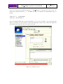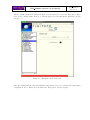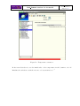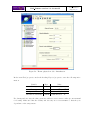
Download CodeSaturne version 1.3 tutorial

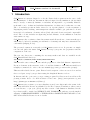
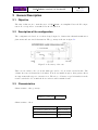
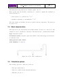
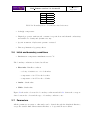
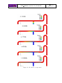
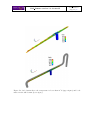
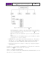
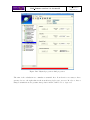
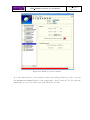
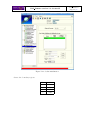
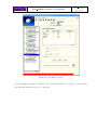
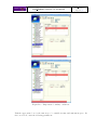
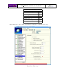
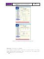
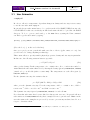
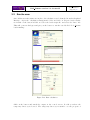
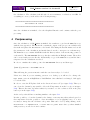
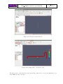
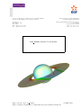
School of Mechanical, Aerospace and Civil Engineering
Faculty of Engineering and Physical Sciences
PO Box 88
Manchester, UK
M60 1QD
Fluid Dynamics, Power Generation
and Environment Department
Single Phase Thermal-Hydraulics Group
6, quai Watier
F-78401 Chatou Cedex
Tel: +44(0)161 306 9200
Fax: +44(0)161 306 3755
Tel: 33 1 30 87 75 40
Fax: 33 1 30 87 79 16
Code Saturne version 1.3.2 tutorial
http://rd.edf.com/code saturne
http://cfd.mace.manchester.ac.uk/twiki/bin/view/Saturne/WebHome
c EDF 2008
Code Saturne version 1.3.2 tutorial
Code Saturne
documentation
Page 2/33
TABLE OF CONTENTS
I
STRATIFIED JUNCTION
4
1
Introduction . . . . . . . . . . . . . . . . . . . . . . . . . . . . . . . . . . . . .
5
2
General Description . . . . . . . . . . . . . . . . . . . . . . . . . . . . . . . .
6
2.1
Objective . . . . . . . . . . . . . . . . . . . . . . . . . . . . . . . . . . . . .
6
2.2
Description of the configuration . . . . . . . . . . . . . . . . . . . . . .
6
2.3
Characteristics . . . . . . . . . . . . . . . . . . . . . . . . . . . . . . . . .
6
2.4
Mesh characteristics . . . . . . . . . . . . . . . . . . . . . . . . . . . . . .
7
2.5
Calculation options
. . . . . . . . . . . . . . . . . . . . . . . . . . . . . .
7
2.6
Initial and boundary conditions . . . . . . . . . . . . . . . . . . . . . . .
8
2.7
Parameters . . . . . . . . . . . . . . . . . . . . . . . . . . . . . . . . . . . .
8
2.8
Output management
. . . . . . . . . . . . . . . . . . . . . . . . . . . . . .
9
2.9
User routines . . . . . . . . . . . . . . . . . . . . . . . . . . . . . . . . . . .
9
. . . . . . . . . . . . . . . . . . . . . . . . . . . . . . . . . . . . . .
10
Step by step solution . . . . . . . . . . . . . . . . . . . . . . . . . . . . . . .
13
3.1
User Subroutine . . . . . . . . . . . . . . . . . . . . . . . . . . . . . . . . .
28
3.2
Run the case . . . . . . . . . . . . . . . . . . . . . . . . . . . . . . . . . . .
29
Postprocesing . . . . . . . . . . . . . . . . . . . . . . . . . . . . . . . . . . . .
30
2.10 Results
3
4
3
Part I
STRATIFIED JUNCTION
4
Code Saturne version 1.3.2 tutorial
1
Code Saturne
documentation
Page 5/33
Introduction
Code Saturne is a system designed to solve the Navier-Stokes equations in the cases of 2D,
2D axisymmetric or 3D flows. Its main module is designed for the simulation of flows which
may be steady or unsteady, laminar or turbulent, incompressible or potentially dilatable,
isothermal or not. Scalars and turbulent fluctuations of scalars can be taken into account.
The code includes specific modules, referred to as “specific physics”, for the treatment of
Lagrangian particle tracking, semi-transparent radiative transfer, gas, pulverized coal and
heavy fuel oil combustion, electricity effects (Joule effect and electric arcs) and compressible
flows. The code also includes an engineering module, Matisse, for the simulation of nuclear
waste surface storage.
Code Saturne relies on a finite volume discretization and allows the use of various mesh types
which may be hybrid (containing several kinds of elements) and may have structural nonconformities (hanging nodes).
The present document is a tutorial for Code Saturne version 1.3.2. It presents one simple
test case and guides the future Code Saturne user step by step into the preparation and the
computation of the case.
The test case directories, containing the necessary meshes and data are available in the
Code Saturne Kernel directory:
$CS HOME/doc/TUTORIAL/TEST CASES/STRATIFIED PIPE
This tutorial focuses on the procedure and the preparation of the Code Saturne computations.
For more elements on the structure of the code and the definition of the different variables, it
is highly recommended to refer to the user manual (type info_cs user at the prompt).
This tutorial is divided in two parts. First a brief description of the test case is done and in
the second part, a step by step solution using the Graphical Interface is done.
In this tutorial, the open source post-processing program ParaView is used as well as a 2D
plotting software Grace. See their websites for more info. (http://www.paraview.org and
http://plasma-gate.weizmann.ac.il/Grace/)
Code Saturne is free software; you can redistribute it and/or modify it under the terms of the
GNU General Public License as published by the Free Software Foundation; either version
2 of the License, or (at your option) any later version. Code Saturne is distributed in the
hope that it will be useful, but WITHOUT ANY WARRANTY; without even the implied
warranty of MERCHANTABILITY or FITNESS FOR A PARTICULAR PURPOSE. See the
GNU General Public License for more details.
Code Saturne version 1.3.2 tutorial
2
Code Saturne
documentation
Page 6/33
General Description
2.1
Objective
The aim of this case is to train the user of Code Saturne on a simplified but real 3D computation. It corresponds to a stratified flow in a T-junction.
2.2
Description of the configuration
The configuration is based on a real mock-up designed to characterize thermal stratification
phenomena and associated fluctuations. The geometry is shown on figure I.1.
Figure I.1: Geometry of the case
There are two inlets, a hot one in the main pipe and a cold one in the vertical nozzle. The
volumic flow rate is identical in both inlets. It is chosen small enough so that gravity effects
are important with respect to inertia forces. Therefore cold water creeps backwards from the
nozzle towards the elbow until the flow reaches a stable stratified state.
2.3
Characteristics
Characteristics of the geometry:
Diameter of the pipe Db = 0.40 m
Characteristics of flow:
Cold branch volume flow rate Dvcb = 4 l.m−1
Hot branch volume flow rate Dvhb = 4 l.m−1
Cold branch temperature
Tcb = 18.26◦ C
Hot branch temperature
Thb = 38.5◦ C
Code Saturne version 1.3.2 tutorial
Code Saturne
documentation
Page 7/33
The initial water temperature in the domain is equal to 38.5◦ C.
Water specific heat and thermal conductivity are considered constant and calculated at
18.26◦ C and 105 P a:
• heat capacity: Cp = 4, 182.88 J.kg −1 .◦ C−1
• thermal conductivity: λ = 0.601498 W.m−1 .◦ C−1
The water density and dynamic viscosity are variable with the temperature. The functions
are given below.
2.4
Mesh characteristics
The mesh used in the actual study had 125 000 elements. It has been coarsened for this
example in order for calculations to run faster. The mesh used here contains 16 320 elements.
Type: unstructured mesh
Coordinates system: cartesian, origin on the middle of the horizontal pipe at the intersection with the nozzle.
Mesh generator used: SIMAIL
Color definition: see figure I.2.
Figure I.2: Colors of the boundary faces
2.5
Calculation options
The following options are considered for the case:
→ Flow type: unsteady flow
→ Time step: variable in time and uniform in space
→ Turbulence model: k − Code Saturne version 1.3.2 tutorial
Code Saturne
documentation
Page 8/33
Colors Conditions
2
Cold inlet
6
Hot inlet
7
Outlet
5
Wall
Table I.1: Boundary faces colors and associated references
→ Scalar(s): temperature
→ Physical properties: uniform and constant for specific heat and thermal conductivity
and variable for density and dynamic viscosity
→ Specific treatment of hydrostatic pressure: activated
→ Time step limitation by gravity effects
2.6
Initial and boundary conditions
→ Initialization: temperature initialization at 38.5◦ C
The boundary conditions are defined as follows:
• Flow inlet: Dirichlet condition
– velocity of 0.03183 m.s−1 for both inlets
– temperature of 38.5◦ C for the hot inlet
– temperature of 18.6◦ C for the cold inlet
• Outlet: default value
• Walls: default value
Figure I.2 shows the colors used for boundary conditions and table I.1 defines the correspondance between the colors and the type of boundary condition to use.
2.7
Parameters
All the parameter necessary to this study can be defined through the Graphical Interface,
except the variable fluid characteristics that have to be specified in user routines.
Code Saturne version 1.3.2 tutorial
Code Saturne
documentation
Page 9/33
Parameters of calculation control
2.8
Number of iterations
100
Reference time step
1s
Maximal CFL number
20
Maximal Fourier number
60
Minimal time step
0.01 s
Maximal time step
70 s
Time step maximal variation
0.1
Period of output chronological files
10
Output management
The standard options for output management will be used. Four monitoring points will be
created at the following coordinates:
Points
1
2.9
X(m)
Y(m)
Z(m)
0.010025 0.01534 -0.011765
2
1.625
0.01534 -0.031652
3
3.225
0.01534 -0.031652
4
3.8726
0.047481
7.25
User routines
The following routines have to be copied from the folder FORT/USER/base into the folder
FORT1 :
• usphyv.F
This routine allows to specify variable physical properties, density and viscosity in particular.
In this case, the following variation laws are specified:
ρ = T.(A.T + B) + C
(I.1)
where ρ is the density, T is the temperature, A = −4.0668 × 10−3 , B = −5.0754 × 10−2 and
C = 1 000.9
For the dynamic viscosity, the variation law is:
µ = T.(T.(AM.T + BM ) + CM ) + DM
(I.2)
where µ is the dynamic viscosity, T is the temperature, AM = −3.4016 × 10−9 , BM =
6.2332 × 10−7 , CM = −4.5577 × 10−5 and DM = 1.6935 × 10−3
1
only when they appear in the FORT directory will they be taken into account by the code
Code Saturne version 1.3.2 tutorial
Code Saturne
documentation
Page 10/33
Note: in the user routines, the examples are protected by a test to prevent any undesired
use. Do not forget to deactivate them.
In order for the variable density to have an effect on the flow, gravity must be set to a non-zero
value. g = −9.81ey will be specified in the Graphical Interface.
2.10
Results
Figure I.3 shows the evolution of the temperature in the domain at different time steps. The
evolution of the stratification is clearly visible.
Figure I.4 shows the cells where the temperature is lower than 21◦ C. It is not an isosurface
created from the full domain, but a visualization of the full sub-domain created through the
post-processing routines.
Code Saturne version 1.3.2 tutorial
Figure I.3: Evolution of temperature
Code Saturne
documentation
Page 11/33
Code Saturne version 1.3.2 tutorial
Code Saturne
documentation
Page 12/33
Figure I.4: Sub-domain where the temperature is lower than 21◦ C (upper figure) and localization in the full domain (lower figure)
Code Saturne version 1.3.2 tutorial
3
Code Saturne
documentation
Page 13/33
Step by step solution
Before starting the Graphical Interface on Code Saturne, it is necessary to create the appropriate file structure for the code to work.
In order to allow all the scripts of Code Saturne to work properly, you will need to execute a
script to load all the environmental variables needed. Open a console and type:
( Note: [bash:$] in this document represents the prompt. It might be different depending
on your GNU-Linux installation and your profile file. There is no need to type this)
[bash:$] . /usr/local/Code_Saturne_1.3.2/Noyau/ncs-1.3.2/bin/cs_profile
This will load all the variables required (Note the dot ( . ) at the beginning of the command
line).
If everything went ok, you will now have an environmental variable called CS_HOME. To see
the value of this variable, type:
[bash:$] echo $CS_HOME
The output should be the path where the Code Saturne installation is located.
Now that you have your PATH updated, you can use the case creator script. Go to the desired
location on your directory and type:
[bash:$] cree_sat -etude STRATIFIED_JUNCTION K_EPS
This command will create a study called STRATIFIED_JUNCTION and a case called K_EPS. The
file structure can be seen in figure I.5
The details of the structure are:
• K EPS: This is the case file, a study can have several cases, for example different turbulence models, different boundary conditions etc.
– DATA: This is where the restarting files need to be copied, it also contains the
script to launch the Graphical Interface SaturneGUI.
– FORT: This is where the user subroutines are going to saved. During the compilation stage, the code will re-compile all the subroutines that are in this directory.
In the USERS directory all the user-defined subroutines are stored. For a specific
case you will only need a few of them depending on the changes that you want to
implement on the code. The base directory contains the basic flow solver subroutines, the other directories contain the subroutines needed by other modules such
Code Saturne version 1.3.2 tutorial
Code Saturne
documentation
Page 14/33
Figure I.5: File structure created by Code Saturne
as the Lagrangian, the combustion or the electric modules. For more information
on the other modules please see the ”Practical user guide to Code Saturne ” (you
can get it by typing info_cs user).
– RESU: Directory where the results will be exported once the calculation has finished.
– SCRIPTS: Here is were the launching scripts are copied. You will need to run the
executable file lance to start the calculation.
• MAILLAGE: The program will read the mesh from this directory. The mesh formats that can be read are I-DEAS, CGNS, Gambit Neutral files (neu), Ensigth, prostar/STAR4 (ngeom), Gmsh, NUMECA Hex, MED, Simail and Meta-mesh files.
• POST: This is an empty directory designed to contain post-processing macros (xmgrace,
experimental etc.)
You will need to copy the mesh into the MAILLAGE directory. The mesh can be found in the
installation of Code Saturne. At the prompt of the console type:
[bash:$] cd STRATIFIED_JUNCTION/MAILLAGE
[bash:$] cp $CS_HOME/doc/TUTORIAL/TEST_CASES/STRATIFIED_JUNCTION/MAILLAGE/sn_total.des .
(Note the dot ( . ) at the end of the line).
Code Saturne version 1.3.2 tutorial
Code Saturne
documentation
Page 15/33
Now, you can use the graphical interface of Code Saturne to complete the case set up. To
launch the graphical interface go to the DATA directory and launch the SaturneGUI script by
typing:
[bash:$] cd ../K_EPS/DATA
[bash:$] ./SaturneGUI &
Once the Graphical Interface is up and running, create a new case (File - Open New) and the
values of Identity and paths should be filled automatically. Click on the Solution Domain and
the mesh should appear selected as sn_total.des.
Figure I.6: Mesh Selection
Code Saturne version 1.3.2 tutorial
Code Saturne
documentation
Page 16/33
All the default parameters under Calculation environment are correct for this case so there
is no need to change them. Next go to Thermophysical models and under Turbulence models
select k − ε
Figure I.7: Turbulence model selection
Since the density and viscosity vary with the temperature, we need to activate the temperature
computation. Go to Thermal model and select Temprature (Celsuis degrees).
Code Saturne version 1.3.2 tutorial
Code Saturne
documentation
Page 17/33
Figure I.8: Temperature activation.
In the item Initialization, set the initial value of the temperature in the domain to 38.5◦ C.
Initialize the turbulence with the reference velocity 0.03183 m.s−1 .
Code Saturne version 1.3.2 tutorial
Code Saturne
documentation
Page 18/33
Figure I.9: Thermophysical models - Initialization
In the item Fluid properties, under the heading Physical properties, enter the following information:
Variable
Type
Value
Density
Variable
998.671 kg.m−3
Viscosity
Variable 0.445 × 10−4 kg.m−1 .s−1
Constant
4 182.88 J.kg −1 .◦ C−1
Thermal Conductivity Constant
0.601498 W.m−1 .K −1
Specific Heat
For density and viscosity, the value given here will serve as a reference value (see user manual
for details). Make sure that the density and viscosity are set as variable so that they are
dependant on the temperature.
Code Saturne version 1.3.2 tutorial
Code Saturne
documentation
Page 19/33
Figure I.10: Physical properties: fluid properties
The aim of the calculation is to simulate a stratified flow. It is therefore necessary to have
gravity. Set it to the right value in the item Gravity, hydrostatic pressure. In order to have a
sharper stratification, the pressure interpolation method will be set to improved.
Code Saturne version 1.3.2 tutorial
Code Saturne
documentation
Page 20/33
Figure I.11: Fluid properties - Gravity
Go to the item Definition and initialization under the heading Additional scalars to specify
the minimal and maximal values for the temperature: 18.26◦ C and 38.5◦ C. Note that the
initial value of 38.5◦ C set earlier is properly taken into account.
Code Saturne version 1.3.2 tutorial
Figure I.12: Scalar initialization
Create the boundary regions.
Colors Conditions
2
inlet
6
inlet
7
outlet
5
wall
Code Saturne
documentation
Page 21/33
Code Saturne version 1.3.2 tutorial
Code Saturne
documentation
Page 22/33
Figure I.13: Boundary regions
For the dynamic boundary conditions, the velocity is 0.03183 m.s−1 in the z direction and
the hydraulic diameter 0.4 m for both inlets.
Code Saturne version 1.3.2 tutorial
Code Saturne
documentation
Page 23/33
Figure I.14: Dynamic boundary conditions
For the scalar boundary conditions, the temperature of the cold inlet is 18.6◦ C and that of
the hot inlet is 38.5◦ C.
Code Saturne version 1.3.2 tutorial
Code Saturne
documentation
Page 24/33
Figure I.15: Temperature boundary conditions
Tick the appropriate box for the time step to be variable in time and uniform in space. In
the boxes below, enter the following parameters:
Code Saturne version 1.3.2 tutorial
Code Saturne
documentation
Page 25/33
Parameters of calculation control
Reference time step
1s
Number of iterations
100
Maximal CFL number
20
Maximal Fourier number
60
Minimal time step
0.01 s
Maximal time step
70 s
Time step maximal variation
0.1
And activate the option Time step limitation with the local thermal time step
Figure I.16: Time step
Code Saturne version 1.3.2 tutorial
Set the frequency of post-processing files to 10.
Create four monitoring probes at the following coordinates:
Points
1
X(m)
Y(m)
Z(m)
0.010025 0.01534 -0.011765
2
1.625
0.01534 -0.031652
3
3.225
0.01534 -0.031652
4
3.8726
0.047481
7.25
Code Saturne
documentation
Page 26/33
Code Saturne version 1.3.2 tutorial
Code Saturne
documentation
Page 27/33
Figure I.17: Outpput management and monitoring points
Important: Save the file before continuing.
Before running the calculation, fill the usphyv.F file to specify the variation of the density
and the viscosity with the temperature. Refer to the other cases or the example in the
TEST CASES directory for more information.
Code Saturne version 1.3.2 tutorial
3.1
Code Saturne
documentation
Page 28/33
User Subroutine
• usphyv.F
In order to allow for temperature dependant changes in density and viscosity, it is necessary
to use the user subroutine usphy.F.
In general, the user subroutines have to be copied from the folder FORT/USER/base into the
folder FORT2 . For this case, an already modified subroutine should be copied into the FORT
directory. To do so, open a console and go to the FORT directory using the Unix command
cd. Then copy the subroutine by typing:
[bash:$] cp $CS_HOME/doc/TUTORIAL/TEST_CASES/STRATIFIED_JUNCTION/CASE5/FORT/usphyv.F .
(Note the dot ( . ) at the end of the line).
Once you copied, you can open the file with your editor of choice (gedit, emacs, vi ...etc), but
you don’t need to change anything at this stage.
This routine allows to specify variable physical properties, density and viscosity in particular.
In this case, the following variation laws are specified:
ρ = T.(A.T + B) + C
(I.3)
where ρ is the density, T is the temperature, A = −4.0668×10−3 , B = −5.0754×10−2 and C =
1 000.9 Inside the subroutine this is done by altering the density (given by PROPCE(IEL,IPCROM)
) inside a loop on all cells (with a counter IEL). The temperature at each cell is given by
RTP(IEL,ISCA(1)).
For the dynamic viscosity, the variation law is:
µ = T.(T.(AM.T + BM ) + CM ) + DM
(I.4)
where µ is the dynamic viscosity, T is the temperature, AM = −3.4016 × 10−9 , BM =
6.2332 × 10−7 , CM = −4.5577 × 10−5 and DM = 1.6935 × 10−3
The dynamic viscosity if given by PROPCE(IEL,IPCVIS) for each cell IEL.
Note that this subroutine has been modified for this specific test case. In general, all user
subroutines are in FORT/USERS and they have examples for more general cases. Note: in the
user subroutines, the examples are protected by a test to prevent any undesired use. Do not
forget to deactivate them.
2
only when they appear in the FORT directory will they be taken into account by the code
Code Saturne version 1.3.2 tutorial
3.2
Code Saturne
documentation
Page 29/33
Run the case
Once all the user subroutines are in place, the calculation can be launched from the Graphical
Interface. Open the ’calculation management’ folder and click on ’Prepare batch calculation’.Click on the button labelled as ’Select the batch script file’ and select the ’lance’ file.
This will open new dialogues and give you the button to run the case labelled ’Code Saturne
batch running’.
Figure I.18: Run calculation
Click on the button and watch the output on the console screen. It tells you where the
temporary directory is located. The temporary directory is useful to see the progress of
Code Saturne version 1.3.2 tutorial
Code Saturne
documentation
Page 30/33
the calculation. The calculation should take about ten minutes on a Intel at 2.1 GHz. If
everything is correct, you should see the following message:
********************************************
Fin normale du calcul
********************************************
Once the calculation is finished, close the Graphical Interface and continue with the post
processing.
4
Postprocesing
Once the calculation of Code Saturne is finished, the results are copied in the RESU directory
with the date appended. The listenv file contains the output of the pre-processor which reads
the mesh and passes the information to the kernel. The listing file has information about all
the parameters of the calculation and useful data about the convergence at each time-step.
The HIST directory contains ASCII files with the history values of the monitoring points for
each variable. The CHR.ENSIGHT directory has the result files in EnSight format. These files
can be viewed with paraview directly. Additionally, a copy of the FORT directory and the lance
script used for the calculation are saved.
In order to visualise the results, go into the CHR.ENSIGHT directory and then type:
[bash:$] paraview --data=CHR.case &
This will bring the paraview interface with the case data ready to be loaded.
Please note that if you are running paraview on a desktop you will need to change the
Byte Order option from BigEndian to LittleEndian. Once this has been changed, click apply
to load the data.
In order to view the X-Z plane click on the direction button +Y (see figure I.20). Then you
can colour the domain by any variable. Select the Temperature from the box (see 2 in figure
I.20). This are the time dependat results, if you want to see the evolution, click on the play
button ( 3 in the figure I.20).
At the end you should have something similar to the figure I.22
It is also possible to colour the domain by the density or viscosity since their values depend on
the temperature. It is also possible to create streamlines or vectors (glyphs), but to do so it is
necessary to interpolate the cell data to the points. This can be done by using clicking on the
menu Filter --> Alphabetical --> Cell data to point data. Once you have finished
with paraview you can close it and continue.
Code Saturne version 1.3.2 tutorial
Code Saturne
documentation
Page 31/33
Figure I.19: Paraview initial window
Figure I.20: Temperature contours at 5.93s
The history files of all variables at the monitoring points can be seen in the HIST directory
under RESU. Go there and type
Code Saturne version 1.3.2 tutorial
Code Saturne
documentation
Page 32/33
Figure I.21: Temperatuse contours at 27.4s
[bash:$] gracehst Temp.C.hst
This script will start a 2D graphical program called grace (or xmgrace) and load the evolution
of the temperature over time at the chosen monitoring points. You should obtain something
like figure I.6
Code Saturne version 1.3.2 tutorial
Code Saturne
documentation
Page 33/33
Figure I.22: Temperatuse evolution at four monitoring points.