Download CodeSaturne version 1.3 tutorial

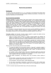
MSc/4th Year Aerospace Advanced CFD Laboratory
Laminar Flow in tube bundles
using Code Saturne
03/03/10
1
Introduction
Flows through tubes bundles are encountered in many heat exchanger applications. One
example is in nuclear power plants where the nuclear fuel rods are cooled by passing
cold water over them, but similar arrangements are also employed in more conventional
exchangers. The objective of this type of heat exchanger is, of course, to extract as much
heat as possible from the tubes. In a computational study, in order to calculate the heat
transfer reliably, it is necessary to resolve the flow around the tubes correctly.
A typical staggered tube bundle configuration, which is to be studied in this exercise,
can be seen in Figure 1. It is assumed to consist of a large number of tubes, so the flow
around any one is considered to be identical to that around the others. The computational domain employed is highlighted, which takes advantage of some of the symmetries
present in the flow. Symmetry conditions are applied on the top and bottom boundaries,
whilst periodic conditions (with a prescribed pressure drop) are applied between the east
and west boundaries.
Figure 1: Flow geometry
1
2
Laminar flow in tube bundles
The flow is to be computed as laminar, and three meshes are provided. The first
one consists of block structured quadrilateral cells with a resolution of 540 cells in total
with 72 points around one cylinder. The second mesh is an unstructured mesh made of
quadrilateral cells (PAVE). The total number of cells is 433 with 64 points around one
cylinder. The third mesh (TETRA) is mader of triagular elements, with a total number of
490 cells with 64 points around one cylinder. The meshes can be seen in Figure 2.
Figure 2: Three types of meshes
The use of a structured mesh means that there are rather highly skewed cells at the
interface between the curved edge of the cylinder and the straight symmetry edge. The
unstructured approach deals with this by removing the constraint of the cell edges having
to lie along the same lines as the block boundaries.
By using these relatively coarse meshes, the influence of the skewness of the grid can
be seen. Although the error introduced can be reduced by refining the mesh, the number
of cells required to reduce the error significantly is different for each meshing technique.
This means that before doing a mesh refinement study, it is often worth spending some
effort in achieving a grid structure with the least distortion possible.
A converged solution on a very fine grid is also available, allowing comparisons to
be drawn between these grid-independent results and those obtained on the three coarser
grids described above.
3
Laminar flow in tube bundles
2
Objectives
One of the objectives of this exercise is to compare the three different types of meshing techniques described above for a complex curved geometry, and assess their relative
strengths and weaknesses in terms of solution accuracy.
A second objective is to gain more experience in using a wider range of CFD and
other software tools for simulations and post-processing; in particular here using the
Code Saturne program to perform the flow simulations.
3
Investigations
First, follow the instructions given below to run the case using the block-structured grid
(BLOCK), and post-process the results. Then, follow the same steps to compute and
examine the solution for the other two grids.
Comparisons should be drawn between the computed solutions on the different grids,
and the grid-independent one from the provided fine grid solution. Qualitative comparisons can be made by examining velocity vector plots, contour plots of velocity or pressure, and streamlines. For quantitative output, useful comparisons include
• U -velocity component profiles along the periodic boundary (x = 0) and symmetry
line (y = 0).
• The flow recirculation length, deduced from the velocity profile along y = 0.
• The computed mass flow rate, conveniently expressed non-dimensionally as the
Reynolds number based on tube diameter and bulk velocity (Re = Ub d/ν).
• Compute the pressure drop coefficient Kp as in:
1
∆P = Kp ρUb2
2
(1)
The pressure drop ∆P/L = 10−5 has been set in the user subroutine ustsns.f90 as
a forcing term F = ∆P/L where L is the distance between the periodic faces.
OPTIONAL:
You could also investigate how the pressure drop coefficient Kp changes with Re
number. By systematically increasing the viscosity (multiply by 2, 4, 8 ...) you can
decrease Re while keeping the same ∆P . Calculate the quantity Kp Re and see if it
remains constant. How does the recirculation region change with Re?
4
Reporting Requirements
Students should submit a short report within 2 weeks of the laboratory. The report should
contain a brief introductory section, outlining the nature of the investigations conducted,
and should then describe and discuss (with the aid of a selection of figures) the results
obtained and comparisons between the various solutions. Excluding tables and figures
this is unlikely to require more than 4–5 pages of text.
Laminar flow in tube bundles
4
5 Code Saturne
Code Saturne is a system designed to solve the Navier-Stokes equations in the cases of
2D, 2D axisymmetric or 3D flows. Its main module is designed for the simulation of flows
which may be steady or unsteady, laminar or turbulent, incompressible or potentially
dilatable, isothermal or not. The code employs a finite volume discretisation and allows
the use of various mesh types, including hybrid arrangements (where the mesh contains
several kinds of elements) and structural non-conformities (hanging nodes).
The code includes specific modules, referred to as “specific physics”, for the treatment of Lagrangian particle tracking, semi-transparent radiative transfer, gas, pulverised
coal and heavy fuel oil combustion, electricity effects (Joule effect and electric arcs),
compressible flows, but these are not required for the present exercise.
Code Saturne is free software; it can be downloaded, modified and/or redistributed
under the terms of the GNU General Public License as published by the Free Software
Foundation.
The notes below guide you through the steps required to prepare and run the present
cases in Code Saturne version 2.0, and subsequently post-process the results using the
open-source post-processing program ParaView.
The meshes and data necessary for the exercise are available from the Manchester
CFD and Turbulence Modelling website at:
http://cfd.mace.manchester.ac.uk/Main/TubeBundleTutorial.
Further information on Code Saturne can be found in the user manual (accessed by
typing code_saturne info -g user at the prompt). More details of ParaView
can be obtained from the website http://www.paraview.org.
6
Guide to Running Code Saturne
Before starting the Graphical Interface on Code Saturne , it is necessary to create the
appropriate file structure for the code to work.
In order to allow all the scripts of Code Saturne to work, you will need to add the
path to the directory where the Code Saturne installation is located. Open a console
(Applications - Accessories - Terminal) and type:1
[bash:$] export PATH=$PATH:/opt/cs-2.0-rc2/bin
(Note: [bash:$] in this document represents the prompt. It might be different, depending on your GNU-Linux installation and your profile file. There is no need to type
this.)
The above command will load all the variables required (note the dot and space (. ) at
the beginning of the command line).
1
In a command line interpreter, such as bash, autocomplete of command names and file names may be
accomplished by keeping track of all the possible names of things the user may access. Here autocomplete
is usually done by pressing the Tab key after typing the first several letters of the word. For example, if
the only file in the current directory that starts with x is xLongFileName, the user may prefer to type x
and autocomplete to the complete name. If there were another file name or command starting with x in
the same scope, usually the user would have to type some more letters or press the Tab key repeatedly to
disambiguate what he or she means to the computer.
Laminar flow in tube bundles
5
If everything went OK, you should get the following information when typing code saturne:
[bash:$] code_saturne
Usage: /opt/cs-2.0-rc2/bin/code_saturne <topic>
Topics:
help
check_consistency
check_mesh
compile
config
create
gui
info
plot_probes
Options:
-h, --help
show this help message and exit
Now that you have your PATH updated, you can use the case creator script. You will
need about 150MB of free space, if your home directory has not enough space, use the
temporary directory on the machines, but be aware that you will need to copy your data
to other media as everything under /tmp will be deleted after reboot. Go to the desired
location (cd /tmp/ for example) and type:
[bash:$] code_saturne create --study TUBE_BUNDLE --case BLOCK
This command will create a study called TUBE_BUNDLE and a case called BLOCK.
The file structure can be seen in Figure 3
The details of the structure are:
• BLOCK: This is the case file. A study can have several cases, for example each
using different turbulence models, different boundary conditions, etc.
– DATA: This is where the restarting files need to be copied, it also contains the
script to launch the Graphical Interface SaturneGUI.
– SRC: This is where the user subroutines should be saved. During the compilation stage the code will re-compile all the subroutines that are in this directory.
In the REFERENCE directory all the user-defined subroutines are stored. For a
specific case you might only need a few of these, depending on what is needed
to implement the case. In this case we will make use of one such routine, in
order to prescribe a streamwise pressure drop between the periodic boundary
planes. The base directory contains the basic flow solver subroutines, the
other directories contain the subroutines needed by other modules.
– RESU: Directory where the results will be exported once the calculation has
finished.
– SCRIPTS: This is where the launching scripts are copied. You will need to
run the executable file runcase to start the calculation.
Laminar flow in tube bundles
6
Figure 3: File structure created by Code Saturne
• MESH: The program will read the mesh from this directory. The mesh formats
that can be read are I-DEAS, CGNS, Gambit Neutral files (neu), EnSight, prostar/STAR4 (ngeom), Gmsh, NUMECA Hex, MED, Simail and Meta-mesh files.
• POST: This is an empty directory designed to contain post-processing macros that
may be relevant for particular cases.
You will need to copy the mesh into the MESH directory. The mesh can be found on the
website: http://cfd.mace.manchester.ac.uk/Main/TubeBundleTutorial (This web address
is case sensitive)
Download the three meshes into the MESH directory. If your browser does not ask
you for a place to save the files try right clicking on the lick and select ’Save link as’.
Because the case is periodic in the streamwise direction, it is necessary to impose a
pressure gradient to make the flow move. To do this, download the file called ustsns.f90
from the above webpage and save it into the SRC directory. This file is a user subroutine
that adds source terms into the momentum equation. The file has already been edited for
this tutorial it is not necessary to change it.
Now, you can use the graphical interface of Code Saturne to complete the case set up.
To launch the graphical interface go to the DATA directory and launch the SaturneGUI
script by typing:
[bash:$] cd TUBE_BUNDLE/BLOCK/DATA
[bash:$] ./SaturneGUI &
7
Laminar flow in tube bundles
The graphical interface offers different folders that can be expanded by double clicking on them (see Figure 4). On the pages you can set all the values needed to run a
simulation. Once the Graphical Interface is up and running, create a new case (File New) and the values of Identity and paths should be filled in automatically. Open on
the Calculation environment folder and click on the Mesh selection page. The meshes
that you have downloaded into the MESH directory should appear in the box. Delete the
meshes that you are not going to use (i.e. leave only ROD BUNDLE BLOCK.neu)
Figure 4: Mesh Selection
Click on the periodic boundary conditions tab and set them up as a translation set.
Click on the Add button. A new panel will appear and in the List of boundary faces for
the selected periodicity click on New. Double click on the Groups box and type the groups
INLET and OUTLET Separated by a space. The translation vector is T X = 2, T Y = 0,
T Z = 0. See Figure 5.
Laminar flow in tube bundles
8
Figure 5: Periodic boundary conditions
Next, set the Thermophysical models. Click on the Calculation features page and
select Steady Flow. Click on the Turbulence model page and select no model, i.e. laminar
flow.
In the Physical properties folder, make sure the default properties of air are checked,
i.e. ρ = 1.17862 kg/m3 , µ = 1.83 × 10−5 Ns/m2 .
Next, expand the Boundary Conditions folder and click on the Definition of boundary
regions. Create the regions as shown in figure 6. Make sure there are no typos on the
localisation of the faces.
Then set the faces WALLR1, WALLR2 and WALLR3 as walls and the other as symmetry by clicking on each region and changing the Nature box, then click Modify.
Next, expand the Numerical parameters folder and in the Steady management page
set the number of iterations to 2000.
Finally, expand the Calculation management folder and click on the Prepare batch
calculation page. Click on the Select the batch script file button to select the runcase file.
The above step will open new dialogues and give you the button to run the case,
labelled ‘Code Saturne batch running’.
Important: Save the file as block.xml before continuing.
Click on the button and watch the output on the console screen. It tells you where
the temporary directory is located. The temporary directory is useful to see the progress
of the calculation. The calculation should take about two minutes on a Intel 2.1 GHz
processor. If everything is correct, you should see the following message:
9
Laminar flow in tube bundles
Figure 6: Boundary Conditions
********************************************
Normal simulation finish
********************************************
Once the calculation is finished, close the Graphical Interface and continue with the post
processing.
7
Post-Processing
Once the calculation of Code Saturne is finished, the results are copied into the RESU
directory with the date appended. The listpre file contains the output of the pre-processor
which reads the mesh and passes the information to the solver kernel. The listing file
has information about all the parameters of the calculation and useful data about the convergence at each time-step. The HIST directory contains ASCII files with the history of
monitored values for each variable. The CHR.ENSIGHT directory has the results files in
EnSight format. These files can be viewed with ParaView directly. Additionally, a copy
of the FORT directory and the runcase script used for the calculation are saved.
In order to visualise the results, go into the results directory by typing:
[bash:$] cd ../RESU/CHR.ENSIGHT.XXX’
where XXX is the date. Once inside the directory type:
10
Laminar flow in tube bundles
[bash:$] /opt/paraview-3.6.1/bin/paraview --data=CHR.case &
This will bring up the ParaView interface with the case data ready to be loaded.
click on apply to load the data.
Figure 7: ParaView initial window
By default the domain will be coloured by pressure contours. The variable used can
be changed via the top left corner box. The colouring scheme can also be set to a more
standard ‘blue-to-red’ scheme by clicking on the Edit color map button.
A quantitative way of comparing the results is to plot velocity profiles along particular
lines. For this exercise you can use the bottom symmetry line at y = 0 and the periodic
line at x = 0.
To plot a curve along the symmetry line, go to Filters - Alphabetical - PlotOverLine.
Select the points (0.5, 0 , 0.2) and (1.5,0,0.2) and the resolution to 20 points, then click
‘Apply’. A new window should appear with an XY plot of all variables. To select only the
streamwise velocity component, click on the ‘Display’ tab and tick only ‘VelocityU:X’ in
the list of variables.
To create another XY plot on the x = 0 plane, select the CHR.case box on the panel on
the left and repeat the procedure, but now using the points (0, 0.5, 0.2) and (0, 1, 0.2) and
a resolution of 10 points. Before clicking ’Apply’ make sure that you have the window
with the full domain selected (a red square around the window highlights the selected
one). If you have the window with the first XY plot selected, both lines will appear in the
same window. In the end your solution should be similar to what is shown in Figure 8 If
you want to export the values of a given line, selected from the pipeline browser panel on
the left and click on File - Save Data. This will open a new window where you can select
the name and the format. To save as text, use the .csv format (Comma Separated Values).
11
Laminar flow in tube bundles
This values can be imported into OpenOffice Calc (Similar to Microsoft Excel) or viewed
with a text editor such as gedit or emacs.
Figure 8: ParaView results
Many other postprocessing tools are available from ParaView. Some of these (such
as vectors or streamlines) require that the data be interpolated from the cell centres to the
nodes. To do this go to Filters - Alphabetical -CellToDataPoint. This will produce a new
data set with all the variables interpolated to the cell nodes, and other filters will then be
available.
NOTE: If you want to save a screenshot, you will need to change the default settings
to avoid paraview crashing. Go to Edit - Settings. Click on the ”Render View” in the
left pane and then uncheck ”Use offscreen for screenshots”. After you have changed the
setting you can save a screen shot by going to File - Save screen shot.
8
Fine Grid Solutions
After post processing the results for the BLOCK case, the same procedure can be applied
to the other two meshes, i.e. PAVE and TETRA. Create a new case for each mesh and
follow the same instructions. To move back a directory, use the cd .. command. To
list the contents of a directory type ls and to get the current working directory use pwd.
Once you are inside the TUBE_BUNDLE directory you can use the command
[bash:$] code_saturne create --case PAVE --case TETRA
to create two new cases inside the same study called PAVE and TETRA. After the cases
are created, you can proceed to open the graphical interface and fill in the values of each
case.
Laminar flow in tube bundles
12
After the results for the three meshes have been obtained, they can be compared with
the reference data available on the website. These results were obtained with a mesh of
30180 cells, and can be loaded into ParaView for comparison with the coarse mesh results
obtained during the exercise.