Download This paper says that the logical thing would be that the samples

This paper says that the logical thing would be that the samples should be measured again if the environment changes. They have studied six different environments in two cases: ‐
‐
The kNN from each sample were computed only among the other samples from the same environment (self – self). The kNN from each sample were computed using samples from all environments (self – all). They conclude that the self‐self case is better than the self‐all case in terms of accuracy, but the standard deviation of the self‐self case is noticeably larger than that of the self‐all case. They also study the K which provides the best results and they talk about the hardware they used, the protocol, the problems they found such us some ACK’s were lost, etc K-Nearest-Neighbor Analysis of Received Signal
Strength Distance Estimation Across Environments
Aaron Ault, Xuan Zhong, Edward J. Coyle
The Center for Wireless Systems and Applications
Purdue University, West Lafayette, Indiana 47907
Email: {ault,zhongx,coyle}@ecn.purdue.edu
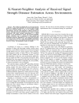
Abstract— Prior studies investigating the use of non-parametric
models for ranging and localization via received signal strength
have been restricted usually to one or two relatively similar
environments, and have used primarily to 802.11 network interfaces. This paper discusses methods for and results of ranging
experiments with signal strength measurements in a sensor
network as the environment is varied. The K-nearest-neighbor
distance estimation error is computed for both ranging and
localization scenarios. Degradation of the mean 80th percentile
error from 30 feet to 50 feet is seen when multiple environments
are considered; however, the standard deviation improves from
16 feet to 10 feet. The localization results are similar.
I. I NTRODUCTION
Localization of sensors is a common challenge in the
operation of indoor and short-range outdoor wireless sensor
networks. A cost-effective solution is to use the received signal
strength (RSS) across the wireless channel. Since mathematical propagation models of indoor RSS are still considered
both quite complex and not consistently accurate [1], most
RSS algorithms to date have used non-parametric approaches
that pre-sample the RSS in the operating environment. Many
algorithms have been proposed for this task, but the results of
[2] show that they all perform comparably due, most probably,
to inherent uncertainty in the environment.
Past work has shown a median (50th percentile) estimation
error of 9.64 feet [3], 10.4 feet [4], and 10 feet [2] when the
training samples were taken from the same environment as
the data samples. [3] found a median error of 14.1 feet for a
parametric approach, and [5] found a RMS error of 6 feet for
a different parametric approach in a dense network of sensors.
[2] shows that a median percentile error of 10 feet and a 97th
percentile error of 30 feet can be expected when using any
non-parametric algorithm on a pre-sampled environment.
Sampling an environment to train a non-parametric algorithm can be a time-consuming task. Furthermore, if the
environment changes after sampling, conventional logic would
say to re-sample the environment. We investigate the error that
might arise from a drastic change in environment without a
change in training samples.
We show in this paper that a good baseline for RSS based
algorithms in a MICA2-based sensor network is an 80th
percentile error of approximately 30 to 40 feet. A degradation
in accuracy of 20 feet is seen when a generic sample set from
multiple environments is used, but the variance of the error
decreases. We also discuss practical challenges of design and
implementation that we encountered during our experiment.
II. OVERVIEW
MPR400 MICA2 sensor motes from Crossbow [6] are used
for all experiments in this paper. They have a Chipcon CC1000
radio, which uses FSK modulation and provides a Received
Signal Strength Indicator (RSSI) output that is sampled by a
10-bit ADC. [7] All of our data was taken at 915.998 MHz.
TinyOS [8] was running on the motes and Sensor-MAC (SMAC) was used for communication. We developed a custom
algorithm for collecting and recording the data.
We recorded the output value of the RSSI for communications at 255 different power levels as the Physical Separation
Distance (PSD) was increased from 2 feet to 150 feet in
increments of 2 feet. Communication was not possible beyond
150 feet. We analyzed the resulting 255 dimensional dataset
using a leave-one-out K-nearest-neighbor (kNN) algorithm to
determine the cumulative distribution function (CDF) of the
distance estimation error. We also used the distance estimates
from the kNN analysis to simulate a localization problem
where a number of “beacon” motes, whose absolute locations
are known, are used to estimate the location of an unfixed mote
using only RSSI-based distance estimates to the beacons.
The leave-one-out kNN analysis followed [9]. It involves
taking one sample as a “data sample” and computing a
distance metric in the signal space to other samples, denoted
as “training samples.” The signal space distances (SSD) are
sorted, and the K samples with the smallest SSD are chosen
as the “K Nearest Neighbors.” The PSD’s for the kNN are
then combined to estimate the PSD of the data sample. This
is compared with the actual PSD to calculate the distance
estimation error. The cumulative distribution function (CDF)
of this error was plotted, along with the mean and standard
deviation of the CDF’s across environments. This analysis was
run in two scenarios: (1) the data sample was compared only
to training samples from its own environment (self-self); (2)
the data sample was compared to training samples from all
environments (self-all).
The localization algorithm took a random set of samples
from within one environment and placed them at random in
a 2-D plane such that they were located at the correct PSD
from an “unfixed” mote at the origin. Using the kNN estimated
PSD’s for the random set of samples, we minimized an error
function to estimate the unfixed mote’s location.
Samples were taken in 6 environments chosen for their variation in terms of contruction materials, architectural design,
and amount and type of “clutter.” We did not do any extensive
modeling to determine precise multipath and fading properties
because one purpose of this experiment is to determine how
well we can estimate PSD without complex environmental
studies. A description of each environment is given below,
along with some pictures in Figures 1 and 2.
A. Environment A
A 150 x 80 x 12 foot agricultural building housing 400 beef
cattle: The structure has an open ceiling and open 8-foot studs
sitting on top of 4-foot concrete sidewalls. The sensors were
located on a concrete driveway running down the middle of
the building that is flanked by cattle pens.
Fig. 1.
Set-up for taking samples in Environment C
B. Environment B
A 220 x 44 x 10 foot dairy building housing 120 dairy
cattle: The structure has a 10-foot, covered ceiling and open,
8-foot stud walls sitting on top of 2-foot concrete walls. There
is a large feed bunk in the middle of the barn that contains
conveyors and electric motors. The walls are lined with 8foot deep freestalls made of metal tubing and rubber floor
matresses. The sensors were located in the freestalls during
the experiment. Cattle were kept on the opposite side of the
feed bunk to safeguard the sensors.
C. Environment C
A 150 x 100 x 12 foot dairy building housing approximately
120 dairy cattle: The structure has steel I-beams running
straight up from the ground to a 12-foot eave, at which point
they angle inward and run the rest of the way up the roof. The
sides of the barn are open and the ends and roof are covered
with steel siding. A picture of the data capture setup for this
is shown in Figure 1. Some variations in this environment
were created by opening and closing garage doors, driving
tractors through the cattle pens, and by the presence of varying
numbers of cattle.
Fig. 2.
F. Environment F
An open, grassy field in West Lafayette, Indiana.
III. E XPERIMENTAL S ETUP
D. Environment D
A 44 x 20 x 8 foot milking parlor where dairy cattle
are milked: It is strikingly different from the other environments studied because the sensors did not have line-ofsight communication. The walls are made of ceramic-coated
concrete masonry blocks. The room is filled with large, angled,
stainless-steel obstructions designed to hold cattle. A picture
of this complex environment is in Figure 2.
E. Environment E
A 250 x 8 x 8 foot hallway on the third floor of the Materials
Science and Electrical Engineering (MSEE) building at Purdue
University: The most important feature of this environment is
the constant flow of people through the hallway.
Taking Samples in Environment D
This experiment was performed twice, with the second iteration containing all the improvements learned from experience
with the first. The challenges we encountered and our solutions
are presented in this section.
A. Hardware
The MICA2 motes were connected to an Apple Powerbook
G4 laptop using a MIB510 serial programming board from
Crossbow. The motes were set on cloth-topped camping tables
that were 1.25 feet tall. A plastic, 300-foot measuring tape was
used for measuring PSD and was kept stationary throughout
each experiment. A picture of the setup appears in Figure 1.
B. Network Protocols
The most important requirement placed on our network
protocol design comes from the kNN analysis. Any “missing”
data are assumed to be missing because the transmission power
was too low for communication. Therefore, the network must
not allow any data to be lost during transit.
We chose S-MAC over the standard TinyOS B-MAC protocol because B-MAC has a maximum packet payload size of
29 bytes, while S-MAC will allow up to 250 bytes. Our first
algorithm using B-MAC took 5 hours to take one sample at
each PSD; our final algorithm using S-MAC took 5 hours to
take 10 samples at each PSD, a factor of 10 improvement.
The largest source of error when using S-MAC was ACK’s
that were lost relatively frequently. One major drawback of
using larger packet sizes is that there can be no TCP-like
transport layer to guarantee delivery of all packets because
there is only 4 KB of RAM available to a program on
the motes (to prevent corruption of the call stack during
execution). This is not enough to store a number of large
packets for the purpose of retransmission. If smaller packets
are used, then retransmission buffers can be maintained in a
lower level of the communication stack.
It is important to note that this problem cannot be eliminated
simply by centralized polling by the computer. The signal
patterns of the MICA2 motes have distinct nulls that vary with
environment and can cause communication to be unreliable
even where one would expect it to be fine, thus allowing
ACK’s to be lost for reasons other than collisions.
Our final network algorithm involves a ring-like configuration of five sensor motes: the base, sender, receiver, sender
relay, and receiver relay.
The network configuration described below is used only
for collecting the data that is generated by the sender and
receiver. It was designed to ensure that no data is lost between
these two motes and the computer, and also to ensure that
there is little to no signal contention between motes during
the transmissions from the sender to the receiver. Our results
will hold for sensor grids of any density, provided the sensors
have been synchronized and avoid transmitting simultaneously.
If there are simultaneous transmissions, shadowing will occur,
and the results will likely be degraded.
C. Base
The base mote is attached to the programming board that
connects to the computer and is used to relay information
between the computer and the network. The communication
to the computer was handled through a custom serial interface
that we wrote for transferring arbitrarily large amounts of
information between the base station and a C program running
on the computer.
D. Sender
The sender mote waits to receive a control message from the
sender relay. The sender then transmits a “start message” to the
receiver and waits for a “ready message.” Then it broadcasts
sample packets at each of the 255 available transmission power
levels. A sample packet contains the transmitter battery voltage, the transmission power level, the PSD, and the sequence
number of this sample. Once the 255 transmissions have taken
place, a “done message” is sent to the receiver. If there are
more samples left to take at this PSD, then it repeats the
process again by sending another start message.
E. Receiver
The receiver mote waits for a start message from the sender.
It responds with a ready message if its sample buffer is empty.
Upon reception of a sample packet, it records the RSSI and its
own battery voltage level, as well as the information received
within the sample packet itself. It does this until a done packet
is received from the sender. It organizes the stored data into
“record messages” and sends them to the receiver relay for
delivery to the computer.
F. Sender Relay
The sender relay mote receives messages from the base on
the control port and retransmits them to the sender mote.
G. Receiver Relay
The receiver relay mote receives messages from receiver on
the record port, and retransmits them to the base station mote.
H. Miscellaneous Network Problems and Solutions
The existence of relay motes was an unanticipated need for
this experiment. We quickly learned that plugging the base
station mote into the programming board changes its communication characteristics such that it cannot communicate
beyond about 30 feet. We decided to create one relay mote
that could be moved easily to allow for longer communication
between the base station and the other motes. This still did
not fix the problem, as we would frequently experience cases
where the relay would have communication to either the sender
or the receiver, but not both. We therefore settled on the final
ring-like setup where each mote that must communicate with
the computer has its own relay.
In the end, our final algorithm had two main problems.
(1) ACK’s were still lost, causing some deadlock situations
between the sender and the recevier. After resetting the two
motes, the problem would be temporarily fixed. (2) The receiver and receiver relay would inexplicably enter states where
both were trying to send but neither was really doing anything.
If we waited for about one minute, then the transmission
would eventually go through and everything would resume.
Odd things would happen at this point on the computer, such as
multiple receptions of the same packet from the receiver relay,
and some packets that were sent were never received. After
resetting the two motes and repeating the sample, everything
usually worked correctly.
The lesson is that any algorithm we write in the future will
have a built-in reset message type that will instantly reset all
motes in the network, because manually resetting everything
when the motes are 150 feet apart wastes a lot of time.
TABLE I
A MOUNT OF DATA PER E NVIRONMENT
I. K-Nearest-Neighbor Analysis
We used Matlab to read all of the data files and separate
them into 255 dimension samples, where each transmitter
power level is one dimension. A summary of the amount of
data taken for each environment appears in Table I. We then
converted the RSSI readings from their raw ADC values to a
more meaningful dB value that factors in the receiver battery
power level using a formula provided in [7].
The squared Euclidean distance from each sample’s RSSI
values to all other samples was computed and sorted for each
sample in order to find the first K nearest neighbors in signal
space, for K from 1 to 100. We combined the PSD of the K
nearest neighbors as follows:
sk
wk = PKmax
j=1 sj
1
wk
ŵk = PKmax
j=1
dˆ =
KX
max
ŵk dk
k=1
1
wj
=
sk
1
PKmax
Eranging
j=1
Environment
Max. Distance
RSSI Measurements
255-D Samples
A
146
149,960
710
B
144
146,426
720
C
150
153,906
747
D
40
36,833
181
E
146
141,055
728
F
68
56,530
331
All
150
684,710
3417
The resulting setup was fed into the function:
f=
1
sj
¯
¯
¯
¯
= ¯dˆ − d¯
where wk is the weighting factor for neighbor k, sk is the
SSD of neighbor k, dˆ is the kNN distance estimate, dk is the
PSD of neighbor k, Eranging is the distance estimation error,
and d is the actual PSD of the data sample. We calculated
percentiles of the distance estimation error and plotted them
as a function of K in order to find the best K value.
Using the best K-value from above, we looked at two
different scenarios: where the kNN from each sample were
computed only among the other samples from the same
environment (self-self), and where the kNN for each sample
were computed using samples from all environments (selfall). These curves were plotted for each environment, and then
the mean and standard deviation of these curves were plotted
against each other.
After plotting the CDF’s for each environment, it became
clear that the environments where the maximum PSD was
small performed artificially well; their maximum possible error
was much smaller than that of the other environments. To make
a valid comparison, we normalized each of the CDF curves
by the maximum PSD of each environment.
J. Localization Algorithm
Using the kNN distance estimates, we then separated the
data in each file into sets of samples with the same PSD.
Then, generating a random permutation of the available PSD’s
in each environment, we selected one of the samples at random
for each of the distances in the permuation.
In order to simulate an environment where stationary beacon
motes are transmitting to an unfixed mote, we placed the
unfixed mote at the origin (0,0) of a 2-D plane. Then, each
of the samples chosen from the random permutation were
assigned a uniformly random number from zero to 2π. The
beacon motes were then placed at their PSD from the origin
but with with the random polar angle.
N ¯
¯
X
¯
¯
2
2
¯(xi − x̂) + (yi − ŷ) − dˆ2i ¯
i=1
where N is the number of beacon motes, xi and yi are the
known x and y coordinates of beacon i, x̂ and ŷ are the
unknown x and y coordinates of the unfixed mote, and dˆi
is the kNN estimated distance from beacon i to the unfixed
mote.
The function f is then minimized over x̂ and ŷ to result
in an estimate of the unfixed mote’s location.
The location
p
error was computed as: Elocalization = x̂2 + ŷ 2 Note that
the actual coordinates of the unfixed mote do not appear in
the Elocalization equation because they are (0,0).
IV. R ESULTS
Our final data set contained 3417 samples of 255 RSSI
values from 6 environments. We took 10 samples at each
PSD except for the final distance where communication failed
before 10 samples could be taken. The indoor, line-of-sight
environments allowed communication nearing 150 feet due
to waveguide effects, whereas the outdoor and non-line-ofsight environments lost communication at 68 and 40 feet. A
summary of the amount of data taken is given in Table I.
Figure 3 shows the results of our attempts to find the best
value for K. As expected, the 50th, 80th, and 90th percentile
curves all start to approach a constant value around K = 9
or 10. Our weighting method weights the neighbors that are
closer in signal space more heavily than those far away. As K
increases, we are adding more neighbors that are farther away,
so their contribution to the end result is smaller and smaller.
[3] used a simple direct averaging weighting scheme, and they
saw heavy degradation in performance as K became large. We
plotted both schemes, and they performed almost identically
for small K values, but the final scheme we used was clearly
superior for larger values of K. We chose K = 9 for the rest
of our analysis because it is near the steady-state values, but
is also small enough to speed up computation.
Using K = 9, we plotted the CDF of the distance estimation
error for the self-self case (Figure 4) and the self-all case
(Figure 5) for each environment. For the self-self case, each
Percentiles of Distance Estimation Error for Self−All vs. K
CDF of Distance Estimation Errors from Each Environment to Entire Data Set
90
80
Error Distance (ft) At Each Percentage
1
50th Percentile
80th Percentile
90th Percentile
K=9
0.9
70
0.8
60
0.7
50
0.6
0.5
40
Env. A (146 ft max)
Env. B (144 ft max)
Env. C (150 ft max)
Env. D ( 40 ft max)
Env. E (146 ft max)
Env. F ( 68 ft max)
All Environments
0.4
30
0.3
20
0.2
10
0.1
0
0
Fig. 3.
10
20
30
40
50
K value
60
70
80
90
100
10
20
30
40
50
60
70
Error in Estimated Distance (ft)
80
90
100
50th, 80th, and 90th Percentile Values vs. K for Self-All Case
Fig. 5.
CDF of Distance Estimation Errors for Self-All Scenario
CDF of Distance Estimation Errors From Each Environment To Itself
1
artificially poor performance by including nearest neighbors
with PSD’s that are outside the realm of possibility for that
environment.
In order to better investigate the degradation in performance
due to using a generic set of samples, we computed the mean
and standard deviation of the curves in both cases and plotted
them in Figure 6.
0.9
0.8
0.7
0.6
0.5
0.4
0.3
0.2
Env. A (146 ft max)
Env. B (144 ft max)
Env. C (150 ft max)
Env. D ( 40 ft max)
Env. E (146 ft max)
Env. F ( 68 ft max)
All Environments
Mean and Mean +/− Std of CDFs Across Environments
1
0.9
0.8
0.1
0
0
Fig. 4.
0.7
0.1
0.2
0.3
0.4
0.5
0.6
Error in Estimated Distance (% of Maximum Distance in Set)
0.7
CDF of Distance Estimation Errors for Self-Self Scenario
0.6
0.5
0.4
curve was normalized by the maximum PSD for that environment, so that the x-axis of the CDF plots are actually in units
of percentage of maximum communication distance. In other
words, if the desired environment allows for communication
up to 100 feet, then the x-axis should be scaled by multiplying
by 100. Note that this is only valid for ranges on the order of
those studied here.
The self-self plot resembles the results of [2], as expected.
The open field and milking parlor were the best environments
for this case. This is probably because they were both static –
no moving people, animals or objects during the experiment.
It is also possible that our method of dividing the error by
the maximum PSD in the set does not fully account for the
problem of smaller maximum possible error.
The self-all plot, however, shows the open field and milking
parlor environments to be by far the worst of the environments.
The smaller maximum PSD in each set is probably leading to
Mean, Self−Self
Mean + 1 Std, Self−Self
Mean − 1 Std, Self−Self
Mean, Self−All
Mean + 1 Std, Self−All
Mean − 1 Std, Self−All
0.3
0.2
0.1
0
0
Fig. 6.
ments
0.1
0.2
0.3
0.4
0.5
Distance Estimation Error (% of Maximum Distance)
0.6
Mean CDF +/- 1 Std of Distance Estimation Error Across Environ-
It is obvious from Figure 6 that the self-self case is better
than the self-all case in terms of accuracy, but the standard
deviation of the self-self case is noticeably larger than that of
the self-all case.
If we assume that a standard environment allows for
communication up to 150 feet, then we expect to be able
to predict the PSD between two sensor motes with 80%
Mean CDF +/− 1 Std of Localization Error for 3 and 25 beacons
are very high, about 130% of the maximum ranging error.
This is due to the poorer kNN distance approximations that
can be seen in Figure 5. All of the curves seem to follow an
exponential decay, showing that more beacons in general leads
to better accuracy, agreeing with the results from [4].
80th Percentile vs. Number of Beacons
70
60
80th Percentile (feet)
confidence to within 30 feet if the samples are taken from the
same environment, and 50 feet if the samples are taken from
generic environments. The self-self case has an 80th percentile
standard deviation of 16.1 feet, and the self-all case has an 80th
percentile standard deviation of 9.8 feet, an improvement of
almost 40%.
At first, the improvement in precision seems counterintuitive. To understand this result, one must think further
about what it means to have a smaller standard deviation in the
context of a kNN estimate. If we look at a sample (sample A)
with a PSD of 6 feet, for instance, we will get one estimate of
the distance based on the other samples around it. If we have
another sample (sample B) at 6 feet that is relatively close in
signal space to sample A, then B’s estimate will be ”far” from
A’s only if a small change in signal space location results in
a very different set of neighbors. ”Different” in the sense that
the new neighbors have much different PSD’s than those of the
neighbors of the first sample. Therefore, a highly-irregularly
populated signal space will lead to a high standard deviation.
We expect that the overall signal space of the self-all case will
be more regularly populated than the self-self case due to the
much larger number of samples from somewhat similar sets.
Environment A
Environment B
Environment C
Environment D
Environment E
Environment F
50
40
30
20
5
Fig. 8.
1
10
15
20
Number of Beacons
25
30
Localization Error vs. Number of Beacons
0.9
V. C ONCLUSION
0.8
We conclude that received signal strength is a mediocre
estimator for ranging and localization in general sparse sensor
networks, with modest accuracy improvements possible if the
operating environment has been pre-sampled.
0.7
0.6
0.5
VI. ACKNOWLEDGEMENTS
0.4
Mean, 3 Beacons
Mean + 1 Std, 3 Beacons
Mean − 1 Std, 3 Beacons
Mean, 25 Beacons
Mean + 1 Std, 25 Beacons
Mean − 1 Std, 25 Beacons
0.3
0.2
0.1
0
This research was funded in part by a Tellabs Fellowship
and by the Indiana 21st Century Research and Technology
Fund under Award #1110030618.
0
Fig. 7.
20
40
60
80
Location Estimation Error (feet)
100
R EFERENCES
120
Mean CDF +/- 1 Std of Localization Error for 3 and 25 Beacons
Figure 7 shows the mean localization error CDF +/- 1
standard deviation across all environments. Comparing this
plot to the ranging error in Figure 6, one can see that the
localization CDF is much steeper than that of the ranging
algorithm. This is because the random placement of beacon
motes allows for some ranging errors to effectively cancel
out other ranging errors. However, this results in a much
larger standard deviation than with ranging. The mean 90th
percentile is smaller using localization, but the 80th is larger.
The mean 80th percentile error was 36.97 feet, and the
standard deviation was 17.95 feet for 25 beacons across all
environments.
The effect of the number of beacons on accuracy is plotted
in Figure 8. The open field and milking parlor error estimates
[1] N. Priyantha, A. Chakraborty, and H. Balakrishnan, “The cricket locationsupport system,” Boston, MA, Aug. 2000, [Online] Available: http:
//citeseer.ist.psu.edu/priyantha00cricket.html.
[2] E. Elnahrawy, X. Li, and R. P. Martin, “The limits of localization using
signal strength: A comparative study,” Santa Clara, CA, Oct. 2004, [Online] Available: http://paul.rutgers.edu/∼eiman/elnahrawy04limits.pdf.
[3] P. Bahl and V. N. Padmanabhan, “Radar: An in-building user location
tracking system,” vol. 18, Boston, MA, Aug. 2000, [Online] Available:
http://citeseer.ist.psu.edu/bahl00radar.html.
[4] P. Krishnan, A. Krishnakumar, W.-H. Ju, C. Mallows, and S. Ganu,
“A system for lease: Location estimation assisted by stationary emitters
for indoor rf wireless networks.” Oct. 2000, [Online] Available: http:
//citeseer.ist.psu.edu/642879.html.
[5] N. Patwari, A. Hero, M. Perkins, N. Correal, and R. O’Dea, “Relative
location estimation in wireless sensor networks,” IEEE Trans. Signal
Processing, vol. 51, no. 8, pp. 2137–2148, Aug. 2003, [Online] Available:
http://citeseer.ist.psu.edu/591597.html.
[6] (2004) The crossbow website. [Online]. Available: http://www.xbow.com
[7] MPR/MIB User’s Manual, Crossbow, 2004, [Online] Available:
http://www.xbow.com/Support/Support pdf files/MPR-MIB Series User
Manua%l 7430-0021-06 A.pdf.
[8] (2004) The tinyos website. [Online]. Available: http://www.tinyos.net
[9] K. Fukunaga, Introduction to Statistical Pattern Recognition.
San
Francisco: Morgan Kaufman, 1990.