1
TIME-2008 Symposium
Technology and its Integration in Mathematics Education
10th ACDCA Summer Academy
8th Int’l Derive & TI-NspireConference
Hosted by the Tshwane University of Technology
22-26 September 2008, Buffelspoort conference centre, South Africa
Teaching Mathematics with CAS to Future Engineers:
Some Examples of What We (Absolutely) Need
Michel BEAUDIN
Ecole de technologie supérieure
1100, Notre-Dame street West, Montreal (Quebec) Canada
[email protected]
ABSTRACT
We are teaching mathematics at Ecole de technologie supérieure (ETS), an
engineering school in Montréal, Canada where every student has a Voyage 200 calculator
on his desk and has access to computer labs where CAS like Derive, Maple and also
Matlab program are installed. In Vienna (Visit-me 2002), we showed many examples of
how Derive 5 and the TI-92 Plus were used when teaching to engineering students. For
the past 4 years, we used the Voyage 200 and Derive 6.10 for teaching single and
multiple variable calculus, linear algebra, differential equations, complex analysis. The
talk will show examples of the importance of 2D implicit plotting, 3D plotting and Ode’s
plotting when teaching to future engineers. These features are not yet implemented into
Nspire and we hope that it will be on board soon. If we agree that we have to make a
move from Derive to Nspire, we don’t agree to leave higher mathematics subjects to the
competitors.
1. Introduction
Nspire processor is so fast that it would be nice to have access to these important features
⎯ in fact this is an absolute necessity ⎯ that are used daily in engineering mathematics. We do
know that slope fields plotting and numerical RK method will be available soon for Nspire. Let
us hope that not only slope fields, but direction fields for systems of Odes will be available. At
present time, the solving facilities of Nspire CAS are robust and accurate: when we need to find
critical points of a 2 variables function f, there is no problem at all for solving the system
∇f = [ 0, 0] ⎯ especially if f is a polynomial ⎯ but we don’t have access to level curves
plotting, neither 3D plotting. The examples, presented in the next section, will be done using
“good old” Derive 6.10. Let us recall (from Derive User Manual, version 3, 1994) that Derive is
a “tireless, powerful, and knowledgeable mathematical assistant, it is an easy, natural and
convenient tool”. This is what we are expecting from Nspire CAS software, not less. A good
mathematics teacher does not need to look at his papers when he is giving a course: the same
should be done when he is using a CAS. With Derive, you can teach naturally, without having to
loose your time with complicated commands.
We will focus on the following:
a) We need implicit 2D plotting, 3D plotting (especially parametric 3D plotting); we also need
numerical differential equations plotting. Al of these will be illustrated in examples 2.1 and 2.2.
b) We need slider bar: Nspire version 1.4 has it but we need time to take a look at it. Also, we
were so well served by the ability of Derive to integrate piecewise continuous functions that we
just can’t understand why this is not carried over Nspire. All of these will be illustrated in
example 2.3.
c) Voyage 200 has many 2D plot windows, not only one. This can also be an advantage.
Example 2.4 will show this.
d) Finally, the 14 digits limitation for computation is not acceptable at university level. No
example will be presented here ⎯we showed good ones at DERIVE-NSPIRE Transition
Conference in Austria in April 2007⎯ but this limitation represents another illustration of leaving
higher mathematics subjects to the competitors.
2
This document will never be able to show exactly what we lost with the discontinuation
of Derive. Those who will be attending the talk at the conference will have the opportunity to see
that Derive was ⎯ let it say again ⎯ a “tireless, powerful, and knowledgeable mathematical
assistant, an easy, natural and convenient tool”.
2. Some examples
Example 2.1: when we are using TI-Nspire CAS (handheld/software) in order to find
and classify the critical of an expression containing 2 independent variables, we can’t use plotting
facilities (we could with Voyage 200 but it is very slow due to the processor ⎯ this is why TINspire CAS handheld should add implicit 2D plots and 3D plots). Of course, we always have the
possibility of finding (some) critical points by using the solving facilities and calculus (first and
second order derivatives). Let us illustrate this with f ( x, y ) = x 4 − xy 2 + 3 y 3 − 5 y . In order to
know the nature of these 2 critical points, we can do further investigations, using multiple
variable calculus functions like the Hessian matrix (here we use self-programmed functions:
“ptcri” gives the matrix of the critical points of f and “nature” gives the vector
⎡⎣ H (a, b), f xx'' (a, b) ⎤⎦ where H is the Hessian matrix). The next figures show that there are 2
critical points; the critical point in the first quadrant is a minimum while the one in the fourth
quadrant is a saddle point. It would have been nice to have access at some “Gröbner basis”
function in order to understand why all critical points have been found.
Figure 1a
Figure 1b
“We don’t want to leave higher mathematics level to the competitor” we just said at the end of
our abstract. Implicit 2D plotting is easily done in Derive and points defined inside a matrix can
be plotted: this is how we produced figure 2a (the 2 critical points along with the curves
3
∂f
∂x
= 0,
∂f
∂y
= 0 and figure 2b (the 2 critical points with some level curves). Using Voyage 200,
only one implicit 2D curve can be plotted because we need to use the 3D plot window and only
one surface can be checked at the same time. Level curves shown in figure 2b can be achieved
with the Voyage 200, but it will take a very long time. With Nspire, no implicit 2D plot is
available for the moment.
Figure 2a
Figure 2b
Now, the 2 corresponding points (in the space) with the surface defined by z = f(x, y) (figure 2c).
Figure2c
4
Finally, the critical points were found by solving the following system:
⎧4 x3 − y 2 = 0
⎨
2
⎩ −2 xy + 9 y − 5 = 0
Our students won’t solve this by hands. The “rref” command (“row_reduce” in Derive) used to
solve linear systems is replaced by the lexical Gröbner/Buchberger elimination method. Voyage
200 and TI-Nspire use this method but no such function is available. Let’s use again Derive: see
figure 3 where we are “convinced” that the there are only 2 critical points:
Figure 3
Example 2.2: since the last 3 or 4 years, students, in multiple variable calculus, are often
asked to find parametric equations for the curve of intersection of 2 surfaces and, using a CAS, to
plot both surfaces and the curve in the same window. When they see that the curve lies on both
surfaces, they are confident that the parametric equations they have found are correct…
Of
course, the parametric representation is not unique, so if we find one representation ⎯ using
some algebraic techniques for example ⎯ , we will be able to plot the 3D curve using a CAS like
Derive or Maple for example. But Voyage 200 has no 3D curves plotting and, as we said earlier,
only one surface can be plotted in a single window. And if we can’t find parametric equations,
there is always a possibility to generate this curve numerically, using an ODE numeric solver for
G
dr
= ∇f × ∇g where the equations f = 0 and g = 0 define the 2
the ODE system given by
dt
G
dr
is the tangent vector to the curve.
surfaces, and
dt
5
Here is a concrete example. We plot the great circle when the sphere x 2 + y 2 + z 2 = 25 intersects
the plane x + y + z = 0 . Setting z = 0 in both equations gives one point on the curve. The
following Derive session does the job (and if you plot #7, you get the space curve!):
Figure 4
Of course, everything, here, can be done exactly. We have x 2 + y 2 + ( − x − y ) 2 = 25 , so
x + y + xy =
2
x+
2
y
2
=
25
2
25
2
cos t ,
2
y ⎞ 3y
25
⎛
⇒ ⎜x+ ⎟ +
=
. Using the first trigonometry identity, we can set
2⎠
4
2
⎝
3
4
y=
25
2
2
sin t . A possible exact representation is:
⎧
5 2
5 6
cos t −
sin t
⎪x =
2
6
⎪
⎪
5 6
sin t
0 ≤ t ≤ 2π
⎨y =
3
⎪
⎪
5 2
5 6
cos t −
sin t
⎪z = −
2
6
⎩
The sphere is plotted using spherical coordinates and not implicit 3D plot that has never been
available in Derive: that was and is again a good reason to use also DPGraph!.
Figure 5
6
Example 2.3: Nspire version 1.4 has a slider bar. This is a must because, at any level,
this can be used to illustrate many concepts. Some Derive users did not have the chance to look
at the one implemented in Derive 6 and we will consider the following example, from differential
equations: a mass-spring problem is governed by a differential equation, namely
m
d2y
dy
+ b + ky = f (t ),
2
dt
dt
y (0) = y0 , y′(0) = v0 .
In the classroom, we prove some of the following results, choosing for convenience m = 1. The
actual document can’t be a substitute for an illustration of the slider bar, so some results are not
shown here.
a) When the rhs is 0, we have damped motion called over damped case when b 2 − 4k > 0 ,
critically damped case when b 2 − 4k = 0 and under damped case when b 2 − 4k < 0 . This can
be seen rapidly, fixing for instance b to 4 and letting k vary from 1 to 10.
b) When the rhs is a periodic sine force, the initial conditions have no effect on the behaviour of
the entire solution because it becomes a steady-state solution with the same period as the input
force.
c) When the rhs is a non trivial periodic force, use of Fourier series is usually done but, because
Derive can integrate piecewise continuous functions, we can use a command (dsolve2 in Derive)
and produce a graph of the solution in a few seconds! A simple Derive function can be used to
produce concrete examples. In earlier conferences, we showed that the indicator function along
with the modulo function can be used to produce any non trivial periodic function. Here is an
example: if the input is the periodic wave defined by
⎧1 if 0 < t < 2
f (t ) = ⎨
⎩ −3 if 2 < t < 4
P=4
and if the initial conditions are 0 and if we take for b the value 4 and for k the value 1, then the
output can be plotted in a 2D plot window without having to simplify the solution obtained by the
command sol(4, 1, f(t), 0, 0). We only have to get the periodic extension. In the figure 6, a
Derive session with only 4 commands shows all of this: the “sol” function can be used for the
slider bar, fixing all parameters, except one (or more if we want!). Line #3 defines the periodic
7
function f above and line #4 is simply the (not simplified) solution of the ODE!!! Graphs of the
input f and output (the solution) are shown in figure 7: we can recognise rapidly the steady-state
solution of period 4 and can see that the solution passes through the point (0, 0) with a 0 slope
(because of the initial conditions). When you show this live to your students, you don’t have to
load any prepared file: you simply do “live mathematics on the computer”. This was (and still
remains) a driving force of Derive.
Figure 6
Figure 7
Example 2.4: Voyage 200 has different types of 2D plot windows and this can be turned
into an advantage instead of being a problem. Nspire 2D plot window can deal with explicit plot,
parametric plot, polar plot and scatter plot, all in the same window: for the calculator (handheld),
I am not convinced that this is a good idea. Putting everything in the same 2D plot window
makes it overloaded. Voyage 200 has 5 separate 2D plot windows (function, parametric, polar,
sequence and differential equations) and scatter plot can be done also, using Data/Matrix APPS.
Let us repeat: we think that, for a calculator ⎯ even with a large screen as for Voyage 200 or
8
Nspire ⎯ , we should not ONLY have a single 2D plot window for everything. It is difficult to
see everything and, as mathematics teaching is concerned, this is a very different story when you
are dealing with y = f(x) functions and parametric equations for instance. Of course, with no
implicit 2D plot window ⎯ except if you switch to 3D but only one curve can be plotted at the
time ⎯, Voyage 200 has many limitation when comes time to solve systems of 2 equations
containing 2 variables (using the “solve” command is always possible, but “seeing” the solutions
is also important). So, in order to show why different 2D plot windows are important, let us
conclude our examples with the following. Some months ago, I asked these 2 questions to my
students. First question: using your Voyage 200 calculator, find the solutions of the following
system of polynomial equations
⎧⎪ x3 + y 3 = 10
⎨ 2 2
⎪⎩ xy − x y = 2
and show the solutions in a 2D plot window. Using the 2D Function plotting window, they had to
do some algebra! In fact, the solved both equation for y and plotted the 3 curves in the same
window: when COMPLEX FORMAT was set at RECTANGULAR, they get only “one cubic
root” for the first equation and if it was set at REAL, they get the entire curve defined by the first
equation but not the entire curve defined by the second equation!!! Using the F5 Math menu ⎯ it
seems that we lost this in Nspire ⎯, they found the 3 intersections (and they were happy!).
Second question: 2 objects move in the xy plane according to the parametric following equations:
⎧⎪ x = 2 − t 2
C1 : ⎨
3
⎩⎪ y = 3t − t
( 0 ≤ t ≤ 1)
⎧ x = 3sin s
C2 : ⎨
2
⎩ y = 5s − 2 cos s
( 0 ≤ s ≤ 1)
Plot both trajectories in the same window and find the coordinates of the point of intersection of
the curves C1 and C2 . Students observed that, in parametric mode, there is no “intersection”
item in the F5 Math menu ⎯ because the first object reaches the point of intersection at a
different time from the second one ⎯, so they had to use a solve command for 2 equations in 2
unknowns (t and s) and discovered the importance of solving with a starting point (if you solve
2 − t 2 = 3sin s and 3t − t 3 = 5s 2 − 2 cos s , Voyage 200 finds a value of s and/or t outside the
interval [0, 1]!) So, the different 2D plot windows help me, as a math teacher, to make the
9
difference between the types of plotting we are using. Of course, when we are using a computer
(e.g. Derive on the PC), a single 2D plot window does not represent the same problem.
3. Conclusion
For the past 9 months, with many colleagues at ETS (Ecole de technologie supérieure),
we talked a lot about Nspire CAS. Our situation, at ETS, is probably unique in North America:
every engineering student has his own Voyage 200. This is a fantastic opportunity to use
computer algebra in the classroom, without the problems generated by personal computers in the
classroom: and, when a computer is needed because they have to use Derive, Maple or Matlab,
students can go to the lab or use their own personal computer. Now, personally, I am facing the
following problem: Derive is discontinued and many colleagues are afraid that Voyage 200
operating system won’t be updated. One thing is sure: we will probably not ask our new students
to buy Nspire CAS handheld because the QWERTY keyboard of Voyage 200 is so pleasant and
we do need “a university level package”. And, if we decide that every student has to bring a
laptop in the classroom, we will use Maple (Matlab for non mathematicians) and not Nspire CAS
software. For this reason, Texas Instruments should continue the development of Voyage 200, in
particular, by updating the operating system and adding a new processor. Finally, on a purely
personal note, the more I use Derive, the more I like it. Does it make sense to own computer
software without doing anything with it?
Of course, the interface is old and would need
improvements. But the math engine is unique. I am not still convinced that Nspire CAS software
will be a true successor of Derive. Two years later after the Dresden conference, I have the
feeling that the discontinuation of Derive was not a good move. I am still convinced that
something can be done with Derive. The competitors are strong but we should not let them win
the game. Only time will tell.
10