Download César Emanuel Brandão Gomes Monitorização Fina do - Serv-CPS

Departamento de
Universidade de Aveiro Electrónica, Telecomunicações e Informática
2012
César Emanuel
Brandão Gomes
Monitorização Fina do Consumo de Energia Eléctrica
Fine Grained Monitoring of Electric Energy
Consumption
Departamento de
Universidade de Aveiro Electrónica, Telecomunicações e Informática
2012
César Emanuel
Brandão Gomes
Monitorização Fina do Consumo de Energia Eléctrica
Fine Grained Monitoring of Electric Energy
Consumption
Dissertação apresentada à Universidade de Aveiro para cumprimento dos
requisitos necessários à obtenção do grau de Mestre em Engenharia Electrónica e Telecomunicações, realizada sob a orientação científica do Professor
Doutor Paulo Bacelar Reis Pedreiras, Professor Auxiliar do Departamento de
Electrónica, Telecomunicações e Informática da Universidade de Aveiro e do
Professor Doutor Alexandre Manuel Moutela Nunes da Mota, Professor Associado do Departamento de Electrónica, Telecomunicações e Informática
da Universidade de Aveiro.
Trabalho financiado por Fundos Nacionais através da “FCT - Fundação para
a Ciência e a Tecnologia” no âmbito do projecto “Serv-CPS” PTDC/EAAAUT/122362/2010
Trabalho financiado pelo programa Europeu FEDER através do “Programa
Operacional Factores de Competitividade - COMPETE” e pelo Governo
Português através da “FCT - Fundação para a Ciência e a Tecnologia” no
âmbito do projecto “HaRTES” FCOMP-01-0124-FEDER-007220
o júri / the jury
presidente / president
Professor Doutor José Alberto Gouveia Fonseca
Professor Associado da Universidade de Aveiro
vogais / examiners committee
Professor Doutor Paulo José Lopes Machado Portugal
Professor Auxiliar da Faculdade de Engenharia da Universidade do Porto
Professor Doutor Paulo Bacelar Reis Pedreiras
Professor Auxiliar da Universidade de Aveiro
Professor Doutor Alexandre Manuel Moutela Nunes da Mota
Professor Associado da Universidade de Aveiro
agradecimentos /
acknowledgements
Gostaria de agradecer ao Professor Doutor Paulo Pedreiras a sugestão
deste tema de dissertação, o qual desde o início me interessou por ser de
elevada praticabilidade e ligação ao mundo real. Agradeço em conjunto aos
Professor Doutor Paulo Pedreiras e ao Professor Doutor Alexandre Mota
pela excelente orientação que me proporcionaram.
Agradeço a todos os que me acompanharam no meu percurso académico,
nos meus altos e baixos. Agradeço a quem me acompanhou nas minhas
inúmeras discussões, e me ajudou a estimular o meu raciocínio e a questionar
o mundo que me rodeia.
Gostaria também de agradecer aos meus pais por me proporcionarem a
oportunidade de realizar este curso numa área que me cativa e num local
onde me sinto confortável. Agradeço tambem pela excelente educação que
me proporcionaram e pelos valores que me transmitiram.
Agradeço ainda à Micro I/O Serviços de Electrónica, LDA pela cedência
dos uMRFs sem os quais não poderia ter feito a rede de sensores sem fios
para medição indirecta de potência.
Palavras-chave
Monitorização Não Intrusiva de Cargas, Redes de Sensores sem Fios, Medição Indirecta de Potência
Resumo
Hoje em dia assistimos a uma grande pressão e esforço no sentido de estimular a conservação de energia, seja devido a limitações económicas, preocupações ambientais, ou normas regulatórias. No topo do consumo de
energia está a energia sob a forma de electricidade
Para se conseguir incentivar a utilização eficiente da energia é necessário
fornecer consciencialização energética. Se os consumidores de elecricidade
tiverem acesso a informação detalhada sobre como, quando e que aparelhos estão a consumir energia, estes poderão tomar boas e bem suportadas
decisões e anuir mudar os seus hábitos de modo a reduzir o consumo de
energia, e por fim, gastar menos dinheiro.
O projecto aqui apresentado desenvolve as bases para um aparelho que
fornece informação detalhada sobre o consumo de energia eléctrica para
uma casa. A informação a ser fornecida deverá ser separada individualmente
para virtualmente cada aparelho singular presente.
A técnica escolhida para desenvolver o aparelho foi Monitorização Não Intrusiva de Cargas de Aparelhos. A partir de um único ponto de medida o
sistema deverá identificar as cargas individuais na casa, o que faz com que
o hardware tenda a ser simples e minimal, recaindo a complexidade para
o software. O sistema desenvolvido deverá ser de baixo custo e de fácil
instalação.
O sistema que foi desenvolvido foi capaz de identificar individualmente e
com grande sucesso os aparelhos presentes num ambiente controlado. Ao
contrário de outros sistemas deste tipo, o sistema apresentado nesta dissertação é capaz de distinguir cargas eletricamente idênticas, através do uso
da técnica de Medição Indirecta de Potência implementada através de uma
Rede de Sensores Sem Fios.
Keywords
Non-Intrusive Appliance Load Monitoring, Wireless Sensor Networks, Load
Disambiguation, Indirect Power Sensing
Abstract
Nowadays we witness a great pressure and effort in order to stimulate energy
conservation, either due to economic constraints, environmental concerns,
or regulatory pressures. At the top of the energy consumption is the consumption of energy in the form of electricity.
The first step to improve energy utilization efficiency is energy awareness.
So if there is some manner to provide the average person information about
how he is consuming electricity, he may take it by its own interest, and In
fact, if electricity consumers have access to detailed information about how,
when and by which devices energy is consumed, they can make good and
well supported decisions on how they can change their habits to spend less
energy and ultimately spend less money.
The project hereby presented, develops the basis for a device that provides
detailed information on electrical energy expenditure for a home. The information to be provided aims to be disambiguated for virtually every individual
appliance present.
The chosen technique to develop such a device was Non-Intrusive Appliance Load Monitoring. The system identifies individual loads from a single
measurement point. That makes that the hardware tends to be simple and
minimal, passing the complexity to the software. The system aims to be
very low cost and easy to deploy.
The system developed was able to identify with great success individual
appliances in the total load on a controlled environment. Unlike other
systems of this type, the system presented in this dissertation has the ability
of disambiguating electrically identical loads, by the use of the technique of
Indirect Power Sensing deployed with a Wireless Sensor Network
Contents
Contents
i
List of Figures
iii
List of Tables
vii
List of Acronyms
ix
1 Introduction
1.1 Motivation . . . . . . . . . . . . . . . . . . . . . . . . . . . . . . . . . . . . .
1.2 Proposition . . . . . . . . . . . . . . . . . . . . . . . . . . . . . . . . . . . . .
1.3 Document Outline . . . . . . . . . . . . . . . . . . . . . . . . . . . . . . . . .
1
1
1
2
2 Analysis of Non-Intrusive Appliance Load Monitoring
2.1 Definition . . . . . . . . . . . . . . . . . . . . . . . . . .
2.2 Total Load Model . . . . . . . . . . . . . . . . . . . . .
2.3 Appliance Models . . . . . . . . . . . . . . . . . . . . . .
2.4 Signatures . . . . . . . . . . . . . . . . . . . . . . . . . .
2.5 NIALM Process . . . . . . . . . . . . . . . . . . . . . . .
2.6 Known Limitations . . . . . . . . . . . . . . . . . . . . .
2.7 Indirect Power Monitoring WSN . . . . . . . . . . . . .
2.8 Summary . . . . . . . . . . . . . . . . . . . . . . . . . .
.
.
.
.
.
.
.
.
.
.
.
.
.
.
.
.
.
.
.
.
.
.
.
.
.
.
.
.
.
.
.
.
.
.
.
.
.
.
.
.
.
.
.
.
.
.
.
.
.
.
.
.
.
.
.
.
.
.
.
.
.
.
.
.
.
.
.
.
.
.
.
.
.
.
.
.
.
.
.
.
.
.
.
.
.
.
.
.
.
.
.
.
.
.
.
.
3
3
3
5
7
10
13
13
14
3 System’s Architecture and Hardware Development
3.1 System’s Architecture . . . . . . . . . . . . . . . . .
3.2 Deployment of Data Acquisition System . . . . . . .
3.3 Communicating with the Data Acquisition System .
3.4 SPI-PC Gateway Implementation . . . . . . . . . . .
3.5 Wireless Sensor Network Nodes . . . . . . . . . . . .
3.6 Deployment of Indirect Power Sensing . . . . . . . .
3.7 Summary . . . . . . . . . . . . . . . . . . . . . . . .
.
.
.
.
.
.
.
.
.
.
.
.
.
.
.
.
.
.
.
.
.
.
.
.
.
.
.
.
.
.
.
.
.
.
.
.
.
.
.
.
.
.
.
.
.
.
.
.
.
.
.
.
.
.
.
.
.
.
.
.
.
.
.
.
.
.
.
.
.
.
.
.
.
.
.
.
.
.
.
.
.
.
.
.
15
15
17
21
23
30
31
35
.
.
.
.
37
37
41
45
50
4 Software Implementation
4.1 Load Disambiguation and Appliance Classification
4.2 Preliminary Validation of the Load Disambiguation
4.3 Preliminary Algorithm’s Software Implementation
4.4 Fine Grained Electricity Monitor . . . . . . . . . .
i
.
.
.
.
.
.
.
.
.
.
.
.
.
.
. . . . . . .
Algorithm
. . . . . . .
. . . . . . .
.
.
.
.
.
.
.
.
.
.
.
.
.
.
.
.
.
.
.
.
.
.
.
.
.
.
.
.
4.5
Summary . . . . . . . . . . . . . . . . . . . . . . . . . . . . . . . . . . . . . .
5 Tests, Results, Validations and Calibrations
5.1 Test-bed . . . . . . . . . . . . . . . . . . . . .
5.2 Calibration . . . . . . . . . . . . . . . . . . .
5.3 Appliance Characterization . . . . . . . . . .
5.4 Testing the Load Disambiguation Algorithm .
5.5 Complete System Test and Validation . . . .
5.6 Summary . . . . . . . . . . . . . . . . . . . .
62
.
.
.
.
.
.
65
65
67
74
75
81
83
6 Conclusions and Future Work
6.1 Conclusions . . . . . . . . . . . . . . . . . . . . . . . . . . . . . . . . . . . . .
6.2 Future Work . . . . . . . . . . . . . . . . . . . . . . . . . . . . . . . . . . . .
85
85
86
Appendix A Available Electric Monitoring Integrated Solutions
A.1 Analog Devices - ADE7953 . . . . . . . . . . . . . . . . . . . . .
A.2 Microchip’s MCP3909 . . . . . . . . . . . . . . . . . . . . . . . .
A.3 Maxim’s 78M6613 . . . . . . . . . . . . . . . . . . . . . . . . . .
A.4 Continental Control Systems - WattNode ModBus . . . . . . . .
A.5 Microchip’s PIC18F87J72 Single-Phase Energy Meter - Energy
PICtail Plus Daughter Board . . . . . . . . . . . . . . . . . . . .
89
89
91
93
96
Appendix B Current Sensing Technologies
B.1 Low Resistance Current Shunts . . . . .
B.2 Current Transformer . . . . . . . . . . .
B.3 Hall Effect Current Sensor . . . . . . . .
B.4 Rogowski Coil Sensor . . . . . . . . . . .
B.5 Prices Survey . . . . . . . . . . . . . . .
.
.
.
.
.
.
.
.
.
.
.
.
Survey
. . . . .
. . . . .
. . . . .
. . . . .
. . . . .
.
.
.
.
.
.
.
.
.
.
.
.
.
.
.
.
.
.
.
.
.
.
.
.
.
.
.
.
.
.
.
.
.
.
.
.
.
.
.
.
.
.
.
.
.
.
.
.
.
.
.
.
.
.
.
.
.
.
.
.
.
.
.
.
.
.
.
.
.
.
.
.
.
.
.
.
.
.
.
.
.
.
.
.
.
.
.
.
.
.
.
.
.
.
.
.
.
.
.
.
.
.
.
.
.
.
.
.
.
.
.
.
.
.
.
.
.
.
.
.
.
.
.
.
.
.
.
.
.
.
.
.
.
.
.
. . . . . . .
. . . . . . .
. . . . . . .
. . . . . . .
Monitoring
. . . . . . .
.
.
.
.
.
.
.
.
.
.
.
.
.
.
.
.
.
.
.
.
.
.
.
.
.
.
.
.
.
.
.
.
.
.
.
96
99
99
100
101
103
105
Appendix C Transimpedance Current Sensor with Current Transformer
107
Appendix D Light Sensor Circuit
111
Appendix E Current and Magnetic Field
115
Appendix F UART Protocol
117
Appendix G Indirect Current Sensor
119
Bibliography
123
ii
List of Figures
2.1
2.2
2.3
2.4
2.5
3.1
3.2
3.3
3.4
3.5
3.6
3.7
3.8
3.9
3.10
3.11
3.12
3.13
3.14
3.15
Simple representation of home’s electrical circuit . . . . . . . . . . . . . . . .
Finite State Appliance Models: (a) generic 1000 W two-state appliance; (b) no
frost refrigerator; (c) three-way Lamp; (d) clothes dryer; (e) three-speed fan.
Based on figure 4 of [18] . . . . . . . . . . . . . . . . . . . . . . . . . . . . .
Steady-State complex power signature space of some household appliances [18]
NIALM process . . . . . . . . . . . . . . . . . . . . . . . . . . . . . . . . . . .
Detection of Steps . . . . . . . . . . . . . . . . . . . . . . . . . . . . . . . . .
4
6
9
11
12
16
19
20
21
22
23
24
25
26
26
28
29
30
31
3.17
3.18
3.19
System’s architecture overview . . . . . . . . . . . . . . . . . . . . . . . . . .
CR8349 Current Transformer . . . . . . . . . . . . . . . . . . . . . . . . . . .
ADE7953 evaluation board I/O . . . . . . . . . . . . . . . . . . . . . . . . . .
Load System Configuration . . . . . . . . . . . . . . . . . . . . . . . . . . . .
Minimal data transaction . . . . . . . . . . . . . . . . . . . . . . . . . . . . .
chipKit Max32 development board [7] . . . . . . . . . . . . . . . . . . . . . .
SPI gateway implementation . . . . . . . . . . . . . . . . . . . . . . . . . . .
SPI Packet . . . . . . . . . . . . . . . . . . . . . . . . . . . . . . . . . . . . .
Gateway Write . . . . . . . . . . . . . . . . . . . . . . . . . . . . . . . . . . .
Gateway Read . . . . . . . . . . . . . . . . . . . . . . . . . . . . . . . . . . .
Gateway Read Alternative . . . . . . . . . . . . . . . . . . . . . . . . . . . . .
UART protocol basic packet . . . . . . . . . . . . . . . . . . . . . . . . . . . .
Gateway Dataflow . . . . . . . . . . . . . . . . . . . . . . . . . . . . . . . . .
uMRFs wireless node[5] . . . . . . . . . . . . . . . . . . . . . . . . . . . . . .
Light Sensor: a) - Light Sensor Circuit Schematic; b) - Assembled Sensor
Circuitry . . . . . . . . . . . . . . . . . . . . . . . . . . . . . . . . . . . . . .
Magnetic Flux around a two Conductor Cable: a) -Cut-section of a generic two
conductor cable; b) - Magnetic Flux vs Angle . . . . . . . . . . . . . . . . . .
SS39 Series Linear Hall Effect Sensors[42] . . . . . . . . . . . . . . . . . . . .
Block Diagram for indirect current sensing . . . . . . . . . . . . . . . . . . . .
Fully Assembled Version of Indirect Current Sensor Circuit . . . . . . . . . .
4.1
4.2
4.3
4.4
4.5
4.6
Load Disambiguation Algorithm Representation . . . . . . .
Representation of the filter for step detection . . . . . . . .
Steps and Signatures on the P-Q plane . . . . . . . . . . . .
Pass of Standard Deviation window through the Real Power
Representation of Steady State Identification . . . . . . . .
Representation of Step Identification . . . . . . . . . . . . .
37
40
41
43
43
44
3.16
iii
. . . . . . .
. . . . . . .
. . . . . . .
of an Oven
. . . . . . .
. . . . . . .
.
.
.
.
.
.
.
.
.
.
.
.
.
.
.
.
.
.
32
33
34
35
35
4.7
4.8
4.9
4.10
4.11
4.12
4.13
4.14
4.15
4.16
4.17
4.18
4.19
4.20
4.21
5.1
5.2
5.3
5.4
5.5
5.6
5.7
5.8
Preliminary Implementation of the NILM system . . . . . . . . . . . . . . .
Appliance Identification in mains aggregated load: a) - Refrigerator Detection;
b) - Oven Detection; c) - Refrigerator and Oven Detection . . . . . . . . . .
Fine Grained Electricity Monitor and its logical entities . . . . . . . . . . . .
Data Acquisition Logical Entity . . . . . . . . . . . . . . . . . . . . . . . . . .
Step-Detection entity . . . . . . . . . . . . . . . . . . . . . . . . . . . . . . . .
Appliance Classification Process . . . . . . . . . . . . . . . . . . . . . . . . .
Data-logging entity . . . . . . . . . . . . . . . . . . . . . . . . . . . . . . . . .
WSN Representation . . . . . . . . . . . . . . . . . . . . . . . . . . . . . . . .
Indirect Power Sensing WSN entity representation . . . . . . . . . . . . . . .
Graphical User Interface entity . . . . . . . . . . . . . . . . . . . . . . . . . .
Graphical User Interface default appearance . . . . . . . . . . . . . . . . . . .
Graphics with traces of RMS Voltage and RMS Current . . . . . . . . . . . .
Graphics with traces of the components of complex power of Total Power and
Estimated Power . . . . . . . . . . . . . . . . . . . . . . . . . . . . . . . . . .
Informations about the electrical installation . . . . . . . . . . . . . . . . . .
Apps Tab of Graphical User Interface . . . . . . . . . . . . . . . . . . . . . .
System’s electric installation testbed: a) - block diagram, b) - physical instalation
Light Sensor Placement . . . . . . . . . . . . . . . . . . . . . . . . . . . . . .
Placement of magnetic sensor . . . . . . . . . . . . . . . . . . . . . . . . . . .
Appliance Classification in I-Q plane . . . . . . . . . . . . . . . . . . . . . . .
Appliances’ Individual Interval of identification - a . . . . . . . . . . . . . . .
Appliances’ Individual Interval of identification - b . . . . . . . . . . . . . . .
Histograms of the delay between the detection by the WSN and by the loaddisambiguation algorithm . . . . . . . . . . . . . . . . . . . . . . . . . . . . .
Comparison of Measured Power with Estimated Power . . . . . . . . . . . .
A.1
A.2
A.3
A.4
A.5
A.6
ADE7953 functional block diagram [4] . . . . . . . . . . . . . . . . . . . . . .
ADE7953 Evaluation board [14] . . . . . . . . . . . . . . . . . . . . . . . . . .
MPC3909 Functional block diagram [30] . . . . . . . . . . . . . . . . . . . . .
MCP3909/dsPIC33F 3-Phase Meter Reference Design [29] . . . . . . . . . . .
78M6613 Functional block diagram[2] . . . . . . . . . . . . . . . . . . . . . .
78M6613 Evaluation Boards:(a)78M6613 - EVM - Evaluation Board[1],
(b)78M6613SP - EVM - Split Phase Evaluation Board[3] . . . . . . . . . . . .
A.7 WattNode connection schematic [44] . . . . . . . . . . . . . . . . . . . . . . .
A.8 Microchip’s PIC18F87J72 Energy Monitoring PICtail[33] . . . . . . . . . . .
B.1
B.2
B.3
B.4
B.5
B.6
B.7
B.8
B.9
Current shunt simple model . . . . . . . . . . . . . . . .
Examples of Current Shunt Resistors[9] . . . . . . . . .
Simple model of a Current Transformer . . . . . . . . .
Examples of Current Transformers . . . . . . . . . . . .
Hall effect principle[19] . . . . . . . . . . . . . . . . . . .
Hall effect principle, magnetic field present[19] . . . . .
Simplified linear current sensor[19] . . . . . . . . . . . .
Hall effect linear current sensor[41] . . . . . . . . . . . .
Rogowski Coil current sensor, simple representation[11]
iv
.
.
.
.
.
.
.
.
.
.
.
.
.
.
.
.
.
.
.
.
.
.
.
.
.
.
.
.
.
.
.
.
.
.
.
.
.
.
.
.
.
.
.
.
.
.
.
.
.
.
.
.
.
.
.
.
.
.
.
.
.
.
.
.
.
.
.
.
.
.
.
.
.
.
.
.
.
.
.
.
.
.
.
.
.
.
.
.
.
.
.
.
.
.
.
.
.
.
.
.
.
.
.
.
.
.
.
.
48
49
50
51
52
53
54
56
57
59
60
60
60
61
62
66
72
73
77
78
79
80
82
89
91
91
92
94
95
96
97
99
100
100
101
101
102
102
103
103
B.10 Examples of Rogowski Coil current sensors . . . . . . . . . . . . . . . . . . .
104
C.1 Simple model of a Current Transformer . . . . . . . . . . . . . . . . . . . . .
C.2 Current Sensor Circuit . . . . . . . . . . . . . . . . . . . . . . . . . . . . . . .
C.3 Current Sensor Board . . . . . . . . . . . . . . . . . . . . . . . . . . . . . . .
107
108
109
D.1 Light Sensor basic Circuit . . . . . . . . . . . . . . . . . . . . . . . . . . . . .
D.2 Light Sensor Circuit Schematic . . . . . . . . . . . . . . . . . . . . . . . . . .
D.3 Assembled Sensor Circuitry . . . . . . . . . . . . . . . . . . . . . . . . . . . .
111
112
113
E.1 Current carrying conductor . . . . . . . . . . . . . . . . . . . . . . . . . . . .
115
F.1 UART Write Message . . . . . . . . . . . . . . . . . . . . . . . . . . . . . . .
F.2 UART Read Message . . . . . . . . . . . . . . . . . . . . . . . . . . . . . . . .
F.3 Gateway Fata Message . . . . . . . . . . . . . . . . . . . . . . . . . . . . . . .
117
117
118
G.1 Hall-Effect Sensor Conditioning Circuit . . . . . . . . . . . . . . . . . . . . .
G.2 Schematic of the Indirect Current Sensor Circuit . . . . . . . . . . . . . . . .
G.3 Fully Assembled Version of Indirect Current Sensor Circuit . . . . . . . . . .
119
121
122
v
vi
List of Tables
3.1
3.2
3.3
Systems’ main features . . . . . . . . . . . . . . . . . . . . . . . . . . . . . .
Comparative of the various solutions for current measurment . . . . . . . . .
Register’s adressing scheme . . . . . . . . . . . . . . . . . . . . . . . . . . . .
18
19
22
4.1
4.2
Single Appliance Characterization of some appliances in REDD . . . . . . .
Comparison of detection in single appliance files to detection in aggregated
load mains file . . . . . . . . . . . . . . . . . . . . . . . . . . . . . . . . . . .
45
Assertion of gain error following the calibration of voltage channel
Assertion of gain error following the calibration of current channel
Results of the voltage meter constant fitting . . . . . . . . . . . . .
Results of the current meter constant fitting . . . . . . . . . . . . .
Appliance’s Characterization . . . . . . . . . . . . . . . . . . . . .
Results of Single Appliance tests on step-detector . . . . . . . . . .
Appliance classification tolerances . . . . . . . . . . . . . . . . . .
Analysis of the delay in the WSN detection . . . . . . . . . . . . .
Detection of appliances in a random sequence of events . . . . . .
Comparison of Norms of Power Values . . . . . . . . . . . . . . .
Energy Values by integration of Power Flows . . . . . . . . . . . .
.
.
.
.
.
.
.
.
.
.
.
68
69
71
72
74
75
76
80
81
82
82
C.1 Current Sensor Circuit Bill of Materials . . . . . . . . . . . . . . . . . . . . .
108
5.1
5.2
5.3
5.4
5.5
5.6
5.7
5.8
5.9
5.10
5.11
vii
.
.
.
.
.
.
.
.
.
.
.
.
.
.
.
.
.
.
.
.
.
.
.
.
.
.
.
.
.
.
.
.
.
.
.
.
.
.
.
.
.
.
.
.
.
.
.
.
.
.
.
.
.
.
.
48
viii
List of Acronyms
NIALM Non-Intrusive Appliance Load Monitoring
WSN Wireless Sensor Network
NILM Non-Intrusive Load Monitoring
FSM Finite State Machine
SFD
Start of Frame Delimiter
EFD
End of Frame Delimiter
MSb most significant bit
MSB most significant byte
GUI
Graphical User Interface
ix
x
Chapter 1
Introduction
1.1
Motivation
Nowadays we witness demanding economical and regulatory pressures for the deployment
of energy efficient technologies, to promote energy’s conservation. The reasons behind this
interest are the reduction of carbon dioxide emissions as in Kyoto’s Protocol, the reduction of
costs, and ultimately the ambient conservation, by reducing the consumption of fossil fuels.
One of the most, if not the most, used energy form is electrical energy, thus it arises
the need to reduce the electrical energy being spent in industrial, commercial and home
environments.
One way of promoting this reduction is giving energy awareness to electricity consumers,
giving them feedback on how and where the energy is being spent. Some studies state that
direct feedback on energy consumption can lead to savings between 10 to 15% in the electrical
bill [20].
To provide energy awareness there’s the need of a fine grained energy monitor capable of
monitoring the majority of appliances within a household environment, individually. There
are two main ways of accomplishing this. The first consists in deploying one sensor at each
appliance to be monitored and measure directly the power being spent by it, recording the
desired data. This technique presents the drawbacks of being very expensive and difficult to
install, as it requires intrusion and modification of the house’s electrical circuit. Further it
can be very difficult to monitor appliances that don’t allow direct physical access, such as
embedded ovens. The second is a concept introduced in 1992 by George W. Hart, that is NonIntrusive Appliance Load Monitoring a technique for monitoring the electrical consumption
of individual appliances of a household facility without the necessity of installing individual
sensors for each appliance. By sophisticated analysis of current and voltage of the total
load, ideally at the main panel circuit breaker, it is estimated the number and nature of the
individual loads and their individual energy consumption, as well as other relevant statistics.
The hardware cost of this implementation is comparatively very low, turning the complexity
to the software [18].
1.2
Proposition
It is hereby proposed the development of a fine grained energy monitor capable of monitoring the majority of appliances within a household environment based on Non-Intrusive
1
Appliance Load Monitoring. The system ought to provide direct feedback, in real time, by
showing the total power being spent as well as what appliances are turned ON, and historical
feedback by doing with electricity what is done with the telephone bill, i.e., discriminating in
detail how the energy was spent, what appliances were in function and when, and how much
energy they were spending and its cost.
Although a Non-Intrusive Appliance Load Monitoring (NIALM) system may identify different appliances within the total load, there is a clear limitation in distinguishing identical
loads, such as lamps or other appliances that may be equal, in different rooms of a house.
To address this limitation it is also proposed the deployment of a Wireless Sensor Network (WSN) that monitors environmental and physical parameters (e.g light, temperature,
vibration, magnetic field), that allow the identification of appliances that cannot be disambiguated with NIALM. The data gathered by the WSN is used to augment the data for the
NIALM monitor, to distinguish similar/equal appliances. The simplicity of the network and
the inexpensiveness of the sensors make the installation costs lower than the deployment of a
network of single power measurement equipment, turning it cost effective and advantageous.
1.3
Document Outline
The document outline is as follows:
• Chapter 2: Presents a theoretical and technical exposition of the Non-Intrusive Appliance Load Monitoring branch of research, analysing its deployment, advantages and
limitations. Addresses the problem of disambiguating electrical identical loads, presenting the concept of Indirect Power Sensing;
• Chapter 3: Presents a High-level description of the system’s architecture and discusses
its hardware implementation concerning development, material selection and deployment. It is described the implementation of the Data-aquisition system that monitors
the parameters of an electrical installation, the communication interface between the
Data-acquisition system and the computational system and the hardware for the deployment of the WSN for Indirect Power Sensing;
• Chapter 4: Presents a discussion of the system’s algorithms and software logical components, namely the Load Disambiguation and Appliance Classification algorithms in
the Fine Grained Electricity Monitor and its integration with the Indirect Power sensing
WSN. The system’s output and user interface are also discussed;
• Chapter 5: Presents the methods and tests that enabled the validation of the system.
The description of the test-bed and the calibration of the system is performed in order
to guarantee the desired performance. The results of tests to the various components
of the system are presented and analysed.
• Chapter 6: Presents the conclusions regarding the implementation of the system and
future work to be considered in the improvement of the system.
• Appendices: Present complementary information about the development of the system.
2
Chapter 2
Analysis of Non-Intrusive
Appliance Load Monitoring
This chapter aims to give the reader a full-depth analysis of the Non-Intrusive Appliance
Load Monitoring (NIALM), examining all the needed details underlying this technology and
all the requirements to deploy load disambiguation of total load.
This chapter will be greatly based on George W. Hart’s paper “Nonintrusive Appliance
Load Monitoring” [18], as it is the most comprehensive article in this matter, to my knowledge.
2.1
Definition
Considering a typical household electrical circuit, we may find various and different appliances/devices that work independently, consuming energy from the mains power. It is then
possible to measure the total energy being spent in the circuit, loading the power source. Lets
call the resulting load aggregated load.
NIALM is a technique that, by analysis of current and voltage waveform of the total load,
is able to disaggregate it in the components of each appliance present, at any time in the
circuit. The data provided by load disaggregation can then be used to compute the energy
consumption of any appliance, and build relevant statistics about power consumption, cost,
variation etc..
Being only the total load monitored there’s only the need to install sensors at one point
of the circuit, ideally immediately after the power source, measuring voltage and current.
2.2
Total Load Model
In order to be able to disambiguate appliances in the aggregated load it is a requirement
to know how it combines and behaves. A straightforward and intuitive representation of
load in a typical household electric circuit is power, as it appears as a combination of the
appliances wired in parallel. At a first approximation assuming the loads to be linear, the
power consumed is additive.
For simplicity assume the model of Figure 2.1, where the appliances are labelled as Zi .
It is clear that the total load depends on which appliances are switched ON at any given
time. So the total load can be described with a boolean switch process ~a(t). Suppose there
3
phase
230Vrms
Z1
Z2
Z3
neutral
Figure 2.1: Simple representation of home’s electrical circuit
are n appliances numbered 1 to n and let ~a(t) be a n-component boolean vector describing
the state of the n switches at time t: [18]
(
ai (t) =
1,
0,
if appliance i is ON at time t
if appliance i is OFF at time t
(2.1)
The total power is then the sum of the individual power per appliance, being the power
P~i a vector representing the real and the imaginary power of the ith appliance,
P (t) =
n
X
ai (t)Pi + e(t),
(2.2)
i=1
where P (t) is the total power seen at the utility power source at time t, and ~e(t) a small
noise or error term.
This model may suggest a straightforward criterion for estimating the state of the appliances. Assuming that all the appliances in the circuit are known and the measured P (t) is
given, the solution reduces finding the vector a(t) that minimizes |e(t)|,
n
X
ai (t)Pi .
â = arga min P (t) −
(2.3)
i=1
While this may seem very attractive, since it is a very well-studied combinatorial optimization
problem, being able to be solved computationally by exhaustive techniques, those may be
proven impractical for growing values of n. This model is not suitable for the project’s
objective either because the complete set of appliances may not be entirely known, nor is
acceptable to model a household electric circuit by a finite set of appliances, as the presence of
unknown appliances may cause the attempt of describing it by a combination of the others [18].
Another problem that may prove that the solution of equation 2.3 is not suitable for the
project is that a small change in the measured P (t) can be solved as a big change in the
switch process, a(t), with a number of appliances switching simultaneously in order to better
describe the measured P (t). Assume that all Pi are known, for example P1 = 100, P2 =
200, P3 = 300, P4 = 401 W . If the measured load is 500 W at a time t, the best estimate
is â = [0, 1, 1, 0], as it solves to e(t) = 0 in equation 2.2. If the measured aggregated load
at time t + ∆t increases to 501 W the best estimate would then be â = [1, 0, 0, 1], resulting
again in e(t) = 0. But it implies that every appliance switched state in a short interval ∆t
However normal household environment, a change of state of all appliances is very unlikely
4
and improbable. From this it comes the suggestion of a criterion for describing the changes
in the load model:
Switch Continuity Principle: In a small time interval, we expect only a small number
of appliances to change state in a typical load[18].
As it will be shown in the following chapters, this principle will be the basis of the system’s
NIALM implementation. This principle introduces a very important notion, that is, in a small
enough interval it is expected that the number of appliances changing state to be usually zero,
and sometimes one, and very rarely more than one.
From this section it is important to retain the importance of the Power measurement.
As it will be a representation of the circuit’s load, it is also of the highest value the Switch
Continuity Principle as it will be the concept which we will build up the project.
2.3
Appliance Models
Having a brief view on how the appliances combine and how they may behave, it is
important to know how they can be modelled taking into account their function and behaviour.
Here it will be discussed three classes of appliances models:
• ON/OFF
• Finite State Machine (FSM)
• Continuously Variable
ON/OFF model
The ON/OFF model is the simplest model, assuming the form of a Boolean Switch
Function allowing an appliance to be either ON or OFF at a given time t. This model suits
almost all appliances in a household environment with great accuracy.
FSM model
The Finite State Machine Model (FSM) model is suitable to appliances with more
than two different ON states, i.e, states of function which have different power consumption,
as it allows for an arbitrary number of states and state transitions. Some representations of
FSM models for common appliances are shown in figure 2.2. The circles denote the states,
identified by name and operating power. The arcs denote the allowed state transitions and are
labelled with the correspondent signature change in power that occurs in that state transition.
For simplicity power is only represented with scalar real power, but it is here advised that
following in this document power will be identified with a vector of real and imaginary power,
i.e., active and reactive power. As one can see the ON/OFF model is a particular case of
the FSM model, one with only two states, what makes this model more robust and ideal for
modelling appliances.
An important notice to this model is that the signatures labelling the arcs cannot be
chosen arbitrarily. As one can see in figure 2.2 (a) and(b), the transition from ON to OFF is
the negative of the transition form OFF to ON, and furthermore the sum of the signatures of
the cycling of the states in (c) is zero. Generalizing, the following constraint can be stated:
5
+ 300 W
OFF
ON
0W
300 W
- 300 W
+ 1000 W
OFF
ON
0W
1000 W
- 350 W
+ 50 W
- 1000 W
Defrost
(a)
350 W
(b)
+ 50 W
OFF
Low
0W
50 W
- 150 W
+ 50 W
High
Med
150 W
100 W
+50 W
(c)
+ 5000 W
OFF
0W
- 5000 W
+ 20 W
Heater
+
Motor
OFF
Low
0W
20 W
- 20 W
5000 W
0
-3
W
-40 W
- 4800 W
+40 W
+10 W
+
W
Motor
Only
200 W
High
-10 W
0
+3
W
+ 4800 W
20
- 200 W
+ 10 W
40 W
Med
30 W
-10 W
(d)
(e)
Figure 2.2: Finite State Appliance Models: (a) generic 1000 W two-state appliance; (b) no
frost refrigerator; (c) three-way Lamp; (d) clothes dryer; (e) three-speed fan. Based on figure
4 of [18]
Zero Loop-Sum Constraint(ZLSC) : The sum of the power changes in any cycle of state
transitions is zero [18].
Anyone with background in electric circuits will see that this constraint is analogous to
Kirchoff’s voltage law, being the discrete-space analogue to the constraint that the curl of
conservative vector field is zero.
Another valuable constraint that may be used in FSM models, in order to simplify the
build of models for the appliances is:
Uniqueness Constraint(UC): Distinct states in a FSM appliance model have distinct operating power levels [18].
6
Being the analysis of FSM important to the subject of NIALM, in order to correctly build
methods and algorithms for learning the appliances in the circuit, it wont be that important
in this project, because it’s complexity wont bring much performance improvements. For this
reason the project will be focused in the ON/OFF model.
Continuously Variable
At last, comes the Continuously Variable model, which arises from a generalization of the
FSM model, in such a way that a continuously variable appliance is one which has an infinite
number of states, and is suitable for few appliances such as light dimmers, sewing machines
or variable speed drills which have a continuous range of power levels, and so do not generate
step-change signatures, not fitting in ON/OFF or FSM models [18].
Again this model wont be used in this project, not only due to its complexity, but also
the existence of appliances that are described by this model is small, and though not very
significant in household environments.
2.4
Signatures
Knowing what are the models of appliances suitable to be found in the load, it is needed
a consistent way of identifying the appliances in the aggregated load. The previous sections
used power steps, solemnly, as signatures, but as it will be explained later in this chapter,
that may not be the most effective way of identifying appliances in the load, nor the only one.
We start then by the definition of signature:
Signature - A signature is a measurable parameter of the aggregated load that gives information about the nature or operating state of an individual appliance in the load [18].
Now that the reader understands what a signature is, it is important to refer that this
concept is the fundamental basis for NIALM, as signatures are the pieces of data that allow
for load disaggregation.
The signatures can be subdivided in Non-intrusive Signatures and Intrusive Signatures,
which will be now discussed.
2.4.1
Non-intrusive Signatures
Non-intrusive Signatures are those that can be measured passively by sensing the aggregated load. The previously mentioned power steps qualify as non-intrusive signatures.
This non-intrusiveness is such that there’s no need to observe individual loads or to modify
the loads in any way. Within the non-intrusive signatures we can also classify the observed
signatures according to its nature. The steady-state signatures have information about the
appliances state of operation that it is is continuously present in the aggregated load. The
transient signatures have information about appliance’s state changes, which is only present
for brief moments at the times of transition.
Steady-State Signatures
Steady-State Signatures arise from the difference of steady-state properties between appliance’s states of operation, and can be measured in different parameters, that will be discussed
7
further ahead. Besides, they have some interesting properties that are worth taking in to account.
They are continuously present in the load indicating the appliance’s operating state, which
turns it easier to assess consistency of appliance’s detections.
They are the signatures that satisfy ZLSC, taking a very important place in detecting
appliance’s modelled with FSM models.
They are additive when two or more happen coincidentally.
Fundamental frequency signatures: The measurements available at the utility’s fundamental frequency1 are power, current, and admittance of the aggregated load (all these
parameters may be expressed in the complex form). From this parameter’s we may search for
step changes as signatures. The most intuitive parameter to use, for someone with electric
circuits background, is power, as it is widely used and gives a quick perception on energy
being spent by the appliance. But as this parameter and as current, are dependant of voltage,
and there are some vicissitudes that make these inadequate for use. The utility’s voltage,
V (t), is time varying and the power provider only guarantees it within a fluctuation of ±10%
of its nominal 230 V [27], which will consequently make the power drawn by linear devices
to vary over ±20%. In addition there is also a variation in voltage at the load depending
on the load itself due to the power source not being ideal, by having an equivalent internal
resistance.
Basing NIALM in the detection of changes around a parameter that can varies ±20%
due to external factors is not acceptable. Admittance is preferable since it is independent
from voltage and it is additive, since the appliances are all wired in parallel as suggested in
figure 2.1. Let P (t) the power and V (t) the RMS voltage, Admitance Y (t) is
Y (t) =
P (t)
.
V 2 (t)
(2.4)
While this may be the adequate parameter for the signature, it lacks intuitive meaning,
therefore it is be preferable to handle this parameter through a linear transformation called
“normalized power”:
Pnorm =
2
Vnom
Y
(t) =
Vnom
V (t)
2
P (t).
(2.5)
where Pnorm is the power that would be spent by a linear load with admittance Y (t) if
the voltage supply is stable at its nominal voltage Vnorm , 230 VRM S in Portugal.
Another model to best fit the normalization should arise by the non-linearity of some
appliances [18], but this analysis is not relevant for the project.
For better understanding of the concepts here stated, it is presented in figure 2.3 a signature space in real and reactive power, of the steady-state signatures of some appliances.
Harmonic frequency signatures: Assuming that the loads are linear, it is expected
that if the supplied voltage waveform is sinusoidal, the response current should also be sinusoidal. But, as one may observe, this is false for many appliances, being them non-linear
in this aspect. This non-linearity may express itself as the presence of some power in some
harmonics of the base frequency. It is possible to consider that inductive motors may have triangular current waveform containing power in third, fifth and other low-order odd harmonics.
1
50Hz in Portugal
8
Figure 2.3: Steady-State complex power signature space of some household appliances [18]
Other electronic devices with switched supplies may have power at higher frequencies such
as in the range of the ultrasounds ([20; 40]kHz), almost all appliances other than resistive
heaters and incandescent lights have power in various harmonics [18].
One way of building data with this informations is by using a structure called spectral
envelope and gathering the powers of the harmonics. A spectral envelope may be a vector of
the powers at a predetermined number of harmonics [24].
This characteristic can also be used as signature for NIALM by augmenting the power
vector for the steady-state signatures. This signature may be useful to disambiguate some
appliances that are electrically identical in the utility’s frequency, but different at other harmonics.
Direct current signatures: In sequence of the non-linearities there may be some appliances that have DC components different from zero. This behaviour may be noted on some
small heating appliances in which manufacturers may put a diode in series with the heating
element to create a two level system, having the rectified operation as the low setting. This
half-wave rectification produces a significant DC level in the current waveform[18].
While this type of signature is very uncommon, it has the potential of aiding in some
appliance disambiguation.
Transient Signatures
As stated before transient signatures are electrical signals that are only present in the
load for a short duration of time at the changing states of operation. Since they exist only
9
for a short duration they are more difficult to detect, and are less informative.
Transient signatures however, may provide valuable information for load disambiguation
as they are intimately related to the physical task being performed [24]. They allow the
distinction of appliances otherwise electrical identical, since, as stated in [24], most observed
loads have repeatable transient profiles or at least sections of it.
Transients have also the potential of being incorporated in FSMs by labelling each arc with
the transient relevant for the corresponding state-change. Transients may be parametrised
by:
• shape;
• duration;
• time constants;
• parametric variables of fitting curves of observed waveforms.
These parameters should be allowed to be shifted and transformed in order to fit better the
detected events.
Other Non-intrusive signatures
There are other types of signatures able to be used by NIALM for e.g. low frequency
ripples or ramps in power consumption, but they are not very much significant and won’t be
analysed here.
2.5
NIALM Process
Diverse approaches, presenting different compromises in terms of simplicity, accuracy and
easiness of deployment, may be employed to carry out load disambiguation. Due to its
simplicity and capability of modeling a vast range of appliances, it was decided to use an
algorithm derived from the one presented in section IX of [18], but slightly modified to be
simpler, and more generic. The signature is based in the normalized power and the appliances
are modeled by the ON/OFF model. The signature steps of the appliances are assumed to
be known a priori.
A global view of the whole process is represented in figure 2.4. Each step will be discussed
in the remainder of this section.
2.5.1
Data Acquisition
An adequate sensory system attached to the main power source of the home measures
voltage and current and computes digitally the complex power and the RMS voltage at a
predetermined sampling frequency. The sampling frequency needs to be wisely chosen since
it affects the system’s time granularity, i.e. the ability of the system to detecting various
appliances and appliance features in a short period of time.
10
1.Data Aquisition
Measure Power and Voltage
RMS Data
2.Normalize
Normalized complex power
3.Step Detection
Step Changes
4.Appliance
Classification
Appliances State Changes Detected
5.Appliance
Tracking
Appliance’s status, ON/OFF times
6.Data Output
Tabulate Statistics
Appliance’s energy, cost, energy vs time of day etc.
Figure 2.4: NIALM process
2.5.2
Normalize
Taking complex power P~ and RMS voltage V , we compute normalized power Pnorm by:
Pnorm =
Vnom
V
2
P,
(2.6)
where Vnom is the utility’s nominal voltage 2 . It is created then a voltage-independent signature
to vitiate the problems of the fluctuation of utility’s voltage as stated in subsection 2.4.1.
2.5.3
Step Detection
Taking normalized power as an input, this block implements an algorithm that detects
step-like changes and finds their times and sizes. For this, the power flow is decomposed
in steady and changing periods. A steady-period is defined as a sequence with a minimum
number of samples in which they do not vary more than predetermined tolerance in both of the
power components. All the other periods in between are said to be changing periods. Having
the steady periods been defined the steady-state power of that period is the average of the
2
In Portugal the nominal voltage is commonly 230 V for homes with BTN(“Baixa Tensão Normal”)
11
samples in that period, in order to minimise the noise. Lets call these values the steady-states.
Having the steady-states defined the steps are calculated by the differentiation of consecutive
steady states, with this value comes too a time-stamp that allows the identification of the
time of the step. The output of this block is a sequence of time-stamped step-change complex
power values.
An illustration of a possible instance of the algorithm is figure 2.5 where it is represented
the power and a measure of how much the power is changing, that is used to sequence
the power flow in steady and changing periods. There we may also see the detected steps
represented in the center of the steady periods. This may not be the most correct way to
represent the steps, but as long as the steps are always represented in the middle of the period,
the time coherency is maintained.
Steady
Changing
Steady
Changing
Changing
Steady
Steady
Changing
Threshold
Changing
Figure 2.5: Detection of Steps
2.5.4
Appliance Classification
It is assumed that there is a priori a list or database with the appliances as well as its
characterization in terms of signatures, defined by confined areas in the complex plane(in this
case in which it’s only considered ON/OFF models, the OFF signature of an appliance is
the symmetric the ON signature). The algorithm takes each step and finds if it belongs to
any of the areas of appliances’ signatures, being discarded otherwise. The output is then the
appliance and the state change, i.e. an ON or an OFF.
2.5.5
Appliance Tracking
Here the information about the appliances changes is used to update and maintain its
state on a database of the registered appliances, guaranteeing coherency of data, avoiding and
detecting anomalies such as repeated events, such as two ONs or two OFFs in a row.
2.5.6
Data Output/ Tabulate Statistics
Lastly, once we have the information about how the appliances are behaving, i.e. their
power and their times of changing state, and consequently the periods on which they are
consuming energy or not, we can produce a big number of statistics and other valuable
information. The system shall be able, with little effort, to:
12
• compute how much energy is being spent by any individual appliance at any time;
• compute the cost of any appliance within the total bill;
• tabulate the variation of energy consumption with time of day, temperature . . .
One of the aims of this block is to produce a detailed bill of appliances’ consumption, such
as the one that is common at the phone bills. Here we would have the times at which the
appliances were on, for how long and how much they cost.
2.6
Known Limitations
There are some capital limitations in what concerns NIALM. They result primarily from
the fact that this technique is only applicable to a restricted set of appliances. It’s not
suitable for detecting very small appliances, continuously variable appliances and appliances
that operate constantly. Apart from that there is another fair limitation that is that it can’t
distinguish between electrically similar appliances. This limitation is quite interesting because
one may have similar appliances in different rooms of a house, such as lamps, and one may
be interested in knowing how much energy each one consumes.
2.7
Indirect Power Monitoring WSN
To ease some of the limitations, above mentioned, it is possible to deploy an Wireless Sensor Network (WSN) with Indirect Power Sensing, in order to get information about individual
appliances, using inexpensive sensors.
Indirect Power Sensing is based on the fact that an appliance emits measurable signals
when it consumes energy. By sensing these signals one could estimate power consumption[21].
This concept was introduced by Younghum Kim et al in 2009 with Viridiscope a Fine Grained
Power Monitoring System for Homes[21], where he uses some inexpensive sensors, such as
light, sound or magnetic sensors, to estimate the power consumption of individual appliances.
These were attached in a wireless sensor network that would report the gathered information
to a PC/Fusion Center, that makes appropriate calculations to estimate the power being
spent.
Another use for this concept was documented in ANNOT: Automated Electricity Data
Annotation Using Wireless Sensor Networks where Schoofs et al where the data gathered by
the sensors is used to annotate the data about power consumption in order to facilitate the
installation and training of a NIALM system[39].
It is hereby proposed the use of WSN with Indirect Power Sensing to augment the NIALM
system, by gathering information to help distinguishing similar/identical appliances, and
identify small loads. Nodes have to be attached to the appliances of interest, to identify if
the appliance is ON or OFF and report it to the main monitoring system. The information
gathered by the WSN is absolute.
The deployment of a WSN implies little intrusiveness. But nodes are small and can be
integrated seamlessly. They don’t need wirings for communications, neither for power supply
as they can be made battery-operated and if well designed, they can have big autonomy.
13
2.8
Summary
In this chapter it was given an introduction and an analysis of the concepts underlying
the Non-Intrusive Appliance Load Monitoring, identifying its main requirements and its main
results.
A NIALM system is able to decode all the information from only one point of measurement, at the total load, without the need for any more sensors at any appliance. There
are various appliance models, being the most important the ON/OFF and the FSM models, although the majority of the appliances are accurately described by the first. In order
to detect the appliances the algorithm looks for signatures, being the steady-state the most
straightforward, easy to understand and deploy and the most informative due to its permanent existence in the load. Within the steady-state signatures the normalized power is one of
the best, because it provides independence from voltage fluctuations. It was shown that it can
be relatively easy to deploy a NIALM system based on step detection on normalized power,
and that such a system would permit the production of valuable information about power
consumption, being able to disaggregate the energy in components for each appliance. One of
the major limitations of this technologies is the difficulty in distinguishing electrically similar
loads. To address this limitation it is proposed an inexpensive individual load monitoring
with the deployment of a WSN based with Indirect Power Sensing.
14
Chapter 3
System’s Architecture and
Hardware Development
This chapter starts by giving an high-level overview of the system that was developed, being identified its building blocks and basic function. It is discussed the implementation of the
hardware platform needed to perform the Energy Monitoring and the selection of components.
The discussion starts with the introduction of some considerations about the requirements,
it proceeds to the comparison of the available materials, devices and components, and finally
its set-up and deployment.
3.1
System’s Architecture
The developed system can be seen as a group of individual building blocks that perform
the essential operations for the deployment of a Fine Grained Electrical Energy Monitor.
These blocks are represented in figure 3.1 and will be described in this section.
Main Power Source and Total Load
The system targets a real household. The power source it is assumed to be 230 V singlephase at 50Hz. There are various independent appliances connected to the internal distribution infrastructure.
Data Acquisition
In order to monitor the total load and get the needed values of complex power and voltage,
a data acquisition system needs to be deployed. This system will be an integrated solution that
senses the voltage and the current and provides directly, digitally and at high sampling rates
the characteristics of the the electric installation. This system has to have PC connectivity,
to where the data must be delivered.
Load Disambiguation
In the computational system, it is deployed an application that takes the data from the
data acquisition system identifies what appliances are turning ON and OFF in real time.
Additional information from appliances of interest is fetched via a WSN, in order to distinguish
15
Complex Power
and
Voltage
Data
Aquisition
Main Power
Source
Computer
Load Disambiguation
Appliance Detection
Statistics and
Calculations
GUI
Voltage and
Current
Sensing
Main power line
Data Logging
Appliance Database
Total Load
App2
App1
Indirect Sensing
WSN
Node1
App3
Node2
App4
Figure 3.1: System’s architecture overview
between similar appliances. The produced information is then used to maintain a database
that reflects the state of all the appliances at any time. The state changes of the all the
appliances are also recorded, to make possible the production of information that rely on
historical data about the appliances.
Statistics and Calculations
This part of the system takes as input the real-time and the historical data on power
consumption for each appliance, as well as for the total load, and computes and calculates
important and interesting statistics.
This statistics shall be:
• Energy spent by each appliance with its distribution over time and cost;
• Calculations on variations of energy consumption during day/week/month;
• etc.
Graphical User Interface(GUI)
A graphical user interface gives visual feedback of the electric installation to the user. This
GUI takes as input the real time stats to display:
• Graphs with circuit voltage, current and total complex power;
• Real time state of each appliance;
• Power spent by each appliance;
16
• Power/Cost weight of each appliance in the total power.
Historical data and statistics to display:
• Detailed Electrical Bills;
• Graphs of power consumption versus time;
• Any other relevant statistic worth of being displayed;
Indirect Power Sensing and WSN
To help the Load Disambiguation Algorithm with similar loads, it was deployed a system
based on Indirect Power Sensing that provides, via WSN, information about individual appliances to the system. The WSN measures physical quantities that indicate that the appliance
is working. The WSN system is deployed to detect changes, i.e. to detect if an appliance
changes state, and then to communicate it to the computational system, to augment the
completeness of its report.
3.2
Deployment of Data Acquisition System
To perform NIALM one has to have access to various parameters of the facility’s electric
installation, as it was stated in Chapter 2, these parameters are: RMS Voltage and Instant
Complex Power. Thus it is necessary to get/deploy a system capable of being attached to a
home’s electric circuit and monitor these parameters.
Considering the type of analysis that it’s going to be developed, which is load disambiguation via step-detection on steady-state signatures, the requirements of this system are
providing a measurement of complex power and a measurement of voltage at a sampling frequency in the range of [2; 10]Hz, as suggested in[18]. However, the system developed in the
scope of this thesis aims to be a versatile platform capable of sophisticated analysis to be
used in scientific research in the field of Load Monitoring, so it is reasonable to consider that
it necessary to develop a system capable of providing data for processing transient analysis
and harmonic analysis on the various components of an electrical installation. These requirements, imply that the system has to provide measures of voltage, current, active power
and reactive power at high sampling rates, thus a minimum sampling rate of 1.2 − 2kHz is
suggested for high harmonic and transient analysis [45].
In order to accelerate the development process, it was decided to use an integrated solution
for monitoring electrical parameters. This option is viable since, as it will be seen further on,
there are available in the market diverse equipments that satisfy the specifications and that
are affordable.
Market Survey and Device Selection
System’s Feature Summary: It was carried out a market survey on meter equipment.
The complete results are reported in appendix A, while table 3.1 presents a brief summary
and comparison of the solutions found.
Analysing the data in table 3.1 is possible to conclude that the viable equipments are
Analog Devices - ADE7953 EVM Evaluation Board and Microchip’s MCP3909/dsPIC33F
17
System
Measurments
A/D Performance
Communications
Vrms
Irms
Active Power
Reactive Power
Power Factor
Line Frequency
Resolution
Measurments
Sampling
Availability
Communications
Current Sensing
Provided
Current Sensing
Current Sensing
Available
Analog Devices Microchip's
Maxim 78M6613
Energy Monitoring
Wattnode Modbus
ADE7953 - EVM MCP3909/dsPIC33F
EVMs
PICtail
yes
yes
yes
yes
yes
yes
yes
yes
yes
yes
yes
yes
yes
yes
yes
yes
yes
yes
yes
yes
yes
yes
yes
yes
no
yes
yes
Not Specified
yes
yes
24 bits
16 bits
22 bits
16 bit
16 bit
2nd to the 31st
harmonic/16hz for
measurments
1.23 kHz
Not Specified
1 hz
50 hz
USB,SPI, I2C,UART
USB/UART
USB/UART
MODBUS/RS485
USB/UART
Current Transformer
None
Shunt Resistor
None
Current
Transformer, Shunt
Current Transformer
Resistor, di/dt
Shunt Resistor,
Current TransformerCurrent Transformer
sensor
Shunt Resitor
Shunt Resitor
Table 3.1: Systems’ main features
3-Phase Meter Reference Design. The reasons for this statement are: they both are full
functional systems, removing all the designing and prototyping work; they measure active
and reactive power; and mainly because they provide data that makes the analysis of high
frequency signals, such as transients possible: the ADE7953 provides 1.23 kHz bandwidth
waveform sampling and the MCP3909/dsPIC33F provides harmonic analysis of the signals
(high frequency waveform sampling could also be attained with firmware modification).
However Microchip’s solution isn’t available for purchase, as the product has become
obsolete, therefore the Analog Devices - ADE7953 EVM Evaluation Board is the only choice
viable.
3.2.1
Current Sensing
Having selected the electricity monitoring integrated solution, it is necessary to acquire
all the necessary equipment and components in order to deploy the system.
The ADE7953 EVM Evaluation Board doesn’t provide a direct way to measure current.
Contrariwise to voltage, it is necessary to deploy a current sensor to attach to the monitoring
system, in order to sense the facility’s current. Again there are some requirements that need
to be met. The sensor has to perform well at a certain bandwidth and be able to measure
currents in the range of what a common house can consume. Regarding the bandwidth, the
sensor needs to measure in a range that goes from the utility’s frequency, 50 Hz to various
kilohertz, to not compromise the systems performance. In terms of current range a minimum
of 30A of maximum current should be considered as, it will cover the majority of consumers
in Portugal[6].
A survey of the current sensing technologies is presented in appendix B, from where
table 3.2 is a summary. The Rogowski Coil Sensor is the most promising and accurate sensor,
but the availability of this technology for the general market is scarce. So the selected solution
is the Current Transformer, which presents the best compromise between safety and support,
as it’s the one of the most used technologies in energy metering.
18
Shunt
Cost
Bandwidth
Isolation
Linearity
High Current Measurements
Power Dissipation
Temperature Drift
Saturation
Current
Transformer
Medium
Medium
High
Good
Good
Low
Low
Yes
Low
Low
Low
Good
Low
Medium
Medium
No
Hall Effect
Sensor
High
High
High
Medium
Good
Low
Medium
Yes
Rogowski
Coil
High
High
Very Good
Very Good
Low
Very Low
No
Table 3.2: Comparative of the various solutions for current measurment
Equipment Selection
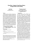
Having chosen the type of sensor, it was acquired the Current Transformer CR8349-1500
from CR Magnetics, Inc, shown in figure 3.2. This sensor is a general purpose vertical pcb
mount current transformer with small footprint. It’s main characteristics are:
• maximum current to be linearly sensed, Ir = 75 A;
• maximum saturation output voltage, Vmax = 12.8 Vrms ;
• frequency range 20 − 1KHz.
Figure 3.2: CR8349 Current Transformer
3.2.2
ADE7953 Theory of Operation
3.2.3
Data Acquisition System Deployment
Figure 3.3 represents a block diagram of the ADE7953 Evaluation Board in terms of
supplies and main inputs/outputs(I/O).
Power Supplies
As one may see in figure 3.3, the board has two separate power connections. The power in
the board is in two parts, one for the “hot part” where the analogue front-end is, and one for
the “cold part”, dedicated to communications. The reason for this isolation is the protection
19
VDD_COMM
VDD_AFE
Analog Frontend - HOT
POWER
GND_AFE
POWER
Ground Isolation
GND_COMM
SPI
I2C
UART
Communication - COLD
ADE7953
Signal
Conditioning
1000:1
Current
Channel A
IAP
IAN
Current
Channel B
IBP
IBN
Voltage
Channel
VP
VN
Figure 3.3: ADE7953 evaluation board I/O
of user and user-equipment connected to the communications interface, since that in the hotpart the ground may be coupled to high-voltage signals, due to the direct connection of the
system’s ground to one of the voltage’s inputs.
Both power inputs are rated to have an independent 3.3VDC ± 10% voltage supply[4].
The one connected to the hot part was based on a 3.3V regulator, a UA78M33 from Texas
Instruments, connected to the lab bench supply. The other one was deployed in conjunction
with the communication by a micro-controller development board connected to a PC, that
will be further discussed further ahead.
Voltage Sensing
The voltage sensing of the board can be directly driven by the utility’s voltage signal. The
VP input shall be driven with the Phase conductor, while the VN shall be driven with the
Neutral one.
This is done by connecting the conductors of the configurations power strip in parallel, as
depicted in figure 3.4, to the board.
Current Sensing
As mentioned before the ADE7953 Evaluation Board doesn’t provide a direct way to sense
current. One has to design sensory circuitry to allow current sensing, meeting the platform’s
20
UTILITY’S
POWER SOURCE
Phase
IAP
IAN
Current Transformer
CR8349
Neutral
VP
230 VRMS
VN
Figure 3.4: Load System Configuration
requirements.
Only one current channel needs to be used. Channel A was selected, since it is the most
versatile[4]. Current sensing will be then made through the current transformer mentioned
in subsubsection 3.2.1
The project of a transimpedance circuit to measure current is done in appendix C, where
the sensor circuit was deployed with a Rburden = 2.5Ω ± 1%. The circuit then connects to
the IAP and IAN of ADE7953 Evaluation Board.
3.3
3.3.1
Communicating with the Data Acquisition System
ADE7953 Communication Model/Memory Model
Before implementing any kind of communication with the ADE7953, it is important to
understand the underlying concepts. All of the features can be accessed through addressable
registers via 3 distinct communication interfaces.
Registers are 8, 16, 24 and 32 bit long. The data in 32 bit registers is the same of that
in its correspondent 24 bit registers, through signal extension. These differences are justified
with the 24 bit registers being more efficient in terms of communication speed while the 32 bit
registers provide easier programming with the long format [4]. All the registers are addressed
with a 2 byte value. The most significant byte (MSB) of the address contains an indication
of the register’s length, being the registers length equal to
register length = ((address’s MSB) + 1) × 8 bits .
(3.1)
The registers lengths and the corresponding address format are represented in table 3.3, where
X means don’t care.
21
Register Length
8 bit
16 bit
24 bit
32 bit
Address
0x0XX
0x1XX
0x2XX
0x3XX
Table 3.3: Register’s adressing scheme
The communication interfaces are three:
• 4 - pin SPI interface;
• 2 - pin bidirectional I2 C interface;
• 2 - pin UART interface [4].
Despite being carried out via different interfaces, the steps necessary to access the registers
are generically the same consisting in read or write one register at a time in an ask/reply
fashion. Figure 3.5 shows a minimal representation of a data transaction.
BUS
Command
R/W
Address
DATA
Figure 3.5: Minimal data transaction
3.3.2
ADE IO INTERFACE BOARD Z
To develop the system it is necessary to implement communication between the acquisition system and a PC. The ADE7953 Evaluation Board already comes with an interface to
communicate with a PC via USB, emulating a Virtual COMM. That interface is done with
a independent board, the ADE IO INTERFACE BOARD Z that connects to interface depicted in figure 3.3. This PC interface was developed to communicate directly to proprietary
software in LabVIEW, and allows to test the system with all the communication technologies allowed in the ADE7953, I2 C,SPI,UART [14]. But the protocol it uses to communicate
with the LabVIEW program is not available, nor the program’s API, making it impossible to
develop custom software around it.
It is then necessary to deploy another way of communicating with the acquisition system.
3.3.3
Communicating Directly
UART
Due to its simplicity, it was first tested the UART implementation, directly connecting
the PC to the ADE7953 through an USB-UART converter, that displayed in the PC as
virtual COMM. Though it was possible to establish communication, it didn’t provide enough
performance,it was limited to a 4800bps and the connection wasn’t reliable ,the culprit is it’s
22
timing scheme, that was not easy to guarantee by general purpose operative systems which
have scheduling granularity in the order of the of tens of milliseconds, while the protocol
has constraints in the order of milliseconds[4]. Posteriorly to this test, it was found one
configuration on the virtual comm driver that could have produced this behaviour, but another
solution with much better performance was already developed.
SPI
Since the UART interface did not meet the requirements, communicating via another
interface is imperative. The choice was SPI because it has the capability of being faster
in data transactions than I2 C. It can operate at a maximum clock of 5M Hz with one bit
per clock with an fixed overhead of 24bits per register access, while I2 C can operate at a
maximum clock of 400kHz with 1 bit per clock with an overhead of 16bits plus 1 start and
1 stop bit plus 1ack bit per byte written in the bus. Besides all that, SPI can be considered
simpler than I2 C.
3.4
SPI-PC Gateway Implementation
As normal PCs don’t provide external SPI interface. To fulfil the communications implementation, it is demanded to implement a gateway to provide the needed communication
interface. Some requirements are to be taken into account. The communication has to have
high bitrates, and should be compatible, i.e., should be in a connectivity interface present in
the majority of computers.
3.4.1
Chipkit Max32
Figure 3.6: chipKit Max32 development board [7]
Again, for fast integration, it was chosen to develop the gateway with an integrated solution, in this case a microcontroller development board. The platform chosen was chipKIT
Max32 by Digilent (figure 3.6), a microcontroller board based on Microchip PIC32MX795F512L.
For the project’s interest, this platform has the following features:
• PIC32 high performance 32-bit micro-controller at 80 M Hz with a 5 stage pipelined
MIPS core[35];
23
• Hardware SPI driver, performing with maximum of 40 M Hz clock[34];
• Hardware UART driver, with performance up to 20M bps[34];
• FTDI FT232R UART to serial UART that may perform at a maximum of 3 M baud at
7 or 8 bit symbols[7][16];
• 3.3V regulator that can provide up to 500 mA [7];
This platform meets all the connectivity and communications requirements. It exceeds
the SPI specifications of the ADE7953, it has USB connectivity in order to communicate with
a PC, that is good because that’s an interface that the majority of PCs have, and the UART
has high bitrates. Plus it is capable of supplying power to the communications interface of
the energy monitoring board, without any other connection than USB.
3.4.2
Gateway Deployment
Figure 3.7 presents a diagram of the gateway and its interface with the rest of the system.
3.3V
Regulator
5V
USB
COMM
USB to UART
FTDI232R
PIC32MX795F512L
SPI
UART-SPI
Translator
SPI
Processing Unit
MASTER
UART
SLAVE
I2C
UART
chipKit Max32
Analog and DSP Frontend
POWER
ADE7953
Communication
Interface
Figure 3.7: SPI gateway implementation
ADE7953’s SPI interface
ADE7953’s SPI interface is a fully functional SPI device that uses all four communication
pins. It operates in slave mode which means that a clock must be provided by the master.
This clock can be at maximum 5M Hz.
As said before, registers are accessed one at a time. The access to a register is encapsulated
in a SPI packet. Which is always initiated by the master, consisting in two initial bytes for
the register’s address. Then it is transmitted a command byte, to state if the access will be
a read or a write. Finally the data is sent from ADE7953 to the master in case of a read, or
written to ADE7953 by the master, in case of a write. All the data is sent or received MSb
first [4]. A representation of a packet may be found in figure 3.8.
24
Active BUS
Idle BUS
Idle BUS
15
0
0 7
Address
Address
31/23/15/7
Command
R/W
Command
Start of Packet
0
DATA
End of Packet
Figure 3.8: SPI Packet
PIC32 SPI Interface
The PIC32 provides a full function SPI hardware driver, that can provide master or slave
communications. For this implementation, this interface is configured as master, providing a
clock of 1 M hz to the slave and will be responsible of managing the communications. Assuming that the system needs the data from Voltage, Active Power and Reactive Power registers
at a frequency of 1.2kHz, being the registers of 24 bits and having the communications an
overhead of 24 bits, the minimum clock of the SPI has to be 173 kHz. This configuration is
more than sufficient to the specified requirements.
UART Interface
An UART interface is used to connect the gateway to a PC. This UART interface is
implemented with PIC32’s UART driver connected to FTDI FT232R USB-UART converter,
that connects with PC via USB, and is seen by Operative System (OS) as a virtual COMM
RS232 port. The interface is configured to operate asynchronously at a baudrate of 115200 bps.
Assuming that the gateway would work with an optimized protocol that sends to the PC the
needed data continuously with a minimum overhead of 2 bytes, one before the data and one
after, having the system to get data from three 24 bit registers at 1, 2kHz, the data has to
arrive at the PC at a rate of 48000bps. Being the UART configured at 115200bps, the actual
8
data rate is 10
× 115200 = 92160 bps, again the configuration is more than sufficient for the
specified requirements.
3.4.3
Communication Model
The communication model implemented in this gateway is coherent with the memory
model implemented in the ADE7953. The accesses are done to single registers, and issued via
the UART to the gateway. A write to a register is issued by sending a packet to the gateway,
with a write command, the address and the data to write. The gateway then is responsible
to communicate with the device, and forward the write transaction, as depicted in figure 3.9.
A read is issued by sending a read command with the register’s address to the gateway. Then
the gateway fetches the data, in the register, from the device and replies it via UART. A read
transaction is depicted in figure 3.10.
25
PC
Gateway
ADE7953
Write+Address+Data
Address+Write+Data
UART
SPI
Figure 3.9: Gateway Write
PC
Gateway
ADE7953
Read+Address
Address+Read
Data
Data
UART
SPI
Figure 3.10: Gateway Read
This communication model was chosen by its simplicity, and it is adequate for testing and
configuration purposes. However it has some limitations, namely it is not suitable for high
throughput systems that need synchronized data at very high sampling rate. Considering that
the PC-Gateway is much more slower than the Gateway-device, because of structural interface
26
limitations, the overhead introduced consumes valuable bus time that may jeopardize the
data synchronization, and that in other models could be used to send real data. Furthermore
issuing single access to registers introduces delays that are inconvenient.
A more suitable implementation would be such that, in case of read of registers could issue
repetitive reads of a list of register cycling through them. In case of the write of registers, it
could be also be improved by being able to write to several registers in a single access. Note
that writes aren’t critical since they are used almost only during the configuration phase of
the device, and in sporadic maintenance. Such a model would allow for the data to be read by
the PC at almost the maximum of the speed of the UART, by eliminating the overheads and
the round trip times, assuming that the Gateway-Device communication is much faster than
the PC-Gateway communication, which is usually true since the gateway is implemented to
a single purpose, being very efficient in one task, while the PC is designed to perform a high
number of tasks simultaneously, turning it mediocre in each task.
An example of an alternative method for high-performance access is represented in figure 3.11. A repetitive read is issued by a sending special command of cycle read and a list of
registers to read, the gateway than cycles the list repetitively by issuing reads in the ADE7953,
and when it has a new version of each register of the list it sends it to the PC via UART.
27
PC
Gateway
ADE7953
Read_Cycle+Addr1+Addr2
Addr1+R
Addr2+R
Data1
Addr1+R
Data2
Addr2+R
Data1
Data1+Data2
Addr1+R
Data2
Data1+Data2
UART
SPI
Figure 3.11: Gateway Read Alternative
28
3.4.4
UART Protocol
The UART protocol developed is based on the one for ADE7953’s own protocol for its
UART but without the time constraints [4]. A representation of a basic packet of the UART
protocol is represented in figure 3.12. A full description of the protocol implementation is
presented in appendix F.
Active BUS
Idle BUS
Idle BUS
7
0
0 15
Command
Address
Address
Command
0
7/15/23/31
DATA
Start of Packet
End of Packet
Figure 3.12: UART protocol basic packet
3.4.5
Gateway Firmware Model
Figure 3.13 presents the data-path/state machine inside the gateway, illustrating how the
operations are processed and how the communications are handled.
UART Message Handling
The handling of UART messages can be considered a process and flows as follows. A
start of a new message is detected after the Start of Frame Delimiter (SFD) has passed. The
type of message is then fetched. A decision upon what type of message is made. If a read
command is detected, the machine then fetches the next 2 bytes as address and finalizes the
message. If a write command was issued, the next 2 bytes are fetched, again, as address.
Next it is fetched the data, which length, here N_bytes, is found by analysis of the address’s
MSB, and finally the packet is finalized. The packet finalization depends also of the receiving
of End of Frame Delimiter (EFD). If any error is detected on SFD, EFD, or any other field
which data is different from what is supposed to, the program flow returns to the beginning,
with the start of a new message. After a message is finalized, the data is passed to the SPI
handling process
3.4.6
SPI Handling
SPI handling starts after a complete message is received via UART. Upon receiving, the
process decides what to do depending on the operation to perform. If a read was issued, the
system reads N_bytes ( again the length is found from the address) of the register, and sends
the read data out, via UART, and then finalizes the command. If a write was issued, N_bytes
of data coming from the data of the received packet, are written to the register, and then
command is finalized.
29
New Command
UART-Message
Handling
SPI
Handling
New
Message
Read
Fetch
Command
Read
Read/Write
N_bytes
Write
Fetch
Address
(2bytes)
Fetch
Address
(2bytes)
Fetch Data
(N_bytes)
Get Register
Size
N_bytes
New
Command
Read/Write
Read
N_bytes from
Address
Write
Write
N_bytes to
Address
Send
Register
Data
via UART
Finalize
Finalize
Figure 3.13: Gateway Dataflow
The system has ended the processing of a message and is ready to receive and process
another.
3.5
Wireless Sensor Network Nodes
The project’s proposition demands the deployment of a complementary WSN, to perform
Indirect Power Sensing of individual appliances, in order to augment the data available for
load disambiguation. These WSN has, too, some requirements. It has to cause the minimum
intrusion to customer’s space, has to be quick and easy to install, and preferably cheap. This
implies that the wireless sensor nodes need to be, small, battery-operated, and have to have
low power consumption for high autonomy.
3.5.1
uMRFs
The WSN nodes used were the the uMRFs, provided by Micro I/O Serviços de Electrónica, figure 3.14. They are developed for embedded solutions with wireless applications
and they satisfy the needed requirements. The nodes are compact and have small profile,
they are battery operated by a rechargeable Li-Ion battery. The processing capabilities are
provided by a 8-bit low power micro-controller from microchip, PIC18F26K20 with nanowatt
XLP. The wireless capabilities are provided by IEEE 802.15.4 compliant radio transceiver
MRF24J40MA, which protocol is designed for low power applications. They provide USB
30
Figure 3.14: uMRFs wireless node[5]
connectivity by a USB-UART converter. The USB connection can also be used to provide
power to the node and to recharge batteries[5].
The nodes provide direct digital input/output to the micro-controller via connection pins,
which will be used to interface to external sensors, sensing the environment[5].
3.6
Deployment of Indirect Power Sensing
The indirect sensing method is based on the fact that appliances may emit measurable
physical signals when consuming energy [21].
To indicate if some appliances are ON/OFF, according to the appliance model followed in
the project, it is necessary to implement sensory circuitry which output is directly correlated
with the appliance’s power state. Since there is no need to estimate the power consumption
from this, the circuits output was chosen to be digital, indicating only an ON or an OFF
state. The circuits developed were based on light sensors and magnetic sensors. Operation
and implementation details will follow.
3.6.1
Ambient Light Sensing Circuit
Lamps emit light when consuming power. Sensing the light intensity near a lamp is a way
to discriminate its internal state.
There exist such sensors called ambient light sensors. Ambient light sensors are photodetectors designed to perceive the power emitted in the visible spectrum. These sensors shall
be ideal for the end here demanded, as they can sense the most important output of a lamp,
which should be the easiest to detect.
There exist essentially two types of light sensors:
Light Dependant Resistors, CdS Cells - Commonly known as LDRs, these sensors vary
their impedance with the intensity of light, in a phenomena called photocondutance.
These sensors have Cadmium in its composition, not being suitable for consumer products having a RoHS prohibition.
Photo-diode/Photo-transistor - these detectors are semiconductor based, with p-n junctions that convert light in electricity, capturing photons, creating a photo current in
31
phenomena called photoelectric effect. The main difference between Photo-diodes and
Photo-transistors its the output/input gain, which is much greater in Photo-transistors
The selection of photo-transistor’s comes naturally, as they are RoHS compliant and are
easy to use.
The sensor used for light sensing was the TEPT5600 from Vishay, this is an ambient light
sensor based on a silicon NPN planar photo-transistor. It is sensitive to visible light much
like the human eye having its peak sensitivity at 570 nm[43].
The transistor is placed in a transparent case, capturing photons in the base-collector
junction, imposing a current flowing from collector to emitter,(photo-current).
Sensor Circuitry
The circuit to develop is a digital discriminator of presence of light, so it is wanted to
put the sensor in saturation. It’s then necessary develop a transimpedance circuit to convert
photo-current in voltage.This sensor circuit is to be attached to uMRFs where it will output
its digital value, and from where it will get its power supply of 3.3 V .
The circuit developed is presented in figure 3.15a, where it is represented the transimpedance circuit attached to a Schmitt-trigger, to output digital levels regarding the appliance’s state, ON or OFF. The design and analysis of the light sensor circuit is presented in
appendix D.
The sensor is designed to be placed near a lamp, where the light intensity is very high. A
final assembled version of the developed circuit/device can be seen in figure 3.15b.
to WSN
node
(a)
(b)
Figure 3.15: Light Sensor: a) - Light Sensor Circuit Schematic; b) - Assembled Sensor Circuitry
3.6.2
Magnetic Hall Effect Sensing
Proposition: one could measure/detect current flowing through a current carrying conductor by measuring the magnetic field around it, with a magnetic hall effect sensor.
Hall effect sensors are semiconductor based devices that when subjected to a magnetic
field, output a voltage proportional to the field strength [19].
32
Taking into account that this project aims to detect household appliances non-intrusively,
the place where one could place the sensor is attached to the electric cable of the appliance,
which generally is a two wire cable as represented in figure 3.16a.
From the Ampere’s Law, which an analysis is presented in appendix E, it was derived the
dependence of the magnetic flux at a distance r of the center of a fixed position two conductor
cable. The magnetic flux varies with the angle(θ) as expressed in equation 3.2. A normalized
plot of such equation is shown in figure 3.16b.
Iµ
Iµ
−
(T )
2πk(r cos(θ) − ri )x̂ + (r sen(θ))ŷk 2πk(r cos(θ) − (−ri ))x̂ + (r sen(θ))ŷk
(3.2)
The first term of the equation corresponds to the component of one of the conductors and it
is additive. The second term corresponds to the component of the other conductor and it is
subtractive because the current flow is in the inverse direction and so the field is symmetric
to the first.
B(θ) =
r
y
Ɵ
ri
x
(b)
(a)
Figure 3.16: Magnetic Flux around a two Conductor Cable: a) -Cut-section of a generic two
conductor cable; b) - Magnetic Flux vs Angle
From the plot, one can infer that the function maximum is obtained int θ ∈ {0o , 180o }
with the value
Iµ
Iµ
Bmax =
−
(T )
2π(r − ri ) 2π(r + ri )
and is minimum at θ ∈ {90, 270} with the value
Bmin = 0 (T )
since at that points the contribution of the magnetic flux of each conductor is equal in norm
but with inverse directions and so they cancel themselves.
If a hall effect sensor is to be attached to a power chord of an appliance, it should be possible to extract information about the current being carried in that conductor. This method
33
can be used to detect and measure the current flowing in the chord, but the uncertainty in
the cable placement and the possible sensor position drift, makes it only viable to detect if
the appliance is ON or OFF.
In conclusion, if one can find a sensor with sufficient sensitivity to sense magnetic fluxes
around a conductor and have special care with the sensor placement, it is possible to detect if
an appliance is consuming energy or not, and with sufficient training it could be even possible
to differentiate ON states, for multi-state appliances.
SS49E - Linear Hall-Effect Sensor IC
Figure 3.17: SS39 Series Linear Hall Effect Sensors[42]
The sensor selected was the SS49E Linear Hall-Effect Sensor IC, figure 3.17. This sensor
is a low cost and compact linear hall-effect sensor. The sensor aims to be used for basic
current sensing and for position/displacement sensing with a sensibility of 1, 4mV /Gauss[42].
Its main electrical characteristics are:
• Low voltage capability ranging from 2.7 to 6.5 V ;
• Analog Output with 1, 4 mV /Gauss sensibility;
• Maximum magnetic range of ±1000 Gauss;
• Wideband frequency response up to tens of kilohertz.
• Output voltage, Vout = 2.5 V at 0 Gauss
Detecting Appliance’s Power State
The objective is detecting the power state of the appliance by detecting the current flowing
in the cable. The aim is then to develop a circuit which output is a logical digital value
indicating the presence or not of current in a cable.
To perform the above mentioned function it is necessary to perform certain operations.
Figure 3.18 shows a simple diagram of the implemented circuit for indirect current sensing.
Further details of the development of this circuit are described in appendix G.
The output of the sensor, to our interest, is a sinusoidal wave at 50Hz with few millivolts
of amplitude.
34
SS49
Hall
Sensor
Band-Pass Filter
High-Pass Amplifier
Rectifier and Filter
Schmitt-Trigger
Figure 3.18: Block Diagram for indirect current sensing
The sensor’s output passes then through a band-pass filter to remove other frequencies
than that of interest. High frequency noise may appear due to radio signals.
The signal has very low amplitude, so it passes through an amplifier with high-pass
characteristic, in order to amplify the desired signal and reject any type of DC.
Being the signal at an amplitude in the order of the units of Volt, it is necessary to convert
it to a DC signal in order to further convert it to the digital signal. The signal is passed then
through a Rectifier and Filter that generates a DC voltage corresponding to the maximum
voltage of the Steady-State sinusoidal wave. In correct function the output here is a high dc
voltage when there’s current flowing in the cable, and null voltage otherwise.
The signal passes then through a Schmitt Trigger that converts the signal into a digital
value indicating the presence or not of current. It functions as a comparator with hysteresis.
A fully assembled version of the circuit can be seen in figure 3.19.
to Power
Supply
To WSN
node
Hall Sensor
Conditioning
Circuit
Figure 3.19: Fully Assembled Version of Indirect Current Sensor Circuit
3.7
Summary
This chapter presented the architecture solution and the hardware for the project.
The data acquisition system is based on ADE7953 Evalutation Board, a system that monitors an electricity facility, returning at high sampling rates various characteristics of the
electric circuit.
35
The communication between PC and data acquisition system is intermediated by a gateway that communicates with the PC via virtual COMM and to ADE7953 via SPI.
The indirect sensing WSN is deployed by uMRFs nodes, using PIC 8-bit micro-controllers
for processing and will communicate wirelessly via radio using IEEE 802.15.4 protocol.
Indirect Power Sensing is deployed by circuits attached to uMRFs. The sensors are be
based on photo-transistor for light sensing, and hall-effect sensors for current sensing. The
sensing is deployed in such a way that the circuits output digital values indicating ON or
OFF states.
36
Chapter 4
Software Implementation
4.1
Load Disambiguation and Appliance Classification
Before presenting the software solution for the Fine Grained Electricity Monitor it is important to acknowledge the underlying methods that will be in use. Following the NIALM
analysis presented in Chapter 2, it will be here described the main algorithm for load disambiguation and appliance classification, depicted in figure 4.1.
1.Data Aquisition
Measure Power and Voltage
RMS Data
2.Normalize
Normalized complex power
3.Step Detection
Step Changes
4.Appliance
Classification
Figure 4.1: Load Disambiguation Algorithm Representation
37
4.1.1
Initial considerations
To develop the algorithm it is necessary to choose the signature type that will be used to
detect the appliances, as well as their model.
The signature type used is the steady-state with nnormalized complex power, which is
tolerant to variations in voltage supply
The model in use will be the ON/OFF model , where each appliance has unique steady
state ON and OFF signatures, and where the OFF is the symmetric of the ON signature.
For identification purposes each appliance has a tolerance within its signature, which results
in the signatures being characterized by circles in the P-Q plane(in Phase-Quadrature, same
as Real-Imaginary) for each state. The circles must not overlap for any appliance signature.
4.1.2
Pseudo-code Implementation
In this subsection it is described the Load Disambiguation Algorithm in Pseudo-code to
complement the block diagram of figure 4.1
1
/∗ Data A c q u i s i t i o n and N o r m a l i z a t i o n ∗/
3
5
7
a t ( s a m p l i n g f r e q u e n c y Hz )
{
Vrms = g e t RMS V o l t a g e ( ) ;
Power = g e t Complex Power ( ) ;
Norm_Power = ( ( Nominal V o l t a g e ) / (V) ) ^2 ∗ Power ;
New_Norm_Power_Value ( Norm_Power )
9
11
}
13
/∗ S t e p D e t e c t i o n ∗/
15
/∗ S t e a d y S t a t e D e t e c t i o n ∗/
17
19
21
23
25
last_window_steady = f a l s e ;
a t ( s a m p l i n g f r e q u e n c y Hz )
{
power_window . push ( Norm_Power ) ;
i f ( power_window . STD < STD_Threshold )
i f ( last_window_steady == f a l s e )
{
/∗ New S t e a d y S t a t e D e t e c t e d ∗/
27
29
31
33
35
37
s t a t e . power=power_window . get_mean_Power ( ) ;
s t a t e . time = System . get_Time ( ) ;
new_Steady_State ( s t a t e ) ;
last_window_steady = true ;
}
else
{
power_is_changing ( ) ;
last_window_steady = f a l s e ;
}
38
39
}
/∗ S t e p C a l c u l a t i o n ∗/
41
43
45
47
49
51
53
55
f o r ( each new Steady S t a t e )
{
Step = ( o l d Steady S t a t e ) − ( new Steady S t a t e ) ;
new_Step_Detected ( Step ) ;
}
/∗ A p p l i a n c e C l a s s i f i c a t i o n ∗/
f o r ( each New Step D e t e c t e d )
{
/∗ Comparison by e u c l i d e a n d i s t a n c e ∗/
Closest_App_Signature = s t e p . f i n d _ c l o s e s t _ s i g n a t u r e ( ) ;
i f ( s t e p . i s _ w i t h i n _ t o l e r a n c e ( Closest_App_Signature )
{
/∗ A Change o f S t a t e i n an A p p l i a n c e has been d e t e c t e d ; ∗ /
57
A p p l i a n c e=Closest_App_Signature . g e t A p p l i a n c e ( ) ;
Event = Closest_App_Signature . getEvent ( ) ;
newEventDetected ( Appliance , S t a t e ) ;
59
61
}
else
{
No O p e r a t i o n ( ) ;
}
63
65
}
4.1.3
Data-acquisition
By sensing the installation’s current and voltage it is computed the RMS Voltage and
Power which are sampled for further processing.
4.1.4
Normalize
Normalize takes Voltage V and Power P as inputs and normalizes P through
Pnorm =
Vnom
V
2
P ,
(4.1)
where Vnom is the nominal voltage of the load being monitored. Following there is a pseudocode representation:
4.1.5
Step-Detector
The step-detector takes the normalized power as an input flow and sequences it into
changing periods and steady periods. The power values are inserted in a finite moving window
of length N . The operations of standard deviation and mean values are computed through
the window. A representation is shown in figure 4.2.
Standard deviation is used as a measure of how much the power is changing in the window.
If greater than the threshold STD-Threshold the power is considered to be changing at that
39
Normalized
Power
Window(N_Positions)
Standard
Deviation
Mean
Figure 4.2: Representation of the filter for step detection
moment. Once it goes below the threshold the power is considered to be steady. A timestamped sample of the mean power of the window is taken and registered as a steady-state.
The difference between steady-states is calculated and is considered to be a step. Not all
steps are to be considered because some of them may be too small, so they are compared to
a minimum threshold Step-Threshold. If greater, the step is registered and passed for further
processing, otherwise is discarded. Following there is a pseudo-code representation:
4.1.6
Appliance Classifier
Once a step is detected, it follows the identification of the appliance that changed state.
To achieve this goal, steps are compared with the signatures of the list of all known appliances
to find the closest one. Once the closest signature is found it is computed if it fits within
the appliance’s own tolerance. If it does it is registered a detection of an appliance change of
state, otherwise is discarded.
For illustration purposes, in figure 4.3 are represented detected steps and appliance signatures in the P-Q plane. Step-1 is detected, the closest signature is App2 ON. Step-1 is
contained in App2 ON tolerance, so Step-1 is classified as the Appliance 2 turning ON. Step2 ’s closest signature is App1 ON, but its not contained in the tolerance, so it is discarded.
This algorithm represents the basic operations needed to deploy, in order to provide
NIALM. However it isn’t supposed to provide a detailed solution for Load Monitoring, because it lacks appliance tracking, energy calculations and user interfaces. Following there is
a pseudo-code representation:
40
Detected Step-2
VAR
App1
ON
Detected Step-1
App2
ON
W
App2
OFF
App1
OFF
Figure 4.3: Steps and Signatures on the P-Q plane
4.2
Preliminary Validation of the Load Disambiguation Algorithm
Before implementing the system based on the algorithm presented, it is good practice
to assess if it can perform as it is supposed, i.e., if it provides a correct output, provided a
correct input.
4.2.1
REDD - A Public Data Set for Energy Disaggregation Research
Reference Energy Disaggregation Dataset (REDD) is a publicly available dataset containing detailed information on power usage from real household environments. It was created to
provide valuable data to research on energy disaggregation[22].
The data provided consists of whole home and device specific power consumption from
various houses over several months.
For each house it was recorded the whole home electricity signal at high frequency (15kHz).
For every recorded home the dataset provides data about up to 24 individual circuits. These
circuits are normally for categorized appliances. Data is provided at 0.5Hz. The dataset
also provides data about up to 20 individual appliances, that were monitored via plug-level
41
monitors. This data was recorded at 1Hz[22].
The only data that is useful in this project is that of the low frequency. In case of whole
home data, it is available the Real Power at a frequency of 1 Hz samples. In the case of
single appliance data it is provided again Real Power, but at 13 Hz. The sampling frequency
is different from the frequency it was recorded because it is the result of some processing and
not raw data.
For each monitored home there are individual files with data from aggregated load called
mains, and files for individual appliances.
4.2.2
Testing the Algorithm in MATLAB
The platform chosen to assess the algorithms validity was MATLAB, due to its flexibility
in programming and by making it easy to handle large quantities of data.
Single Appliance Characterization
A script that characterizes an appliance by executing the disambiguation algorithm upon
the data-flow of power of a single appliance was developed in MATLAB, and it performs the
algorithm as follows:
1 - Standard Deviation - The first step is pass the whole Real Power signal through
a finite length moving standard deviation. Figure 4.4 illustrates this step. In this case it was
passed a window of 4 samples through the data. As one can see the standard deviation signal
only rises when a step change in the power flow occurs, otherwise is steady near 0. This is
the first argument in favour of the algorithm.
2 - Steady State Identification - After passing the standard deviation, a threshold is
passed to its result to find where the signal is steady, and where the signal is changing. Once
the threshold is passed it is found the middle of the steady-periods, and taken a sample. That
sample is called a steady state. It is assumed that on the middle of a period the signal is
steady enough. Figure 4.5 shows the result of steady-state identification with the red bullets
indicating the middle of a steady state.
3 - Step Detection and Classification - Now that the steady-states are known it
is simple to calculate the step-changes. A differentiation of the consecutive steady-states is
performed, resulting in the step-changes. Not all step changes may qualify as steps of an
appliance as they may be too small. A threshold is passed through the step-changes in order
to eliminate false positives. Figure 4.6 represents the step identification. Positive steps( turn
ONs) are represented as represented in the middle of the steady-states as yellow-stems; and
the negative steps( turn OFFs) are represented as black stems.The step threshold used in this
case was of 100 W .
42
Figure 4.4: Pass of Standard Deviation window through the Real Power of an Oven
Figure 4.5: Representation of Steady State Identification
43
Figure 4.6: Representation of Step Identification
44
4.2.3
Results
Some of the appliance files of the REDD database were selected to validate the algorithm. After analysing the individual power flows of the various appliances it was possible to
characterize some. The parameters of the analysis were:
• Time interval: 3134061 seconds;
• Window Size: 30 seconds;
• Standard deviation threshold: 50 Watts;
• Step Threshold: 100 Watts.
Table 4.1 shows the results of the appliance characterization, Sig is the mean of the steps
detected, and STD is their standard deviation, Num events is the number of steps detected
for that state.
Appliance
Oven
Refrigerator
Dishwasher
Lighting
Microwave
Bathroom GFI
Washer Dryer
Sig(W )
1640
186
545
235
1524
1607
2706
Turn ON
STD(W ) Num Events
24
46
13
662
350
107
51
28
44
241
21
43
32
107
Sig(W )
−1639
−192
−452
−241
−1514
−1607
−2706
Turn OFF
STD(W ) Num Events
24
46
42
642
291
126
46
27
100
242
21
43
32
107
Table 4.1: Single Appliance Characterization of some appliances in REDD
Analysing the results one can verify that the algorithm is indeed capable of discriminating
step-like changes in well behaved power flows. Thus the standard deviation of the steps is
very low in the majority of the appliances detected. The OFF signatures are very close to the
symmetric of ON, apart from a small error, thus satisfying Zero Loop-Sum Constraint. And
the number of detections of ON states is coherent with the number of detections for OFF
states, satisfying in this way the Uniqueness Constraint described in section 2.3.
One of the appliances, the dishwasher, stands out having big Standard Deviation and
signatures very different in absolute and even not coherent in the number of detection. The
reason for this is that the appliance is not well described by the ON/OFF model for which
the algorithm was designed, because it is multi-state, being only possible to described by the
FSM model.
4.3
Preliminary Algorithm’s Software Implementation
Now that the algorithm was verified in MATLAB it is necessary to implement it in a
general purpose programming language. The programming language chosen was JAVA, for
its easiness integration and portability.
The implementation here is a bit different than that on Matlab, since the data is processed
iteratively as it is pushed into the processing, instead of being processed as a whole.
45
4.3.1
Step Detector
The heart of this implementation relies in the stepDetector class/interface, where are
implemented the structures and functions to perform step detection.
Firstly the structures:
Processing Window - This is the window for signal processing, where the power flow is
pushed to be analysed by the operations of standard deviation and mean.
Steady States Queue - This is a FIFO queue for steady-states, where they are pushed after
being identified. The data in this structure are states that are defined by a steady-state
power signature and a epoch time-stamp.
Non Steady-States Queue - Alongside the queue for steady-states there is a queue for
non-steady states which the only data of value to push in is the time-stamp of the
identification of a start of a changing period.
Steps Queue - This is the queue where the detected steps are pushed into, for passing to
further processing.
The methods:
Push into Window - This is a method to push one power sample to the window in order
to slide the power flow. Once the window is full, at each push the oldest sample is
discarded.
Steady Power Discrimination - This is a method to discriminate if the power in window
is steady, by comparing the standard deviation to a pre-determined STD Threshold.
States Identification - This is a method that by observing the succession of steadiness, or
not, of the power flow, identifies and pushes a steady-state, a power sample with the
mean of the window at the time of the detection and the time-stamp, to the Steady-State
Queue. The non steady-states are also identified and pushed to the Non Steady-State
Queue with a dummy power sample and the time stamp.
Step Detection - This is a method that takes at each time the two least recent steady-states
and finds the distance between them comparing it to a step-threshold, and classifying
if they are steps, pushing a power sample of the difference between the steps and a
time-stamp for that sample.
4.3.2
Preliminary Appliance Classifier
Having the steps been identified, another important part of the system is the appliance
classifier. For that there is another class/interface implemented, that is responsible by identifying the appliances that are turning ON and OFF, given the step changes.
There is an Appliance structure for registering what appliances are in the system, in
which the classifier relies to perform the classification. In a preliminary implementation this
structure has the parameters:
• Name - The name of the appliance;
46
• ON Signature - Complex power Steady-State Signature of the ON state;
• OFF Signature - Complex power Steady-State Signature of the OFF state;
• State - Flag indicating if the appliance is ON or OFF ;
There is also a database where the data about all the appliances is stored, in order to be
further accessed.
The classification starts with the computing of the minimum euclidean distance between
a given step to every signature of all the appliances in the database, with the goal of identifying
the closest signature and consequently the appliance and the event, an ON or an OFF, that is
candidate to have occurred. The identification ends by the verification if the step is contained
within a predetermined tolerance. If so, the step is classified with the event and the appliance.
The state data of the appliance in the database is also updated.
4.3.3
Process data-flow
Having the methods and structures been defined, it can now explained the processing flow
of the data.
The power samples are pushed into the window. Next, the steady power discriminator
takes the standard deviation and the mean from the window, and discriminates the steadystates from the non steady-states. After the discrimination the step identification is made
taking into account the consecutive steady states. The steps are then taken into appliance
classification, where the appliances being turned ON or OFF are identified and the database
is updated. Summarizing the dataflow must pass through this steps in order:
1. Steady State Discrimination
2. Step Identification
3. Appliance Classification
4.3.4
Validation
With the software implementation defined it is necessary to assess its accuracy and correctness. For this it was taken the aggregated load of some data from REDD and the characterization of some appliances from table 4.1, and it was performed load disambiguation in
order to find the Refrigerator and Oven appliances. The parameters used for the process
were:
•
•
•
•
Window - 15 seconds for single appliance, 5 seconds for mains data ;
Standard Deviation Threshold - 5 W ;
Step Threshold - 25 W ;
Fixed Appliance Tolerance - 40 W ;
The results presented are from the first 800000 seconds of the records. Table 4.2 compares
the number of detections made by detection of appliance in single appliance file, with detection
of appliances in the aggregated load in the mains file, by the algorithm implemented in Java.
47
Power
Window(N_Positions)
Standard Deviation
Mean
Non Steady-States Queue
Steady-States Queue
State1
State1
Steady Power
Discrimitation
State2
State3
State2
State3
State4
State4
...
...
Step
Identification
Steps Queue
Step1
Step2
Step3
Step4
...
Appliance
Classification
Appliance and Event
Appliance Database
Figure 4.7: Preliminary Implementation of the NILM system
Appliance
Oven
Refrigerator
Single Appliance
ON
OFF
13
13
173
179
Mains
ON OFF
17
20
165
128
Table 4.2: Comparison of detection in single appliance files to detection in aggregated load
mains file
Analysing table 4.2 one can see that the number of ON/OFF events detected are close
but not equal. These errors arise from the low sampling frequencies on the power flows and
the big number of appliances on the mains file. That two characteristics result in overlapping
events that are seen as noise by the system, causing the miss of detections of some events.
Figure 4.8 represents identification of appliances in the mains file by the JAVA routine, the
power flow of total load and the power flows of individual loads. In figure 4.8a it is represented
the identification of a refrigerator in the total load. The refrigerator is identified well even
when there are other appliance events happening along the function of the refrigerator, but it
is also seen a false identification caused by a signature very close to that of the refrigerator.
In figure 4.8b it is represented the identification of an oven. The same observations made for
48
(a)
(b)
(c)
Figure 4.8: Appliance Identification in mains aggregated load: a) - Refrigerator Detection;
b) - Oven Detection; c) - Refrigerator and Oven Detection
refrigerator apply in this case, although here it is shown a miss of an identification caused by
the events that are very close, due to low sampling frequency. In figure 4.8c it is represented
the simultaneous detection of refrigerator and oven. From the figures here presented and the
49
data in table 4.2 it’s established the correctness of the suggested algorithm. It is important,
now, to develop the infrastructures and interfaces to apply the algorithm to real data acquired
by the data acquisition system, and to develop a full functioning Monitoring system.
4.4
Fine Grained Electricity Monitor
With the proposed algorithm verified it is now opportune to develop the Fine Grained
Electricity Monitor. The system developed can be decomposed in various logical entities,
which are represented in figure 4.9
Indirect Power
Sensing WSN
Data
Acquisition
Data Logging
Step Detection
Statistics and
Calculations
Appliance
Classification
Graphical
User Interface
(GUI)
Fine Grained Electricity Monitor
Figure 4.9: Fine Grained Electricity Monitor and its logical entities
Data Acquisition - Obtains raw data and manipulates it to normalized power;
Step Detection - Takes normalized power and identifies steps within it;
Appliance Classification - From identified steps classifies it in meaningful appliance events;
Data Logging - Records and saves any data valuable for processing and statistics;
Statistics and Calculations - Takes historical and real time data to produce meaningful
statistics and figures;
Graphical User Interface - Shows real-time data and historical statistics about power consumption in order to deliver valuable data to the user;
Indirect Power Sensing WSN - Provides individual state data about appliances of interest, to help in disambiguation of similar loads;
In the center of the system there is a logical database which holds all the valuable data
for the systems function, where all the data, either externally fetched or internally computed
or, is stored.
50
4.4.1
Data Acquisition
Data Acquisition
Data Acquisition
System
VRMS
Raw Data
Convertion
IRMS
Normalized
Power
DATABASE
Recorded Data
Power
Figure 4.10: Data Acquisition Logical Entity
The data acquisition entity, depicted in figure 4.10, is responsible of communicating with
the data acquisition system already described. Its basic function is to read and write registers
from the ADE7953. The data in the registers doesn’t have a direct physical meaning, thus
it is considered to be raw data. So this part of the system is also accountable for converting
raw data into meaningful physical values, i.e. Volts, Amperes, Watts, Watt Hour etc.
The data acquisition layer obtains repeatedly at a frequency of 50 Hz the following values:
• VRM S - RMS Voltage;
• IRM S - RMS Current;
• P - Complex Power, it is composed by two values: active power and reactive power;
The values of VRM S and P are used to compute a sample of normalized power at the same
frequency as of that of the sampling of those values. Alternatively to the sampling of the
values of power consumption from the data-acquisition system, there is also the possibility of
providing the system with data recorded previously by the system, by the data-logging entity.
All the obtained and computed values are timestamped and pushed into the database.
4.4.2
Step-Detection
The Step-Detection entity, depicted in figure 4.11, takes the samples of normalized power
from the logical database, and sequences the flow in steady-periods and changing-periods. Then
identifies step-change events in the power-flow, that are the difference of the average power of
consecutive steady-periods intercalated with changing periods. The steps are identified by its
characteristic value of Power and its time-stamp of occurrence. The steps are then pushed
to the database. No further discussion on this aspect is needed since this subject has already
been thoroughly discussed.
51
Step
Detection
DATABASE
Normalized Power
Flow
Steps Queue
Step1
Step2
Step3
Step4
...
Figure 4.11: Step-Detection entity
4.4.3
Appliance Classification
Although appliance classification has been already discussed, in concept and implementation, the implementation that will be here presented is different from the one previously
exposed.
Before presenting the actual implementation of the algorithm it is important to present
some concepts on the database that are necessary for the appliance disambiguation.
Appliance Database
The system here developed only identifies appliances known a priori. This means that
the all appliances passive of being detected must be first identified and catalogued with their
characterization. Therefore it was implemented in the database an appliance database in
which all the appliances of interest must be described, in order to provide sufficient data for
appliance detection and tracking of operating state. An entry of the appliance database has
the following parameters:
• Name - Name of the appliance for identification;
• ON Signature - Complex power-steady state signature of ON state;
• OFF Signature - Complex power-steady state signature of OFF state;
• Tolerance - Scalar value of tolerance in for identification of steady-state signatures;
• State - Indicator of the appliance’s current state, ON or OFF ;
• Sensor Address - Physical address of the node monitoring the appliance. This parameter will only exist for the appliances monitored via Indirect Power Sensing WSN,
and will be explained later.
52
Appliance Classification Process
A step is fetched from logical database and then compared with all signatures of all appliances in the appliance database. Once the closest signature, by euclidean distance, is found,
it is assessed if it is contained within the appliance’s signature tolerance, as in figure 4.3. If
so, it is then checked if the event is coherent with the appliance’s current state, since a turn
ON can’t occur if the appliance is already ON neither a turn OFF if the appliance is already
OFF. Provided that all the information is consistent, the appliance state is updated, and the
detection of an appliance event is signalized in the database. The appliances monitored by
Indirect Power Sensing WSN are discarded from this process. This process is illustrated in
figure 4.12
Steps Queue
Step1
Step1 Fetch
Step2
Step3
...
Appliances’
Signatures
Data Consistency
Check
DATABASE
Appliance
Comparison
Name: Heater
ON: 1000W
OFF: -1000W
Tolerance: 5%
State: OFF
Update
Database Update
Appliance Database
Update
Appliance State
Appliance Database
Appliance Event
Signal
Appliance
Event
Figure 4.12: Appliance Classification Process
4.4.4
Data Logging
Despite the system being designed for real-time monitoring, not all data expected to be
produced is real time data. Historical data for statistics and other calculations are of the
highest importance. There is also interest in improving the system, by the development of
more sophisticated algorithms.
To satisfy these requirements it was developed a Data Logging module that records the
data that may be of interest to further experiences and processing. Figure 4.13 represents
53
the data-logging entity. The entities recorded in the database are:
• Data Acquisition - VRM S , IRM S and Normalized Power;
• Step Detection - steady-states and steps;
• Appliance Classification - events associated with every appliance individually in
separate files and all appliances together in a single file;
• Estimated Power - the power resulting from the sum of power being spent by all the
appliances detected to be ON ;
Indirect Power
Sensing WSN
Data
Acquisition
Step Detection
Appliance
Classification
VRMS
IRMS
Power
Sensors Events
Steady States
Steps
DATABASE
• Indirect Power Sensing WSN - all the detected changes of state of the monitored
appliances.
Data Logging
Appliance
Detections/Events
Figure 4.13: Data-logging entity
4.4.5
Indirect Power Sensing WSN
The Indirect Power Sensing WSN is a Wireless Sensor Network designed to monitor
individual appliances and provide its internal power state to the Monitor. It is demanded to
be easy to configure and have low power consumption.
The network was developed with the following principles in mind:
Star Topology - There is one master node responsible for network maintenance and coordination;
Self Configuration - The network configures itself when deployed, favouring easiness of
installation;
54
Event Driven Communication - The network tends to communicate only when there is
new information on the nodes, using minimum energy when not in function;
An in depth analysis of the WSN development and operation is documented in the report
of the project “Monitoring System [17]” developed in the course of Redes de Comunicação
em Ambiente Industrial( Communication Networks in Industrial Environment).
Network Topology
The network is deployed in a logical star topology with a master node in the center,
connected to a PC, and the slaves attached to the appliances to monitor. Communication
only occurs between master and slaves.
Network Self Configuration
The network configures it self at start-up. The slave requests the master for registering in
the network and awaits for reply. The master receives the request, acknowledges the presence
of the slave in the network, and sends a reply to the slave indicating that it has been registered.
Once the slave receives the reply of the registering phase, its is ready to work normally.
Network Maintenance
The network has detection of failures, for slaves, by an “I’m Alive” mechanism. This
detection of failures mechanism is implemented by the imposition on the slaves of a periodical
transmission to the master(an “I’m Alive” message), to indicate that it is working. The master
detects if there is any problem with a slave, by detecting failure in receiving the “I’m Alive”
messages from the slave.
WSN System Function
The master is in the center of the network. It has full knowledge of all the slaves in
the network, as well as the states of the sensors monitoring the appliances. The master is
responsible for coordinating the network, and to communicate with the PC informing it of
all the states of sensors and signalize when a state change occurs in any of the appliances.
The slaves are at the ends of the network and attached to the appliances being monitored.
The slaves must inform the master every time their sensors detect a state change in an
appliance.
In figure 4.14 it is represented the network and a sequence of events that occur when one
appliance changes state. Slave 1 detects a state change in the appliance that it monitors,
and informs the master of that occurrence. After checking the information’s coherency, the
master informs the PC of the change of state in the sensor.
55
Change
detected
Slave1
Slave1
State Change
Slave2
MASTER
Slave1's
Appliance
has changed state.
Slave3
Figure 4.14: WSN Representation
4.4.6
WSN entity
Before describing the WSN entity function specificities, it is necessary to present some
concepts about the abstraction here developed. The WSN monitors individual appliances
with sensors, that are used to infer the internal power state of the appliance. To that matter
there is a Sensor Database inside the WSN entity that holds information about the individual
sensors present in the WSN. The entries of the database have the following parameters:
• Sensor Address - Physical address of the WSN node;
• Status - State of the sensor. It can be ON indicating the attached appliance is on,
OFF indicating that the appliance attached is off, or Disconnected indicating that the
WSN node is malfunctioning.
The WSN entity role can be seen as two different tasks. The WSN Interface, that is
responsible for communicating directly with the network, retrieves information about the
sensors. The WSN Classifier/Tracker is responsible by treating the state changes on the
sensors and relate them with the changes in the appliance database. These tasks are linked
in the access to the Sensor Database. Figure 4.15 illustrates the WSN entity architecture.
WSN Interface
The WSN interface is responsible for managing the communications between the WSN
and the Electricity Monitor. This interface provides an abstraction layer that is agnostic with
respect to the network, the Indirect Power Sensing WSN is seen as a simple data device.
56
Sensor Changed
State
Indirect Power
Sensing
WSN
WSN Interface
Update Sensor
DB
Sensor Addr: 10
State:ON
Sensor Database
Appliances’
Sensors’ Adresses
Sensor Event
Find Address
WSN Classifier/
Tracker
DATABASE
Signalize Event
Name: Heater
ON: 1000W
OFF: -1000W
Tolerance: 5%
Update
Update
State: OFF
Appliance Database
Appliance State Sensor: 10
Appliance Database
Appliance Event
Signal
Appliance
Event
Figure 4.15: Indirect Power Sensing WSN entity representation
Thus it provides a notification mechanism that fires, asynchronously, notifications every
time a state change is detected in any sensor. Additionally, it also permits the access to
information about the sensors available and their status, by request.
At start-up the interface builds the sensor database with all the sensors and their current
state. Then, at normal operation, it waits for messages from the WSN with information
about state changes on sensors. Once a message about a change in a sensor is received, it is
checked if the change is allowed, taking into account the current state of the sensor. If so,
the information on the database is updated and a notification for the WSN classifier with
the information about the occurrence of state change on a sensor is fired.
WSN Classifier
The WSN Classifier waits for an event notification on state change of a sensor. Then, by
the Sensor address, it fetches the correspondent appliance from the Appliance Database. It
checks if the announced change is valid. If so, the appliance entry in the Appliance Database
is updated, and a notification is fired in the Logical Database signalizing an appliance state
change event.
57
4.4.7
Statistics and Calculations
Having power consumption and times of state changes for every appliance available, it
is possible to compute some very interesting statistics. Those may be Energy Spent/Cost
by appliance, variation of power consumption by time of day/weekday/weekend, duration of
time each state is visited etc.
None of this statistics are currently computed, but with the data provided by the logging
system it could be achieved with minimum effort.
Nonetheless there are some calculations made by the system. The system computes the
estimated power, that is the sum of the characteristic power of the appliances that are on
the ON state at each moment. Recalling from boolean switch process a(t) of equation 2.1 the
estimated power, Pestimated , is:
Pestimated (t) =
N
X
Pi ai (t) ,
(4.2)
i=1
where Pi is the power consumed by the ith appliance when in ON state.
Another calculation made is the residual power, Presidual , which is the difference between
the total measured power and the estimated power, which is analogous to e(t) in equation 2.2
and can be interpreted as a measure of completeness and accuracy of the system[18].
Presidual = PT otal − Pestimated .
4.4.8
(4.3)
Graphical User Interface
The Graphical User Interface(GUI) is designed to provide to the user all the system’s data
of interest, being it real time and historical.
The GUI is connected to the database, fetching the the following data about the electric
circuit in:
• RMS Voltage;
• RMS Current;
• Normalized Complex Power in active and reactive components.
It also fetches the following the computed real time data:
• Expected Power, in the active and reactive components;
• Residual Power, in active and reactive components.
The GUI should also fetch the historical and the computed statistics data, but that isn’t
implemented and should be considered for short term future work. Apart from that, the GUI
listens for the events of the appliances changing states, as well as it fetches information about
the appliance database. A representation of the data transactions of the GUI is represented
in figure 4.16.
58
VRMS
IRMS
Complex Power
Circuit
RT DATA
Estimated Power Calculations
Residual Power
GUI
Appliances’:Name
State
Signatures
Appliance Database
Appliance
Changing State
Appliance
Events
Figure 4.16: Graphical User Interface entity
Figure 4.17 represents the default aspect of the GUI. The GUI is divided in two tabs.
The Graphs tab is oriented to display the data about the electric installation and plotting the
graphs of interest. The Apps tab displays the data about the appliances in the circuit.
Graphs Tab
The graphs tab shows real time traces of RMS Voltage and RMS Current, as can be seen
in figure 4.18.
It is also shown real time traces of the components of power. As it can be seen in figure 4.19,
both the measured total power( blue trace) and the estimated power( red trace) are present.
All the traces are updated at 50 Hz.
59
Figure 4.17: Graphical User Interface default appearance
Figure 4.18: Graphics with traces of RMS Voltage and RMS Current
Figure 4.19: Graphics with traces of the components of complex power of Total Power and
Estimated Power
60
In parallel with the graphs, it is also displayed some information in text form about the
electric installation and about the events that are happening in the appliances. As shown in
figure 4.20 it is displayed the values of:
• VRM S - RMS Voltage;
• IRM S - RMS Current.
• Complex power components in the measured total power, and in estimated power.
There is also a field called Events that is updated at the detection of an appliance event and
flashes, so it can get the user’s attention. Under that field there is also a scrolling list of the
last 10 events that have happened, appended to their time-stamp.
Figure 4.20: Informations about the electrical installation
Apps Tab
The Apps Tab was designed to provide visual information about the appliances. Not only
the current state but some historical data and other calculations should be displayed. But
in the current implementation it only shows the appliances in the system and their detected
states. Figure 4.21 shows the Apps Tab in operation. As one may see, there are three types
of states for appliances. ON and OFF are self explanatory. The Undetermined state is
the default for the appliances at start-up. Since the appliances states are detected at their
changes, if no state change is detected one should not infer the appliance’s state, although it
may be possible for special cases, such as no power being drawn which means all appliances
are OFF, their state is left Undetermined.
61
One feature that was projected to have but is missing is that, when clicked on any of
the appliances, historical statistics and data on appliances power consumption, such as the
times of operation and the energy cost of its usage, was to be shown. This feature should be
considered for future short-term implementation.
Figure 4.21: Apps Tab of Graphical User Interface
4.5
Summary
In this chapter it was presented the algorithms and structures for a Fine Grained Electricity
Monitoring system. The algorithms were tested and validated. This led to a preliminary
implementation in software that was also tested and validated.
The algorithm’s preliminary implementation in software was the basis for the development
of the system’s implementation.
The implementation consists in:
• Data Acquisition;
• Appliance Classification;
• Indirect Power Sensing WSN;
• Statistics and Calculations;
• Data Logging;
• Graphical User Interface.
To the Indirect Power Sensing WSN it was seen that it is self configurable, and that it
integrates with the PC like a data-device. Thus it notifies the system about the changes of
state in individual appliances.
62
In terms of inputs/outputs the system gets RMS Voltage, RMS Current and Complex
Power from the Data Acquisition System and gets individual states of some appliances from
the Indirect Power Sensing WSN. It produces as output appliance disambiguation, calculations and statistics on historical data and logging of all data of interest.
Finally it was presented the Graphical User Interface(GUI), the ultimate output for user’s
feedback. It shows real-time data on the electric installation( VRM S , IRM S , Power) and the
calculated Expected Power. On the appliances side the GUI shows the appliances present in
the circuit as well as their operating state.
Statistics and calculations on historical data are not yet implemented. But the data logger
already records data in a way that make the future implementation very easy.
63
64
Chapter 5
Tests, Results, Validations and
Calibrations
This chapter presents a set of tests that have been carried out to validate the system. In
addition it is also presented the calibration methodology.
5.1
Test-bed
Taking into account that the system should monitor a household electrical installation, it
was developed a test-bed that simulates the electric circuit of a house.
The electrical power source is taken from a standard 230 VRM S power outlet to a 6 outlets
power strip. The voltage signal is directly fed to the data acquisition system through a connection in parallel with the power strip, while the current signal is fed to the data acquisition
system through a current transformer in the phase conductor of the power strip. Figure 5.1
shows the most important components of the test-bed’s electrical installation.
Along with the electrical installation it is deployed the WSN based Indirect Power Sensing
that aims at disambiguating similar appliances. There are sensor nodes with light sensors,to
monitor 2 equal lamps,which cannot be disambiguated solely by the normal algorithm. It is
also deployed one sensor node with a magnetic sensor coupled to a fan heater. The reasons for
this are that it showed to have a rather slow transient, what made the detection through load
disambiguation difficult, while the detection through indirect power sensing WSN showed to
be more reliable.
Connected to the data-acquisition system and to the Indirect Power Sensing WSN there
is a PC, which executes the all necessary tasks to perform the Electricity Monitoring.
65
UTILITY’S
POWER SOURCE
Phase
IP
DATA
Acquisition
System
IN
Current
Transformer
FAN
RADIATOR
LAMP
Neutral
VP
230 VRMS
VN
(a)
FAN
LAMP
Power
Strip
Data Acquisition
System
Analog Interface
FAN
Heater
(b)
Figure 5.1: System’s electric installation testbed: a) - block diagram, b) - physical instalation
66
5.2
Calibration
Calibration is very important in systems that depend on measurements and sensing of
environment quantities. Furthermore, from the nature of load monitoring system, that aims
to be an energy meter, it is expected that it is a device with great accuracy and correctness,
so that it meets or exceeds the common household revenue meter.
The main measurement system is the ADE7953 - Evaluation Board, in which the measures
of Voltage and Current need to be calibrated. To calibrate a system one needs references.
The reference used for voltage measurement was Fluke 287 True RMS Multimeter, while for
current measurement the reference used was Tektronix A622 AC/DC Current Probe connected
to a Tektronix TDS 210 Oscilloscope.
5.2.1
Calibration of Measurement System
ADE7953 ADC Gain error Calibration
The gain error is defined as the per-channel difference between the ADC output code and
the ideal output code. Thus ADE7953 provides gain error calibration for each of its ADC
channels. The gain adjustment allowed is in the range of [0.5; 1.5]. The gain adjustment is
set in appropriate registers and is regulated by equation 5.1.
Output = Input ×
GAIN
,
0x400000
(5.1)
with 0x200000 ≤ GAIN ≤ 0x600000.
The gain error calibration for voltage and current channels can be performed using the
values of VRMS and IRMS from the registers of ADE7953 and with the measurements of
RMS voltage at ADC’s channels’ input. Knowing that the ADC has a full scale input of
500mV and that the expected value in the registers of VRMS and IRMS at full scale input,
500
√ mVRM S , is 9032007d[4], the calibration equation becomes
2
GAIN = 0x400000 ×
Value Expected
,
Value Actual
(5.2)
which can be modified, in order to be applied iteratively, to
GAINi = GAINi−1 ×
Value Expectedi
,
Value Actuali
(5.3)
with i the order of the iteration. The first iteration assumes GAINi−1 = 0x400000.
The calibration method for any of the ADC channels is:
1. Get VRMS or IRMS registers from ADE7953 during an interval of 10 seconds at a
sampling frequency of 10Hz. Compute the mean value to get Value Actuali . Parallelly,
measure the mean value of VRM S at ADC’s channel input with multimeter during the
same 10 seconds interval, with that value find Value Expectedi ;
2. Apply equation 5.3 to calculate GAINi ;
3. Apply GAINi to the system;
67
4. Repeat step 1 and check current accuracy;
The calibration method is to be repeated for any of the channels until one gets the desired
accuracy.
Checking Voltage Channel Accuracy
Let Vmeasured be the mean value of RMS voltage at the data acquisition’s voltage input
measured in 10 seconds intervals. Let Vactual be the mean value of samples of the VRMS
register taken at 10Hz during the same interval.
Knowing that between the Voltage input of the data acquisition system and the ADE7953 ’s
voltage ADC channel is a 1 : 1000 voltage divider, it is easy to compute the voltage at the
ADC’s input, disregarding any error in the voltage divider which should be very small. It is
possible to compute the value that was expected in the VRMS register, namely Vexpected , that
is
√
2
Vexpected = Vmeasured ×
× 9032007 .
(5.4)
500
Thus the gain error is
Vexpected
.
(5.5)
errorgain = 1 −
Vactual
The Fluke 287 True RMS multimeter’s accuracy is
accuracy = ±([% of reading] + [number of least significant digits]).
(5.6)
For the range of the measurements used, which was 500V AC for a signal at 50Hz is
accuracy = ±([3% of reading] + [25 × 0.01V ])
(5.7)
Table 5.1 shows the results of the assessment of the gain error, comparing it to the accuracy
of the reference. errorgain represents the ratio in percentage of the gain error of the ADC to
Vactual and accuracy represents the accuracy of reference multimeter regarding Vmeasured . It
may be observed that the gain error is always smaller than the reference’s accuracy, which
means that the calibration may exceed the reference’s performance, therefore it is not possible
to improve the calibration with this reference.
Vmeasured [V ]
211.05
213.93
218.70
219.13
221.93
224.60
225.36
227.96
228.24
Vexpected [LSB]
5391562
5465136
5586992
5597977
5669507
5737716
5757131
5823551
5830704
Vactual [LSB]
5412301
5483521
5617941
5617941
5689227
5768089
5777579
5845952
5849892
errorgain [%]
0.38
0.34
0.39
0.36
0.35
0.53
0.35
0.38
0.33
accuracy[%]
0.42
0.42
0.41
0.41
0.41
0.41
0.41
0.41
0.41
Table 5.1: Assertion of gain error following the calibration of voltage channel
68
Checking Current Channel Accuracy
Let Ivmeasured be the mean value of RMS voltage at the ADE7953 ’s current ADC channel
input measured in 10 seconds intervals. Let Iactual be the mean value of samples of the IRMS
register taken at 10Hz during the same interval.
Following the same principles as those on the ADC’s voltage channel. Iexpected is the
expected value at the IRMS register for Ivmeasured and is computed as
√
2
Iexpected = Ivmeasured ×
× 9032007 ,
(5.8)
500 × 10−3
and so the gain error is
errorgain = 1 −
Iexpected
.
Iactual
(5.9)
The range of measurement used in the multimeter was 50mV AC with a signal of 50Hz.
The accuracy is
accuracy = ±([0.3% of reading] + [25 × 0.001mV ])
(5.10)
Table 5.2 shows the results of the assessment of the gain error comparing it to the accuracy
of the reference. errorgain represents the ratio in percentage of the gain error of the ADC to
Iactual and accuracy represents the accuracy of reference multimeter regarding Ivmeasured . It
may be observed that the gain error is always smaller than the reference’s accuracy, which
means that the calibration may exceed the reference’s performance. Once again it is not
possible to improve the calibration with this reference.
Ivmeasured [mV ]
5.326
5.328
5.350
12.702
12.777
Iexpected [LSB]
136060
136111
136673
324490
326406
Iactual [LSB]
135535
135618
136792
325841
326448
errorgain [%]
-0.39
-0.36
+0.09
+0.41
+0.01
accuracy[%]
0.77
0.77
0.77
0.50
0.50
Table 5.2: Assertion of gain error following the calibration of current channel
RMS Voltage and RMS Current Meter Constants
The data obtained from ADE7953 registers doesn’t have direct physical meaning, as it
is relative only to the values sampled in the ADCs. Thus it is necessary to convert the raw
values into meaningful values in Volts, Amperes, Watts, etc.. These values that convert the
register data to physical values are called Meter Constants. All the values needed to the
project, that are related to the electrical installation are related RMS Voltage and Current,
so it is only necessary to find Meter Constants for these. The others can be subsequently
derived.
These relationships may be expressed as
Vconstant =
Current Input [V ]
Voltage Input [V ]
, Iconstant =
VRMS [LSBs]
IRMS [LSBs]
69
(5.11)
The meter constants ought to be calculated under Steady conditions and with very precise
loads. It was observed that voltage varies with the load in the circuit. In addition the testbed is connected to the installation of a large building where numerous appliances are always
working and switching, so one cannot guarantee the steadiness of voltage. For this reason a
simple measure of VRM S or IRM S does not suffice to accurately find the meter constants.
The meter constants will be computed with the linear regression of various points of
current and voltage observed with different loads.
Method of calibration for Voltage Meter Constant
A list of ordered pairs {VRMS[LSBs], Voltage Input[V ]}, Voltages List, needs to be obtained by the following steps:
1. Set System’s load;
2. Get VRMS register from ADE7953 during an interval of 10 seconds at a sampling frequency of 10Hz. From the values obtained compute the mean to get one VRMS[LSBs]
value. Parallelly, measure mean value of VRM S at the Electric Installation input with
the multimeter during the same 10 seconds interval to get one value of Voltage Input[V ];
3. Store ordered pair in Voltages List;
The previous steps are to be repeated until the needed number of values are obtained.
Next a linear regression of Voltage Input[V ]/VRMS[LSBs] must be made to get the
Voltage Meter Constant.
The linear regression result was a voltage meter constant of
VmeterConstant = 3.887799914 × 10−5 [VRM S /LSB ]
(5.12)
with a correlation factor
R2 = 0.9995
(5.13)
b = 0.6726 VRM S
(5.14)
the offset was
that represents an error of errorof f set ≈ 0.3% which is very small and lower than the reference
meter’s accuracy. For being so small, and for system’s simplicity, this error was not taken
into account.
Table 5.3 compares the value of RMS voltage at the utility’s electrical installation measured by the reference multimeter, VRM S , with the measurements by the data acquisition
system, VRM Sactual . The error of the data acquisition system in relation with the reference
measurements is lower than the provided accuracy and is mainly due to the discarding of
offset on the calibration.
Method of calibration for Current Meter Constant
A list of ordered pairs {IRMS[LSBs], Current Input[A]}, Currents List, needs to be obtained by the following steps:
1. Set System’s load;
70
VRM S [V ]
211.05
213.93
218.70
219.13
221.93
224.60
225.36
227.96
228.24
VRM Sactual [V ]
210.42
213.19
218.06
218.41
221.19
224.25
224.62
227.28
227.43
errorM constant [%]
0.30
0.35
0.29
0.33
0.34
0.16
0.33
0.30
0.35
accuracy[%]
0.42
0.42
0.41
0.41
0.41
0.41
0.41
0.41
0.41
Table 5.3: Results of the voltage meter constant fitting
2. Get IRMS register from ADE7953 during an interval of 10 seconds at a sampling frequency of 10Hz. From the values obtained compute a the mean to get one IRMS[LSBs]
value. Parallelly, measure IRM S , at the phase cable of the Electric installation with the
current probe attached to an Tektronix TDS210 Oscilloscope to get Current Input[A]. It
was not possible to measure accurately the mean current in the interval, so the current
input is taken as a sample of instant peak current, which, is then transformed into a
RMS value.
3. Store ordered pair in Currents List;
The previous steps are to be repeated until the needed number of values are obtained.
Next a linear regression of Current Input[A]/IRMS[LSBs] must be made to get the Current Meter Constant.
The linear regression result was a current meter constant of
ImeterConstant = 2.392182902 × 10−5 [ARM S /LSB ]
(5.15)
with a correlation factor
R2 = 0.9998
(5.16)
b = −0.0219 ARM S
(5.17)
the offset was
The accuracy of the Tektronix A622 AC/DC current probe at the scale measured, that
was 100mV /A, is
accuracyprobe = (3% of measurment) + (50 mA).
(5.18)
The accuracy of the Tektronix TDS210 oscilloscope on the function used, that was Delta
Volts, is
accuracyosciloscope = (3% of reading) + (0.05 div).
(5.19)
Table 5.4 shows a comparison between the current measured by the current probe and
the oscilloscope, IRM S , with the current measured in the data-aquisition system when scaled
by the current meter constant IRM Sactual . One can see the accurate fitting of the values
from the data- acquisition system, with the error, errorM constant , always smaller than the
measurements’ accuracy, accuracy. This means the system meets the accuracy of the reference
and that discarding the offset in the scaling of the values is not significant.
71
IRM S [A]
0.188
3.230
7.920
IRM Sactual[A]
0.182
3.299
7.922
errorM constant [%]
-3.42
2.14
0.04
accuracy[%]
29.82
5.14
4.78
Table 5.4: Results of the current meter constant fitting
5.2.2
Calibration of Sensors in Indirect Power Sensing WSN
Because the nodes in the Indirect Power Sensing WSN perform measurements, it is also
necessary to guarantee that they produce the correct outputs to the designated inputs. To
this matter it is necessary to calibrate them in site to check its proper function.
Light Sensor Nodes Calibration
The sensor should be placed near the lamp to be monitored. An example of a correct
placement is shown in figure 5.2.
Figure 5.2: Light Sensor Placement
Calibration Method
1. Place sensor node;
2. Turn the Lamp ON ;
3. Check if sensor’s output reflects Lamp’s state. If not:
• Tune potentiometer on board until the sensor’s output is correct;
4. Turn the Lamp OFF ;
5. Check if sensor’s output reflects Lamp’s state. If not:
72
• Tune potentiometer on board until the sensor’s output is correct;
This method is to be repeated until the sensor node outputs the correct information about
the Lamp’s state;
Magnetic Sensor Nodes Calibration
The sensor placement requires it to be very close to the supplying cable. Figure 5.3 shows
an example of correct placement of the magnetic sensor, in which the sensor is in direct touch
with the cable and strapped with a nylon clamp.
Figure 5.3: Placement of magnetic sensor
Calibration Method
1. Tune potentiometer on board to approximately mid position;
2. Attach sensor to the cable of the appliance to be monitored, and supply it;
3. Turn the appliance ON ;
4. Install oscilloscope probe on the output of the second amplifier;
5. Rotate sensor around the cable and find the position where the signal has maximum
amplitude;
6. Fix sensor position;
7. Check signal’s amplitude, tune potentiometer until the amplifier outputs a signal with
amplitude close to 3V , in order to put the system in saturation, to guarantee correct
operation;
8. Check sensor’s digital output and verify if it is stable, and if reflects appliance’s state.
If not:
73
• Some tuning in the potentiometer may be needed;
9. Turn the appliance OFF ;
10. Check sensor’s digital output and verify if it is stable, and if reflects appliance’s state.
If not:
• Some tuning in the potentiometer may be needed;
This method is to be repeated until the results are satisfactory.
5.3
Appliance Characterization
Before presenting the results and tests to the system it will be presented the appliance
characterization. This is done here to justify the values of power detected in the system while
testing its accuracy and validity.
The appliances were characterized by steady-state and by turn ON and turn OFF transients in normalized power consumption, recorded by the acquisition system at a sampling
frequency of 50Hz for approximately 10 seconds.
The steady-state signature was found by taking one sample of the power consumption of the
appliance after approximately 10 seconds of being turned ON on a cold start, assuming that
all the transients are over after that period. The rise time is the time that the appliance’s
power consumption takes to rise from 1% to 99% of the steady state signature after being
turned ON. The fall time is the time that the appliance’s power consumption takes to fall
from 99% to 1% of the steady state signature after being turned OFF.
The appliances available in the test-bed are:
• Two-Level Radiator Heater - this appliance is categorized in two appliances Heater1
and Heater2, since the system is incapable of treating multi-state appliances.
• Two 100W Lamps - These lamps were specifically introduced for having 2 identical
appliances in the system, in order to exploit the problem of identification of similar loads
with the Indirect Power Sensing WSN. Only one will be characterized, it is assumed
that the other to be equal.
• Desk Fan
• Fan Heater
the characterization of the appliances is summarized table 5.5.
Appliance
Heater1
Heater2
Fan
Lamp
Fan Heater
Signature(W )
806.75 − 21.32i
1210.49 − 30.31i
39.78 − 0.80i
106.62 − 4.72i
1030.64 − 5.60i
Rise Time(s)
0.14
0.14
8.46
0.22
1.56
Fall Time (s)
0.16
0.16
6.11
0.18
0.18
Table 5.5: Appliance’s Characterization
74
Analysing the results from table 5.5, it is clear that the appliances that should be mainly
resistive, such as the radiator heater and the lamp, have faster transients than those that
have inductive element and high mechanical inertia, have slower transients, such as the fan
heater and the fan. Furthermore, the values obtained for the rise and fall times for the fan
are much higher than the others. This comes from the fact that it is a very small load in
which its transient may be confused with noise present in the system. The reactive power
measurements of the system seem to be disconnected from reality by a systematic error that
is shifting them negatively. However, this error does not affect the detection of loads, as the
algorithm only requires that the signatures are separated in the P-Q space;
5.4
5.4.1
Testing the Load Disambiguation Algorithm
Step-Detector
For testing the step-detector, step-like waveforms were introduced to the system by switching ON and OFF the appliances in the test-bed, and analysing the step-detector output, which
is provided by the data-logging entity, and is characterized by a time-stamp and a steady-state
signature in complex power.
Here it is tested the ability of the system to detect steps of the different appliances
individually.
For each appliance a test was performed, by turning ON the system, and introducing
a sequence of 21 consecutive switches with a period of approximately 4 seconds between
switches, to let the power stabilize. The step-detector parameters used were window_size =
10, step_threshold = 25 W and ST D_T hreshold = 5W .
In the results of the test, it was analysed the deviation of the detections from the steadystate signature, as well as the number of detections. Table 5.6 presents the results of these
tests. For each appliance tested Nr Detections is the number of steps detected, Mean Deviation
is the mean of the deviations from the steps detected to the steady-state signature with Value
being the norm of the Mean Deviation and Ratio, the ratio between the mean deviation and
the appliance’s signature. Max Deviation represents the maximum deviation detected. Value
and Ratio values have the same meanings as stated before.
Appliance
Heater1
Heater2
Fan
Fan Heater
Lamp
Nr Detections
21
21
21
21
21
Mean Deviation
V alue[W ] Ratio[%]
3.09
0.38
3.78
0.31
6.95
17.48
28.26
2.74
0.46
0.43
Max Deviation
V alue[W ] Ratio[%]
4.41
0.54
6.02
0.49
9.35
23.49
32.52
3.15
1.39
1.30
Table 5.6: Results of Single Appliance tests on step-detector
From table 5.6, it can be concluded that all the steps were detected for all the appliances,
which can be interpreted as a measure of correctness of the step detector.
Due to the nature of the system it is necessary to detect the appliances in real-time, thus
the system cannot delay its processing in order to wait that the transients of the appliances
to end. There is, so, an inherent notion of the signal being sufficiently stable to be detected as
75
a steady-state. This notion is expressed by the detection of steady-state upon a threshold on
the standard- deviation of the processing window. This can affect the step-detection in a way
that the steps detected may not be exactly equal to the appliances steady-state consumption,
though they shall be close.
The appliances that should be mainly resistive, such as the radiator heater and the lamp,
have very fast transients and the detections are very close to the steady-state signature, being
the most straight forward to detect.
Appliances that by nature of the physical task present slow transients, such as the fan
and the fan heater, which have motors that require long times to stabilize the spinning speed,
present greater deviations from steady-state signature. Another effect worth to notice in
this type of appliances is that the detected signatures may differ greatly if a turn ON is
performed by cold start, i.e. the motor is stopped, where the transient will be the slowest
and the deviation will be big, or if a turn ON is performed briefly after a turn OFF while the
motor is still spinning, where it can be observed that the detected step deviation is almost as
small as those of the resistive loads.
From the above discussion it follows immediately that a certain amount of time must
elapse between the occurrence a state change and the identification of the appliance that
experienced that change. This latency is defined as the detection time.
It was verified that the step-detector also performs well when there are various sources of
steps in the system and even when the steady state of the system is not null. The conclusions
are the same of those of when the system is tested with single appliances.
The Analysis of the deviation from steady-state signatures will allow the existence of a
starting point in defining the tolerances for appliance detection in the Appliance Classifier
5.4.2
Appliance Classifier
The appliances were catalogued in the Appliance Classifier with the steady-state signatures
from table 5.5 and with tolerances with the immediate unit upper-bound in percentage of the
maximum deviation as described in table 5.6.
It was found that some of the appliances were not being detected correctly in the total
load. For this reason the tolerances were tuned in order that all the appliances were identified
and correctly classified, taking into account that none of the intervals corresponding to the
signatures would overlap. The tolerances were tuned to those on table 5.7,
Appliance
Heater1
Heater2
Fan
Fan Heater
Lamp
T olerance[%]
5
5
25
5
5
Table 5.7: Appliance classification tolerances
In figure 5.4 is represented the classification of the appliances in the complex power plane.
The ellipses limit the intervals where the appliances are detected while the dots represent the
scatter of the identification of the appliances.
Figures 5.5 and 5.6 show a scatter of detections of the appliances within their tolerances.
76
Big loads, such as the Radiator Heater(Heater1 and Heater2) and the Fan Heater, show
small scatters, being well defined within their intervals. The Fan heater seems to have a larger
scatter, which is mainly due to the effects of the motor.
Small loads, such as the Lamps and the Fan, have greater scatters since they are more
prone to the inherent errors of the system and load variation. The Fan seems to have the
greater scatter. This may be caused by being the smallest load detected, and also because of
the effects of the slow transient of its motor. Moreover, the effect of switching the appliance
ON in cold start or while the motor is still spinning seems to have a very relevant effect.
Fan Heater-OFF
Heater2 ON
Heater1-ON
Lamp-OFF
Fan-ON
Fan-OFF
Lamp-ON
Heater1-OFF
Heater2-OFF
Fan Heater-ON
Figure 5.4: Appliance Classification in I-Q plane
77
Figure 5.5: Appliances’ Individual Interval of identification - a
78
Figure 5.6: Appliances’ Individual Interval of identification - b
5.4.3
Indirect Power Sensing WSN
The WSN is monitoring two lamps by light sensors and the fan heater with a hall sensor.
When put to function it was observed that the WSN detected almost all performed events.
It was not possible to characterize the detection accuracy, due to lack of time for thorough
tests.
5.4.4
Simultaneous detection of appliances
The system was configured to try to identify the loads simultaneously by the WSN and
by the Load Disambiguation Algorithm. It was found that the WSN only failed to detect the
lamps’ events 1 time out of 54 events that were introduced in the test. More, the WSN hasn’t
failed to detect the Fan heater in a test of 60 events.
From the data obtained it was possible to compute the relative delay between the the
detection of the events on the load disambiguation algorithm and the detection on the WSN.
In the following the detection by the load disambiguation algorithm is being used as the time
reference. Figure 5.7 shows histograms of the delay in bins of 50ms. From the figure, it can be
concluded that the most common delay in Lamp detections is in the interval of [200; 250[ms,
while the most common delay for Fan heater detections is in the interval of [100; 150[ms.
From the results in figure 5.7 and from table 5.8 and from the fact that the WSN detection
79
Figure 5.7: Histograms of the delay between the detection by the WSN and by the loaddisambiguation algorithm
Appliance
Lamp
Fan heater
Min[ms]
-220
-325
ON
Mean[ms]
+97
+1
Max[ms]
+265
+160
Min[ms]
-240
-240
OFF
Mean[ms]
+131
+57
Max[ms]
+300
+180
Table 5.8: Analysis of the delay in the WSN detection
only failed once in the realized tests, it can be inferred that the Indirect Power Sensing WSN
is reliable in detection of the desired events, and has a performance that is comparable to
the appliance detection in the Non-Intrusive Load technique. It can be concluded that the
the detecting of appliances via WSN does not compromise the accuracy and correctness of
the system, and can be used as true detector for single appliances without the requirement
of correlating information about the power of the electrical installation.
80
5.5
Complete System Test and Validation
To verify the correctness and accuracy of the developed system, it was simulated the
function of a home environment with all the appliances switching ON and OFF independently
from one another.
The system was set-up to detect the Fan and the Two-level radiator by the load disambiguation algorithm and the 2 Lamps and the Fan heater individually by the Indirect Power
Sensing WSN
A sequence of 100 switch events was performed by switching ON and OFF the appliances.
To avoid introducing dependence upon switching, events were performed following a random
sequence of numbers from random.org[37] website. The periodicity of the switches was 30
seconds to guarantee that the power is steady, thus it is expected that all the transients are
over, and to be physically possible by manual operation.
The following data was collected:
• Measured Power;
• Expected Power;
• Residual Power;
• Events detected for each Appliance;
Table 5.9 presents the events performed and those which were detected by the system.
Appliance
Heater1
Heater2
Fan
Lamp1
Lamp2
Fan heater
Performed
Turn ONs Turn OFFs
9
9
5
5
8
8
8
7
8
8
13
12
Detected
Turn ONs Turn OFFs
10
10
5
5
5
5
9
8
12
12
13
12
Table 5.9: Detection of appliances in a random sequence of events
The two level Heater Radiator has shown to be the most easy and straightforward load to
detect, being detected correctly all the times in the test. The extra detections denoted in the
table were due to human error during the execution of the sequence of events. The Fan is not
one of the best appliances to detect via NIALM because it is very small and any noise and
variations on the load have great impact in its correct detection. Thus it was noted during
the tests that every time that the Fan was switched ON after the Fan heater was switched
ON the system would fail to detect the fan. It is believed that this behaviour is due to the
slow transients of the fan heater, and it is affecting the detection of the Fan, preventing its
step from being detected. The Lamps were noted to be detected well by the WSN during the
tests. The extra detections noted in the table were due to some cross-talk between lamps, and
also between the environment, due to non optimal conditions. The Fan heater was detected
correctly by the WSN.
81
From the Measured Power, Estimated Power, and the Residual Power, one can verify the
accuracy of the system by characterizing the quality of the estimation. Figure 5.8 shows plots
of the above referred power flows. From figure 5.8 it can be seen that Estimated Power follows
Figure 5.8: Comparison of Measured Power with Estimated Power
the Measured Power very closely. The Residual Power is most of the time close to zero.The
peaks are due to the delay on the detection.
A characterization of the error of the system can be quantified by the norm of the Residual
Power, compared with the Measured Power.
Value
Norm of Measured Power
Norm of Estimated Power
Norm of Residual Power
Mean[V A]
1306.44
1305.96
20.91
Standard Deviation[V A]
834.61
836.84
96.15
Table 5.10: Comparison of Norms of Power Values
From table 5.10 it can be seen that the Measured Power and the Estimated Power values
are very close and consequently the Residual Power value is low.
Knowing the values of power, it is straightforward to get the values of energy by integration. Table 5.11 shows the energy of the different power flows.
Value
Measured Energy
Estimated Energy
Residual Energy
Energy[J]
3883990.521 -63343.642 i
3882473.341 -68701.747 i
1515.048 +5358.200 i
Energy[kW h]
1.078886 -0.017595 i
1.078465 -0.019084 i
0.000421 +0.001488 i
Table 5.11: Energy Values by integration of Power Flows
82
The values of Measured Energy and Estimated Energy are very close and consequently
the Residual Energy is low. In terms of absolute ratio the Residual Energy is 0.143% of the
Measured Energy. This value is the error of the system. This result is very good as a measure
of the completeness and accuracy of the developed system.
5.6
Summary
This chapter addressed the evaluation of the system’s correctness and accuracy. It started
by presenting the test-bed that would allow the system’s test and its calibration. Tests were
performed on some individual components of the system, the Step-Detector, the Appliance
Classifier and the Indirect Power Sensing WSN, which results have shown their correct implementation. To finalize, the system was tested as a whole and results were presented in
order to provide indicators of completeness and correct function. It has been verified that the
system detects the appliances with great success, and that the mean error on the energy by
integration of power was 0.143%.
83
84
Chapter 6
Conclusions and Future Work
6.1
Conclusions
A system capable of monitoring a household electrical installation was successfully implemented. The system disambiguates and identifies individual appliance loads within the
aggregated load, recurring to NIALM techniques.
The problem with identifying electrically identical loads was successfully tackled with the
Indirect Power Sensing WSN. It was shown that it was possible to detect the internal power
state of some appliances by using simple sensors that sense physical quantities in the vicinity
of the appliances. It was possible to detect lamps with light-sensors placed near the luminous
source. It was also possible to detect large loads by sensing the magnetic field created by the
current flux in their supply cable with a hall-effect sensor attached to it, without the need of
breaking the circuit.
The gathered information is used to find the state of the appliances in the circuit, being
able to tell what appliances are ON or OFF in real time, and historically. This information
is believed to be useful for improving the user’s awareness of how he is spending electrical
energy, and hopefully for providing insight to reduce his consumption habits in order to reduce
the expenditure.
The overall cost of the data-acquisition system system is low. Although the ADE7953
Eval-Board was expensive, its cost doesn’t reflect the material value, and it can be made very
cheap. Thus, considering the availability of small, low-cost computers such as the Raspberry
Pi, in my opinion a system like the one here developed , even if without the Indirect Power
Sensing module, could be very easily deployed in every home, without a representing big cost
to the costumer, and it would pay itself in short term, if the user would be willing to change
its consuming habits, based on the report on the consumption of the domestic appliances.
For more advanced monitoring and appliance classification/disambiguation, the Indirect
Power Sensing WSN can be also deployed at a relatively low-cost. It is, however, less costeffective mainly because of the cost of the wireless nodes components, namely the micro
controller and the radio-interface and batteries. Thus the sensors used are inexpensive, and
present nearly no cost footprint to the system.
Nevertheless, the system here developed is far from being a commercial system ready
to be manufactured. Further research on Appliance Models and automation of Appliance
Cataloguing and Naming is needed to provide the end user an easy to use and deploy system,
with minimal set-up effort and calibrations.
85
6.2
Future Work
Concerning future work there are plenty of ways one can improve the system to perform
better and provide more valuable information, in terms of either end consumer data or data
that enables more sophisticated appliance disambiguation and classification.
Thus there are certain objectives that are to be deployed immediately and others that
may be delayed to further implementation.
The most immediate need is the deployment of an improved communications interface, as
stated in Section 3.4.3 of Chapter 3, in order to enable higher data throughput.
There may arise the need for improving the appliance model in order to support multi-state
appliances, as there are already various examples of such appliances in any home. That solution would pass through implementation of an appliance model based on finite state machines
as suggested in Nonintrusive appliance load monitoring[18].
As the appliance pool rises there may be the need of deployment of other techniques for
appliance identification, so it’s proposed augmenting the appliance detection with transient
analysis, as documented in Power signature analysis[24], harmonic signatures as suggested
in Nonintrusive appliance load monitoring[18] and probabilistic and stochastic analysis of
appliance’s usage as in Circuit-Level Load Monitoring for Household Energy Management[28].
To account with the augmented parameters for appliance detection and identification there
could be implemented Artificial Neural Networks with the previously mentioned data as inputs, that through sophisticated functions and self-learning could output the states of the
appliances in the system, as documented in Real-Time Recognition and Profiling of Appliances
through a Single Electricity Sensor[38].
One aspect of the current system that needs to be improved is the use of the computed
data to produce valuable statistics on energy consumption, such as detailed electrical bill
discriminating the appliance’s cost, intervals of consumption, variance of consumption on a
time-basis or temperature-basis etc.. That may be one of the easiest parts to implement and
one of the most important features for a finalized product.
Other features that may have to be considered concern the automation of the system,
in order to make it easy to use and install. This could be implemented by building a large
database of appliances were the deployed system would go and look for signatures for the
features it has found. This database would be on-line, to allow remote access and would grow
with data gathered by user’s experiences, as in the RECAP system[38].
86
Appendices
87
Appendix A
Available Electric Monitoring
Integrated Solutions
Here it is presented a market survey of the most adequate solutions of integrated systems
on electrical energy monitoring.
A.1
Analog Devices - ADE7953
The ADE7953 is a high accuracy electrical energy measurement IC intended for single
phase applications. Analog Devices sells it a single IC, and has also an Evaluation board for
consumers to evaluate its performance. In the following sub-subsections we present the main
features of these platforms.
Figure A.1: ADE7953 functional block diagram [4]
89
A.1.1
ADE7953 - Single Phase, Multifunction Metering IC with Neutral
Current Measurement
The ADE7953,functional block diagram presented in figure A.1. It has one voltage channel and two current channels, and measures line voltage and current and calculates active,
reactive, apparent energy over programmable periods, plus is capable of waveform sampling
in over a 1.23 kHz bandwidth in the measurements:
• Vrms
• Irms
• Active Power
• Reactive Power
• Power Factor
The IC measures some power-line figures with voltage sag detection and period measurement, no load detection and zero crossing detection is also provided.
A variety of current sensors are supported, such as are Rogowski Coil Sensors, current
transformers or low value shunt resistors, due to its PGAs and Integrators in the current
channel path.
All ADE7953 features can be accessed via a three different communication interfaces:
• 4-pin SPI interface
• 2-pin bidirectional I2C interface
• 2-pin UART interface
[4]
A.1.2
ADE7953 – Evaluation Board
The ADE7953 evaluation kit includes two boards that together allow the performance of
the ADE7953 single phase energy metering IC to be evaluated, (ADE7953 Interface Board
and ADE7953 Evaluation Board)
• The interface board handles the communication from PC to the ADE7953.
• The Evaluation board includes the ADE7953, the needed isolation for high voltage
inputs and anti-aliasing filters( figure A.2).
All features available in the ADE7953 are available through supplied software, or directly
using SPI, I2C or UART communication [14].
90
Figure A.2: ADE7953 Evaluation board [14]
A.2
A.2.1
Microchip’s MCP3909
MCP3909 Energy Metering IC with SPI Interface and Active Power
Pulse Output
The MCP3909 is an energy-metering IC designed for standard metering applications, the
functional block diagram is presented in figure A.3. Its architecture is based on two 16bit second order delta-sigma Analog-to-Digital Converters( ADCs) and it has Programmable
Gain Amplifiers in order to allow different types of current sensors.
The IC is capable of making waveform measurements and output them digitally via SPI.
The IC is capable of waveform sampling Current and Voltage over a bandwidth of 14kHz
and output the digital data via SPI [30].
Figure A.3: MPC3909 Functional block diagram [30]
91
A.2.2
Microchip’s MCP3909/dsPIC33F 3-Phase Meter Reference Design
Microchip supplies various energy-metering designs for evaluating MCP3909’s performance, being the Microchip’s MCP3909/dsPIC33F 3-Phase Meter Reference Design the most
interesting to this project.
The Microchip’s MCP3909/dsPIC33F 3-Phase Meter Reference Design is a energy-meter
with many advanced features( figure A.4). It’s based on the MCP3909 for waveform sampling
of power line and dsPIC33F for signal processing and calculations. The current sensing is
done by current transformers.
Figure A.4: MCP3909/dsPIC33F 3-Phase Meter Reference Design [29]
This meter is ready for 3-phase metering with neutral current and it produces the following
data for each of 3-phases and to its total:
• line frequency
• Vrms
• Irms
• real power
• reactive power
• power factor
• fundamental active power
• fundamental reactive power
• harmonic component measurement for voltage from the 2nd to the 31st harmonic
92
• harmonic component measurement for current from the 2nd to the 31st harmonic
Each of these measurements and calculations are based on frequency analysis( DFT based)
are updated every 3 line cycles and accessible via UART, which can provide, at it’s best, a
sampling frequency of 16 Hz of the desired parameters [29].
A.3
Maxim’s 78M6613
A.3.1
78M6613 Single-Phase AC Power Measurment IC
The 78M6613 is a single phase AC power measurement IC designed for simplified metering
of power supplies and smart appliances.
Its architecture is based in four analogue input channels, a 22-bit sigma-delta ADC, a 32bit dedicated Computational Engine for calculations and a programmable 80515 at 5MIPS
for memory access, SFR control and communications. It has digital I/O ports for interfacing
with other devices, with its functional block depicted in figure A.5.
With appropriate firmware the IC is capable of the following measurements:
• Vrms
• Irms
• apparent power
• real power
• reactive power
• phase angle
• power factor
• line frequency
The communications are done via UART, with a maximum baud-rate of 38.4 kbit/s [2].
A.3.2
78M6613 Evaluation Boards
Maxim provides two evaluation boards to assess 78M6613 performance:
78M6613 - EVM - Evaluation Board - figure A.6a, is a system designed to perform measurements up to two single AC loads. The current sensing is done by current resistor
shunt and the communication is made via USB emulating a serial port. The measurement capabilities are the same as the single IC [1].
78M6613SP - EVM - Split Phase Evaluation Board - figure A.6b, is a system designed
to perform measurements to a single electrical outlet. The system provides two independent phases measurement, since in the US each outlet has two 120Vrms phases and
one neutral. The current sensing is done through current transformers and the communication is made via USB emulating a serial port. The measurement capabilities are
the same as the single IC [3].
93
Figure A.5: 78M6613 Functional block diagram[2]
94
(b)
(a) 78M6613 - EVM - Evaluation Board[1]
Figure A.6: 78M6613 Evaluation Boards:(a)78M6613 - EVM - Evaluation Board[1],
(b)78M6613SP - EVM - Split Phase Evaluation Board[3]
95
A.4
Continental Control Systems - WattNode ModBus
WattNode ModBus is a kilowatt energy and power meter designed to monitor up to three
phases. A schematic of the WattNode connected to one phase is represented in figure A.7.
Figure A.7: WattNode connection schematic [44]
It provides for each phase and for the total load the following measurements:
• Vrms
• Irms
• true RMS power
• reactive power
• power factor
• true RMS energy
• line frequency
This measurements are updated at every second via EIA RS-485 with ModBus. The
current sensing is done by Current Transformers [44].
A.5
Microchip’s PIC18F87J72 Single-Phase Energy Meter Energy Monitoring PICtail Plus Daughter Board
Microchip’s Energy Monitoring PICtail Plus Daughter Board is a low cost power monitor
based on the PIC18F87J72 single chip as the energy meter IC(figure A.8). Being a low cost
design the current sensors are shunt resistors. The system relies on the microcontroller’s
16-bit sigma-delta ADCs, and in its computational in order to do the measurements:
• Vrms
• Irms
• active power
• reactive power
96
Figure A.8: Microchip’s PIC18F87J72 Energy Monitoring PICtail[33]
• active energy
• reactive energy
• line frequency
The measurements are available at every line period, corresponding to a 50 Hz sampling
frequency, via USB, emulating a serial port [13] [33].
97
98
Appendix B
Current Sensing Technologies
Survey
In the current days the most used technologies in current measurement are low resistance
current shunts, current transformers, Rogowski coils and Hall effect based current sensors. In
this section it is presented a survey of the main characteristics of each solution, in order to
choose the most adequate.
B.1
Low Resistance Current Shunts
Current shunts are the most cheap and simple solution to measure current. They can be
accurately modelled by a series connection of a low resistance shunt and a parasitic inductance
with the load, with the total current to be measured passing through it, being its output
described by the transfer function of equation B.1,
+
Lsh
Il
Rsh
−
Figure B.1: Current shunt simple model
V = Rsh Il + jωLsh Il ,
(B.1)
It must be taken into account when designing the sensor, a phase mismatch due to the
parasitic inductance.
As there is no galvanic isolation of the hot parts of the circuit the shunts are normally
used in low, ground referenced currents in the order of the tenths of Amperes[32]. It must be
99
also noted that these kind of sensors dissipate high amounts of power which cause the need
for thermal dissipation, increasing the sensor’s footprint and cost.
Figure B.2 shows some examples of shunt resistors.
Figure B.2: Examples of Current Shunt Resistors[9]
B.2
Current Transformer
One of the most used and most reliable solution for measuring current is using current
transformers. These rely on the transformer’s magnetic coupling between two coils, being the
primary provided by the user, being commonly only one turn. A simple model of a current
transformer is shown on figure B.3. And the input/output current relation is represented by
i2
i1
n1
n2
Figure B.3: Simple model of a Current Transformer
equation B.2,
n1
i2
=
,
n2
i1
(B.2)
i1
,
n2
(B.3)
that can be generalized to equation B.3.
i2 =
The number of turns on the secondary must then be designed to suit the application’s need.
As one may see, this sensor provides galvanic isolation, making it safe for measuring high
currents. This solution is very precise over a wide range of frequencies, up to hundreds of
kilohertz but it suffers of the problem of not being able of measure nor admit DC due to
saturation of the magnetic core. Also current transformers can introduce phase shift and
special care should be taken to compensate this error.
Considering power, one can say that it consumes little power compared with the current
shunt as it introduces nearly a null load to the system.
100
In terms of price it has a higher cost than resistance shunts, but it can be cheap if made
small.
Some examples of current transformers are presented in figure B.4
(a) Split Core Current Trans(b) Solid Core Current Transformer[8]
fomer[10]
Figure B.4: Examples of Current Transformers
B.3
Hall Effect Current Sensor
Hall Effect Current Sensors are high performance current sensors based on the Hall effect.
The theory behind Hall effect states that "when a current carrying conductor is placed into a
magnetic field, a voltage will be generated perpendicular both to the current and the field"[19].
So the elementary sensing system based on hall effect is based on a thin semiconductor
sheet(Hall element) which has a current passing through it, (figure B.5).
Figure B.5: Hall effect principle[19]
When a perpendicular magnetic field passes through the Hall element a Lorentz force is
exhorted and a perpendicular Hall voltage proportional to the magnetic flux is generated[19](
figure B.6).
VH ∝ I × B
(B.4)
As one may see, a Hall effect current sensor doesn’t measure the current directly, measuring the magnetic flux generated by it instead. So it’s common to see Hall effect sensors
coupled with flux concentrators in order to have better measurements. In figure B.7 there is
such a configuration in which the sensor is inserted in the air gap.
Characterizing the Hall effect current sensor it is a simple sensor that provides galvanic
isolation, making it safe when measuring high currents. It is possible to measure AC and DC
currents with it over a wide range of values, ranging from few milliamperes to hundreds of
101
Figure B.6: Hall effect principle, magnetic field present[19]
Figure B.7: Simplified linear current sensor[19]
amperes. The frequency response is said to be outstanding. There is also virtually no danger
of damaging the magnetic circuit by high currents. One may have special care since these
devices can have large temperature drift if not compensated.
In figure B.8 is presented an example of a Hall effect linear current sensor.
102
Figure B.8: Hall effect linear current sensor[41]
B.4
Rogowski Coil Sensor
A Rogowski Coil Sensor is an air cored coil with mutual inductance with the conductor
carrying the primary current.
Its theory of operation is based upon the Faraday’s Law that states “ The total electromotive force induced on a closed circuit is proportional to the time rate of change of the total
magnetic flux linking the circuit” [40]
Normally, the coil is in a toroidal shape and measures the magnetic field passing through
the toroid, figure B.9. Since the magnetic flux is proportional to the current, according to
Faraday’s Law, the sensor’s output can be described as the equation B.5
Figure B.9: Rogowski Coil current sensor, simple representation[11]
di
,
(B.5)
dt
As it can be observed, a current flowing through a Rogowski Coil induces a voltage that is
proportional to the time derivative of the primary’s current. There’s the need of an integration
for recovering the original current signal.
As one can notice, Rogowski coils are, by definition, incapable of measuring DC, but
oposing to current transformers, these can tolerate its presence, since theoretically there is
VL = L
103
no hysteresis or saturation on the magnetic core, the device should be fully linear.
So it is safe to say that it has a very wide current operating range due to its linearity, a
very good frequency response may be also seen, for the same reason. Adding to that there is
galvanic isolation, making this solution very good for measuring high currents.
In its early uses(1912) it wasn’t very widespread in energy metering, as the technologies
for handling small output signals and for developing integrators weren’t powerful enough.
But with today’s digital technologies it is possible to build very powerful digital integrators
easily, with an outstanding accuracy[23].
Following up, nowadays it can be observed a certain effort of the manufacturers of silicon
solutions for energy metering, of supporting Rogowski Coil Sensors, by developing energy
metering ICs with already built-in digital integrators for these sensors.
Some examples of Rogowski Coil Sensors may be found in figure B.10.
(a) Rigid Rogowski Coil[11] (b) Flexible Rogowski Coil[11]
(c) Flexible Rogowski Coil[31]
Figure B.10: Examples of Rogowski Coil current sensors
104
B.5
Prices Survey
In the development of a technology project one must not forget about the total system
cost so it is important to choose the most cost effective solution, bringing a balance through
price and functionality. So a minor survey on current sensors was conducted which lead to
the following findings:
Current Shunts - The current shunts are widely available in general components market.
For the project’s range international standard IEC 61036 for energy metering, states
that the power consumption per channel cannot exceed 2W . Regarding that, to allow
headroom , considering 3W low resistance current shunts it was found that it is possible
to find a good set of products for a price range from 0.5 to 2 $ US dollars[12];
Current Transformer - The current transformer are also available for the general components market but in less options and quantity, as they many times customized for each
project, though it is possible to find general purpose current transformers with ranging
ratios from 1:1000 to 1:2000 in a price ranging from 6 to 15$ US dollars [12];
Linear Hall Effect Current Sensor - There are viable solutions in the general market
with prices ranging from 15 to 100 $ US dollars[36].
Rogowski Coil - Despite being a very interesting solution for energy metering the availability of the Rogowski coils in the general components market was too scarce, so there
wasn’t enough information to reach conclusions about its price.
105
106
Appendix C
Transimpedance Current Sensor
with Current Transformer
The maximum full scale input at the terminals IAP and IAN of the ADE7953 current
channel is ±250mV , and a common mode of less than ±25mV is recommended[4].
Current sensing will be made through the current transformer mentioned in subsubsection 3.2.1, which has the following characteristics:
• T e = 1520 - effective number of turns;
• IR = 75A - rated current for which output is linear;
• DCR = 80Ω - DC resistance.
• VM AX = 12.8Vrms - maximum voltage at saturation;
The transimpedance circuit will be dimensioned to the Current Transformer’s(CT), rated
current and a schematic of that circuit is in figure C.1. The output is:
DCR
+
i2
i1
Rburden
VI
−
1
1520
Figure C.1: Simple model of a Current Transformer
i1
× Rburden .
(C.1)
T urns
A method of calculating Rburden is suggested in [15].
The burden resistor depends on the maximum current to be sensed, the maximum input
range of the ADC channel and the number of turns of the CT.
VI =
107
Part
CT1
R1
R2
R3
R4
X1
Value
CR8349
10
10
10
10
MC2
Device
CR8349
R-EU_0207/15
R-EU_0207/15
R-EU_0207/15
R-EU_0207/15
MC2
Package
CR8349
0207/15
0207/15
0207/15
0207/15
MC2
Description
CR8349 Current Transformer
RESISTOR, European symbol
RESISTOR, European symbol
RESISTOR, European symbol
RESISTOR, European symbol
Mini-Combicon 3.81mm horizontal 2-polig
Table C.1: Current Sensor Circuit Bill of Materials
The voltage level at the current channel at maximum current on the input signal, should
be at half full scale to allow headroom.
VoM ax =
250mVpeak
Full Scale
=
= 125mV
2
2
(C.2)
applying equation C.1:
Rburden =
VoM ax CT RN
125mV × 1520
=
= 2.5333(3)Ω ;
Imax
75
(C.3)
The implementation of a transimpedance circuit for current sensing. The circuit to be
deployed is that of the figure C.1, with the current transformer CR8349-1500 [8],a vertical
mount pcb current transformer, and a Rburden = 2.5333(3) Ω.
Taking into account that the system is to be deployed for accurate measurements, it must
be taken special care with its design. The system must be very stable and accurate. It was
chosen to deploy Rburden with metal film resistors,MR25, because they have good temperature
stability, and have a tolerance of 1%. The range of MR25 resistors doesn’t have resistors with
values close to the one required. So the solution was to combine resistors in order to produce
a suitable resistor. The resistor was then chosen to be deployed by the combination of four
10Ω ± 1% in parallel,
Rburden = 10 k 10 k 10 k 10 = 2.5Ω ± 1%,
(C.4)
The circuit needs now to be deployed in a PCB. The design was developed in EAGLE
CAD, with the schematic depicted in figure C.2, with the layer board in figure C.3, and the
bill of materials in table C.1.
Figure C.2: Current Sensor Circuit
108
Figure C.3: Current Sensor Board
109
110
Appendix D
Light Sensor Circuit
The circuit to develop is a digital discriminator of presence of light, so it is wanted to
put the sensor in saturation. It’s then relatively easy to develop a circuit to convert light in
voltage, sufficing to supply the transistors collector, and to put a resistor in the emitter, to
the ground.
V DD
photons
Iphoto
Vout
R
Figure D.1: Light Sensor basic Circuit
It’s easy to see that the output of the circuit is:
Vout = Iphoto × R
(D.1)
Taking that into account, and that the sensor placement is uncertain it is necessary to
deploy some sort of adjustment mechanism to the circuit. In series with R will be a potentiometer, in order to adjust in site, the sensor’s sensitivity to the environment. As the circuit
output must be digital, at the previous circuit’s output it is put a schmitt trigger in order to
force the digital levels.
This sensor circuit is to be attached to uMRFs where it will output its digital value, and
from where it will get its power supply of 3.3 V . The schmitt trigger was deployed by one
gate of HEF4093 Quad Nand Schmitt Trigger by driving one of its inputs to 3.3V and the
other to the sensor output. The resulting schematic may be seen in figure D.2.
111
Figure D.2: Light Sensor Circuit Schematic
Circuit Analysis
By analysis of HEF4093’s datasheet, it can be found that its hysteresis if supplied by 3.3 V
is
ViH = 2.243 V , ViL = 1.415 V .
So, the sensor has to exceed ViH when detecting light and has to go below ViL when the
appliance is off. To guarantee correct operation and simplify calculations, it will be considered
a greater threshold for ViH and a smaller for ViL at the sensor’s output. Let them be:
ViH = 2.5 V , ViL = 1.3 V ,
Now, to make the correspondence with light it must be first calculated the current,
IphotoH =
ViH
,
R + Rp
(D.2)
IphotoL =
ViL
,
R + Rp
(D.3)
for high threshold and
for low threshold.
After some calculations and conversions to light according to TEPT5600’s datasheet[43],
the light thresholds for R + Rp = 10kΩ are
P hotohigh = 70 lux , P hotolow = 40 lux ,
For R + Rp = 20kΩ the light thresholds are
P hotohigh = 40 lux , P hotolow = 20 lux ,
which falls around living room lighting[25]. The tuning isn’t very good, but that can easily
be arranged by changing R to a more suitable value. It is here suggested that changing R to
a smaller value, in order to be able to raise the thresholds, as they may be too low for normal
use. Taking into account that the sensors would be placed near the lamps, the light intensity
is much greater than the assumed.
A final assembled version of the developed circuit/device can be seen in figure D.3,
112
to WSN
node
Figure D.3: Assembled Sensor Circuitry
113
114
Appendix E
Current and Magnetic Field
The Ampere’s Law that states: "The line integral of the magnetic field intensity (H) about
any closed path is equal to the current(I) enclosed within that path" [26].
That can be stated mathematically as:
I
H • dL = I (A)
(E.1)
which, for a infinite round conductor, as in figure E.1, can derive the relationship of the
equation E.2 between the current(I) and the magnetic flux(B), where B = µH and µ is the
magnetic permeability of the material.
(a) Magnetic Field vs Current direc(b) Magnetic Fields around a current cartions[26]
rying conductor[26]
Figure E.1: Current carrying conductor
µI
(T )
(E.2)
2πr
r is the radius of the equi-magnetic-flux circumference to the center of the conductor.
B=
115
116
Appendix F
UART Protocol
Taking advantage of the software developed to test the UART interface, the protocol here
developed is very similar to the one in ADE7953’s datasheet[4], but without the time and
baudrate constraints. Communication is byte oriented and each field in following figures
represent a byte. The protocol is constituted by 3 types of messages/frames:
Write - This message, represented in figure F.1, is sent to gateway to issue a write in the
ADE7953. SFD and EFD are Start of Frame Delimiter and End of Frame Delimiter and are
used for frame consistency check and synchronization. Next there is a WRITE command to
signalize that the PC is issuing a write. Next there are the 2 bytes of the register address,
MSB first. After the address comes the data which the number of bytes is dependant of the
register to write. The data is sent LSB first.
SFD
WRITE
ADDR_MSB ADDR_LSB
DATA_LSB
…
DATA_MSB EFD
Figure F.1: UART Write Message
Read - This message, represented in figure F.2, is sent to gateway to issue a read of
a register of ADE7953. Again SFD and EFD are used for the same as before. Following
comes a byte of command that signalizes the gateway that the PC is issuing a read of the
register which address follows as in previous message. After this message, there will be a
reply message with the data from the register addressed.
SFD
READ ADDR_MSB ADDR_LSB
EFD
Figure F.2: UART Read Message
Data Message - This message represented in figure F.1, is sent from gateway to PC via
UART( figure F.3) and represents the data in the register from the read immediately issued
117
before. Its length is variable with the size of the register and is sent LSB first. There is a
lack of consistency check in this message, that can make the protocol unreliable in case of
transmission errors. But its simplicity turns the coding in the PC easier, this is acceptable
since the error probability is very low.
DATA_LSB …
DATA_MSB
Figure F.3: Gateway Fata Message
The protocol itself may lack some error detection mechanisms. But that could be easily
implemented with a checksum at the end of every message.
118
Appendix G
Indirect Current Sensor
It is not intuitive what values to expect at the hall sensor’s output, so lets take by hypothesis a load of Pload = 1 kW connected to the power outlet at V = 230 VRM S , with a
generic two round conductor cable with the dimensions: di = 2 mm for the conductors and
de = 5 mm for the whole conductor.
Assuming that the sensor is directly put in contact with the cable, at θ = 0 from equa∂V
tion 3.2, and from the sensor’s sensibility
= 1.4mV /Gauss the sensor output will be
∂ Gauss
Vout = 4.64 mVRM S . The sensor output is a sinusoidal wave because the current is sinusoidal,
generating also a sinusoidal magnetic flux.
The SS49E linear hall sensor’s output is a sinusoidal voltage with few millivolt of amplitude
standing on a approximate Vs = 2.5 Vdc value when sensing current near a current carrying
cable. To transform this waveform onto the desired output, one has to pass the signal through
various filtering and amplification stages.
The objective of indirect sensing is detecting the power state of the appliance. With the
hall-effect sensor it is possible to do so, by detecting the current flowing in the cable. The
aim is then to develop a circuit which output is a digital value indicating the presence or not
of current in a cable. The circuit will be attached to uMRFs so the digital levels of the circuit
must be 0 V and 3.3 V .
The solution developed contemplates the stages represented in the figure G.1.
1st Order Band-Pass
fc=50Hz
G@50Hz=0.5
High-Pass Amplifier
G@50Hz = 500
G@DC = 1
1st Order Low-Pass
fc = 50Hz
G@50Hz = 0.5
High-Pass Amplifier
with Variable Gain
1 < G@50Hz < 100
G@DC = 1
Rectifier and Filter
Schmitt-Trigger
Figure G.1: Hall-Effect Sensor Conditioning Circuit
1st Order Band-Pass Filter - This stage implements a band-pass filter with central
frequency fc = 50 Hz. It eliminates the DC of the sensors output and filters high-frequency
noise due to electromagnetic interferences. It passes the only component of interest that is
the 50 Hz sinusoidal wave corresponding to the current.
119
High-Pass Amplifier - This stage implements an Amplifier with High-Pass characteristic, with the gain at 50 Hz equal to G50Hz = 500, and gain at DC equal to Gdc = 1. The
need for high gain comes from the low amplitude of the signal at sensor’s output of units of
millivolt, while comparing to the desired output is a digital value of 3 V . The need for no
gain at dc comes from that as we are dealing with such high gains, any undesired offset could
saturate the amplifiers.
1st Order Low-Pass Filter - This stage implements a low-pass filter with corner frequency at fc = 50 Hz, to filter any high-frequency noise amplified by the previous stage.
High-Pass Amplifier with Variable Gain - This stage implements an Amplifier with
High-Pass characteristic. The gain at 50 Hz equal varies from 1 to 100, and the gain at DC
is always equal to Gdc = 1. The need for variable gain comes from the ignorance a priori
about the appliance to monitor and its power. The gain is tunable via a potentiometer in
order to manually adjust to environment’s characteristics. The need for no gain at dc comes
from the same reason as the previous amplifier.
Rectifier and Filter - This stage rectifies and filters the amplified signal corresponding to
the current, generating a DC voltage corresponding to the maximum voltage of the sinusoidal
signal. In correct function the output here is a high dc voltage when there’s current flowing
in the cable and null voltage otherwise.
Schmitt Trigger - This stage aims to convert the dc voltage supplied by the previous
stage to a digital value indicating the presence or not of current. It works as a comparator
with hysteresis.
G.0.1
Physical Considerations
The circuit was developed to interface directly with uMRFs, being designed to be supplied
by a 3.3Vdc source. It was found that the supply of uMRFs when connected to the circuit
generated noise, that made the circuit unusable, causing false detection of states. To eliminate
this problem the circuit is supplied externally by a 3.3V supply deployed by a 9V battery and
a UA78m33 linear voltage regulator
The schematic of the circuit is represented in figure G.2. Which fully assembled version
of system is shown in figure G.3. As it can be seen the sensor was attached to the cable via
nylon clamp.
120
Figure G.2: Schematic of the Indirect Current Sensor Circuit
121
to Power
Supply
To WSN
node
Hall Sensor
Conditioning
Circuit
Figure G.3: Fully Assembled Version of Indirect Current Sensor Circuit
122
Bibliography
[1] 78M6613 Evaluation Board User Manual, Rev. 1.1, Maxim Integrated Products, May
2011.
[2] 78M6613 Single-phase AC Power Measurement IC, Rev 3/11, Maxim Integrated Products, Mar. 2011.
[3] 78M6613 Split-Phase Evaluation Board User Manual, Rev. 1.0, Maxim Integrated Products, Jun. 2011.
[4] ADE7953 Single Phase, Multifunction Metering IC with Neutral Current Measurement,
Rev. 0, Analog Devices, Inc., 2011.
[5]
P. Bartolomeu and V. Baptista, uMRFs: a tiny wireless node, 0.1, Micro I/O serviços
de electrónica, Lda, Oct. 2011.
[6] CARACTERIZAÇÃO DA PROCURA DE ENERGIA ELÉCTRICA EM 2011, ERSE
- Entidade Reguladora dos Serviços Energéticos, Dec. 2010.
[7] ChipKIT Max32 Reference Manual, Digilent, 2011.
[8] CR3100 series Split Core Current Transformer, CR Magnetics, Inc.
[9] Current Sense Resistors - Application Note, TTelectronics.
[10] Current to Current Transformers MGC-1000-Series, Magnelab, Inc.
[11] Current Transformers & Sensors Series, PREMO, 2008.
[12]
(Feb. 2012). Digi-Key Corporation, [Online]. Available: http://www.digikey.com/.
[13] Energy Monitoring Pictail Plus Daughter Board User’s Guide, Microchip Technology
Inc., 2011.
[14] Evaluation Board User Guide UG-194 Evaluation Board for the ADE7953 Single Phase
Energy Metering IC, Rev. 0, Analog Devices, Inc., 2011.
[15] Frequently Asked Questions (FAQs) Analog Devices Energy (ADE) Products Application
Note (AN-639), Analog Devices, 2009.
[16] FT232R USB UART IC Datasheet, Future Technology Devices International Ltd., 2010.
[17]
C. Gomes, T. Cantão, and R. Ribeiro, “Monitoring System”, Report for a project developed in the course of Redes de Comunicação em Ambiente Industrial( Communication
Networks in Industrial environment) 2011/2012, Feb. 2012.
[18]
G. Hart, “Nonintrusive appliance load monitoring”, Proceedings of the IEEE, vol. 80,
no. 12, pp. 1870 –1891, Oct. 1992, issn: 0018-9219. doi: 10.1109/5.192069.
[19]
Honeywell, Hall Effect Sensing and Application, 1998.
123
[20]
K. A. D. Karen Ehrhardt-Martinez and J. A. Laitner, “Advanced Metering Initiatives
and Residential Feedback Programs: A Meta-Review for Household Electricity-Saving
Opportunities”, American Council for an Energy-Efficient Economy, Research Report
E105, 2010.
[21]
Y. Kim, T. Schmid, Z. M. Charbiwala, and M. B. Srivastava, “Viridiscope: design and
implementation of a fine grained power monitoring system for homes”, in Proceedings of
the 11th international conference on Ubiquitous computing, ser. Ubicomp ’09, Orlando,
Florida, USA: ACM, 2009, pp. 245–254, isbn: 978-1-60558-431-7. doi: http://doi.
acm.org/10.1145/1620545.1620582. [Online]. Available: http://doi.acm.org/10.
1145/1620545.1620582.
[22]
J. Z. Kolter and M. J. Johnson, “REDD: A Public Data Set for Energy Disaggregation
Research”, in SustKDD Workshop on Data Mining Appliations in Sustainbility, 2011.
[23]
W. Koon, Current sensing for energy metering, 2001.
[24]
C. Laughman, K. Lee, R. Cox, S. Shaw, S. Leeb, L. Norford, and P. Armstrong, “Power
signature analysis”, Power and Energy Magazine, IEEE, vol. 1, no. 2, pp. 56 –63, Mar.
2003, issn: 1540-7977. doi: 10.1109/MPAE.2003.1192027.
[25]
(Sep. 2012). Lux, Wikipedia, [Online]. Available: http://en.wikipedia.org/wiki/
Lux.
[26] MAGNETIC CURRENT SENSING AN–209, Honeywell Sensing and Control, 2000.
[27] Manual da qualidade da energia eléctrica, edp, Dec. 2005.
[28]
A. Marchiori, D. Hakkarinen, Q. Han, and L. Earle, “Circuit-Level Load Monitoring
for Household Energy Management”, Pervasive Computing, IEEE, vol. 10, no. 1, pp. 40
–48, Mar. 2011, issn: 1536-1268. doi: 10.1109/MPRV.2010.72.
[29] MCP3909 / dsPIC33FJ128GP206 3-Phase Energy Meter Reference Design, Microchip
Technology Inc, 2009.
[30] MCP3909 Energy Metering IC with SPI Interface and Active Power Pulse Output,
Microchip Technology Inc., 2009.
[31] Optimizing Performance from Rogowski Coil Current Transformers, 2011.
[32]
W. Pettigrew, “Selecting the Most Effective Current Sensing Technology”, Power Electronics Europe, vol. Issue 8, Dec. 2007.
[33] PIC18F87J72 Single-Phase Energy Meter Reference Design, Microchip Technology Inc.,
2011.
[34] PIC32 Family Reference Manual, Microchip Technology Inc., 2011.
[35] PIC32MX5XX/6XX/7XX Family Data Sheet, Microchip Technology Inc, 2011.
[36]
(Feb. 2012). Premier Farnell plc, [Online]. Available: http://pt.farnell.com/.
[37]
(Nov. 2012). Random Integer Generator, [Online]. Available: http://www.random.org/
integers/.
[38]
A. Ruzzelli, C. Nicolas, A. Schoofs, and G. O’Hare, “Real-time recognition and profiling
of appliances through a single electricity sensor”, in Sensor Mesh and Ad Hoc Communications and Networks (SECON), 2010 7th Annual IEEE Communications Society
Conference on, Jun. 2010, pp. 1 –9. doi: 10.1109/SECON.2010.5508244.
124
[39]
A. Schoofs, A. Guerrieri, D. Delaney, G. O’Hare, and A. Ruzzelli, “ANNOT: Automated
Electricity Data Annotation Using Wireless Sensor Networks”, in Sensor Mesh and Ad
Hoc Communications and Networks (SECON), 2010 7th Annual IEEE Communications
Society Conference on, Jun. 2010, pp. 1 –9. doi: 10.1109/SECON.2010.5508248.
[40]
D. E. Shepard and D. W. Yauch, An Overview of Rogowski Coil Current Sensing Technology, 1998.
[41] Solid State Sensors, Linear Current Sensors, CS Series - Product Catalog, Honeywell
Sensing and Control.
[42] SS39ET/SS49E/SS59ET Series - Linear Hall-Effect Sensor ICs, Honeywell, Sensing
and Control, Feb. 2012.
[43] TEPT5600 - datasheet, Vishay Semiconductors, Aug. 2011.
[44] Wattnode Modbus Instalation and Operation Manual, Rev 1.16c, Continental Control
Systems LLC, Jan. 2011.
[45]
M. Zeifman and K. Roth, “Nonintrusive appliance load monitoring: Review and outlook”, in Consumer Electronics (ICCE), 2011 IEEE International Conference on, Jan.
2011, pp. 239 –240. doi: 10.1109/ICCE.2011.5722560.
125