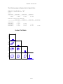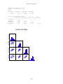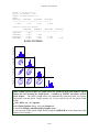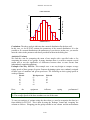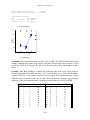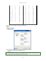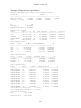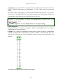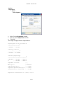
1
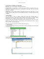
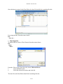
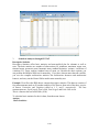
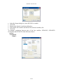
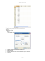
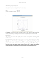
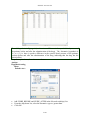
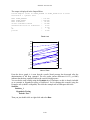
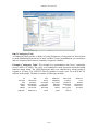
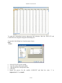
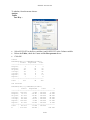
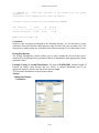
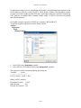
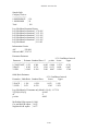
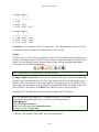
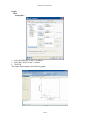
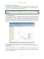
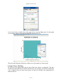
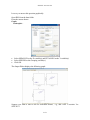
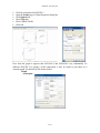
SYSTAT: AN OVERVIEW T. Krishnan Cranes Software International Limited, Mahatma Gandhi Road, Bangalore - 560 001 [email protected] 1. Introduction SYSTAT was designed for statistical analysis and graphical presentation of scientific and engineering data. In order to use this tutorial, knowledge of Windows 95/98/2000/Nt/XP would be helpful. SYSTAT provides a powerful statistical and graphical analysis system in a new graphical user interface environment using descriptive menus, toolbars and dialog boxes. It offers numerous statistical features from simple descriptive statistics to highly sophisticated statistical algorithms. Taking advantage of the enhanced user interface and environment, SYSTAT offers many major performance enhancements for speed and increased ease of use. Simply pointing and clicking the mouse can accomplish most tasks. SYSTAT provides extensive use of drag-ndrop and right click mouse functionality. SYSTAT’s intuitive Windows interface and flexible command language are designed to make your research more efficient. You can quickly locate advanced options through clear, comprehensive dialogs. SYSTAT also offers a huge data worksheet for powerful data handling. SYSTAT handles most of the popular data formats Excel, SPSS, SAS, BMDP, MINITAB, S-Plus, Statistica, Stata, JMP, and ASCII. All matrix operations and computations are menu driven. The Graphics module of SYSTAT 12 is an enhanced version of the existing graphics module of SYSTAT 11. This module has better user interactivity to work with all graphical outputs of the SYSTAT application. Users can easily create 2D and 3D graphs using the appropriate top tool bar icons, which provide tool tip descriptions of graphs. Graphs could be created from the Graph top tool bar menu or by using the Graph Gallery, which facilitate accomplishing complex graphs (e.g. global map with contour, 3D surface plots with contour projections, etc.) with point and click of a mouse. Simply double clicking the graph will bring up a dialog to facilitate editing most of graph attributes from one comprehensive 'dynamic dialogue'. Each graph attribute such as line thickness, scale, symbols choice, etc. can be changed with mouse clicks. Thus simple or complex changes to a graph or set of graphs can be made quickly and done exactly as the user requires. 2. Getting Started With SYSTAT 2.1 Opening SYSTAT for Windows To start SYSTAT for Windows NT4, 98, 2000, ME and XP: ¾ Choose: Start → All Programs→ SYSTAT 12→ SYSTAT 12 Alternatively, you can double-click on the SYSTAT icon , to get started with SYSTAT. SYSTAT: An Overview 2.2 User Interface The user interface of SYSTAT is organized into three spaces: I. Viewspace II. Workspace III. Commandspace The Screenshot of startpage of SYSTAT 12: I. Viewspace has the following tabs Output Editor: Graphs and statistical results appear in the Output Editor. You can edit, print and save the output displayed in the Output Editor. Data Editor: The Data Editor displays the data in a row-by-column format. Each row is a case and each column is a variable. You can enter, edit, view, and save data in the Data Editor. Graph Editor: You can edit and save graphs in the Graph Editor. Startpage: Startpage window appears in Viewspace as you open SYSTAT. It has five subwindows. i. Recent Files ii. Tips iii. Themes iv. Manuals v. Scratchpad You can resize the partition of the Startpage or you can close the startpage for the remainder of the session. If you want to view the Data Editor and the Graph editor simultaneously click Window menu or right-click in the toolbar area and select Tile or Tile vertically. I-134 SYSTAT: An Overview II. Workspace has the following tabs Output Organizer: The Output Organizer tab helps primarily to navigate through the results of your statistical analysis. You can quickly navigate to specific portions of output without having to use the Output Editor scrollbars. Examples: The Examples tab enables you to run the examples given in the user manual with just a click of mouse. The SYSTAT examples tree consists of folders corresponding to different volumes of user manual and nodes. You can also add your own example. Dynamic Explorer: The Dynamic Explorer can be used to rotate 3-D graphs, apply power transformations to values on one or more axes, and change the confidence intervals, ellipses, and kernels in scatter plots. By default, the Dynamic Explorer appears automatically when the Graph Editor tab is active. III. Commandspace has the following tabs Interactive: In the Interactive tab, you can enter commands at the command prompt (>) and issue them by pressing the Enter key. Untitled: The Untitled tab enables you to run the commands in the batch mode. You can open, edit, submit and save SYSTAT command file (.syc or .cmd) Log: In the Log tab, you can view the record of the commands issued during the SYSTAT session (through Dialog or in the Interactive mode). By default the tabs of Commandspace are arranged in the following order. Interactive Log Untitled You can cycle through the three tabs using the following keyboard shortcuts: CTRL+ALT+TAB. Shifts focus one tab to the right. CTRL+ALT+SHIFT+TAB. Shifts focus one tab to the left. I-135 SYSTAT: An Overview SYSTAT Data, Command and Output files Data files. You can save data files with (.SYZ) extension. Command files. A command file is a text file that contains SYSTAT commands. Saving your analyses in a command file allows you to repeat them at a later date. These files are saved with (.SYC) extension. Output files. SYSTAT displays statistical and graphical output in the output Editor. You can save the output in (.SYO), Rich Text format (.RTF) and HyperText Markup Language format (*.HTM). The Data Editor The Data Editor is used for entering, editing, and saving data. Entering data is a straightforward process. Editing data includes changing variable names or attributes, adding and deleting cases or variables, moving variables or cases, and correcting data errors. SYSTAT imports and exports data in all popular formats, including Excel, ASCII Text, Lotus, BMDP Data, SPSS, SAS, StatView, Stata, Statistica, JMP, Minitab and S-Plus as well as from any ODBC compliant application. Data can be entered or imported in SYSTAT in the following way: Entering data Consider the following data that has records about seven dinners from the frozen-food section of a grocery store. Brand$ Calories Fat Lean Cuisine 240 5 Weight Watchers 220 6 Healthy Choice 250 3 Stouffer 370 19 Gourmet 440 26 Tyson 330 14 Swanson 300 12 To enter these data into Data Editor, from the menus choose: File→ New→ Data This opens the Data Editor (or clears its contents if it is already open). I-136 SYSTAT: An Overview Before entering the values of variables you may want to set the properties of these variables using Variable Properties Dialog Box. To open Variable Properties Dialog Box form the menus choose: Data Variable Properties … Or right click (VAR) in the data editor and select Variable Properties. Or you can use CTRL+SHIFT+P. Type BRAND$ for the name. The dollar sign ($) at the end of the variable name indicates that the variable is a “string” or a “character” variable, as opposed to numeric variable. Note: Variable names can have up to 256 characters. Select String as the Variable type. Enter the number of characters in the “Characters” box. In the Comments box you can give any comment or description of the variable if you want. As here the variable BRAND$ is explained. Click OK to complete the variable definition for VAR_1. To type CALORIES as Variable name, again open the dialog box in the same way. Select Numeric as the Variable type. Enter the number of characters in the “Characters” box. [The decimal point is considered as a character.] Select the number of Decimal places to display. Click OK to complete the variable definition for VAR_2. Repeat this process for the FAT variable, selecting Numeric as the variable type or you can do the same in another way. Double-click (VAR) or click the Variable tab in data editor to get Variable Editor. With Variable Editor you can edit variables directly. I-137 SYSTAT: An Overview You can specify the properties of FAT variable in the same way in the third row. Now after setting the variable properties you can start entering data by clicking the Data tab in Data Editor. Click the top left data cell (under the name of the first variable) and enter the data. To move across rows, press Enter or Tab after each entry. To move down columns, press the down arrow key. Note: To navigate the behavior of the Enter key in the Data Editor. From the menus choose: Edit Options Data… Click either of the two radio buttons below Data Editor cursor. I-138 SYSTAT: An Overview Once the data are entered in the Data Editor, the data file should look something like this: For saving the data, from the menus choose: File Save As… Importing Data. To import IRIS.xls. (data of Excel format) from the menus choose: File Open Data... From the ‘Files of type’ drop-down list, choose Microsoft Excel. Select the IRIS.xls file. Select the desired Excel sheet and click OK. The data file in the Data Editor should look something like this: I-139 SYSTAT: An Overview 3. Statistical Analyses through SYSTAT Descriptive Statistics Descriptive Statistics offers basic statistics and stem-and-leaf plot for columns as well as rows. The basic statistics are: number of observations (N), minimum, maximum, mean, sum, trimmed mean, geometric mean, harmonic mean, standard deviation, variance, coefficient of variation (CV), range, median, standard error of mean, etc. Besides the above options, you can perform the Shapiro-Wilk test for normality. If you have chosen more than one variable, you can also compute multivariate statistics like multivariate skewness and multivariate kurtosis, and carry out the Henze-Zirkler multivariate normality test. Example: We will use the IRIS data to compute descriptive statistics. This data set consists of four measurements made on 50 random samples of Iris flowers from each of the three species of Setosa, Versicolor, and Virginica (coded as 1, 2, and 3, respectively). The four measurements are Sepal length, Sepal width, Petal length, and Petal width in cm. This is a famous data set from Fisher (1936). To calculate basic statistics for the iris data, from the menu choose: Analyze Basic Statistics… I-140 SYSTAT: An Overview Choose SEPALWID and add it to the Selected variable(s) list. Select N, Mean, SD, Minimum, Maximum. To check for normality, select the Shapiro-Wilk normality test option. Click OK. The following output is displayed in the Output Editor: N of cases Minimum Maximum Mean Standard Dev SW Statistic SW P-Value SEPALWID 150 2.000 4.400 3.057 0.436 0.985 0.101 Correlation The ‘Correlation’ feature computes correlations and measures of similarity and distance. Example: In the previous example, we computed basic statistics for SEPALWID. We will now compute the correlations between the four variables. Often, we may want to compute certain statistics separately for each group defined by certain variable(s) in the data set. In this case, we may want to examine if the correlations are of the same magnitude in the three species. SYSTAT facilitates such computations by its ‘By Groups’ feature. Let us use By Groups in the Data menu to request separate results for each level of SPECIES (grouping variables). From the menus choose: Data By Groups I-141 SYSTAT: An Overview In the By Groups dialog box, select SPECIES as variable. Click OK. Return to the Simple Correlations dialog box. Select all the four variables and add it to the Selected variable(s) list. Click OK. To compute correlations between pairs of the four variables: SEPALLEN, SEPALWID PETALLEN and PETALWID, from the menus choose: Analyze Correlations Simple... I-142 SYSTAT: An Overview The following output is displayed in the Output Editor: Results for SPECIES = 1.000 Number of Observations: 50 Means SEPALLEN SEPALWID PETALLEN PETALWID ----------------------------------------5.006 3.428 1.462 0.246 Pearson Correlation Matrix ¦ SEPALLEN SEPALWID PETALLEN PETALWID ---------+-----------------------------------------SEPALLEN ¦ 1.000 SEPALWID ¦ 0.743 1.000 PETALLEN ¦ 0.267 0.178 1.000 PETALWID ¦ 0.278 0.233 0.332 1.000 PETALWID PETALLEN SEPALWID SEPALLEN Scatter Plot Matrix SEPALLEN SEPALWID PETALLEN PETALWID I-143 SYSTAT: An Overview Results for SPECIES = 2.000 Number of Observations: 50 Means SEPALLEN SEPALWID PETALLEN PETALWID ----------------------------------------5.936 2.770 4.260 1.326 Pearson Correlation Matrix ¦ SEPALLEN SEPALWID PETALLEN PETALWID ---------+-----------------------------------------SEPALLEN ¦ 1.000 SEPALWID ¦ 0.526 1.000 PETALLEN ¦ 0.754 0.561 1.000 PETALWID ¦ 0.546 0.664 0.787 1.000 PETALWID PETALLEN SEPALWID SEPALLEN Scatter Plot Matrix SEPALLEN SEPALWID PETALLEN PETALWID I-144 SYSTAT: An Overview Number of observations: 50 Results for SPECIES = 3.000 Number of Observations: 50 Means SEPALLEN SEPALWID PETALLEN PETALWID ----------------------------------------6.588 2.974 5.552 2.026 Pearson Correlation Matrix ¦ SEPALLEN SEPALWID PETALLEN PETALWID ---------+-----------------------------------------SEPALLEN ¦ 1.000 SEPALWID ¦ 0.457 1.000 PETALLEN ¦ 0.864 0.401 1.000 PETALWID ¦ 0.281 0.538 0.322 1.000 PETALWID PETALLEN SEPALWID SEPALLEN Scatter Plot Matrix SEPALLEN SEPALWID PETALLEN PETALWID Quick Graphs. Quick Graphs are graphs which are produced along with numeric output without the user invoking the Graph menu. A number of SYSTAT procedures include Quick Graphs. The Quick Graphs above are automatically generated when you request correlations (with the Quick Graphs options on). If you want to turn off the Quick Graph facility: Under Edit menu, click Options. In the Global Options dialog, select the Output tab. Turn off the Display statistical Quick Graphs option. Or you can turn off the Quick Graph facility using the QGRAPH tab in the status bar at the bottom of user interface. I-145 SYSTAT: An Overview The above Quick Graphs in this example are in the scatterplot matrix (SPLOM). In each SPLOM there is one bivariate scatterplot corresponding to each entry in the correlation matrix that follows. A univariate histogram for each variable is displayed along the diagonal, and 75% normal distribution-based confidence ellipses are displayed within each plot. For species 3 (i.e., Virginica), the plot of SEPALLEN and PETALLEN has the narrowest ellipse, and thus, the strongest correlation, which is 0.864. Hypothesis Testing SYSTAT provides several parametric tests of hypotheses and confidence intervals for means, variances, proportions, and correlations. This section provides examples of the one-sample ttest and the paired t test. One-Sample t-test The one-sample t test is used to test if the mean of the population (from which the data set form a sample) is equal to a hypothesized value. Example: One-Sample test. Let us study the effect of cigarette smoking on the carbon monoxide diffusing capacity (DL) of the lung. Ronald Knudson, Walter Klatenborn, and Benjamin Burrows found that current smokers had DL readings significantly lower than those of exsmokers or nonsmokers. Let us find out if the data indicate that the mean DL (µ) reading for current smokers is significantly lower than 100 DL. The null hypothesis is Ho: µ = 100 against the alternative hypothesis H1: µ < 100 The carbon monoxide diffusing capacities for a random sample of n=20 are entered in the Data Editor. I-146 SYSTAT: An Overview To perform one-sample t-test, from the menus choose: Analyze Hypothesis testing Mean One-Sample t-test… Add DL_Reading to the Selected variable(s) list. Enter Mean 100. From the drop-down list, select the alternative type as ‘less than’. Click OK. I-147 SYSTAT: An Overview The following output is displayed: One-sample t-test of DL_READING with 20 Cases Ho: Mean = 100.00 vs Alternative = 'less than' Mean 95.00% Confidence Bound Standard Deviation t df p-value : : : : : : 89.855 95.617 14.904 -3.044 19 0.003 Conclusion: We observe that the one-sided p-value is 0.003, which is highly significant. Clearly, the mean DL (µ) reading for current smokers is significantly lower than 100 DL. Paired t-test The paired t-test assesses the equality of two means in experiments involving paired measurements. Example: Paired t-test. To illustrate the paired t-test we use the data from Hand et al. (1996). The data were collected on the systolic blood pressure of 15 patients (MacGregor et al., 1979). The interest is to see if there is any difference in the systolic blood pressure of the patients, before and after the administration of a drug called captopril. The BP data file gives the supine systolic and diastolic blood pressures (mm Hg) for 15 patients with moderate essential hypertension, immediately before and two hours after administering the drug. I-148 SYSTAT: An Overview The null hypothesis is Ho: µd = 0 (i.e. there is no difference in the systolic blood pressure of the patients, before and after the administration of the drug). The alternative hypothesis is H1: µd > 0 (i.e. there is positive difference in the systolic blood pressure of the patients, between before and after the administration of the drug, indicating that the drug has the desired effect.) To perform paired t-test, from the menu choose: Analyze Hypothesis testing Mean Paired t-test… Add SYSBP_BEFORE and SYSBP_AFTER in the Selected variable(s) list. From the drop-down list, select the alternative type as ‘greater than’. Click OK. I-149 SYSTAT: An Overview The output is displayed in the Output Editor. Paired Samples t-test on SYSBP_BEFORE vs SYSBP_AFTER with 15 Cases Alternative = 'greater than' Mean SYSBP_BEFORE Mean SYSBP_AFTER Mean Difference 95.00% Confidence Bound Standard Deviation of Difference t df p-value : 176.933 : 158.000 : 18.933 : 14.828 : 9.027 : 8.123 : 14 : 0.000 Paired t-test 220 210 200 Value 190 180 170 160 150 140 130 120 SYSBP_AFTER SYSBP_BEFORE Index of Case From the above graph, it is seen that the systolic blood pressure has decreased after the administration of the drug captopril. The test results (mean difference=18.933, p=0.000) indicate that the drug captopril reduces the systolic blood pressure. You can do the same testing using the Example tab of Workspace as this is already included as an example in Hypothesis testing of Statistics-I. So for running this example using the Examples tree (which is collapsible) first click the example tab in Workspace then click Statistics Statistics_1 Hypothesis Testing Paired t-Test… Then you just double-click or right-click and select Run. I-150 SYSTAT: An Overview R × C Contingency Table A contingency table provides a display of (joint) frequencies of categorical (or discrete) data to study relationships between two or more variables. Using Crosstabulation, you can analyze and save frequency tables that are formed by categorical variables. Example: Contingency Table. This example uses questionnaire data from a community survey (Afifi et al., 2004). The survey was conducted to study depression and help-seeking behavior among adults. The CESD depression index was constructed by asking people to respond to 20 items. The SURVEY2 data file includes a record (case) for each of the 256 subjects in the sample. The data set consists of following variables: ID INCOME SAD ENJOY MIND DRINK CHRONIC SEX RELIGION FEARFUL BOTHERED TALKLESS HEALTHY MARITAL$ AGE BLUE FAILURE NO_EAT UNFRNDLY DOCTOR SEX$ I-151 MARITAL DEPRESS AS_GOOD EFFORT DISLIKE MEDS AGE$ EDUCATN LONELY HOPEFUL BADSLEEP TOTAL BED_DAYS EDUC$ EMPLOY CRY HAPPY GETGOING CASECONT ILLNESS SYSTAT: An Overview To study the relationship between depression and education, label the EDUCATN and CASECONT into categories using the Label dialog box. To open the Label dialog box, from the menus choose: Data Label… Select EDUCATN as the variable. Type the value(s) that require labels. Type the label for each specified value. Click OK. Repeat the process for the variable CASECONT and label the value ‘1’ as depressed and ‘0’ as normal. I-152 SYSTAT: An Overview To tabulate, from the menus choose: Analyze Tables Two-Way… Select EDUCATN as the Row variable(s) and CASECONT as the Column variable. Below the Tables, check the Counts and the Row percents boxes. Click OK. Counts EDUCATN(rows) by CASECONT(columns) ¦ normal depressed Total --------+--------------------------Dropout ¦ 3 0 3 Dropout ¦ 33 14 47 HS grad ¦ 80 18 98 college ¦ 42 3 45 college ¦ 33 8 41 Degree+ ¦ 14 0 14 Degree+ ¦ 7 1 8 --------+--------------------------Total ¦ 212 44 256 Row Percents EDUCATN(rows) by CASECONT(columns) ¦ normal depressed ¦ Total N --------+---------------------+-----------------Dropout ¦ 100.000 0.000 ¦ 100.000 3.000 Dropout ¦ 70.213 29.787 ¦ 100.000 47.000 HS grad ¦ 81.633 18.367 ¦ 100.000 98.000 college ¦ 93.333 6.667 ¦ 100.000 45.000 college ¦ 80.488 19.512 ¦ 100.000 41.000 Degree+ ¦ 100.000 0.000 ¦ 100.000 14.000 Degree+ ¦ 87.500 12.500 ¦ 100.000 8.000 --------+---------------------+-----------------Total ¦ 82.813 17.188 ¦ 100.000 N ¦ 212.000 44.000 ¦ 256.000 I-153 SYSTAT: An Overview *** WARNING *** : More than One-fifth of the fitted Cells are sparse (Frequency < 5). Significance Tests computed on this table are Suspect. Chi-square tests of association for EDUCATN and CASECONT ¦ Test Statistic ¦ Value df p-value -------------------+------------------------Pearson Chi-square ¦ 12.645 6.000 0.049 Number of Valid Cases: 256 Conclusion: Subject to the reservation mentioned in the Warning message, we see that there is some association between Education and Depression state (p-value only just less than 0.05). The association is neither strong; nor is the direction of the association vis a vis Education is clear. Fitting Distributions The ‘Fitting Distributions’ feature enables you to assess whether the observed data can be modeled by a distribution from a parametric family of distributions with appropriately chosen parameter values. Example: Fitting of Normal Distribution. The data in FOREARM1 contains length of forearm (in inches) from Pearson and Lee (1903). A normal distribution may be an appropriate model to describe the data on the forearm length. To fit a normal distribution, from the menus choose: Analyze Fitting Distributions Continuous… I-154 SYSTAT: An Overview Add ARMLENGTH to the Selected variable(s) list. Select Distribution as Normal. Click OK. The output is displayed in the Output Editor: Variable Name : ARMLENGTH Distribution : Normal Estimated Parameter(s) Location or Mean(mu) : 18.802143 Scale or SD(sigma) : 1.116466 Estimation of Parameter(s): Maximum Likelihood Method Test Results Lower Limit Upper Limit Observed Expected ------------------------------------------------. 17.160000 11 9.893397 17.160000 17.690000 12 12.449753 17.690000 18.220000 16 19.802248 18.220000 18.750000 29 25.247070 18.750000 19.280000 22 25.802405 19.280000 19.810000 24 21.137956 19.810000 20.340000 11 13.880695 20.340000 . 15 11.786478 140 140.000000 Chi-square Test Statistic : 3.849814 Degrees of Freedom : 5 p-value : 0.571236 Kolmogorov-Smirnov Test Statistic : 0.047870 Lilliefors Probability : 0.554270 Shapiro-Wilk Test Statistic p-value : 0.991759 : 0.590263 I-155 SYSTAT: An Overview Fitted Distribution 30 0.2 Count 0.1 10 0 16 18 Proportion per Bar 20 0.0 22 20 ARMLENGTH Conclusion: The above analysis indicates that a normal distribution fits the data well. In this case, we let SYSTAT estimate the parameters of the normal distribution. It is also possible to fit a normal distribution with parameters of your choice; in that case, you need to enter the values in the parameter edit boxes provided for them in the dialog box. Analysis of Variance We used the t-test for comparing the mean of one sample with a specified value or for comparing the means of two groups. In many situations there is a need to compare several means and to test the significance of differences between three or more means from independently sampled populations. Example: One Way ANOVA. This example uses a one-way design to compare average typing speeds of three groups of typists. Fourteen beginning typists were randomly assigned to three types of machines and given speed tests. The following are their typing speeds in words per minute: Electric 52 47 51 49 53 Does the Word processor 67 73 70 75 64 equipment Plain old 52 43 47 44 influence typing performance? Ho: The average speeds of the three machines are the same. H1: The average speeds of the three machines are not all the same. To carry out analysis of variance using the above data, we need to reorganize the data in a form suitable for SYSTAT. This is done by using the `Reshape’ feature and `wrapping’ the columns as follows. Wrapping puts the group variable in one column and the measurement I-156 SYSTAT: An Overview variable in another column. Thus we need to wrap the data in two columns for which from the menus choose: Data Reshape Wrap/Unwrap….. The data file looks as follows: The variable MEASURE is the typing speed using three types of machines. The levels ‘1’, ‘2’ and ‘3’ correspond to machines ELECTRIC, WORD PROCESSOR and PLAIN OLD respectively in the TRIAL column. Of course, you might like to rename `Trial’ as `Equipment$’ and `Measure’ as `Speed’ using the Variable Properties dialog. Now let us do one-way analysis of variance using the wrapped data. To perform One-Way ANOVA, from the menus choose: Analyze Analysis of Variance Estimate Model… I-157 SYSTAT: An Overview Add MEASURE as the Dependent variable. Add TRIAL as the Factor. Click OK. The output is displayed in the Output Editor: Effects coding used for categorical variables in model. The categorical values encountered during processing are Variables ¦ Levels -----------------+------------------------------TRIAL (3 levels) ¦ 1.000000 2.000000 3.000000 1 case(s) are deleted due to missing data. Dependent Variable N Multiple R Squared Multiple R ¦ MEASURE ¦ 14 ¦ 0.952266 ¦ 0.906811 Analysis of Variance Source ¦ Type III SS df Mean Squares F-ratio p-value -------+------------------------------------------------------TRIAL ¦ 1469.357143 2 734.678571 53.519631 0.000002 Error ¦ 151.000000 11 13.727273 Least Squares Means Factor ¦ Level LS Mean Standard Error N -------+---------------------------------------------TRIAL ¦ 1 50.400000 1.656941 5.000000 TRIAL ¦ 2 69.800000 1.656941 5.000000 TRIAL ¦ 3 46.500000 1.852517 4.000000 I-158 SYSTAT: An Overview Durbin-Watson D Statistic ¦ 3.152318 First Order Autocorrelation ¦ -0.696026 Information Criteria AIC ¦ 81.025394 AIC (Corrected) ¦ 85.469838 Schwarz's BIC ¦ 83.581623 Least Squares Means 78.0 SPEED 69.8 61.6 53.4 45.2 pr oc es s w or d pl ai n el ec tri ol d c 37.0 EQUIPMNT$ Conclusion: We reject the hypothesis as the p-value is small. The Quick Graph illustrates this finding. Although the typists using electric and plain old typewriters have similar average speeds (50.4 and 46.5, respectively), the word processor group has a much higher average speed. Example: Two Way ANOVA. Consider the following data from a two-factor (Drug & Disease) experiment, from Afifi and Azen (1972), cited in Neter et al. (1996). The dependent variable, SYSINCR, is the change in systolic blood pressure after administering one of four different drugs to patients with one of three different diseases. Patients were assigned randomly to one of the possible drugs. The data are stored in the SYSTAT file AFIFI. S.no DRUG DISEASE SYSINCR S.no DRUG DISEASE SYSINCR 1 2 3 4 5 6 7 8 9 10 11 1 1 1 1 1 1 1 1 1 1 1 1 1 1 1 1 1 2 2 2 2 3 42 44 36 13 19 22 33 26 33 21 31 29 30 31 32 33 34 35 36 37 38 39 2 2 3 3 3 3 3 3 3 3 3 3 3 1 1 1 2 2 2 2 2 3 4 16 1 29 19 11 9 7 1 -6 21 I-159 SYSTAT: An Overview 12 13 14 15 16 17 18 19 20 21 22 23 24 25 26 27 28 1 1 1 1 2 2 2 2 2 2 2 2 2 2 2 2 2 3 3 3 3 1 1 1 1 1 2 2 2 2 3 3 3 3 -3 25 25 24 28 23 34 42 13 34 33 31 36 3 26 28 32 40 41 42 43 44 45 46 47 48 49 50 51 52 53 54 55 56 57 58 3 3 3 4 4 4 4 4 4 4 4 4 4 4 4 4 4 4 4 3 3 3 1 1 1 1 1 2 2 2 2 2 2 3 3 3 3 3 1 9 3 24 9 22 -2 15 27 12 12 -5 16 15 22 7 25 5 12 To perform Two-way ANOVA, from the menus choose: Analyze Analysis of Variance Estimate Model… Select SYSINCR as the Dependent variable. Add DRUG and DISEASE in the Factor list box. Click OK. Note: While performing ANOVA, all interaction terms are included in the analysis. If you want to specify your own model then use the ‘GLM’ feature. I-160 SYSTAT: An Overview The output is displayed in the Output Editor: Effects coding used for categorical variables in model. The categorical values encountered during processing are Variables ¦ Levels -------------------+-----------------------------------------DRUG (4 levels) ¦ 1.000000 2.000000 3.000000 4.000000 DISEASE (3 levels) ¦ 1.000000 2.000000 3.000000 Dependent Variable N Multiple R Squared Multiple R ¦ SYSINCR ¦ 58 ¦ 0.675296 ¦ 0.456024 Analysis of Variance Source ¦ Type III SS df Mean Squares F-ratio p-value -------------+-----------------------------------------------------DRUG ¦ 2997.471860 3 999.157287 9.046033 0.000081 DISEASE ¦ 415.873046 2 207.936523 1.882587 0.163736 DRUG*DISEASE ¦ 707.266259 6 117.877710 1.067225 0.395846 Error ¦ 5080.816667 46 110.452536 Least Squares Means Factor ¦ Level LS Mean Standard Error N -------+----------------------------------------------DRUG ¦ 1 25.994444 2.751008 15.000000 DRUG ¦ 2 26.555556 2.751008 15.000000 DRUG ¦ 3 9.744444 3.100558 12.000000 DRUG ¦ 4 13.544444 2.637123 16.000000 Least Squares Means Factor ¦ Level LS Mean Standard Error N --------+----------------------------------------------DISEASE ¦ 1 21.816667 2.492580 19.000000 DISEASE ¦ 2 19.745833 2.445986 19.000000 DISEASE ¦ 3 15.316667 2.374380 20.000000 Least Squares Means Factor ¦ Level LS Mean Standard Error N -------------+---------------------------------------------DRUG*DISEASE ¦ 1*1 29.333333 4.290543 6.000000 DRUG*DISEASE ¦ 1*2 28.250000 5.254820 4.000000 DRUG*DISEASE ¦ 1*3 20.400000 4.700054 5.000000 DRUG*DISEASE ¦ 2*1 28.000000 4.700054 5.000000 DRUG*DISEASE ¦ 2*2 33.500000 5.254820 4.000000 DRUG*DISEASE ¦ 2*3 18.166667 4.290543 6.000000 DRUG*DISEASE ¦ 3*1 16.333333 6.067744 3.000000 DRUG*DISEASE ¦ 3*2 4.400000 4.700054 5.000000 DRUG*DISEASE ¦ 3*3 8.500000 5.254820 4.000000 DRUG*DISEASE ¦ 4*1 13.600000 4.700054 5.000000 DRUG*DISEASE ¦ 4*2 12.833333 4.290543 6.000000 DRUG*DISEASE ¦ 4*3 14.200000 4.700054 5.000000 Durbin-Watson D Statistic ¦ 2.413731 First Order Autocorrelation ¦ -0.223131 Information Criteria AIC ¦ 450.018358 AIC (Corrected) ¦ 458.291085 Schwarz's BIC ¦ 476.804117 I-161 SYSTAT: An Overview Conclusion: In two-way ANOVA, begin the analysis by looking at the interaction effect. The DRUG * DISEASE interaction is not significant (p = 0.396), so shift your focus to the main effects. The DRUG effect is significant (p < 0.0005), but the DISEASE effect is not (p = 0.164). Thus, at least one of the drugs differs from the others with respect to blood pressure change, but blood pressure change does not vary significantly across diseases. Note: Along with ANOVA table, SYSTAT also displays the Estimates of the model parameters. To get the estimates, you need to select LONG as the PLENGTH option. To do so, from the menus, choose Edit ÆOptions. Select the Output tab. From the Output results, select Length as Long. Linear Regression Regression analysis is used to investigate a predictive relationship between a response variable and one or more predictors. Example: Let us study the relationship between noise exposure (predictor or independent variable) and hypertension (dependent or response variable). The following data were collected on Y (blood pressure rise in millimeters of mercury) and X (sound pressure level in decibels). Y X 1 60 0 63 1 65 2 70 5 70 1 70 4 80 6 90 2 80 3 80 5 85 4 89 6 90 8 90 4 90 5 90 7 94 9 100 7 100 6 100 To perform Linear Regression, from the menus choose: I-162 SYSTAT: An Overview Analyze Regression Linear Least Squares… Select Y as the Dependent variable. Select X as the Independent variable. Click OK. The output is displayed in the Output Editor: Eigenvalues of Unit Scaled X'X 1 2 ------------------1.989028 0.010972 Condition Indices 1 2 -------------------1.000000 13.463989 Variance Proportions ¦ 1 2 ---------+-------------------CONSTANT ¦ 0.005486 0.994514 X ¦ 0.005486 0.994514 Dependent Variable N Multiple R Squared Multiple R Adjusted Squared Multiple R Standard Error of Estimate ¦ ¦ ¦ ¦ ¦ ¦ Y 20 0.865019 0.748257 0.734271 1.317963 Regression Coefficients B = (X'X)^{-1}X'Y I-163 SYSTAT: An Overview Std. Effect ¦ Coefficient Standard Error Coefficient Tolerance t p-value --------+----------------------------------------------------------------------CONSTANT¦ -10.131538 1.994900 0.000000 . -5.078720 0.000078 X ¦ 0.174294 0.023829 0.865019 1.000000 7.314472 0.000001 Confidence Interval for Regression Coefficients ¦ 95.0% Confidence Interval Effect ¦ Coefficient Lower Upper VIF ---------+----------------------------------------------------CONSTANT ¦ -10.131538 -14.322667 -5.940408 . X ¦ 0.174294 0.124232 0.224356 1.000000 Analysis of Variance Source ¦ SS df Mean Squares F-ratio p-value -----------+----------------------------------------------------Regression ¦ 92.933525 1 92.933525 53.501505 0.000001 Residual ¦ 31.266475 18 1.737026 *** WARNING *** : Case 5 is an Outlier (Studentized Residual : 2.740993) Durbin-Watson D Statistic ¦ 2.289856 First Order Autocorrelation ¦ -0.179127 Information Criteria AIC ¦ 71.693825 AIC (Corrected) ¦ 73.193825 Schwarz's BIC ¦ 74.681021 Conclusion. The estimates of the regression coefficients are -10.132 and 0.174, so the regression equation is: Y= -10.132 +0.174X F-ratio in the analysis of variance table is used to test the hypothesis that the slope is 0 (or, for multiple regressions, that all slopes are 0). The F is large when the independent variable(s) helps to explain the variation in the dependent variable. Here, there is a significant linear relation between Y and X. Thus, we reject the hypothesis that the slope of the regression line is zero (F-ratio = 53.502, p value (P) < 0.0005). SYSTAT also outputs statistics and warnings for outlier detection and for testing the assumptions in linear regression methodology. Logistic Regression Logistic regression describes the relationship between a dichotomous response variable and a set of explanatory (predictor or independent) variables. The explanatory variables may be continuous or (dummy variables) discrete. Example: Binary Logistic Regression. To illustrate the use of binary logistic regression, we consider this example from Hosmer and Lemeshow (2000). The purpose is to analyse low infant birth weight (LOW) as a function of several risk factors. I-164 SYSTAT: An Overview For the present analysis we are considering only mother’s weight during last menstrual period (LWT) and race (RACE=1:white, RACE=2: black, RACE=3:other). The dependent variable is coded 1 for birth weights less than 2500 gms. and coded 0 otherwise. Instead of considering LWT itself we are taking LWD, a dummy variable coded 1 if LWT is less than 110 pounds and coded 0 otherwise. Our model is simple regression of LOW on a constant, LWD and RACE. To perform Logistic regression, from the menus choose; Analyze Regression Logit Estimate Model… Select FALL as the Dependent variable. Select DIFFICULTY and SEASON as the Independent variables. The categorical values encountered during processing are Variables ¦ Levels ---------------+-------------LOW (2 levels) ¦ 0.000 1.000 Binary LOGIT Analysis Dependent Variable : LOW Input Records : 189 Records for Analysis : 189 I-165 SYSTAT: An Overview Sample Split Category Choices ----------------+---0 REFERENCE ¦ 130 1 RESPONSE ¦ 59 Total ¦ 189 Log-Likelihood Iteration History Log-Likelihood at Iteration1 ¦ -131.005 Log-Likelihood at Iteration2 ¦ -112.159 Log-Likelihood at Iteration3 ¦ -111.995 Log-Likelihood at Iteration4 ¦ -111.995 Log-Likelihood at Iteration5 ¦ -111.995 Log-Likelihood ¦ -111.995 Information Criteria AIC ¦ 229.989 Schwarz's BIC ¦ 239.715 Parameter Estimates 95 % Confidence Interval Parameter ¦ Estimate Standard Error Z p-value Lower Upper ------------+-----------------------------------------------------------------1 CONSTANT¦ -1.535 0.380 -4.043 0.000 -2.278 -0.791 2 RACE ¦ 0.263 0.176 1.501 0.133 -0.081 0.607 3 LWD ¦ 0.982 0.366 2.681 0.007 0.264 1.700 Odds Ratio Estimates ¦ 95 % Confidence Interval Parameter ¦ Odds Ratio Standard Error Lower Upper ----------+---------------------------------------------------------2 RACE ¦ 1.301 0.228 0.923 1.836 3 LWD ¦ 2.671 0.978 1.302 5.476 Log-Likelihood of Constants only Model = LL(0): -117.336 2*[LL(N)-LL(0)] : 10.683 df :2 p-value : 0.005 McFadden's Rho-squared ¦ 0.046 Cox and Snell R-square ¦ 0.055 Naglekerke's R-square ¦ 0.077 I-166 SYSTAT: An Overview Covariance Matrix ¦ 1 2 3 --+-----------------------1 ¦ 0.144 2 ¦ -0.058 0.031 3 ¦ -0.023 -0.007 0.134 Correlation Matrix ¦ 1 2 3 --+------------------------1 ¦ 1.000 -0.867 -0.165 2 ¦ -0.867 1.000 -0.108 3 ¦ -0.165 -0.108 1.000 Conclusion. We see that only RACE is significant. The likelihood-ratio statistic of 10.683 is chi-squared with two degrees of freedom and a p-value of 0.005. Graphs SYSTAT offers a wide variety of graphical analysis tools that enable better visualization of the data. The editing options in SYSTAT allow you to fine-tune and change the display of the graph. To create Summary charts, Density displays, Plots click on the graph toolbar menu or select the icon from the Graph toolbox Note. Graph menus are available when a data file is in use. Example: Simple Scatter Plot. Let us create a simple scatter plot. Consider the following data file. In various international cities, how long must people work to earn enough to buy a Big Mac? How does this time relate to the length of a typical work week? We plot BIG_MAC, the working time (in minutes) to buy a Big Mac against WORKWEEK, the length of the work week (in hours). The data are in the RCITY file that has 46 cases, one for each city. Open the RCITY.SYZ data file from DATA folder of main SYSTAT directory. Note. By default, the file location is “C:\Program Files\SYSTAT 12\Data” You can also change the default path. To do so, from the menus choose: Edit ÆOptions. Select the File Locations tab. Select the radio button, Set custom directories. Change the path for Open data. To plot Big_Mac against WORKWEEK, from the menus choose: I-167 SYSTAT: An Overview Graph Plots Scatterplot… Select WORWEEEK as the X-variable(s). Select BIG_MACK as the Y variable. Click OK. The Output Editor displays the following graph: I-168 SYSTAT: An Overview Customization of an existing graph Once you have created a graph, you can use the Graph Editor tab to change many of its features without recreating the graph. Using the Graph menu, you can change the properties such as color, axes, labels, symbols, titles and graph size. Note: To view the graph in the Graph Editor, either double-click on it or click the Graph Editor tab or double click the corresponding node in the tree formed in the Output Organizer. ¾ To Edit Graph Axes For editing graph axes as well as editing the graph as a whole you can use Graph Properties Dialog Box in the Graph Editor. To open the Graph Properties Dialog box, double-click on the Graph Editor. You can also right-click on the Graph Editor, open a menu with item ‘Properties’ at the top and click ‘Properties’ to open Graph Properties dialog box. Through the Graph Properties dialog box you can modify features of a graph, frame, axis, legend and element. For editing graph axes select the Axes page of the Graph Properties dialog box. The Axes dialog enables you to alter the axes of your graphs. It has four tabs Display, Font, Option and Line. Suppose now you find that X-axis label ‘WORKWEEK’ is difficult to comprehend and you want to make it more explanatory by changing the label, using the Graph Properties dialog box. Select the Display tab. I-169 SYSTAT: An Overview Display tab To enter the new label for the x-axes select `bottom’ from the drop down list. Change the WORKWEEK in the X-axis label to Average working hours per week. Click Ok. Now the X-axis label will be changed into AVERAGE WORKING HOURS PER WEEK.If you want to change the labels of other axes also proceed in a similar way. Note: Using the same dialog box you can specify suitable ranges for different axes using the Minimum and Maximum boxes. For a better specification, you can specify the number of ‘Tick Mark Intervals’ you want using the labeled(Tick) and Unlabeled(pip) boxes. You can also give a title for the graph using the same dialog box. Go to the Graph page. Click Options tab. Check the Title box. Enter a new title for your graph, say, WORKWEEK vs. BIG_MACK. For a better presentation, you may want to color the graph. Check Color box and select a suitable color. I-170 SYSTAT: An Overview You can also select a suitable font for the graph title by using the Font option. See this graph as an example, which is Algerian bold underline uppercase size 10. Thus the Graph Properties Dialog box enables you to edit graphs in various modes. Example: Fisher’s IRIS Data We again use the famous IRIS data set from Fisher and explore it graphically. We have already found that SEPALLEN and PETALLEN have the strongest correlation for SPECIES 3 (i.e., Virginica). Now you may want to know: are these two variables vary substantially for different species? I-171 SYSTAT: An Overview Let us try to answer this question graphically. Open IRIS from the data folder. From the menus choose: Graph Scatterplot… Select SEPALLEN as the X-variable(s) and PETALLEN as the Y-variable(s). Select SPECIES as the Grouping variable(s). Click OK. The Output Editor displays the following graph: Suppose you want to enter a title for individual frames, e.g., add a title ‘Versicolor’ for SPECIES 2. I-172 SYSTAT: An Overview Click the scatterplot for SPECIES 2. Open the Frame page of Graph Properties dialog box. Click Options tab. Check Title box. Write VERSICOLOR. Click OK. Now from the graph it appears that PETALLEN and SEPALLEN vary substantially for different SPECIES. For getting a better impression, it may be useful to plot them on a common graph. For thism from the menus choose: Graph Scatterplot… I-173 SYSTAT: An Overview Select SEPALLEN as the X-variable(s) and PETALLEN as the Y-variable(s). Select SPECIES as the Grouping variable(s). Check the Overlay mode. Click OK. The Output Editor displays the following graph: Now from the graph it is clear that PETALLEN and SEPALLEN vary significantly from one species to another. Now if you want to label the SPECIES go to the Legend page of the Variable Properties dialog box. Note that in the Overlay mode, Legend tab is activated. Select ‘1’ from the drop-down list of Label. Write ‘Setosa’ in the Change to box. Select ‘2’ from the drop- down list and write ‘Versicolor’. Select ‘3’ from the drop-down list and write ‘Virginica’. I-174 SYSTAT: An Overview In the Graph Editor, the legend labels are changed accordingly. Note that if you do not want to display legends, just uncheck the Display legend checkbox. You can also choose the symbols for different SPECIES. ¾ To Edit Appearance of the Graph: We have already customized some aspects of the appearance of a graph. Here are some more aspects: The Variable Properties dialog box will enable you to customize some more aspects. Using the Graph Properties dialog box you can change font, color, symbol, style, fill pattern etc. SYSTAT allows you to set color for fonts, symbol fill, symbol boundary, tick marks, axes lines, and elements, by choosing a color from the color palette that pops up by pressing of the corresponding color picker button. In the Color Palette, apart from the 48 predefined I-175 SYSTAT: An Overview colors, you can access more than 16 million colors using Define Custom Colors. Simply specify the RGB (Red-Green-Blue) or Hue-Sat-Lum (Hue-SaturationLuminosity) values, use the slider on the right to adjust the shading and press Add to Custom color. Suppose you want to highlight the points for SETOSA SPECIES. Select Setosa from the drop-down list of labels. Go to the Elements page. Click the Symbols tab. Select suitable options. Note: The above menus are also available in the main Scatterplot dialog box. To change the color of the elements in the graph, select the option Select color. Select a color from the Color drop-down list for each of the y variables. Select the fill pattern from fill tab. Select the symbols from symbol tab. I-176 SYSTAT: An Overview Fill To change the fill pattern for the elements in a graph, select the option Select fill. Select a fill pattern from the Fill Pattern drop-down list for each of the y variables. Symbol and Label You can change the symbol type by using any of SYSTAT’s 23 built-in symbols. Getting Help SYSTAT uses the standard HTML Help system to provide information you need to use SYSTAT and to understand the results. This section contains a brief description of the Help system and the kinds of help provided with SYSTAT. The best way to find out more about the Help system is to use it. You can ask for help in any of these ways: I-177 SYSTAT: An Overview Click the button in a SYSTAT dialog box. This takes you directly to a topic describing the use of the dialog box. This is the fastest way to learn how to use a dialog box. Right-click on any dialog box item, and select 'What's this?' to get help on that particular item. Select Contents or Search from the Help menu. For help on commands, from the command prompt (on the Interactive tab of the Commandspace) type: HELP [command name] References Afifi, A. A., May, S., and Clark, V. (1984). Computer-aided multivariate analysis, 4th ed. New York: Chapman & Hall. Fisher, R. A. (1936). The use of multiple measurments in taxonomic problems. Annals of Eugenics, 7, 179-188. Hand, D. J., Daly, F., Lunn A. D., McConway, K. J. and Ostrowski, E. (Editors) (1996). A handbook of data sets. London: Chapman & Hall Hosmer, D. W. and Lemeshow, S. (2000). Applied logistic regression 2nd ed. New York: John Wiley & Sons. Neter, J., Kutner, M.H., Nachtsheim, C.J., and Wasserman, W. (1996). Applied linear regression models. Homewood, IL: Irwin. Pearson, K. and Lee, A. (1903). On the laws of inheritance in man. I. Inheritance of physical characters. Biometrika, 2, 357—462. I-178