Download The General Feedback Theorem: A Final Solution for

V2
+
R3
200
i(V2)
i(V4)
rm3
50
rm4
10
+
V3
i(V1)
R8
10 MB
rm1
50
Rs
100
i(V3)
rm2
200
+
V4
Cc
20p
uo
ui
V1
+
+
+
R2
900
−
RL
1k
>
Error Voltage
R1
100
Error Current
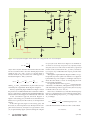
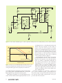
Figure 7. A simple feedback amplifier model with the error voltage and the error current identified.
H = H∞
1
Tn
1 + T1
1+
,
(15)
and, in this form, the dissection theorem becomes the GFT.
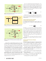
For the second-level TFs to have the desired physical interpretations TF1 = H∞ , TF2 = T, TF3 = Tn , the test signal uz
must be inside the loop and at the error summing point, as
illustrated in Figure 5. Then, (8) becomes
H∞ ≡
uy uy uo T
≡
T
≡
.
n
ui uy=0
ux ui =0
ux uo =0
(16)
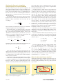
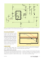
With H∞ , T, and Tn calculated from (16), the result (15) is represented by the “augmented” block diagram of Figure 6.
Because, superficially, Figure 6 differs from Figure 1 only in
the presence of an additional block that contains the nonidealities, it is important to emphasize the fundamental difference
between the conventional approach and that based on the GFT.
In the conventional approach, the block diagram of
Figure 1 is the starting point, in which reverse transmission in
both boxes is ignored, and the result (2) is developed from
Figure 1.
In the GFT approach, Figure 5 is the starting point, and
the result (15) is developed from (16) directly from the complete circuit without any assumptions or approximations. Since
(15) is represented by Figure 6, the block diagram of Figure
56
6 is part of the result. The boxes in Figure 6 are unidirectional and do not necessarily correspond to any separately identifiable parts of the circuit. The values of these boxes, expressed
in terms of the second level TFs H∞ , T, and Tn , automatically incorporate any nonidealities that may be present in the
actual circuit.
Although the augmented block diagram exhibits a “loop,”
it represents any linear system even if there is not a physically discernible loop. An example is a Darlington follower, for
which the GFT affords a means of investigating the wellknown potential instability.
It is apparent that the null loop gain Tn contains the firstorder effects of nonidealities, although there may also be second-order effects upon the loop gain T. Thus, the T in (2) may
not be the same as the correct T in (15).
Since it was convenient in (5) to introduce the discrepancy
factor D as a unique function of T, it is likewise useful to introduce the null discrepancy factor Dn as a unique function of
Tn , according to
Dn ≡
1 + Tn
1
≡1+
≡ null discrepancy factor
Tn
Tn
(17)
so that the final result for the first level TF T can be written
H = H∞ DDn .
(18)
April 2006