1
Distribution Pipe 1-2
User Manual
16.06.2014
How to use the Distribution Pipe tool
1) Create a simultaneous curve adapted to your context or choose an existing one
2) Use the table for quick calculation of your distributions pipes
3) Make accurate design with the calculation sheet
1. Define the specific simultaneous curve for your context
If the water consumption pattern in your
context differs from the western standards
(at least one tap per person with a
consumption up to 200 liters per day per
person) it might be good to define a
specific simultaneous curve for your
context.
Before starting to use this tool, you should
have defined the daily demand pattern
according to the chapter 1: Water
demand.
1) PT (peak time in hours): Define the peak or high demand time, this is the time during which
the demand is expected to be important, it can be taken as the time where the demand
ratio is higher than 100%, generally should be between 8 and 14 hours.
2) PWd (Peak water demand in liter): Define the average water demand at a tap during the
defined peak time; this represent usually between 70 to 95% of the total demand of the tap
for all the day.
3) Q (Flow in liter per second): Define the average expected flow
PT
15
hours
at your tap, this can range from 0.1 liter per second up to 0.3
PWd
2 365 l
liter per second, a good value is 0.2 l/s.
Q
0.20
l/s
If you have accurate figures for the pattern, another option is to work just with the peak hour.
IN this case the Peak time is one hour, the PWd is the daily consumption divided by 24 times
the peak factor.
The Excel Sheet will calculate the time during which your tap need to be open to deliver the
required quantity with the given flow (WT=PWD/Q in minutes), obviously this time should be
shorter than the peak time. If it is the same or close to it, it means that the taps are almost
always open, in this case there is no need to work with the simultaneous factor, it can just be
estimated that all taps are open at the same time and the design done with a continuous flow.
Then it will calculate the percentage of the time during which the
tap will deliver water during the peak time, or in other word the
probability that the tap is open (Prob = working time per peak
time =WT/PT).
WT
Prob
197 min
22% %
4) The last figure to enter is the maximum time during which it
T out
20.0 sec
is acceptable to have more taps open than the design value,
T out %
0.04% %
in other words the time during which the actual pressure and
flow will be lower than the design.
This value will give the probability for the cumulative binomial distribution, it should be of
few seconds (1 to 30) and give a ratio with the time span between 0.2% and 0.01%.
Tutorial on Distirbution Pipe.docx
1/5
LWI
Distribution Pipe 1-2
User Manual
16.06.2014
The following information is displayed:
Flow Total
N
Binomial
Fsim
N: is the number of taps connected to a pipe
(l/s)
flow
1
1 0.00% 100.0% 100.0% 0.200 0.20
Binomial 1st column: is the maximum number of tap open
2
2 0.00% 100.0% 100.0% 0.200 0.40
3
3 0.00% 100.0% 100.0% 0.200 0.60
at the same time respecting the condition T out. It is
4
4 0.00% 100.0% 100.0% 0.200 0.80
known as the inverse or negative binomial law.
5
5 0.00% 100.0% 94.0%
0.188 0.94
6
5 0.01% 83.3% 87.5%
0.175 1.05
Binomial 2nd column: is the probability of failure with the
7
6 0.00% 85.7% 82.5%
0.165 1.16
given number of tap, for instance with a total of 6 taps,
8
6 0.02% 75.0% 78.5%
0.157 1.26
9
7 0.00% 77.8% 75.2%
0.150 1.35
5 or less taps will be open 99.99% of the time, 6 taps
10
7 0.02% 70.0% 72.4%
0.145 1.45
will only be open 0.01% of the time.
Binomial 3rd column: is the ratio between the tap open and tap closed for the binomial
distribution, representing the proportion of taps to be assumed open. It is represented on
the chart by the red line.
Fsim: is the regression of the binomial 3rd column according to the
a
0.206
𝑏
following function: 𝐹𝑠𝑖𝑚 = a +
with the constant calculated by the
b
√𝑁+𝑐
1.63
macro when the button “Calc abc” is clicked. It is represented on the
c
-0.03
chart by the purple line.
Flow (l/s): is the average probable flow per tap using the regression curve
Total flow: (l/s) is the total probable flow to use to design a pipe connected to N taps.
If you see a warning “Too steep”, this mean that your regression curve is too sudden and that
the total flow will indeed decrease, which is physically impossible. This is usually due to a Tout
too small or too big for taps with small daily demand. If you don’t manage to correct it by
changing the Tout, the best is to adjust manually the constants a, b, and c.
On the chart you will see in red the binomial
distribution according to the given
specification. You can play a bit with the
different figures to see their influence on the
Binomial distribution.
The purple line represent the regression
with the constant a, b, and c.
The other curves represent predefined
distribution that should guide you to define
your curve.
Std tap: is the curve respecting the French standard (DTU
60-1 defining plumbing calculation). In most of developing
countries the quantity of water distributed per tap is much
higher, thus it can be assumed that this curve shows the
minimum requirement.
Heavy usage: this curve represent also a rather small
demand per tap but with a situation where simultaneous flow
can be expected to be important such as in a hotel or school.
Max: represent
N
1
2
3
4
5
6
7
8
9
10
Std tap
100%
80%
57%
46%
40%
36%
33%
30%
28%
27%
Heavy
usage
100%
100%
100%
100%
92%
82%
75%
70%
66%
62%
Max
100%
100%
100%
100%
100%
98%
96%
94%
92%
90%
Once you are happy with your distribution, click on the button “Calc abc” this will calculate the
constant values of a regression curve 𝐹𝑠𝑖𝑚 = a + 𝑏/√(𝑁 + 𝑐) best fitting the given distribution.
You can still play a bit with the values a, b and c and round them to have a clean function.
Tutorial on Distirbution Pipe.docx
2/5
LWI
Distribution Pipe 1-2
User Manual
16.06.2014
The constant a represent the horizontal asymptote towards which the function will converge,
thus it should be smaller than the average flow: 𝑎 ≈ 𝐷𝑊𝑑 ∙ 𝑃𝐹/(24 ∙ 3600 ∙ 𝑄). The constant c
define the beginning of the curve and is closely link to the binomial criteria, ranging from 5 to 5. The constant b define the curvature and range usually from 0.5 to 3.
To compare the simultaneous factor with the peak factor, you have
the possibility to enter it PF, with the Daily Water (not only the peak),
thus the average flow per tap (AFT) can be calculated and
compared to the flow per tap of the regression of the binomial
distribution.
PF
DWd
AFT
MTDP
200%
2 500
0.058
400
For a certain number of taps, the AFT might be bigger than the flow obtain with the
simultaneous factor. Then for pipes delivering water to more taps, the flow obtain with the peak
factor should be used. This approximate number of taps is given in as MTDP: minimum number
of taps to use the demand pattern. This value closely linked with a constant, if you want to use
only the simultaneous factor, use a as the asymptote, if you want to use quickly the demand
pattern, take it a small as reasonably possible (it means where your regression curve is not
too far from the binomial distribution).
2. Practical use of results with the Table
The table on the next Tab can be used to select quickly diameters of plastic pipes for simple
situations.
First the average flow per tap in liter per second should be given.
Then the SDR (Standard Dimensional Ratio is the outside diameter
divided by the thickness) of the pipe selected. If the calculation is done
for another fluid than water, the viscosity (Nu) can be changed.
Q
0.20
NU
1E-06
SDR
13.5
The minimum and maximum accepted water speed in the pipe can be
modified. Head losses will be shown only for pipe diameter respecting these
criteria.
The two columns below will give the maximum and minimum diameter
respecting the speed limits.
a
b
c
0.21
1.60
-0.50
N
1
2
3
4
l/s
Speed
0.5
1.5
Diameter
Min Max
13
23
18
32
23
39
26
45
The constant a, b, and c of the first tab will be used to calculate
the simultaneous factor. If you want to use other values, you
can just change them but be aware that the link will then be
lost.
N
Fsim
Flow
1
2
3
1.00
1.00
1.00
0.20
0.40
0.60
Tutorial on Distirbution Pipe.docx
In the column below, the Fsim is calculated for certain number
of taps and the probable flow calculated. This flow will be used
to calculate the head losses in the pipes.
3/5
LWI
Distribution Pipe 1-2
User Manual
The table will give the head losses in meter per
100m of pipe for the admissible diameter,
according to the number of downstream taps.
OD
ID
N
1
2
3
4
5
6
7
8
9
10
For instance a pipe connected to 2 taps can be
selected of 3 different diameters, the smallest
one of OD 20mm will have losses of 21.8 m (or
2.1 bar) per 100 m of pipes, the medium one of
OD 25mm will have losses of 7.46 m/100m,
and the largest one of 32mm will have losses
of 2.3 m/100m.
Length
P1
P2
P3
P4
P5
500
400
500
400
150
N° of
taps
10
5
2
1
1
Selected
OD
50
40
25
25
20
Losses
coeff
2.69
3.74
7.46
2.23
6.48
16
13.6
Head losses in meter for 100m length
20
25
32
40
50
17.0
21.3
27.3
34.1
42.6
18.69
-
6.48
21.82
-
5 taps
The attached scheme illustrates a short
distribution system deserving 10 taps.
Using the previous simultaneous factor,
flow and SDR, we can quickly find the
head losses for each as shown in the next
table. Assuming an available head of 80m.
Pipe
16.06.2014
P1
2.30
4.67
7.76
10.80
13.00
-
1.62
2.69
3.74
4.50
5.28
6.09
6.92
7.78
0.93
1.30
1.56
1.83
2.11
2.39
2.69
0.61
0.70
0.79
0.89
3 taps
P2
400 m
Losses/
section
13.5
15.0
37.3
8.9
9.7
2.23
7.46
15.23
-
63
53.7
P3
P5
P4
500 m
The total losses for the first tap is of:
ΔH = 13.5+15+37.3+8.9= 74.7m,
leaving a marge of ~5m of pressure.
For the second tap:
ΔH = 13.5+15+37.3+9.7= 75.5m, with
a marge of ~4.5m of pressure.
The calculation should be first done for the longest section, which will define the smallest
admissible pipe diameter that can be used, then the shortest section can be calculated.
If there is too much head losses with the biggest admissible pipes (smallest losses), other
solutions should be studied such as changing the layout, installing a equalization tank or
increasing the delivery pressure.
Tutorial on Distirbution Pipe.docx
4/5
LWI
Distribution Pipe 1-2
User Manual
16.06.2014
3. Make accurate design with the calculation sheet
In the next tab, you access to the real design tool, it works the same way as Gravity pipe, kindly
refer to its tutorial to know how to use it more in details.
Use the “Edit Nodes” command to add, delete or change types of nodes.
Fill-in all the yellow cells with the base data: Description, Taps, Elevation, Length, Roughness
and Sing. losses. Then adjust the diameters so that the energy is dropping regularly.
Tutorial on Distirbution Pipe.docx
5/5
LWI