
1
USER
MANUAL
Version 2.0 for Microsoft® Windows
MasterPlex QT
TM
Multiplex Data Analysis Software
MiraiBio
A
H I T A C H I
For Research Use Only
S O F T W A R E
C O M P A N Y
1201 Harbor Bay Parkway
Suite 150
Alameda, CA 94502
TELEPHONE
1.800.624.6176
1.510.337.2000
FACSIMILE
1.510.337.2099
Part no. P-33020-10200
TRADEMARKS
MicroSoft® is a registered trademark of Microsoft Corporation.
COPYRIGHT
© 2001-2003 MiraiBio, Inc. All Rights Reserved.
LICENSE AGREEMENT
LICENSE AGREEMENT
BEFORE OPENING THIS PACKAGE, YOU SHOULD
CAREFULLY READ THE FOLLOWING TERMS AND
CONDITIONS. BY OPENING THIS PACKAGE YOU AGREE
TO BECOME BOUND BY THE TERMS AND CONDITIONS
OF THIS AGREEMENT, WHICH INCLUDES THE
SOFTWARE LICENSE AND LIMITED WARRANTY. IF YOU
DO NOT AGREE WITH THESE TERMS AND CONDITIONS,
YOU SHOULD PROMPTLY RETURN THE PACKAGE
UNOPENED TO MIRAIBIO, INC. ("Mirai") or Mirai Distributor
AND YOUR MONEY WILL BE REFUNDED.
The enclosed software is licensed, not sold, to you for use only upon the
terms of this Agreement, and Mirai reserves any rights not expressly
granted to you. You are responsible for the selection of the Software to
achieve your intended results, and for the installation, use and results
obtained from the Software. You own the media on which the Software
is originally or subsequently recorded or fixed, but Mirai retains
ownership of all copies of the Software itself.
LICENSE
You may:
a. Use the Software on a single machine at any given time.
b. Obtain limited numbers of Copy Protection Devices. Additional,
Copy Protection Devices are provided only as a convenience of running
the software.
c. In no manner engineer or reverse-engineer the copy protection
hardware, or whole or part of the software.
d. Copy the software only for backup provided that you reproduce all
copyright and other proprietary notices that are on the original copy of
the Software provided to you. Certain Software, however, may include
mechanisms to limit or inhibit copying. Such Software is marked copy
protected.
e. Transfer of the Software and all rights under this Agreement to
another party together with a copy of this Agreement if the other party
MasterPlex QT
www.miraibio.com
i
LICENSE AGREEMENT
agrees to accept the terms and conditions of this Agreement. If you
transfer the Software, you must at the same time either transfer all
copies whether in printed or machine-readable form, to the same party
or destroy and copies not transferred.
RESTRICTIONS
You may not use, copy, modify, or transfer the Software, or any copy, in
whole or in part, except as expressly provided for in this Agreement.
Any attempt to transfer any of the rights, duties or obligations
hereunder except as expressly provided for in this Agreement is void.
YOU MAY NOT RENT, LEASE, LOAN, RESELL FOR
PROFIT, OR DISTRIBUTE.
TERM
This Agreement is effective until terminated. You may terminate it at
any time by destroying the Software together with all copies in any
form. This Agreement will immediately and automatically terminate
without notice if you fail to comply with any term or condition of this
Agreement. You agree upon termination to promptly destroy the
Software together with all copies in any form.
LIMITED WARRANTY
Mirai warrants, for the period of ninety (90) days from the date of
delivery of the Software to you as evidenced by a copy of your receipt,
that:
(1) The Software, unless modified by you, will perform the function
described in the documentation provided by Mirai. Your sole remedy
under the warranty is that Mirai will undertake to correct within a
reasonable period of time any marked Software Error (failure of the
Software to perform the functions described in the documentation).
Mirai does not warrant that the Software will meet your requirements,
that operation of the Software will be uninterrupted or error-free, or
that all Software Errors will be corrected.
(2) The media on which the Software is furnished will be free from
defects in materials and workmanship under normal use. Mirai will, at
its option, replace or refund the purchase price of the media at no charge
ii
MasterPlex QT
www.miraibio.com
LICENSE AGREEMENT
to you, provided you return the faulty media with proof of purchase to
Mirai. Mirai will not have any responsibility to replace or refund the
purchase price of the media damaged by accident, abuse or
misapplication.
THE ABOVE WARRANTIES ARE EXCLUSIVE AND IN LIEU
OF ALL OTHER WARRANTIES, WHETHER EXPRESS OR
IMPLIED, INCLUDING THE IMPLIED WARRANTIES OF
MERCHANTABILITY AND FITNESS FOR A PARTICULAR
PURPOSE. NO ORAL OR WRITTEN INFORMATION OR
ADVICE GIVEN BY MIRAI, ITS EMPLOYEES,
DISTRIBUTORS, OR AGENTS SHALL INCREASE THE
SCOPE OF THE ABOVE WARRANTIES OR CREATE ANY
NEW WARRANTIES. SOME STATES DO NOT ALLOW THE
EXCLUSION OF IMPLIED WARRANTIES, SO THE ABOVE
EXCLUSION MAY NOT APPLY TO YOU. IN THAT EVENT,
ANY IMPLIED WARRANTIES ARE LIMITED IN DURATION
TO NINETY (90) DAYS FROM THE DATE OF DELIVERY OF
THE SOFTWARE. THIS WARRANTY GIVES YOU SPECIFIC
LEGAL RIGHTS. YOU MAY HAVE OTHER RIGHTS,
WHICH VARY FROM STATE TO STATE.
LIMITATIONS OF REMEDIES
Mirai's entire liability to you and your exclusive remedy shall be the
replacement of the Software media or the refund of your purchase price
as set forth above. If Mirai or the Mirai's distributors are unable to
deliver replacement media which is free of defects in materials and
workmanship, you may terminate this Agreement by returning the
Software and your money will be refunded.
REGARDLESS OF WHETHER ANY REMEDY SET FORTH
HEREIN FAILS ITS ESSENTIAL PURPOSE, IN NO EVENT
WILL MIRAI BE LIABLE TO YOU FOR ANY DAMAGES,
INCLUDING ANY LOST PROFITS, LOST DATA OR OTHER
INCIDENTAL OR CONSEQUENTIAL DAMAGES ARISING
OUT OF THE USE OR INABILITY OF SUCH DAMAGES, OR
FOR ANY CLAIM BY ANY OTHER PARTY.
SOME STATES DO NOT ALLOW THE LIMITATION OR
EXCLUSION OR LIABILITY FOR INCIDENTAL OR
CONSEQUENTIAL DAMAGES TO THE ABOVE
LIMITATION OR EXCLUSION MAY NOT APPLY TO YOU.
MasterPlex QT
www.miraibio.com
iii
LICENSE AGREEMENT
GOVERNMENT LICENSEE
If you are acquiring the Software on behalf of any unit or agency of the
United States Government, the following provisions apply:
The Government acknowledges Mirai's representation that the
Software and its documentation were developed at private expense and
no part of them is in the public domain.
The Government acknowledges Mirai's representation that the
Software is Restricted Computer Software as that term is defined in
Clause 52.227-19 of the Federal Acquisition Regulations (FAR) and is
commercial Computer Software as that term is defined in Subpart
227.401 of the Department of Defense Federal Acquisition Regulations
supplement (DFARS) The Government agrees that:
If the Software is supplied to the Department of Defense (DOD), the
Software is classified as Commercial Computer Software and the
Government is acquiring only restricted rights in the Software and its
documentation will be as defined in Clause 52.227-19 (c) (2) of the
FAR.
If the Software is supplied to any unit or agency of the United States
Government other than DOD, the Governments rights in Software and
its documentation
RESTRICTED RIGHTS LEGEND
Use, duplication, or disclosure by the Government is subject to
restrictions as set forth in subparagraph.
(c) (1) (11) of the rights in Technical Data and computer software
clause of DFARS 52.227-7013.
MiraiBio, Inc.
1201 Harbor Bay Parkway, Suite 150
Alameda, CA 94502
EXPORT LAW ASSURANCES
You acknowledge and agree that the Software is subject to restrictions
and controls imposed by the United States Export Administration Act
(“The Act”) and the regulations thereunder. You agree and certify that
neither the Software nor any direct product thereof is being or will be
acquired, shipped, transferred or reexported, directly or indirectly, into
iv
MasterPlex QT
www.miraibio.com
LICENSE AGREEMENT
any country prohibited by the Act and the regulations thereunder or will
be used for any purpose prohibited by the same.
GENERAL
This agreement will be governed by the laws of the State of California,
except for that body of law dealing with conflicts of law.
Future updates of the Software will be available for purchase by licensees
for a fee provided a registration card has been received by MiraiBio, Inc.
Should you have any questions concerning this Agreement, you may
contact Mirai at http://www.miraibio.com.
You acknowledge that you have read this Agreement, understand it and
agree to be bound by its terms and conditions. You further agree that it
is the complete and exclusive statement of the agreement between us
which supersedes any proposal or prior agreement, oral or written, and
any other communications between us in relation to the subject matter
of this Agreement.
MasterPlex QT
www.miraibio.com
v
LICENSE AGREEMENT
1.
vi
MasterPlex QT
www.miraibio.com
MiraiBio
MasterPlexTM QT 2.0
Analysis software for multiplex data from
the LuminexTM 100 system.
CONTENTS
PAGE
CHAPTER 1
Welcome
About This Manual. . . . . . . . . . . . . . . . . . . . . . . 1.1
Technical Support . . . . . . . . . . . . . . . . . . . . . . . . 1.2
CHAPTER 2
Installing MasterPlex QT
Requirements . . . . . . . . . . . . . . . . . . . . . . . . . . . 2.1
Installing MasterPlex QT . . . . . . . . . . . . . . . . . . 2.2
Installing a License . . . . . . . . . . . . . . . . . . . . . . . 2.5
CHAPTER 3
Getting Started
Overview of MasterPlexTM QT Analysis . . . . . . . 3.1
Starting MasterPlexTM QT . . . . . . . . . . . . . . . . . 3.2
Importing LuminexTM Results. . . . . . . . . . . . . . . 3.3
Using Windows Explorer to Import .csv or Open
.mlx Files . . . . . . . . . . . . . . . . . . . . . . . . . . . . . . . 3.7
Viewing Data in the Plate Window . . . . . . . . . . 3.8
Thresholds. . . . . . . . . . . . . . . . . . . . . . . . . . . . . 3.12
The Plate Navigator . . . . . . . . . . . . . . . . . . . . . 3.14
Saving Plate Data . . . . . . . . . . . . . . . . . . . . . . . 3.19
CHAPTER 4
Defining a Plate
Designating Well Type and Group. . . . . . . . . . . 4.1
Working With Templates. . . . . . . . . . . . . . . . . . 4.9
Setting Preferences . . . . . . . . . . . . . . . . . . . . . . 4.14
Saving a Plate . . . . . . . . . . . . . . . . . . . . . . . . . . 4.21
CHAPTER 5
Standard Curves & Analyte Concentration
Specifying Standard Data . . . . . . . . . . . . . . . . . . 5.1
Working With Diluted Unknowns . . . . . . . . . . . 5.8
Generating Standard Curves & Computing Analyte
Concentrations . . . . . . . . . . . . . . . . . . . . . . . . . 5.10
Printing the Well Grid . . . . . . . . . . . . . . . . . . . 5.14
MasterPlex QT
www.miraibio.com
vii
Working With Standard Curves . . . . . . . . . . . . 5.16
Importing Standard Curves. . . . . . . . . . . . . . . . 5.19
CONTENTS
CHAPTER 6
Virtual Plates
Creating a Virtual Plate. . . . . . . . . . . . . . . . . . . . 6.2
Working With the Virtual Analyte Filter . . . . . . 6.8
Generating a Dose-Reponse Curve. . . . . . . . . . 6.11
CHAPTER 7
Data Charts
Viewing a Data Chart . . . . . . . . . . . . . . . . . . . . . 7.1
Data Chart Types . . . . . . . . . . . . . . . . . . . . . . . . 7.2
Working With Data Charts . . . . . . . . . . . . . . . 7.13
CHAPTER 8
MasterPlex QT Reports
Generating a Report . . . . . . . . . . . . . . . . . . . . . . 8.1
Working With Reports . . . . . . . . . . . . . . . . . . . . 8.4
APPENDIX A
Preferences
Application Tab . . . . . . . . . . . . . . . . . . . . . . . . A.1
Plate Tab . . . . . . . . . . . . . . . . . . . . . . . . . . . . . . A.2
Calculations Tab . . . . . . . . . . . . . . . . . . . . . . . . A.6
APPENDIX B
MasterPlex QT Toolbars
Main Toolbar . . . . . . . . . . . . . . . . . . . . . . . . . . .B.1
Template Toolbar . . . . . . . . . . . . . . . . . . . . . . . .B.2
Plate Toolbar. . . . . . . . . . . . . . . . . . . . . . . . . . . .B.4
Calculation Toolbar . . . . . . . . . . . . . . . . . . . . . .B.6
Chart Toolbar . . . . . . . . . . . . . . . . . . . . . . . . . . .B.7
Report Toolbar . . . . . . . . . . . . . . . . . . . . . . . . . .B.8
APPENDIX C
Model Equations
Four Parameter Logistic Curve . . . . . . . . . . . . .
Five Parameter Logistic Curve . . . . . . . . . . . . .
Heteroscedasticity . . . . . . . . . . . . . . . . . . . . . . .
Weighted Nonlinear Least Square . . . . . . . . . .
Results of Weighting. . . . . . . . . . . . . . . . . . . . .
C.1
C.2
C.4
C.6
C.8
APPENDIX D
Dose-Response Analysis
Dose-Response Analysis . . . . . . . . . . . . . . . . . . D.1
viii MasterPlex QT
www.miraibio.com
CHAPTER
1
WE L C O M E
MiraiBio MasterPlexTM QT 2.0
Welcome to the MiraiBio MasterPlexTM QT User Manual. MasterPlex
QT software analyzes results files (*.csv) from the LuminexTM 100
system.
1.1
About This Manual
This manual explains how to use the MasterPlex QT 2.0 software to:
• import results files (*.csv) from the Luminex 100 system
• designate standard, unknown, control, and background wells
• generate standard curves
• compute analyte concentrations
• generate data charts and reports
What’s New in MasterPlex QT 2.0
MasterPlex QT 2.0 offers new features, including the ability to:
• apply a standard from one plate (source plate) to compute the
concentrations in another plate (destination plate)
• view a residual plot for standard curves, specify outliers in a standard curve, or apply weighting to a standard curve
• use unknown samples that are diluted prior to the assay and analysis
• create a virtual plate (a software simulation of a plate) that contains data from more than one actual plate (.csv or .mlx) so that
results across multiple plates can be compared and analyzed
• generate a Dose-Reponse curve and determine the logEC50 value
Conventions Used in This Manual
This manual describes the steps required to perform the various tasks
associated with the MasterPlex QT software. The manual uses a step
format to explain the various tasks associated with MasterPlex QT. The
symbol
may follow a step instruction. It indicates the software
response to the action performed by the user.
MasterPlex QT
www.miraibio.com
1.1
CHAPTER
WE L
1
COME
Screen Captures
Screen captures may accompany the step instructions for further
illustration. The screen captures in this manual may not exactly match
those displayed on your screen.
1.2
Technical Support
You can contact MiraiBio Technical support at:
MiraiBio, Inc.
1201 Harbor Bay Parkway
Suite 150
Alameda, CA 94502
USA
Tel: +1 (510) 337-2000
Toll Free: +1 (800) 624-6176
Fax: +1 (510) 337-2099
E-mail: [email protected]
www.miraibio.com
1.2
MasterPlex QT
www.miraibio.com
CHAPTER
2
I N S T A L L I N G M A S T E R P L E X QT
This chapter explains the minimum hardware and software
requirements needed to install and use MasterPlexTM QT 2.0. It
provides installation instructions for a computer connected to the
LuminexTM 100 system.
2.1
Requirements
For optimum performance, MasterPlex QT requires hardware and
software that meet or exceed the following specifications. It is also
strongly recommended that you use the Luminex XY platform.
Minimum Hardware Requirements
Platform
PC
CPU
Intel Pentium III 500 MHz or equivalent,
Intel Pentium4 800 MHz or better recommended
Memory (RAM)
64 MB RAM or higher for Windows® 98/
98SE; 128MB or higher for Windows Me/
NT4.0/XP
Storage space (HDD)
15 MB available space for the installation
Input devices
Keyboard and mouse or any other pointing
device
Video RAM
4MB or higher
Monitor resolution
XGA (1024x768 pixels or higher; 1280 x1024
recommended)
Monitor color
16-bit color (high color) or higher
CD-ROM drive
Required for CD media version. Not applicable for download version.
Software Requirements
Operating system
Microsoft Windows 98/98SE/Me/NT4.0
SP6/2000/XP (Windows 2000 or XP recommended)
MasterPlex QT
www.miraibio.com
2.1
CHAPTER
INST
2
ALLING
MA
STER
PL
EX
QT
2.2
Installing MasterPlex QT
1.
Insert the MasterPlexTM QT CD-ROM in the workstation computer and double-click MasterPlex QT.exe.
⇒ The installation process begins and the InstallShield Wizard
appears (Figure 2.1).
Figure 2.1 InstallShield Wizard, Welcome screen
2.
2.2
To continue the installation, click Next.
⇒ The Choose Desination Location window appears (Figure 2.2).
MasterPlex QT
www.miraibio.com
CHAPTER
INST
ALLING
MA
STER
PL
EX
2
QT
Figure 2.2 Install Shield Wizard, Choose Destination Location window
3.
To accept the default destination folder, click Next.
To specify a different destination folder, click Browse, choose the
folder, and click Next.
⇒ The Start Copying Files window appears (Figure 2.3).
Figure 2.3 InstallShield Wizard, Start Copying Files window
MasterPlex QT
www.miraibio.com
2.3
CHAPTER
INST
4.
2
ALLING
MA
STER
PL
EX
QT
To copy the files to the selected directory, click Next.
⇒ After the installation is completed, the InstallShield Wizard
Complete window appears (Figure 2.4).
Figure 2.4 InstallShield Wizard Complete window
5.
2.4
Choose the View release notes option, and click Finish.
MasterPlex QT
www.miraibio.com
CHAPTER
INST
ALLING
MA
STER
PL
EX
2
QT
2.3
Installing a License
1.
Double-click the MasterPlexTM QT icon
on the workstation
desktop.
⇒ The License Information dialog box appears (Figure 2.5).
Figure 2.5 License Information dialog box
2.
3.
4.
To view instructions on how to obtain a license (*.lic), click Obtain
New Licenses.
After you have obtained a license, click Install New License.
⇒ The Open dialog box appears.
Use the Open dialog box to locate the license (*.lic) and doubleclick the file.
⇒ The license is installed.
MasterPlex QT
www.miraibio.com
2.5
CHAPTER
INST
2
ALLING
MA
STER
PL
EX
5.
2.6
MasterPlex QT
www.miraibio.com
QT
GETTING STARTED
CHAPTER
3
This chapter provides a brief overview of data analysis using
Masterplex QT 2.0. It also explains how to start the software, import a
Luminex 100 results file (.csv), and the user interface components.
TM
TM
3.1
Overview of MasterPlexTM QT Analysis
MasterPlex QT software analyzes results files (.csv) from the Luminex 100
system. The analysis steps include:
• Import a Luminex results file (.csv)
• Designate well types (standard, unknown, background, or control)
and well groups (identifies members of a standard data set or replicate unknowns)
• Define the standard data set (enter standard concentrations and
select a model equation for the standard curve)
• Associate or link a standard data set to an unknown group(s)
• Compute the analyte concentrations
• Save the Luminex results file in MasterPlex QT file format (.mlx).
The .mlx file includes information associated with the file (for
example, well definitions and interpolated concentrations)
After the concentrations are calculated, you can:
• view the results in graphs or several different report formats
• create a virtual plate (a simulated microtiter plate) that contains data
from user-selected actual plates (.csv or .mlx)
• generate a Dose-Reponse curve and determine the Log EC50 value
for user-selected data in a virtual plate
MasterPlex QT
www.miraibio.com
3.1
CHAPTER
3
GETTING ST
ARTED
3.2
Starting MasterPlexTM QT
• On the desk top, double-click the MasterPlex QT icon
. Alternatively, click the Windows start menu button
and select Programs > MasterPlex QT 2.0 > MasterPlex QT 2.0.
⇒ The MasterPlex QT user interface appears and displays the
Plate Wizard and Navigator window (Figure 3.1).
For more information about the Plate Navigator window, see page
3.14.
NOTE: The Plate Wizard appears if the Enable plate wizard at
start up option is chosen in the Application preferences or the
Display wizard at startup option is chosen in the Plate Wizard.
The Plate Wizard guides you through the steps to import a Luminex
results file (.csv) or create a virtual plate. For more information on virtual
plates, see Chapter 6 on page 6.1.
TM
Plate
Navigator
window
Figure 3.1 MasterPlexTM QT user interface
At start up, the Plate Wizard and Navigator window are displayed
3.2
MasterPlex QT
www.miraibio.com
CHAPTER
GET
TING
STA
3
RTED
3.3
Importing LuminexTM Results
To begin a MasterPlex QT analysis, import a .csv file from the Luminex
100 system using the Plate Wizard, toolbar, or menu bar commands.
NOTE: The Luminex default directory is named Output.
Importing Luminex Results Using the Plate Wizard
1.
2.
If the Plate Wizard is not open, click the Plate Wizard button
⇒ The Plate Wizard appears (Figure 3.1).
In the Welcome tab of the Plate Wizard, click Next.
⇒ The Select Plate Type tab appears (Figure 3.2).
.
Figure 3.2 Plate Wizard
Select Plate Type tab
3.
Choose the Import a new plate option and click Next.
⇒ The Import File tab appears (Figure 3.3).
MasterPlex QT
www.miraibio.com
3.3
CHAPTER
3
GETTING ST
ARTED
Figure 3.3 Plate Wizard
Import File tab
4.
Enter the file path for the .csv that you want to import. Alternatively, click the Browse button .
⇒ The Open dialog box appears (Figure 3.4).
Figure 3.4 Open dialog box
5.
6.
Navigate to the directory of the .csv that you want to import.
Select one or more .csv files and click Open.
To select adjacent files, press and hold the Shift key while you click
the first and last file in the selection. To select nonadjacent files,
press and hold the Ctrl key while you click the files of interest.
3.4
MasterPlex QT
www.miraibio.com
CHAPTER
GET
7.
TING
STA
3
RTED
Click Finish in the Plate Wizard.
⇒ The Plate window opens and displays the results data (Figure 3.5).
Navigator
window
Plate window
Figure 3.5 Plate window displaying results data
More than one Plate window can be open at the same time.
8.
To import additional Luminex results files using the Plate Wizard,
click the Plate Wizard button
and repeat step 1 to step 6. Each
set of results data is displayed in a separate Plate window.
Importing Luminex Results Using the Toolbar or Menu Bar
You can import a Luminex results file using the toolbar or menu bar.
1.
To import a .csv file, click the New button
Plate from the menu bar.
⇒ The Open dialog box appears (Figure 3.6).
MasterPlex QT
or select File > New
www.miraibio.com
3.5
CHAPTER
3
GETTING ST
ARTED
Figure 3.6 Open dialog box
2.
Navigate to the directory of the .csv that you want to import.
NOTE: The Luminex default directory is named Output.
3.
Select one or more .csv files and click Open.
To select adjacent files, press and hold the Shift key while you click
the first and last file in the selection. To select nonadjacent files,
press and hold the Ctrl key while you click the files of interest.
⇒ The Plate window opens and displays the results data (Figure 3.7).
3.6
MasterPlex QT
www.miraibio.com
CHAPTER
GET
Navigator
window
TING
STA
3
RTED
Plate window
Figure 3.7 Navigator window, Plate window
More than one Plate window can be open at the same time.
4.
To import additional Luminex results files, repeat step 1 to step 3.
Each set of results data is displayed in a separate Plate window.
3.4
Using Windows Explorer to Import .csv or
Open .mlx Files
1.
Open Windows Explorer and adjust the window size so that you
can view both the MasterPlex QT and Windows® Explorer application windows.
Use Windows Explorer to navigate to the .csv or .mlx file(s) that
you want to open.
Select the file(s) of interest, then click and hold the mouse button
while you drag the selected file(s) to the MasterPlex QT application
window (Figure 3.8).
TM
2.
3.
To select adjacent files, press and hold the Shift key while you click
the first and last file in the selection. To select nonadjacent files,
press and hold the Ctrl key while you click the files of interest.
4.
Release the mouse button.
⇒ The file(s) open in MasterPlex QT.
MasterPlex QT
www.miraibio.com
3.7
CHAPTER
3
GETTING ST
ARTED
Figure 3.8 MasterPlex QT and Windows® Explorer application windows
Use a drag-and-drop operation to open a .csv or .mlx file(s) in the MasterPlex
QT application window
3.5
Viewing Data in the Plate Window
1.
2.
If more than one Plate window is open, click the Cascade
, Tile
Horizontally
, or Tile Vertically
button to arrange the Plate
windows for easier viewing.
To change the data displayed in the well grid:
a. Click an analyte in the Bead Set panel.
b. Make a selection from the data type drop-down list.
⇒ The well grid displays the data for the selected analyte.
Figure 3.9 shows the components of the Plate window. Table 3.1
lists the types of data available for display in the well grid.
3.
To view background-subtracted data, click the Subtract background button
.
⇒ The Plate window displays background-subtracted data.
For more information on background calculation options, see
Background Type on page A.4.)
3.8
MasterPlex QT
www.miraibio.com
CHAPTER
GET
Data type drop-down list
TING
STA
3
RTED
Edit box
Well grid
Bead Set tab
Figure 3.9 Plate window and Bead Set tab
Bead Set tab shows the analytes in the plate.
Plate Window Components
Well grid
A representation of a microtiter plate that displays the
well contents for the analyte selected from the Bead Set
panel and data type selected from the data drop-down list.
Data type
drop-down list
Shows the types of data available for display in the well
grid. Make a selection from this drop-down list to choose
the data type displayed in the well grid. Click the dropdown arrow to view the list and select a data type. Alterarrows to scroll forward or
natively, click the
backward through the list. (See Table 3.1 for a description
of the data types.)
Edit box
Displays the selected data type value for the active
(selected) well. Some data types can be edited (see Table
3.1). Enter a new value in this box to edit well data.
Bead set tab
Displays a list of the analytes (bead sets) in an assay.
Color tab
Shows the color that represents each analyte in the multiwell chart. To change a color for an analyte, right-click
the color swatch, and choose or define a color in the color
palette that appears.
Standard tab
Displays a list of the local or imported standard curves for
the plate.
MasterPlex QT
www.miraibio.com
3.9
CHAPTER
3
GETTING ST
ARTED
4.
Table 3.1
Data Types in the well grid
Data Type
Description
Edit Data
Median
Fluorescence
Intensity (MFI)
The median fluorescence intensity
measured by the LuminexTM 100 system
for a bead set count.
No
Count
The number of beads (per bead set)
detected by the LuminexTM 100 system
(specified by the user in the Luminex
software).
No
Concentration
The analyte concentration that is
computed (interpolated or extrapolated)
from the user-selected standard curve.
Yes
Dilution
The dilution factor for the well.
Yes
Standard/
Independent
Value
Standard Value: Analyte concentration
for a standard.
Yes
Independent Value: The agent
concentration associated with a well that
is a member of a regression data set. A
Dose-Reponse curve is generated from a
regression data set.
Yes
Sample
Names
User-specified name for the well.
Yes
Active Well
A check mark indicates the well is active
and the well data are included in the
calculation of concentrations or a DoseReponse curve.
Yes
Well Colors
The color that represents each analyte in
the bar chart.
Yes
Group
Numbers
The group number of the well. Wells that
belong to the same group have the same
group number.
No
Standard Links
Shows the standard number that is
linked to each well or well group.
No
3.10
MasterPlex QT
www.miraibio.com
CHAPTER
GET
TING
STA
3
RTED
Figure 3.10 Plate window and Color tab
The Color tab shows the color that represents each analyte in the multi-well
chart. To change a color for an analyte, right-click the color swatch, and
choose or define a color in the color palette that appears.
Figure 3.11 Plate window and Standards tab
Click a tab at the bottom of the Standards tab to display a list of the local or
imported standards for the plate. For more information about standards, see
Chapter 5 on page 5.1.
MasterPlex QT
www.miraibio.com
3.11
CHAPTER
3
GETTING ST
ARTED
3.6
Thresholds
You can enter an MFI, count, or concentration threshold for a plate.
The software can identify wells that contain data less than the userspecified threshold.
To set a threshold(s):
1.
Click the Preferences button
.
⇒ The Preferences dialog box appears (Figure 3.12).
Figure 3.12 Preferences dialog box, Plate tab
2.
3.
4.
5.
Click the Plate tab.
Enter the concentration, MFI, or bead count threshold.
Click Apply when you are finished.
To return the plate preferences to the factory set defaults, click
Default.
To identify wells in the Plate window that contain data less than
threshold:
1.
2.
Make a selection from the Bead Set panel (Figure 3.13).
Select the data type (MFI, count, or concentration) from the datatype drop-down list.
3.12
MasterPlex QT
www.miraibio.com
CHAPTER
GET
3.
TING
STA
3
RTED
To identify wells with MFI data less than threshold, click the
button.
⇒ A red border is placed around the well (Figure 3.13).
To identify wells with bead count data less than threshold, click the
button.
⇒ A red border is placed around the well.
To identify wells with concentrations less than threshold, click the
button.
⇒ A red border is placed around the well.
Click the analyte of interest.
Select MFI, concentration, or
count.
Figure 3.13 Well grid in the Plate window
Red border identifies wells with a MFI value less than threshold for the
selected analyte.
NOTE: The threshold buttons (
, , or
exclusive. Only one is active at a time.
MasterPlex QT
) are mutually
www.miraibio.com
3.13
CHAPTER
3
GETTING ST
ARTED
3.7
The Plate Navigator
At startup, MasterPlex QT displays the Plate Navigator (Figure 3.14). The
plate navigator workspace shows a tree of the windows that are open
during a session.
TM
The Plate Navigator organizes the open windows that are associated with
a plate. It provides a convenient way to change the view in the main
display area.
• To view a particular window, click the item in the Plate Navigator
window (Figure 3.15).
• To show or hide the Plate Navigator, click the
Plate
Navigator
window
button.
Main Display Area
Figure 3.14 Plate Navigator window at start up
If no windows are open in the main display area, the Plate Navigator window
is empty.
3.14
MasterPlex QT
www.miraibio.com
CHAPTER
GET
TING
STA
3
RTED
Figure 3.15 Plate Navigator window
If multiple windows are open, click an item in the Plate Navigator to view it in
the main display area.
Click this to change the view to Untitled Plate 14 in
the main display area.
Open windows that are associated with Untitled
Plate 14. Click an item to display it in the main
display area.
Click to expand or collapse the plate node.
Figure 3.16 Plate Navigator
Shows the windows that are open in the main display area.
MasterPlex QT
www.miraibio.com
3.15
CHAPTER
3
GETTING ST
ARTED
Table 3.2 shows the types of windows available in the software.
Table 3.2
MasterPlexTM QT windows
Window Name
Displays...
See...
Plate
a .csv or .mlx file
Figure 3.17
Standard Curves
the Standard Curves window for
the current Plate window
Figure 3.18
Data Chart
the current Data Chart window for
the selected plate
Figure 3.19
Report
a report that was generated for the
current plate
Figure 3.20
Figure 3.17 Plate window
3.16
MasterPlex QT
www.miraibio.com
CHAPTER
GET
TING
STA
3
RTED
Figure 3.18 Standard Curves window
Figure 3.19 Data Chart window
MasterPlex QT
www.miraibio.com
3.17
CHAPTER
3
GETTING ST
ARTED
Figure 3.20 Report viewer, Plate format report
3.18
MasterPlex QT
www.miraibio.com
CHAPTER
GET
TING
STA
3
RTED
3.8
Saving Plate Data
After you import a Luminex results file (.csv), the data can be saved to a
MasterPlex QT file format (.mlx). The .mlx file includes all data
associated with a plate such as well definitions and computed (interpolated
or extrapolated) concentrations.
TM
To save results data (.csv) to a MasterPlex file (.mlx):
1.
Click the Save button . Alternatively, select File > Save from the
main menu.
⇒ The Save As dialog box appears (Figure 3.21).
Figure 3.21 Save As dialog box
2.
3.
Confirm the default directory where the file will be saved or choose
another directory.
Enter a file name and click Save.
Opening a MasterPlex File (.mlx)
1.
Click the Open button . Alternatively, select File > Open Plate
from the main menu.
⇒ The Open dialog box appears (Figure 3.21).
MasterPlex QT
www.miraibio.com
3.19
CHAPTER
3
GETTING ST
ARTED
Figure 3.22 Save As dialog box
2.
3.
Confirm the default directory or choose another directory.
Select a file name (.mlx) and click Open.
⇒ A Plate window opens and displays the results data (Figure 3.23).
Figure 3.23 Plate window
3.20
MasterPlex QT
www.miraibio.com
CHAPTER
4
DEFINING
A
P LATE
After you import a Luminex results file (.csv), your analysis begins by
defining a plate. This chapter explains how to define and save a plate.
The steps to define a plate include:
• Designate well type to identify the standard, unknown, background,
and control wells.
• Designate well groups to identify replicate unknowns, members of a
standard data set, or members of a regression data set.
• Create a standard data set(s) by entering the concentration for each
well in the standard data set and selecting a model equation for the
standard curve. A plate can have more than one standard data set.
• Link each well group to a standard data set to specify the standard
that is used to compute (interpolate or extrapolate) the analyte concentrations.
The plate definition can be saved as a template that can be applied to other
plates. The Template Manager helps you manage your templates. For
more information on templates, see Working With Templates on page 4.9.
4.1
Designating Well Type and Group
Selecting Wells
To select a well in the Plate window, click the well in the well grid. There
are three ways to select multiple wells:
• To select adjacent wells (Figure 4.1), press and hold the mouse key
while you drag the mouse cursor over the wells that you want to
select. Click and release the mouse button to select the highlighted
wells.
• To select adjacent wells, press and hold the Shift key while you click
the first and last well in the selection.
• To select nonadjacent wells (Figure 4.2), press and hold the Ctrl while
you click the wells.
MasterPlex QT
www.miraibio.com
4.1
CHAPTER
4
DEFINING
A
PL
ATE
Figure 4.1 Well grid
To select adjacent wells, press and hold the Shift key while you click the first
and last well in the selection. Alternatively, press and hold the mouse key
while you drag the mouse over the wells of interest.
Figure 4.2 Well grid
To select nonadjacent wells, press and hold the Ctrl key while you click the
wells of interest.
Designating Well Type
Table 4.1 shows the types of wells that are available.
1.
2.
Select the well(s) that you want to define.
To define (or mark) the well(s), right-click the selection and choose
Mark Wells and a well type from the pop-up menu that appears Figure 4.3. You can also use toolbar buttons or menu bar commands to
define the wells (Table 4.1).
⇒ The well type is applied to the selected well(s).
NOTE: If the Automatic Well Grouping option is selected in the
Preferences dialog box, the wells are automatically grouped when
you set the well type. For more information on this option, see
Application Tab on page A.1.
4.2
MasterPlex QT
www.miraibio.com
CHAPTER
DEFINING
A
PL
4
ATE
Figure 4.3 Well grid pop-up menu
Right click a well to display the pop-up menu
Table 4.1
Button and menu bar commands to define wells
Well Type
Button Menu Bar Commands
Unknown
Template > Mark Wells >
Mark Unknown Well
Wells that contains analytes of unknown
concentration.
Template > Mark Wells >
Mark Standard Well
Standard
Wells that contains analyte of known
concentration.
Template > Mark Wells >
Mark Background Wells
Background
Wells that contain no analytes.
Template > Mark Wells >
Mark Control Wells
Control
Wells that contain analytes that function as
controls for a particular assay design.
Template > Mark Wells >
Mark Regression Wells
Regression
Wells of a virtual plate that are members of
a regression data set. (See Generating a
Dose-Reponse Curve on page 6.11 for
more information on regression analysis
data sets.)
NOTE: To show or hide the color-coded well types, click the
Show well type button
.
MasterPlex QT
www.miraibio.com
4.3
CHAPTER
4
DEFINING
3.
A
PL
ATE
To unmark a well, right-click the well and select Un-Mark Wells
from the pop-up menu. Alternatively, select the well(s) and click
the Unmark wells button
from the menu bar.
or select Template > Unmark well
If a well belongs to a group, unmarking the well also removes the
well from the group.
4.
Repeat step 1 and step 2 to mark and group other well(s).
Designating Well Groups
After you have defined the wells, the wells must be organized into groups
so that the software can identify:
• Replicate unknowns
• A standard data set
• A regression analysis data set (for a virtual plate only) (For more
information on virtual plates, see Chapter 6 on page 6.1.)
MasterPlex QT automatically places all background wells into one
group. You can define one or more groups of control wells per plate.
TM
NOTE: A group can include nonadjacent wells. A plate can have
more than one group of standards or unknowns. A virtual plate
can have more than one set of regression data. To show or hide
the group borders, click the Show well grouping button
.
NOTE: Grouping does not set replicate unknowns. Standard,
unknowns, control and background groups can be treated as
replicates to obtain statistics such as mean, standard deviation
and CV% in the final report.
4.4
MasterPlex QT
www.miraibio.com
CHAPTER
DEFINING
A
PL
4
ATE
Automatic Well Grouping
If the Automatic Well Grouping option is chosen in the Preferences
dialog box (Figure 4.4), the software automatically groups wells when you
set the well type. The automatic well grouping is the factory set default.
Choose this option to
automatically group
wells when you set
the well type.
Figure 4.4 Preferences dialog box
To display the Preference dialog box, click the
Preferences from the menu bar.
button or select File >
Manually Grouping Wells
You can only place the same type of wells in a group.
1.
Select the wells that you want to group.
NOTE: The grouping function is only available if you have
selected wells that have been defined.
2.
3.
Right-click the selection, and select Group Wells from the pop-up
menu that appears. Alternatively, click the selection, and click the
Group Wells button
or select Template > Group Wells from the
menu bar.
⇒ A border appears around the grouped wells (Figure 4.5).
To display the well grouping (Figure 4.5), click a well.
MasterPlex QT
www.miraibio.com
4.5
CHAPTER
4
DEFINING
A
PL
ATE
Group of
standard data
(B1 to H1)
Group of unknowns (A2 to H4)
Figure 4.5 Well groups
A red border identifies a group in the well grid.
Ungrouping Wells
1. Right-click the group.
NOTE: The ungrouping function is only available if you have
selected grouped wells.
2.
Select Ungroup wells from the pop-up menu that appears. Alternatively, click the Ungroup wells button
Ungroup wells from the menu bar.
⇒ The grouping is removed.
or select Template >
Setting Standard Concentrations
After you define and group the standard wells, use the autofill feature to
help you automatically enter the standard concentrations. For more
information on specifying standard data, see Chapter 5 on page 5.1.
1.
Right-click the standard data set and select Auto Fill from the
popup menu. Alternatively, click the Auto Fill button
Template > Auto Fill from the menu bar.
⇒ The Auto Fill dialog box appears (Figure 4.6).
4.6
MasterPlex QT
www.miraibio.com
or select
CHAPTER
DEFINING
A
PL
4
ATE
Figure 4.6 Auto Fill dialog box
2.
3.
4.
5.
6.
Make a selection from the Analyte drop-down list.
Enter the starting concentration for the standard data set.
Enter the dilution factor.
Make a selection from the concentration unit drop-down list
To select a dilution direction for the standard data set, click a dilution direction arrow.
⇒ The gradient map shows the location and direction of the
dilution gradient(s) (Figure 4.7).
MasterPlex QT
www.miraibio.com
4.7
CHAPTER
4
DEFINING
A
PL
ATE
Click an arrow to
choose a dilution
direction.
This gradient map specifies a separate dilution
gradient in each column of the standard data set.
The starting concentration is at the top of a
column.
This gradient map specifies one dilution gradient
per standard data set. The starting concentration
is at the upper left well and the end concentration
is at the lower right well.
Figure 4.7 Example dilution gradient maps
Click a dilution direction arrow to choose the dilution gradient configuration
for a standard data set
7.
8.
4.8
To specify the same starting concentration, dilution factor, and
concentration units for all analytes in the standard data set, choose
the Fill in for all bead sets option. To specify a different starting
concentration, dilution factor, or concentration unit for a different
analyte, repeat step 2 through step 4.
Click Fill when finished entering the concentration, dilution, and
dilution direction for all analytes in the standard data set.
⇒ A confirmation message appears (Figure 4.8).
MasterPlex QT
www.miraibio.com
CHAPTER
DEFINING
A
PL
4
ATE
Figure 4.8 Message box confirming autofill
Linking a Standard Data Set
Background, control, and unknown wells must be associated with or linked
to the standard data set that will be used to calculate concentrations. By
default, the first standard that you define will be linked to the background,
control, and unknown well groups.
If there is more than one standard on a plate, you can link a user-selected
standard to a user-selected well group(s).
1.
To link a well group to a standard data set, press and hold the Ctrl
key while you click the group and the standard data set that you
want to link.
NOTE: A standard data set can be linked to multiple groups of the
same well type, but each group can have only one standard.
2.
Right-click the selection and choose Link Standard from the popup menu that appears. Alternatively, click the Link button
select Template > Link Standard from the menu bar.
or
4.2
Working With Templates
A plate definition includes:
• well types and well groups
• standards (including standard concentrations, associated model
equation, and concentration units)
• links between the standard(s) and well groups
• data calculated for the plate (for example, analyte concentrations,
standard data curves, or regression analysis curves (for virtual plates
only)
MasterPlex QT
www.miraibio.com
4.9
CHAPTER
4
DEFINING
A
PL
ATE
• data manually entered in the plate (for example, dilution factors or
independent data values)
• plate preferences
You can save the plate definition as a template. You can apply a template
to an active plate. Templates may also be exported, imported, or deleted.
NOTE: If a plate window is not open, you can still delete, import,
or export templates; however, you cannot load, save, or overwrite
a template.
Opening the Template Manager
The Template Manager is a tool that helps you manage your templates.
1.
2.
Click the Template Manager button . Alternatively select Plate
> Template Manager from the menu bar.
⇒ The Template Manager appears (Figure 4.9).
Click a template in the Available Templates list to view information
about the template.
Figure 4.9 Template Manager shows available templates
Click a template to view information about the template.
Saving a Template
You can save the current plate definition to a template.
4.10
MasterPlex QT
www.miraibio.com
CHAPTER
DEFINING
1.
A
PL
4
ATE
After you have finished defining a plate, open the Template Manager and click the Save button .
⇒ The Template Name box appears (Figure 4.10).
Figure 4.10 Template Name box
2.
Enter a name for the template and click OK.
⇒ The new template is added to the Available Template list.
Loading a Template
You can apply or load a saved template to the current plate.
1.
In the Template Manager, select the template that you want to
apply to the plate.
2.
Click the Load button .
⇒ The template is applied and the well grid shows the new well
attributes (well type, well group, and links to standard data
sets).
Overwriting a Template
You can overwrite an existing template with the current plate definition.
1.
In the Template Manager, select the template that you want to
overwrite
2.
Click the Overwrite button .
⇒ A confirmation box appears (Figure 4.11).
MasterPlex QT
www.miraibio.com
4.11
CHAPTER
4
DEFINING
A
PL
ATE
Figure 4.11 Confirmation box
3.
Click OK to overwrite the selected template with the current plate
definition.
Exporting a Template
You can export a template to a user-specified location.
1.
In the Template Manager, click the template that you want to
export.
2.
Click the Export button .
⇒ The Save As dialog box appears (Figure 4.12).
Figure 4.12 Save As dialog box
3.
4.
Choose the directory for the template that you want to export.
Enter a name for the template (*.mxt).
NOTE: A template must have a .mxt file extension. Changing the
extension will render the exported template unusable.
4.12
MasterPlex QT
www.miraibio.com
CHAPTER
DEFINING
A
PL
4
ATE
Importing a Template
You can import a template (.mxt) from a user-specified location.
Templates from MasterPlex QT 1.0 can also be imported.
1.
In the Template Manager, click Import button
⇒ The Open dialog box appears (Figure 4.13).
.
Figure 4.13 Open dialog box
2.
3.
Choose the directory with the template that you want to import.
Select the template and click Open.
⇒ The template name is added to the Template Manager.
Deleting a Template
You can delete a template (.mxt) from the system.
1.
In the Template Manager, click the template that you want to
delete.
2.
Click Delete button .
⇒ A confirmation box appears (Figure 4.14).
Figure 4.14 Confirmation box
MasterPlex QT
www.miraibio.com
4.13
CHAPTER
4
DEFINING
3.
A
PL
ATE
Click OK to delete the template.
⇒ The template is removed from the Template Manager.
WARNING: This permanently removes the template from the
system.
4.3
Setting Preferences
Preferences are user-modifiable software settings. They are displayed in
the Preferences dialog box.
• To open the Preferences dialog box (Figure 4.15), click the Preferences
button . Alternatively, select File > Preferences from the menu
bar.
Figure 4.15 Preferences dialog box
Application tab default settings
4.14
MasterPlex QT
www.miraibio.com
CHAPTER
DEFINING
A
PL
4
ATE
Application Preferences
The application preferences (Figure 4.15) include:
1.
2.
3.
4.
5.
Default Virtual Plate
Dimensions
The default number of rows and columns for a
virtual plate (displayed by the plate wizard during virtual plate setup).
Automatic Well
Grouping
Choose this option to automatically group wells
after they are defined.
Enable plate wizard at
startup
Choose this option to display the plate wizard at
startup.
To set the row and column dimensions of the well grid for a virtual
plate displayed by the plate wizard, enter the number of rows and
columns.
If you do not want to automatically group wells after they are
defined, remove the check mark from the Automatic Well Grouping option.
If you do not want to display the plate wizard at program start up,
remove the check mark from the Enable plate wizard at start up
option.
Click Apply when you are finished.
To return the application preferences to the factory set defaults,
click Default.
Plate Tab
The Plate preferences specify:
• how to compute background and when to subtract background
• threshold values for concentration, MFI, and bead count
• the plate and analyst name
MasterPlex QT
www.miraibio.com
4.15
CHAPTER
4
DEFINING
A
PL
ATE
Figure 4.16 Preferences dialog box
Plate tab default settings
NOTE: If a plate (.csv or .mlx) is not open, the Preferences dialog
box does not display the Plate tab.
Background Options
You can specify whether you want to consider background data in the
calculation of analyte concentrations. There are two methods of
computing background-subtracted analyte concentrations: All
Calculations or Regressions Only.
4.16
MasterPlex QT
www.miraibio.com
CHAPTER
DEFINING
A
PL
4
ATE
Subtract
Background
Choose this option if you want to compute background-subtracted analyte concentrations. If this option is not chosen,
the background MFI value is not considered during calculation of the analyte concentrations.
All
Calculations
This method of computing background-subtracted analyte
concentrations subtracts the background MFI from each
member of the standard data set, then fits the standard curve.
The method subtracts background MFI from unknown MFI,
then interpolates or extrapolates the unknown analyte concentration from the standard curve.
Regressions
Only
This method of computing background-subtracted analyte
concentrations subtracts the background MFI from each
member of the standard data set, then fits the standard curve.
The method does not subtract the background MFI from the
unknown MFI before interpolating or extrapolating the
unknown analyte concentration.
NOTE: The All Calculations method is recommended. The
Regressions Only method provides backward compatibility with
data generated in MasterPlexTM QT 1.0.
Background Type
If there are three or more background wells in the assay, choose one of the
following methods for computing background MFI.
Average
Background (Bkg) MFI = (Bkg MFI1 + Bkg MFI2 +... Bkg
MFIn)/n
where n = the number of background wells in the plate
Peak Value
Highest background MFI value.
Lowest Value
Lowest background MFI value.
MasterPlex QT
www.miraibio.com
4.17
CHAPTER
4
DEFINING
A
PL
ATE
Plate Info
Plate Name
Displays the name assigned to the result file in the
LuminexTM 100 software. To edit the plate name, enter a
new name.
Analyst Name
Displays the analyst name entered in the LuminexTM 100
software. To edit the analyst name, enter a new name.
Thresholds
You can enter an MFI, count, or concentration threshold for a plate. The
software automatically marks wells that contain data less than the userspecified threshold with a red border (Figure 4.18).
To set a threshold(s):
1.
Enter the MFI, count, or concentration threshold in the Preferences dialog box (Figure 4.17).
Figure 4.17 Preferences dialog box, Plate tab
2.
3.
Click Apply when you are finished.
To return the plate preferences to the factory set defaults, click
Default.
To identify the wells that contain data less than threshold:
4.18
MasterPlex QT
www.miraibio.com
CHAPTER
DEFINING
1.
2.
3.
A
PL
4
ATE
Choose an analyte in the Bead Set panel.
Select the data type (MFI, count, or concentration) from the datatype drop-down list.
To identify wells with:
a. MFI less than threshold, click the
button.
b. Bead count data less than threshold, click the
button.
c. Concentration less than threshold, click the
button.
A red border marks wells that contain data less than threshold for
the selected analyte (Figure 4.18).
NOTE: The threshold buttons (
, , or
exclusive. Only one is active at a time.
) are mutually
Figure 4.18 Well grid
Red border identifies wells with concentration less than user-specified
threshold for the selected analyte
Calculations Preferences
The Calculations preferences (Figure 4.19) specify how to:
• fit the standard curve when there are replicate standard data sets
• display concentrations for unknowns that were diluted prior to the
assay (the diluted concentration or the original undiluted concentration can be displayed)
MasterPlex QT
www.miraibio.com
4.19
CHAPTER
4
DEFINING
A
PL
ATE
Figure 4.19 Preferences dialog box, Calculations tab
Standard Points
If a plate contains replicate standard data sets, there are two ways to fit a
standard curve.
Average
standards
The replicate standard data points are averaged and the
standard curve is fitted to the single set of averaged data.
Choose this option if the experimental errors are dependent
on each another.
Individual
points
The replicate standard data points are not averaged and the
standard curve is fitted to all of the data points. For example, if there are three replicates of eight standard wells, the
standard curve is fitted using all 24 data points. Choose this
option if the experimental errors are independent of each
other. This option is set by default. In most cases, if you're
not sure about the nature of the distribution of the experimental errors, try this option first.
4.20
MasterPlex QT
www.miraibio.com
CHAPTER
DEFINING
A
PL
4
ATE
Dilution for Unknowns
Samples can be diluted prior to the assay and analysis. After MasterPlex
QT interpolates the diluted unknown analyte concentrations from the
standard curve, it can compute and display the original, undiluted
concentration in the Plate window.
Original concentration = Diluted concentration * Dilution Factor
The dilutions factors are manually entered in the Plate window. (For more
information see Working With Diluted Unknowns on page 5.8.
4. Click Apply when you are finished.
To return the plate preferences to the factory set defaults, click Default.
4.4
Saving a Plate
The software saves the imported results (.csv) in MasterPlex QT native
file format (.mlx). The .mlx file also includes the:
TM
• well and group definitions or the associated template
• well and bead set (analyte) color
• data calculated for the plate (for example, analyte concentrations,
standard data curves, or regression analysis curves (for virtual plates
only)
• data manually entered in the plate (for example, dilution factors or
independent data values)
• plate preferences
1.
To save a plate, click the Save button .
⇒ The Save As dialog box appears (Figure 4.20).
MasterPlex QT
www.miraibio.com
4.21
CHAPTER
4
DEFINING
A
PL
ATE
Figure 4.20 Save As dialog box
Save the current plate data in native .mlx format.
2.
3.
Enter a name for the file.
Click Save.
4.22
MasterPlex QT
www.miraibio.com
CHAPTER
5
STANDARD CUR VES & ANALYTE
CONCENTRATION
This chapter explains how to generate standard curves and compute
(interpolate or extrapolate) analyte concentrations from the standard
curves.
5.1
Specifying Standard Data
Each well in a standard data set represents an x,y data point. The MFI
value is plotted on the y-axis and the concentration is plotted on the xaxis. MasterPlex QT uses regression analysis to fit a user-specified model
equation to the standard data set and generate a standard curve.
TM
NOTE: The standard curve may not pass through each point in the
standard data set.
The software computes the R2 value (0 < R2 < 1) for the model equation.
R2 measures the goodness of fit of the model equation to the standard data
set (where R2 = 1 is the probability that the model predicts the data
perfectly).
The steps to create a standard curve include:
1.
2.
3.
4.
5.
6.
Mark the standard wells.
Group the wells in a standard data set.
Link the standard data set to the unknown well group(s) of interest.
(The analyte concentrations are interpolated from the standard
curve that is linked to the unknown well group.)
Enter the standard concentrations.
Select a model equation for the standard data set.
Calculate the standard curves.
NOTE: A plate can have more than one standard data set. The
standard data sets may have different concentrations or model
equations.
MasterPlex QT
www.miraibio.com
5.1
CHAPTER
STA
5
NDARD
CU
RVES
& A
NALYTE
CONCENTRA
TION
Entering Standard Concentrations
Enter the standard concentrations after you mark the standard wells,
group them into a standard data set, and link the standard data set to a
group(s) of unknown wells. (For more information on setting well types
and groups, see Designating Well Type and Group on page 4.1.)
There are two ways to enter standard concentrations:
• Use the autofill feature to automatically enter the analyte concentrations
• Manually enter the analyte concentrations
Using the Autofill Feature
The autofill feature enters the analyte concentrations for selected standard
wells based on the user-specified starting concentration and dilution
factor.
1.
Open the results of interest (.csv or .mlx) and select the standard
data set (Figure 5.1).
Figure 5.1 Standard wells selected in the well grid
2.
Right-click a standard well and select Auto Fill from the pop-up
menu that appears. Alternatively, click the Auto Fill button
⇒ The Auto Fill dialog box appears (Figure 5.2).
5.2
MasterPlex QT
www.miraibio.com
.
CHAPTER
ST
ANDARD
CUR
VES
& A
NALYTE
CONCENTRA
5
TION
Figure 5.2 Auto Fill dialog box
3.
4.
5.
6.
7.
Make a selection from the Analyte drop-down list.
Enter the starting concentration for the standard data set.
Enter the dilution factor.
Make a selection from the concentration unit drop-down list
To select a dilution direction for the standard data set, click a dilution direction arrow.
⇒ The gradient map shows the location and direction of the
dilution gradient(s) (Figure 5.3).
MasterPlex QT
www.miraibio.com
5.3
CHAPTER
STA
5
NDARD
CU
RVES
& A
NALYTE
CONCENTRA
TION
Click an arrow to
choose a dilution
direction.
This gradient map specifies a separate dilution
gradient in each column of the standard data set.
The starting concentration is at the top of a
column.
This gradient map specifies one dilution gradient
per standard data set. The starting concentration
is at the upper left well and the end concentration
is at the lower right well.
Figure 5.3 Example dilution gradient maps
Click a dilution direction arrow to choose the dilution gradient configuration
for a standard data set
8.
9.
5.4
If you want to specify the same starting concentration, dilution factor, and concentration units for all analytes in the standard data set,
choose the Fill in for all bead sets option. If you want to specify a
different starting concentration, dilution factor, or concentration
unit for a different analyte, repeat step 2 through step 4.
Click Fill when finished entering the concentration, dilution, and
dilution direction for all analytes in the standard data set.
⇒ A confirmation message appears (Figure 5.4).
MasterPlex QT
www.miraibio.com
CHAPTER
ST
ANDARD
CUR
VES
& A
NALYTE
CONCENTRA
5
TION
Figure 5.4 Message box confirming autofill
10. Select Standard/Independent Values from the data type drop-down
list to view the analyte concentrations for the selected standards
(Figure 5.5).
Select Standard/Independent Values from
the data type drop-down list.
Figure 5.5 Standard concentrations for the selected analyte
The autofill feature entered the analyte concentrations for the selected
standard set based on a user-specified starting concentration of 10,000 and
a dilution factor of 3.
Entering Standard Concentrations Manually
1. Open the results of interest (.csv or .mlx).
2.
Click the Well Editor button . Alternatively, select Plate > Edit
Wells from the menu bar.
⇒ The Plate window is in edit mode.
NOTE: You can only edit the standard concentrations when the
plate window is in edit mode.
3.
Select an analyte from the Bead Set panel (Figure 5.6).
MasterPlex QT
www.miraibio.com
5.5
CHAPTER
STA
4.
5.
6.
7.
8.
5
NDARD
CU
RVES
& A
NALYTE
CONCENTRA
TION
Select Standard/Independent Values from the data type dropdown list.
In the well grid, click the well that you want to edit.
⇒ The concentration value for the selected well is displayed.
Enter a concentration value and click Enter.
⇒ The well grid displays the new concentration value.
To enter other standard concentration values for the same analyte,
repeat step 4 and step 5.
To enter standard concentration values for a different analyte,
repeat step 2 through step 5.
1. Click the Well Editor
button to put the Plate
window in edit mode.
2. Select an
analyte.
3. Select Standard/
Independent Values.
Bead Set
panel
5. Displays the concentration
for the selected well. Edit
the value and click Enter.
Well grid
4. Click the well that you want to edit.
Figure 5.6 Plate window
Steps to manually enter a standard concentration
Selecting a Model Equation for the Standard Data Set
1. Select an analyte from the Bead Set panel (Figure 5.6).
2. In the well grid, select a standard data set.
3. Right-click the standard data set and select Assign Model Equation from the pop-up menu that appears. Alternatively, click the
Select Model button
or select Calculations > Model Equations
from the menu bar.
⇒ The Model Equations dialog box appears (Figure 5.7).
NOTE: The Model Equations dialog box only appears if you
selected a standard data set.
5.6
MasterPlex QT
www.miraibio.com
CHAPTER
ST
ANDARD
CUR
VES
& A
NALYTE
CONCENTRA
5
TION
Figure 5.7 Model Equations dialog box
Model equations available for regression analysis of a standard data set
4.
5.
6.
7.
8.
9.
Select a model equation.
To apply the selected model to all analytes, choose the Select this
model for all analytes option.
To fix the bottom asymptote of the four parameter logistics curve or
the five parameter logistics curve to zero (sets A = 0), choose the
Fix bottom at zero option.
To apply weighting during curve fitting, choose the Use Weighting
option and select a weighting method from the drop-down list.
Click Assign Model.
To choose a model equation for another analyte, repeat step 1 to
step 3, and click Assign Model.
NOTE: For more information about model equations and
weighting methods, see Appendix C.
MasterPlex QT
www.miraibio.com
5.7
CHAPTER
STA
5
NDARD
CU
RVES
& A
NALYTE
CONCENTRA
TION
5.2
Working With Diluted Unknowns
If you need to dilute a sample prior to an assay, you can specify a dilution
factor in the well grid. MasterPlex QT can compute the diluted or
original analyte concentration.
TM
For a diluted unknown:
Original concentration = Dilution factor * Calculated concentration.
Setting the Concentration Calculation Preference
When you work with diluted unknowns, you must specify whether the
software computes the diluted or original analyte concentration.
1.
2.
3.
4.
Click the Preferences button . Alternatively, select File > Preferences from the menu bar.
⇒ The Preferences dialog box appears (Figure 5.8).
Click the Calculations tab.
To display the diluted analyte concentration for a diluted unknown
in Plate window, confirm that the Undo dilution option is not chosen.
To display the original, undiluted analyte concentration for a
diluted unknown in the Plate window, choose the Undo dilution
option.
NOTE: If you change the Undo dilution option, you must
recalculate the analyte concentrations.
5.8
MasterPlex QT
www.miraibio.com
CHAPTER
ST
ANDARD
CUR
VES
& A
NALYTE
CONCENTRA
5
TION
Choose this option to
display the original,
undiluted analyte
concentration in the
well grid.
Figure 5.8 Preferences dialog box, Calculations tab
Editing a Dilution Factor
1.
Click the Well Editor button . Alternatively, select Plate > Edit
Wells from the menu bar.
⇒ The Plate window is in edit mode.
NOTE: You can only edit a dilution factor when the Plate window
is in edit mode.
2.
3.
Select Dilution from the data type drop-down list.
In the well grid, click the dilution factor(s) that you want to edit. To
select all of the dilution factors for a group, right-click a dilution
factor and choose Select Entire Group from the pop-up menu that
appears.
4.
To edit a single selected dilution factor, use the
arrows. Alternatively, double-click the dilution factor in the well, edit the value in
the edit box, and click Enter.
To edit the dilution factor for several wells simultaneously:
5.
a. Click the Selection Tool button
mode.
to put the plate in selection
MasterPlex QT
www.miraibio.com
5.9
CHAPTER
STA
5
NDARD
CU
RVES
& A
NALYTE
CONCENTRA
TION
b. Click the wells that you want to edit,
c. Click the edit box and enter the dilution factor.
1. Click Well Editor
button to put the
Plate window in
edit mode.
2. Select Dilution 3. Click the dilution 4. Enter a new dilution
from the data
factor(s) that
factor in the edit box
type drop-down
you want to edit.
and click Enter. Or
list.
click the
arrows
to edit a single
dilution factor.
Figure 5.9 Steps to edit a dilution factor
5.3
Generating Standard Curves & Computing
Analyte Concentrations
MasterPlex QT carries out a two step calculation sequence when it fits
the standard curves. The software:
TM
• fits a standard curve for all defined standard data sets
• interpolates or extrapolates analyte concentrations for the unknown
groups that are linked to the standard data set
5.10
MasterPlex QT
www.miraibio.com
CHAPTER
ST
ANDARD
CUR
VES
& A
NALYTE
CONCENTRA
5
TION
Standard Curve Preferences
If a standard data set includes replicates, MasterPlex QT can fit a
standard curve two different ways:
TM
Individual points method
(default)
Treats each point in the standard data set individually for curve fitting. For example, if there
are three replicates of eight standard wells, the
software fits a standard curve using all 24 data
points. If the experimental errors are independent, choose this option.
Average standards method
Computes the average of the replicate standard
data points and fits the standard curve to the
averaged points. If the experiment errors are
dependent on each another, choose this option.
1.
To view or change the standard curve preference, click the Preferences button . Alternatively, select File > Preferences from the
menu bar.
⇒ The Preferences dialog box appears (Figure 5.10).
Figure 5.10 Preferences dialog box, Calculations tab
2.
Click the Calculations tab.
MasterPlex QT
www.miraibio.com
5.11
CHAPTER
STA
3.
4.
5
NDARD
CU
RVES
& A
NALYTE
CONCENTRA
TION
Choose a Standard points option, click Apply, and click OK.
To return all preference settings to the factory set defaults, click
Default, and click OK.
Generating Standard Curves & Viewing Analyte Concentrations
1. To generate the standard curves and compute (interpolate or
extrapolate) the analyte concentrations, click the Calculate button
. Alternatively, select Calculations > Calculate STD Curves
from the menu bar.
⇒ A message box confirms the calculations are completed (Figure
5.11).
Figure 5.11 Message box
2.
To view analyte concentrations in the Plate window, select Concentration from the data type drop-down list, and select an analyte in
the Bead Set tab (Figure 5.12).
5.12
MasterPlex QT
www.miraibio.com
CHAPTER
ST
ANDARD
CUR
VES
& A
NALYTE
CONCENTRA
5
TION
Select Concentration from the drop-down list
Select an
analyte
The MFI value for the selected
analyte in these wells is beyond
the range of the standard curve
model (In this example, 13.72 is
the lowest MFI value in the
standard data set.)
Figure 5.12 Well grid displays concentration data for the selected analyte
If the standard curve uses a sigmoidal model (for example, the four
parameter logistics equation, Figure 5.13), the software interpolates the
analyte concentration when:
Highest standard MFI < MFI < Lowest standard data point
The software extrapolates the analyte concentration when:
A < MFI < Lowest standard MFI
or
Highest standard MFI < MFI < D
where A is the bottom asymptote and D is the top asymptote of the
sigmoidal curve (Figure 5.13).
A MFI value less than A or greater than D is beyond the range of the
standard curve model and the concentration value cannot be extrapolated.
If MFI < A, the well grid displays the lowest standard MFI preceded by <
(Figure 5.12). If MFI > D, the well grid displays the highest standard MFI
preceded by >.
MasterPlex QT
www.miraibio.com
5.13
CHAPTER
STA
5
NDARD
CU
RVES
& A
NALYTE
CONCENTRA
TION
Figure 5.13 Four parameter logistics model equation, x-axis log scale
A = 16.335 (bottom asymptote), D = 1373.175 (top asymptote). MFI values
less than A or greater than D are beyond the range of the model equation.
Right-click the graph to select log scale for the x-axis.
5.4
Printing the Well Grid
You can print the contents of the well grid.
1.
To set print preferences, click the Plate Print Settings button
⇒ The Print Settings dialog box appears (Figure 5.14).
5.14
MasterPlex QT
www.miraibio.com
.
CHAPTER
ST
ANDARD
CUR
VES
& A
NALYTE
CONCENTRA
5
TION
Figure 5.14 Print Settings dialog box
2.
To display a print preview of the well grid, click the Print button
.
⇒ The Print Preview dialog box displays the currently selected well
contents (data type and analyte).
Figure 5.15 Print Preview dialog box
Preview the well grid contents.
3.
To print the well grid, click Print.
MasterPlex QT
www.miraibio.com
5.15
CHAPTER
STA
5
NDARD
CU
RVES
& A
NALYTE
CONCENTRA
TION
5.5
Working With Standard Curves
After the standard curves are generated, you can view the curves, residual
plots, the standard data, and information about the standard data in the
Standard Curves window (Figure 5.16).
Opening the Standard Curves Window
1.
Click the Open Standard Curve button . Alternatively, select
Plate > View Curves from the menu bar.
⇒ The Standard Curves window opens and displays the Standard
Curve Chart tab (Figure 5.16).
The window displays a tree of local standard curves, imported
standard curves, and regression curves for the active plate.
Click the
standard
curve(s)
that you
want to
display.
Figure 5.16 Standard curves window, Standard Curve Chart tab
2.
To display a standard curve, click the curve(s) of interest in the data
tree. To select multiple curves, press and hold the Ctrl key while
you the click the curves.
NOTE: If the Standard Curves window shows data points only,
you need to generate the standard curves (click the Calculate
button
).
5.16
MasterPlex QT
www.miraibio.com
CHAPTER
ST
ANDARD
CUR
VES
& A
NALYTE
CONCENTRA
5
TION
Viewing the Residual Plot
The residual plot helps you identify outliers and detect non-constant
variability in a standard curve. In a residual plot, each point represents the
difference between the expected standard concentration and the calculated
standard concentration for a selected analyte.
Residual = Observed (or calculated) concentration - Expected
concentration
The observed (calculated) concentration is interpolated or extrapolated
from the standard curve. The expected concentration is the standard data
value that you enter using the autofill function (or manually). If the
residual is positive, we have detected a concentration that is greater than
the expected value. If the residual is negative, the detected concentration is
less than the expected value.
1.
2.
To view the residual plot, click the Residual Plot tab in the Standard Curves window.
Click the standard curve of interest.
⇒ The residual plot is displayed (Figure 5.17).
Click the standard curve of
interest for the residual plot
Calculated concentration
Expected concentration
Figure 5.17 Residual plot
Each point represents the difference between the expected and calculated
concentrations of the standard data for the selected analyte.
The residual plot helps you identify nonconstant variability
(heteroscedasticity) in the data. For more information on detecting
heteroscedasticity using a residual plot, see Appendix C.
MasterPlex QT
www.miraibio.com
5.17
CHAPTER
STA
5
NDARD
CU
RVES
& A
NALYTE
CONCENTRA
TION
Viewing Standard Data & Specifying Outliers
In the Standard Data tab, you can view information about each standard
and specify outliers in a standard data set. The software ignores outliers in
the calculation of the standard curve.
1.
2.
In the Standard Curves window, click the Standard Data tab.
Click the standard curve of interest.
⇒ The data for the selected standards are displayed (Figure 5.18).
Table 5.1
explains the information available in the Standard Data tab.
Place a check mark in a check box to
make a data point an outlier.
Figure 5.18 Standard Data tab
Table 5.1
Standard Data
Item
Description
Outliers
To make a standard data point an outlier, place a
check mark in the check box next to the standard
data point. The software ignores outliers during the
calculation of the standard curve.
MFI
Mean fluorescence intensity of the data point in
the selected analyte standard.
Expected
The standard concentration for the selected analyte that was entered using the autofill function (or
manually).
Calculated
The standard concentration for the selected analyte that was interpolated or extrapolated from the
standard curve.
Residuals
Calculated - Expected
% Recovery
(Calculated/Expected) * 100
Background
MFI background value for the plate.
5.18
MasterPlex QT
www.miraibio.com
CHAPTER
ST
3.
ANDARD
CUR
VES
& A
NALYTE
CONCENTRA
5
TION
To specify an outlier, place a check mark next to the standard data
point of interest (Figure 5.18).
Alternatively, you can select outliers in the Standard Curve Chart
tab:
a. Click the Standard Curve Chart tab.
4.
b. Click the Chart Selection Tool button , then click a point in
the standard curve that you want to make an outlier.
⇒ The Standard Data tab highlights the selected point.
c. Place a check mark in the highlighted outlier check box.
Recalculate the standard curve and analyte concentrations. (Click
the Calculate button
or select Calculations > Calculate STD
Curves from the menu bar.)
5.6
Importing Standard Curves
You can import standard curves from another plate so that you can easily
compare standards from different plates.
1.
2.
3.
Open the plate that contains the standard curves for export (source
plate).
Open the plate that the standard curves will be imported to (destination plate).
Click the Import/Export std curves buttonrce p.
⇒ The plate windows are in import/export mode.
NOTE: The plate windows must be in import/export mode to
export standard curves from the destination plate to the source
plate.
4.
Use the click-and-drag method to move the standard data set of
interest from the source plate to the well grid of the destination
plate.
⇒ The Standard Curves window displays a list of the standard
curves imported from the source plate (Figure 5.19).
MasterPlex QT
www.miraibio.com
5.19
CHAPTER
STA
5
NDARD
CU
RVES
& A
NALYTE
CONCENTRA
TION
Source plate
Destination plate
Click the Local tab to display a list of standards that were defined in
the plate. Click the Imports tab to display a list of standards that were
imported to the plate.
Figure 5.19 Standard curves can be exported
Local and imported standard curves are listed in the Standards tab of the
destination Plate window.
NOTE: To view and conveniently compare standard curves, open
button). For more
the Standard Curves window (click the
information, see Opening the Standard Curves Window on
page 5.16.
5.20
MasterPlex QT
www.miraibio.com
CHAPTER
6
VIRTUAL P LATES
A virtual plate is a software simulation of an empty microtiter plate.
User-selected unknown and standard data from one or more actual
plates (.csv or .mlx) can be added to a virtual plate. In a virtual plate
you can:
• Compare and analyze samples from user-selected actual plates
(.csv or .mlx)
• Specify custom row and column dimensions to increase analysis
throughput
• Generate a Dose-Reponse curve for user-selected data
Actual plates (.csv or .mlx)
Virtual plate
Figure 6.1 Add user-selected data from actual plates (.csv or .mlx) to a
virtual plate
In a virtual plate, you can perform a regression analysis on user-selected
data to generate a Dose-Reponse curve and determine the LogEC50 value.
MasterPlex QT
www.miraibio.com
6.1
CHAPTER
VIR
6
TUAL
PLA
TES
6.1
Creating a Virtual Plate
1.
Open the Luminex results files (.csv) or MasterPlex QT files
(.mlx) that are the data sources for the virtual plate.
2.
If the Plate Wizard is not open, click the Plate Wizard button
⇒ The Plate Wizard appears (Figure 6.2).
TM
NOTE: If the Display wizard at start up option is chosen, the
Plate Wizard is displayed when MasterPlexTM QT starts.
Figure 6.2 Plate Wizard, Welcome tab
3.
6.2
Click Next.
⇒ The Select Plate Type tab appears (Figure 6.3).
MasterPlex QT
www.miraibio.com
.
CHAPTER
VIR
TUAL
PL
6
ATES
Figure 6.3 Plate Wizard, Select Plate Type tab
4.
Choose the Virtual Plate option and click Next.
⇒ The Plate Dimensions tab appears (Figure 6.4).
The row and
column defaults
can be edited in
the Preferences
dialog box (click
the
button).
Figure 6.4 Plate Wizard, Plate Dimensions tab
5.
Enter the number of rows and columns for the virtual plate. Click
Finish.
⇒ A Plate window opens and displays the empty well grid of the
virtual plate (Figure 6.5).
MasterPlex QT
www.miraibio.com
6.3
CHAPTER
VIR
6
TUAL
PLA
TES
Figure 6.5 Virtual plate
Selecting Data from a Source Plate
The virtual pipette copies (aspirates) data from user-selected wells in a
source plate and pastes (dispenses) the data into a virtual plate. The virtual
pipette aspirates all of the analyte data in a well, including the computed
analyte concentrations. It remains loaded until you dispense or clear the
pipette.
NOTE: The data source plates must contain the same type and
number of analytes, otherwise concentrations cannot be
calculated. If the source plates contain the same number of
analytes, but they are named differently, use the virtual analyte
filter to rename analytes so that the nomenclature is consistent.
(See Selecting and Renaming Analytes on page 6.9.)
1.
2.
Click the Virtual Pipette button .
⇒ The virtual pipette appears when the mouse cursor is positioned
over a plate window.
In the source plate, select the wells of interest.
To select adjacent wells, press and hold the mouse button while you
drag the mouse pointer to select the wells of interest.
NOTE: Selecting non-adjacent wells is not recommended.
6.4
MasterPlex QT
www.miraibio.com
CHAPTER
VIR
3.
TUAL
PL
6
ATES
Right-click the selected wells and select Aspirate from the pop-up
menu that appears (Figure 6.6).
⇒ The data for the analytes in the selected wells are added to the
virtual pipette and is ready to dispense into a virtual plate.
NOTE: If the background is subtracted in the source plate, the
virtual pipette aspirates and transfers background-subtracted
values. If you do not want to aspirate background-subtracted
values, make sure the background subtraction is turned off before
you aspirate data into the virtual pipette. (Click the
button to
turn background subtraction on or off.)
Figure 6.6 Well grid
Right-click selected wells to display the pop-up menu.
4.
To clear the data from the virtual pipette, right-click and select
Clear from the pop-up menu.
MasterPlex QT
www.miraibio.com
6.5
CHAPTER
VIR
6
TUAL
PLA
TES
Adding Data to a Virtual Plate
After the virtual pipette aspirates data from the source plate, it is ready to
dispense the data into the virtual plate.
1.
2.
3.
Position the virtual pipette over the virtual plate.
Click the first well to which the data will be added.
Right-click the well and select Dispense from the pop-up menu
that appears.
⇒ The data are added to the virtual plate (in the same
configuration as in the source plate) (Figure 6.7).
NOTE: If the number or names of the analytes in the virtual
pipette is different from that in the virtual plate, the virtual analyte
filter automatically appears. For more information on using the
filter, see Selecting and Renaming Analytes on page 6.9.
NOTE: Data in a virtual plate cannot be removed, but can be
overwritten.
4.
After you finish adding data to the virtual plate, click the Virtual
Pipette button
6.6
MasterPlex QT
to turn off the virtual pipette.
www.miraibio.com
CHAPTER
VIR
TUAL
PL
6
ATES
1. Open a .mlx or .csv.
button
Click the
to turn on the virtual
pipette.
2. Select the wells of
interest in the
source plate (.csv or
.mlx). Right-click the
selected wells and
choose aspirate
from the pop-up
menu.
2. In the virtual plate,
select the first well
where you want to
dispense the data.
3. Right-click the well and
select Dispense from
the pop-up menu. The
data are added to the
virtual plate (starting at
the selected well) in
the same configuration
as in the source plate.
Figure 6.7 Adding data to a virtual plate
Open a source plate (.mlx or .csv) and create a virtual plate (click the
button to start the virtual plate wizard).
MasterPlex QT
www.miraibio.com
6.7
CHAPTER
VIR
6
TUAL
PLA
TES
6.2
Working With the Virtual Analyte Filter
In a multiplex assay, all of the plate wells must contain:
• the same types of analytes (bead sets) with the same nomenclature
• the same number of analytes
This is true for virtual plates as well. When you add data to a virtual plate,
MasterPlex QT compares the name and number of the analytes in the
virtual pipette to those in the virtual plate. The virtual pipette will not
dispense if there are discrepancies between the number or names of
analytes in the pipette and the virtual plate. If the number of analytes in
the pipette is greater than that in the destination plate, the virtual analyte
filter automatically appears (Figure 6.9).
TM
The virtual analyte filter displays a list of the analytes that are present in
the virtual pipette. It enables you to choose the analytes that you want to
add to the virtual plate and, if necessary, rename them to be consistent
with the number and name of analytes in the virtual plate.
If you add data to a virtual plate from source wells that contain different
analyte names or a different number of analytes, data holes are created. As
a result, a well in the virtual plate appears blank if the analyte selected in
the analyte panel is not present in the well. If a plate (.csv, .mlx, or virtual)
contains data holes, the concentrations cannot be calculated.
NOTE: In order to prevent data holes, if the number of analytes in
the virtual pipette is less than the number of analytes in the
destination plate, the data cannot be added to the virtual plate.
6.8
MasterPlex QT
www.miraibio.com
CHAPTER
VIR
TUAL
PL
6
ATES
Figure 6.8 Virtual analyte filter shows the analytes in the virtual pipette
Selecting and Renaming Analytes
If the virtual analyte filter appears, you must select and, if necessary,
rename the analytes to match the number and names of the analytes in the
virtual plate.
1.
2.
In the virtual analyte filter (Figure 6.9), place a check mark next to
each analyte that you want to add to the virtual plate. To select all
analytes for the virtual plate, click Check All.
To rename an analyte so that it is consistent with the nomenclature
in the virtual plate:
a. Click here to assign next to the analyte that you want to rename.
⇒ A drop-down list shows the names of the analytes in the
virtual plate (Figure 6.9).
b. Select a name from the drop-down list.
⇒ The virtual analyte filter displays the new name for the
analyte.
MasterPlex QT
www.miraibio.com
6.9
CHAPTER
VIR
6
TUAL
PLA
TES
List of analytes
in the virtual
pipette
Click to display
a drop-down list
of analyte
names in the
virtual plate.
Select a name
from the list to
rename the
analyte from the
source plate.
Place a check
mark next to
an analyte to
add it to the
virtual plate
Figure 6.9 Virtual analyte filter
3.
To save the renaming assignments for use again with the same
source plate (.csv or .mlx) during the current session, choose the
Save this assignment option.
If you want to aspirate other data from the same source plate,
choose the Use last saved assignments option in the virtual analyte
filter to automatically rename all of the analytes in the filter.
4.
Click OK.
⇒ The data are added to the virtual plate and the virtual analyte
filter closes.
6.10
MasterPlex QT
www.miraibio.com
CHAPTER
VIR
TUAL
PL
6
ATES
6.3
Generating a Dose-Reponse Curve
A Dose-Reponse curve plots the dose of an agent (independent variable)
on the x-axis and the response (computed concentration) on the y-axis.
After you have created a virtual plate that contains the concentration data
of interest, you can run a regression analysis on the data in the virtual plate
to generate a Dose-Reponse curve (Figure 6.10). (For more information on
Dose-Reponse curves, see Appendix D, Dose-Response Analysis on
page D.1.)
The software determines the LogEC50 value from the Dose-Reponse
curve. The logEC50 value is the log of the agent concentration (for
example, a drug or other chemical) that produces a response half way
between the baseline and maximum response.
MasterPlex QT
www.miraibio.com
6.11
CHAPTER
VIR
6
TUAL
PLA
TES
1. Select concentration from the data-type drop-down list.
2. Create a virtual plate.
3. Transfer response data to the virtual plate using the virtual pipette.
4. Mark and group wells into a regression data set.
5. Select Standard/Independent values from the data-type drop
down list and enter the agent concentrations (use the Autofill
function or enter manually).
6. To select a Dose-Reponse model, right-click the
regression data set and select Assign Model
Equation.
7. Click the Regression Analysis button
8. To view the Dose-Reponse curve, click the
Standard Curves button
.
Figure 6.10 Steps to generate a Dose-Reponse curve
6.12
MasterPlex QT
www.miraibio.com
.
CHAPTER
VIR
1.
TUAL
PL
6
ATES
Create a virtual plate and use the virtual pipette to add the data for
the Dose-Reponse curve to the virtual plate. (See “Creating a Virtual Plate” on page 6.2.)
NOTE: After you finish creating the virtual plate, click the
button to turn off the virtual pipette.
2.
Select the wells that you want to include in the regression analysis
data set.
The regression analysis data set includes the wells that contain the
response data to different dosages of the agent.
3.
4.
5.
Right-click the selection and choose Mark Wells > Regression
from the pop-up menu that appears. Alternatively, click the Mark
regression wells button
or select Template > Mark Wells >
Mark Regression Wells from the menu bar.
Right-click the regression data set and select Group Wells from the
pop-up menu. Alternatively, click the Group button
or select
Template > Group Wells from the menu bar.
If the agent was serially diluted, follow these steps to enter the
agent concentration using the auto fill function:
a. Choose Standard/Independent Values from the data type dropdown list.
b. Right-click the regression data set and select Auto Fill from the
pop-up menu that appears. Alternatively, click the Auto Fill button .
⇒ The Auto Fill dialog box appears (Figure 6.11).
MasterPlex QT
www.miraibio.com
6.13
CHAPTER
VIR
6
TUAL
PLA
TES
Figure 6.11 Auto Fill dialog box
Use the auto fill function to set concentrations for a serially diluted agent.
6.
c. Enter the starting concentration for the analyte displayed in the
Analyte drop-down list.
d. Enter the dilution factor
e. If the starting concentration and dilution factor are the same for
all analytes, choose the Fill in for all bead sets option. If not,
make another selection from the Analyte drop-down list and
repeat step b and step c.
f. Click Fill after the starting concentration and dilution factor are
entered for all analytes.
If the agent was not serially diluted, follow these steps to manually
enter the agent concentration for each analyte:
a. Click the Edit mode button .
b. Choose Standard/Independent from the data type drop-down
list.
c. Select an analyte in the Analyte panel.
d. Click a well in the regression data set and enter the agent concentration in the edit box.
e. Click Enter.
⇒ The value is displayed in the well grid.
f. Repeat step b to step e for the remaining analytes.
6.14
MasterPlex QT
www.miraibio.com
CHAPTER
VIR
7.
TUAL
PL
6
ATES
Right-click the regression data set and select Assign Model Equation from the pop-up menu that appears. Alternatively, click the
regression data set and click the Select Model button .
⇒ The Model Equations dialog box appears (Figure 6.12).
Figure 6.12 Model Equations dialog box
Select a model for the Dose-Reponse curve
8.
9.
Select the Dose-Reponse (variable slope) model equation and
choose the Select this model for all analytes option.
Click Assign Model.
10. Click the Regression Analysis button .
⇒ The software computes the Dose-Reponse curve and displays a
confirmation message when the calculation is completed.
11. To view the Dose-Reponse curve, click the Standard Curves button
.
The Dose-Reponse curve shows the agent dose (independent
variable) on the x-axis and the response (interpolated
concentration) on the y-axis (Figure 6.13). It displays the parameters
of the model equation and the LogEC50 value.
MasterPlex QT
www.miraibio.com
6.15
CHAPTER
VIR
6
TUAL
PLA
TES
12. To compute the EC50 value, take the antilog of the LogEC50.
Figure 6.13 Dose-Reponse curve
Dose (independent variable) on the x-axis and response (computed
concentration, dependent variable) on the y-axis.
6.16
MasterPlex QT
www.miraibio.com
DATA CHARTS
CHAPTER
7
MasterPlex GT displays MFI, count, or concentration data in several
graph formats in the Data Chart window.
TM
7.1
Viewing a Data Chart
1.
In the Plate window, select one or more wells of interest.
To select adjacent wells, press and hold the mouse button while you
drag the mouse pointer to select the wells of interest. To select nonadjacent wells, press and hold the Ctrl key while you click the wells
of interest.
2.
Click the Open Data Charts button . Alternatively, select Plate
> Data Charts from the menu bar.
⇒ The Data Chart window opens and displays the well chart(s)
(default) for the selected well(s) (Figure 7.1).
Click to select a chart type
from the drop-down list
Select a data type for the chart from the
drop-down list
Analyte
panel
Place a check
mark next to the
analytes that you
want to display in
the well chart.
Scale bar and slider
Figure 7.1 Multi-well chart
MFI data for the selected analytes in well B1
3.
To display another graph format for the selected wells, click the
button and make a selection from the drop-down list.
MasterPlex QT
www.miraibio.com
7.1
CHAPTER
7
DATA CH
4.
5.
6.
7.
ARTS
⇒ The well data are displayed in the selected format.
To change the data type in the chart (MFI, count, or concentration), make a selection from the data drop-down list (Figure 7.1).
To remove an analyte from a chart, remove the check mark next to
the analyte name in the analyte panel.
To view other well data in the current chart format:
a. Return focus to the Plate window.
b. Select the well(s) of interest.
c. Click the Data Chart window.
⇒ The Data Chart window is updated and displays the new well
data in the selected format.
To change the y-axis scale, move the slider
bar.
up or down the scale
7.2
Data Chart Types
MasterPlex QT provides seven different chart types (Table 7.1). To
choose a chart format for the selected well data, click the
and make a selection from the drop-down list of data charts.
button,
NOTE: The data chart toolbar is available if a Data Chart window
is open.
Table 7.1
MasterPlexTM QT data charts
See
Page
Data Chart
Displays...
Multi-Well Chart
Separate bar graphs of analyte data for
each user selected well.
3D Depth Chart
Bar graph of analyte data that includes
7.6
all selected wells. Analytes from a particular well are organized by row.
Inverted 3D
Depth Chart
Bar graph of analyte data that includes
7.7
all selected wells. Analytes from a particular well are organized by column.
7.2
MasterPlex QT
www.miraibio.com
7.4
CHAPTER
DA
Table 7.1
TA
CH
7
ARTS
MasterPlexTM QT data charts
See
Page
Data Chart
Displays...
Intensity Map
A qualitative map of the intensity data
for the analytes in one well. The map
colors indicate the relative intensity of an
analyte compared to the other analytes
in the same well.
7.8
Single Analyte
Chart
Bar graph of a single analyte across all
user selected wells.
7.10
Stacked Analyte
Chart
Bar graph of user selected wells. Each
color-coded segment of a bar represents
the contribution of an analyte to the total
data value for the well.
7.11
Stacked Well
Chart
Bar graph of analytes. Each color-coded
segment of a bar represents the contribution from a well to the total data value
for the analyte.
7.12
MasterPlex QT
www.miraibio.com
7.3
CHAPTER
7
DATA CH
ARTS
Multi-Well Chart
The multi-well chart displays a bar graph of analyte data (MFI, count,
or concentration) for a user-selected well(s). Each bar represents an
analyte. The multi-well chart is the default format that is displayed
when you open the Data Chart window.
1.
To minimize a multi-well, click the
2.
To restore a chart, click the
arrow (Figure 7.2).
arrow.
Alternatively, click the
button to minimize all charts (Figure 7.3).
Click the button again to restore all charts.
3.
To normalize the data for all open multi-well charts, click the Normalize button .
⇒ The well data are plotted using the y-axis scale from the chart
with the largest y-axis value.
NOTE: You can choose different colors for the chart bars in the
Color tab of the Plate window (see Plate Window Components
on page 3.9).
Select the data type for the chart
Place a check
mark next to
the analytes to
include in the
chart.
Figure 7.2 Multi-well chart for A2
Multi-well charts for C2 and well B2 are minimized. Click a bar to display a
tool tip (analyte name or y-axis data). Right-click a bar for tool tip options.
7.4
MasterPlex QT
www.miraibio.com
CHAPTER
DA
TA
CH
7
ARTS
Figure 7.3 Multi-well charts are minimized
TIP: You can conveniently reorder the multi-well charts in the
Data Chart window by dragging a chart to the desired position in
the list.
MasterPlex QT
www.miraibio.com
7.5
CHAPTER
7
DATA CH
ARTS
3D Depth Chart
The 3D depth chart is a convenient way to compare the MFI, count, or
concentration data in one well and across different wells (Figure 7.4).
Each bar represents an analyte. The analytes of a particular well are
identified by color and row.
Select the data type for the chart
Color-coded legend identifies the
wells in the chart.
Place a check
mark next to
the analytes to
include in the
chart.
Figure 7.4 3D depth chart compare analyte data in the same well or
between different wells.
Each bar represents an analyte. Each row of color-coded bars represents the
analyte data from one well. Click a bar to display a tool tip (analyte name or
y-axis data). Right-click a bar for tool tip options.
7.6
MasterPlex QT
www.miraibio.com
CHAPTER
DA
TA
CH
7
ARTS
Inverted 3D Depth Chart
Each bar of the chart represents an analyte in a selected well. The bars
are organized into columns and each column represents the analytes in
respective selected wells (Figure 7.5).
Select the data type for the chart
Place a check
mark next to
the analytes to
include in the
chart.
Each column of bars represents the analytes in one well
Figure 7.5 Inverted 3D depth chart
Click a bar to display a tool tip (analyte name or y-axis data). Right-click a bar
for tool tip options.
MasterPlex QT
www.miraibio.com
7.7
CHAPTER
7
DATA CH
ARTS
Intensity Map
The intensity map is a qualitative picture of the intensity data in the
wells selected in the Plate window. The map provides a convenient way
to look at a large number of samples and identify analytes that
consistently have a high (or low) intensity compared to the other
analytes in the same well.
NOTE: The intensity map compares and ranks data in the same
well. It does not compare data across wells.
Figure 7.6 Intensity map
Click the map to display a tool tip (analyte name or y-axis data). Right-click
the map for tool tip options.
7.8
MasterPlex QT
www.miraibio.com
CHAPTER
DA
TA
CH
7
ARTS
The intensity map is color-coded. Figure 7.6 shows the default colors:
• Red = peak intensity
• Green = mid-range intensity
• Blue = low intensity
The default colors may be changed. (See Intensity Map Settings on
page 7.35.)
Each row in the map represents the relative intensities of the analytes in
one well.
This row
represents the
third well
selected in the
Plate window.
This box represents
the intensity of GMCSF relative to the
intensity of the
other analytes in
the third well.
This box represents
the intensity of IFN
gamma relative to
the intensity of the
other analytes in
the third well.
This box represents the
intensity of Il-1Beta
relative to the intensity of
the other analytes in the
third well.
Figure 7.7 Intensity map
In this example map, Il-1Beta has the highest intensity and GM-CSF has the
lowest intensity in the third well that was selected in the Plate window.
MasterPlex QT
www.miraibio.com
7.9
CHAPTER
7
DATA CH
ARTS
Single Analyte Chart
This chart shows the data (MFI, count, or concentration) for a single
analyte across all user-selected wells (Figure 7.8). Each bar represents the
selected analyte data from one well.
Select the data type for the chart
Place a check
mark next to
the analytes to
include in the
chart.
Figure 7.8 Single analyte chart
Each bar represents data for a single analyte from one well. Click a bar to
display a tool tip (analyte name or y-axis data). Right-click a bar for tool tip
options.
7.10
MasterPlex QT
www.miraibio.com
CHAPTER
DA
TA
CH
7
ARTS
Stacked Analyte Chart
Each bar represents a single well. The color-coded segments of a bar
represent the contribution of each analyte to the total MFI, count, or
concentration value in the well (Figure 7.9).
Select the data type
for the chart.
To include all analytes in the chart, click
the Select All Analytes button.
To include
user-specified
analytes in the
chart, place a
check mark
next to the
analytes of
interest.
Figure 7.9 Stacked analytes chart
Click a bar to display a tool tip (analyte name or y-axis data). Right-click a bar
for tool tip options.
MasterPlex QT
www.miraibio.com
7.11
CHAPTER
7
DATA CH
ARTS
Stacked Well Chart
Each bar in the stacked well chart represents the sum total of the MFI,
count, or concentration values of an analyte across the user-selected
wells. The color-coded segments of a bar show the contribution of each
well to the total value.
Select the data type for the chart
Place a check
mark next to
the analytes to
include in the
chart.
Figure 7.10 Stacked well chart
Click a bar to display a tool tip (analyte name or y-axis data). Right-click a bar
for tool tip options.
7.12
MasterPlex QT
www.miraibio.com
CHAPTER
DA
TA
CH
7
ARTS
7.3
Working With Data Charts
explains the toolbar button functions in the Data Chart
window. The available buttons depend on the type of data chart that is
open.
Table 7.2
Table 7.2
Button
Toolbar buttons in the Data Chart window
Click to...
Choose another data chart format. The software plots the
data for the selected wells in the new format.
Toggle the chart display between a two and three
dimensional view.
Put the chart in rotate mode so that you can rotate the chart
around the x or y-axis.
Put a chart in zoom mode so that you can magnify a userselected area of the chart.
Hide or show the analyte panel.
Hide or show the scale bar. To change the y-axis scale,
up or down the scale bar.
move the scale slider
Opens the Chart Print Preview window so a chart may be
printed.
Normalize the data for the open multi-well charts. Plots the
selected well data using the y-axis scale from the chart with
the largest y-axis value. Note: This function is only available
for the multi-well chart.
Select all analytes in the analyte panel for display in the
chart.
Removes all analytes from the chart.
Minimize or restore all well charts in the Data Chart
window.
MasterPlex QT
www.miraibio.com
7.13
CHAPTER
7
DATA CH
ARTS
Copying, Saving, or Sending a Chart
You can copy a chart to the system clipboard or save a chart.
1.
Open the chart of interest.
2.
Click the Export Chart button . Alternatively, select Edit >
Export Chart from the menu bar.
⇒ The Export Chart dialog box appears (Figure 7.11).
Figure 7.11 Export Chart dialog box
3.
In the Picture tab, choose a file format option:
Metafile saves the chart in a scalable .wmf format. Choose the
Enhanced option to save the charts in enhanced metafile format
(.emf).
Bitmap saves the chart in .bmp format. Depending on the chart
dimensions, the .bmp file size can become large.
VML (HTM) saves the chart as an HTML document (.htm) that
can be viewed using a web browser.
4.
5.
6.
To specify a size option for the chart:
a. Click the Size tab.
b. Enter the width and height (in pixels) for the chart.
c. Choose the Keep aspect ratio option to maintain the same
dimension ratio at the new chart size.
To copy the chart, click Copy.
To save the chart, click Save.
⇒ The Save As dialog box appears (Figure 7.12).
7.14
MasterPlex QT
www.miraibio.com
CHAPTER
DA
TA
CH
7
ARTS
Figure 7.12 Save As dialog box
7.
To e-mail the chart:
a. Click Send.
⇒ The Choose Profile dialog box appears (Figure 7.13).
Figure 7.13 Choose Profile dialog box
b. Select a recipient for the e-mail and click OK.
NOTE: This dialog is only functional with Microsoft Outlook.
MasterPlex QT
www.miraibio.com
7.15
CHAPTER
7
DATA CH
ARTS
Copying or Saving Data
The software can export data from a chart to other applications. The
data may be copied to the system clipboard or saved in different file
formats.
1.
Open the chart of interest.
2.
Click the Export Chart button . Alternatively, select Edit >
Export Chart from the menu bar.
⇒ The Export Chart dialog box appears (Figure 7.11).
Click the Data tab.
3.
Figure 7.14 Export Chart dialog box, Data tab
4.
5.
Make a selection from the Series drop-down list. To choose the
data from all the wells in the chart, select All.
Choose a file format:
Text option saves the data is plain ASCII text format (Figure 7.16).
XML option saves the data in extensible markup language.
HTML Table option saves the data to a table in an HTML file.
Excel option saves the data in .xls file format. Copying to the
system clipboard is not available for this option.
6.
If you are exporting data to a text file, make a selection from the
Delimiter drop-down list. The delimiter specifies how data values
are separated.
7.16
MasterPlex QT
www.miraibio.com
CHAPTER
DA
7.
8.
9.
TA
CH
7
ARTS
If desired, choose the Point Index, Point Labels, or Header
options.
Point Index
Numbers the members of the data series.
Point Labels
Displays the analyte name for each series.
Header
Displays a header for each column of the data series.
To copy the data series to the system clipboard, click Copy.
To save the data to a file:
a. Click Save.
⇒ The Save As dialog box appears (Figure 7.15).
b. Enter a name for the file.
c. Select a file format from the Save as type drop-down list.
d. Click Save.
Figure 7.15 Save As dialog box
MasterPlex QT
www.miraibio.com
7.17
CHAPTER
7
DATA CH
ARTS
Header
Point index
Point label
Figure 7.16 Example of data (series) for well A3 saved to a text file
Printing a Chart
1.
Click the Print current chart button .
⇒ The Chart Print Preview window opens (Figure 7.17).
Figure 7.17 Chart Print Preview window
2.
To print the chart, click Print.
7.18
MasterPlex QT
www.miraibio.com
CHAPTER
DA
TA
CH
7
ARTS
Rotating or Magnifying a Chart
1. To rotate the chart around the x or y-axis:
2.
3.
a. Click the Chart rotate tool button .
b. Press and hold the mouse button while you move the mouse
pointer to rotate the graph.
To zoom in on a chart area:
a. Click the Chart zoom button .
b. Press and hold the mouse button while you draw a rectangle
(from the upper left to lower right corner) over the graph area
that you want to magnify.
To zoom out and display a chart without magnification, press and
hold the mouse button while you draw a rectangle (from the lower
right to upper left corner) over the graph.
Displaying Chart Tool Tips
1. To show a tool tip that displays information in a bar chart:
a. Click the bar of interest.
⇒ A tool tip displays the analyte name.
b. To change the tool tip display, right-click a well and select
Mouse Tip Styles > Y Values from the pop-up menu that
appears (Figure 7.19).
⇒ The tool tip displays the MFI, concentration, bead count
value for the well (depending on the data type selected in the
analyte panel)
2. To change the tool tip display, right-click a well and select Mouse
Tip Styles > Y Values from the pop-up menu that appears (Figure
7.19).
⇒ The tool tip displays the MFI, concentration, bead count value
for the well (depending on the data type selected).
MasterPlex QT
www.miraibio.com
7.19
CHAPTER
7
DATA CH
ARTS
Analyte
panel
Figure 7.18 Multi-well chart
Click a bar to display a tool tip.
Select the data type for the chart y-axis (MFI, bead count, or concentration.
Figure 7.19 Multi-well chart
Right-click a bar to display a pop-up menu of options.
7.20
MasterPlex QT
www.miraibio.com
CHAPTER
DA
TA
CH
7
ARTS
Modifying Chart Properties
You can modify the appearance of a chart.
• Click the Chart properties button . Alternatively, select Chart >
Chart Properties from the menu bar.
⇒ The Chart Properties dialog box appears and displays a list of
the charts in the Data Chart window (Figure 7.20).
Figure 7.20 Chart Properties dialog box
NOTE: The types of chart property options available in each tab
depends on the type of chart that is open.
MasterPlex QT
www.miraibio.com
7.21
CHAPTER
7
DATA CH
ARTS
Charts Tab
Alternative formats are available for the multi-well chart.
1.
To view the available multi-well chart formats, click Modify Series
(Figure 7.20).
⇒ The Chart Gallery appears (Figure 7.21).
NOTE: The Modify Series button is only available is a multi-well
chart is open in the Data Chart window.
Click the down
arrow to display a
sub-menu of bar
chart formats.
Sub-menu of bar
chart formats.
Figure 7.21 Chart gallery of available formats for the multi-well chart
2.
3.
To change the chart format, click the format of interest.
To view a sub-menu of styles for the selected format, click the
down arrow (Figure 7.21).
7.22
MasterPlex QT
www.miraibio.com
CHAPTER
DA
4.
5.
6.
TA
CH
7
ARTS
If you want to display the chart format in 3 dimensions, select the
Show 3D option.
Click OK.
⇒ The selected format is applied to the multi-well chart.
3D Tab
To view 3D chart properties, click the 3D tab in the Chart Properties
dialog box (Figure 7.22).
Figure 7.22 Chart Properties dialog box, 3D tab
MasterPlex QT
www.miraibio.com
7.23
CHAPTER
7
DATA CH
ARTS
User-Modifiable 3D Chart Properties
Enable 3D
Choose this option to display a three dimensional view of
the chart.
3D%
Increases or decreases the three dimensional thickness of
the graph bars.
Orthogonal
Choose this option to display a front view of the chart (no
rotation around the vertical axis).
Angle
Enter a value to change the display angle for the graph bars
when the orthogonal option is chosen.
Rotation
Move the slider to rotate the chart around its vertical axis.
Elevation
Move the slider to rotate the chart around its horizontal
axis.
Perspective
Move the slider to change the perspective angle of the
chart. The perspective effect is the dimensional appearance
of the chart with respect to distance from the viewer. If this
option is set to zero, the perspective option is disabled.
Note: If the orthogonal option is chosen, the chart perspective cannot be changed.
Horiz. Offset
Move the slider to adjust the horizontal position of the
chart in the Data Chart window.
Vert. Offset
Move the slider to adjust the vertical position of the chart
in the Data Chart window.
7.24
MasterPlex QT
www.miraibio.com
CHAPTER
DA
TA
CH
7
ARTS
Legends Tab
To view the chart legend properties, click the Chart tab in the Chart
Properties dialog box (Figure 7.23). These settings determine the location
and appearance of the legend in a data chart (Figure 7.24).
Figure 7.23 Chart Properties dialog box, Legends tab
Legend
Figure 7.24 Well chart
Settings in the Legends tab determine the location and appearance of a chart
legend.
MasterPlex QT
www.miraibio.com
7.25
CHAPTER
7
DATA CH
ARTS
User-Modifiable Legend Settings
Gradient
Visible
Choose this option to display the legend with a gradient background.
No Middle
Direction
Make a selection from the drop-down list to set the
direction of the gradient displayed in the legend.
Start, Mid, End
Click to open a color palette. Make a selection from
the color palette to set the background color for the
start, middle, or end portion of the gradient.
Positions
Choose an option to display the legend to the left,
right, top, or bottom of the chart.
Shadows
Color
Click to open a color palette. Make a selection from
the color palette to set the color for the shadow at the
legend perimeter.
Size
Select a number to set the thickness of the shadow at
the perimeter of the legend.
Text style
Make a selection from the drop-down list to select
among display options that include order of items,
placement of data, hide or unhide data, display percentage values, and display the x-axis value in the legend.
Show Legends
Choose this option to display a legend in a data chart.
Walls Tab
1. To view the chart wall properties, click the Walls tab in the Chart
Properties dialog box (Figure 7.25).
These settings determine the appearance of the left, back, and
bottom walls in a three dimensional chart (Figure 7.25).
2.
To change a setting, click a wall (Left, Back, or Bottom), and modify the settings.
7.26
MasterPlex QT
www.miraibio.com
CHAPTER
DA
TA
CH
7
ARTS
Figure 7.25 Chart Properties dialog box, Walls tab
Left wall
Back wall
Bottom wall
Figure 7.26 3D depth chart
MasterPlex QT
www.miraibio.com
7.27
CHAPTER
7
DATA CH
ARTS
User-Modifiable Wall Settings
Appearance
Color
Click to open a color palette. Choose a color for the wall
from the color palette.
Visible
Choose this option to display the wall color.
Thickness
Change this value to increase or decrease the wall thickness.
Dark 3D
Choose this option to apply a darker color to the inside surface of the wall.
Transparent
Choose an option to display the a transparent wall without
color.
Gradient
Visible
Choose this option to display a gradient wall color.
No Middle
Choose this option if you do not want to display a gradient
with only two colors (start and end color). If this option is
not chosen, the gradient has three colors (start, middle, and
end color).
Direction
Make a selection from the drop-down list to set the direction of the gradient.
Start/Mid/
End
Click to open a color palette. Choose a color for the start,
middle, or end of the gradient. Note: If the No Middle
option is chosen, the Mid button is not displayed.
Series Tab
A series is a group of related bars in a chart. For example, in the 3D
depth chart, the bars that represent the analytes in a particular well
comprise a series (Figure 7.27). In the series tab, you can modify the
display of a series.
1.
2.
To view the series properties for an open chart(s), click the Series
tab in the Chart Properties dialog box (Figure 7.28).
To modify the settings for a series, make a selection from the Series
drop-down list. If you want to apply the settings to all series in the
graph, choose the Apply to all series option.
7.28
MasterPlex QT
www.miraibio.com
CHAPTER
DA
TA
CH
7
ARTS
Mark (name label)
f
ies
Ser
ell B
or w
2
Figure 7.27 3D depth chart
In the 3D depth chart, the bars that represent the analytes in a well are an
example of a series.
Series dropdown list
Figure 7.28 Chart Properties dialog box, Series tab, Marks settings
MasterPlex QT
www.miraibio.com
7.29
CHAPTER
7
DATA CH
ARTS
User-Modifiable Series Settings
Marks Settings
These settings determine the display of the name labels (marks) in a data
chart (Figure 7.27).
Gradient
Visible
Click to display a gradient background in the name label.
Direction
Make a selection from the drop-down list to set the direction of the gradient.
Start/Mid/
End
Click to open a color palette. Choose a color for the start,
middle, or end of the gradient.
No Middle
Choose this option to display a two color gradient. If this
option is not chosen, the gradient has three colors (start,
middle, and end color)
Visible
Choose an option to display the name labels for the selected
series.
Marks Angle
Click the up or down arrows to set the display angle for the
name labels.
Shadow
Color
Size
7.30
Click to open a color palette. Choose a color for the shadow
of the name label.
Click the up or down arrows to set the thickness of the
name label shadow.
MasterPlex QT
www.miraibio.com
CHAPTER
DA
TA
CH
7
ARTS
General Settings
Figure 7.29 Chart Properties dialog box, Series tab, General settings
Series Color
Click to open a color palette. Choose a color for the
selected series.
Horizontal Axis Make a selection from the drop-down list to display the
horizontal axis labels at the bottom, top, or bottom and top
of the chart.
Vertical Axis
Make a selection from the drop-down list to display the
vertical axis labels to the left, right, or left and right of the
chart.
Show in Legend Choose this option to display the series name in the chart
legend.
Color Each
Point
Choose this option to display each bar in the series in a
different color.
Sort
Make a selection from the drop-down list to choose a
descending or ascending sort order for the series. Note:
After a series is sorted, it cannot be unsorted. To display
the series prior to sorting, simply close the chart, then
regenerate it.
MasterPlex QT
www.miraibio.com
7.31
CHAPTER
7
DATA CH
ARTS
Bar Settings
Figure 7.30 Chart Properties dialog box, Series tab, Bar settings
Multi Bars
None
Choose this option to display the bars in the default orientation. For example, Figure 7.31 shows the default orientation of the 3D depth chart.
Side
Choose this option to display the bars side-by-side along
the x-axis (Figure 7.31).
Stacked
Choose this option to combine the separate bars of a series
into one vertical column (Figure 7.32).
Stacked
100%
Choose this option to display the percentage data for a
series in one vertical bar. Each segment of the bar represents the percent a particular series value contributes to the
total bar value (Figure 7.32).
Side All
Choose this option to display all bars of the same type in a
side-by-side orientation.
Appearance
Bar Style
Make a selection from the drop-down list to choose a bar
style.
% Bar Width
Click the up or down arrows to change the bar width.
Bar Dark 3D
Choose this option to display three dimensional bar
demarcations.
Border
Click Border to open a dialog box of style options for borders of bars.
7.32
MasterPlex QT
www.miraibio.com
CHAPTER
DA
TA
CH
7
ARTS
Figure 7.31 3D depth chart
None option is the default display (left). Side option (right).
Figure 7.32 3D depth chart
Stacked option (left). Stacked 100% option (right)
MasterPlex QT
www.miraibio.com
7.33
CHAPTER
7
DATA CH
ARTS
Figure 7.33 3D depth chart
Side All option.
7.34
MasterPlex QT
www.miraibio.com
CHAPTER
DA
TA
CH
7
ARTS
Intensity Map Settings
If an intensity map is open, the Series tab shows Intensity settings (Figure
7.34).
Figure 7.34 Chart Properties dialog box, Series tab
If an intensity map is open in the data chart window, the intensity map color
scheme settings are available.
To change a color (peak, mid-range, or low color) in the intensity map:
1.
Click the button for the color that you want to change (for example,
).
⇒ The color palette appears (Figure 7.35).
Custom color field
Luminosity
scale
Figure 7.35 Color palette
MasterPlex QT
www.miraibio.com
7.35
CHAPTER
7
DATA CH
2.
3.
4.
ARTS
To select a predefined color, click one of the basic colors.
To define a custom color:
a. Click Define Custom Colors, then use the click-and-drag
method to move the cross hairs in the custom color field.
b. Adjust the color brightness using the luminosity scale to the
right.
c. When finished, click Add to Custom Colors to apply the color.
Click OK to close the color palette.
Panel Tab
The panel settings determine the appearance of the display area behind
the chart.
Figure 7.36 Chart properties dialog box, Panel tab
7.36
MasterPlex QT
www.miraibio.com
CHAPTER
DA
TA
CH
7
ARTS
5.
Gradient
Visible
Choose this option to display a gradient in the area behind
the chart.
No Middle
Choose this option to display a two color gradient (start
and end color) in the area behind the chart. If you do not
choose this option, you can specify three colors for the gradient (start, middle, and end).
Direction
Make a selection from the drop-down list to set the direction of the gradient.
Start/Mid/
End
Click to open a color palette. Choose a color for the start,
middle, or end of the gradient.
Background
Chart Panel
BackgroundColor
Click to open the color palette. Choose a color for the display area behind the chart.
Log scale on X
axis
Choose this option to display a log scale on the x-axis for a
standard curve only.
NOTE: The Gradient option overrides the Background option.
MasterPlex QT
www.miraibio.com
7.37
CHAPTER
7
DATA CH
7.38
ARTS
MasterPlex QT
www.miraibio.com
CHAPTER
8
M A S T E R P L E X QT R E P O R T S
This chapter explains the types of reports that are available and how to
use the report generator. You can preview, print, or save a report.
8.1
Generating a Report
1.
Open the plate (.csv or .mlx) for the report.
NOTE: The report generator is only available if a plate window is
open and active.
2.
Click the Report Generator button .
⇒ The report generator appears (Figure 8.1).
Figure 8.1 Report generator
3.
To generate a single report, choose a report category and the Single
Report option. To generate a composite report, choose the report
categories of interest and the Composite Report option.
Table 8.1
lists the available types of reports.
MasterPlex QT
www.miraibio.com
8.1
CHAPTER
MAS
8
TER
Table 8.1
PLE
X
QT REP
ORTS
MasterPlexTM QT reports
Report Name
Contents
Report per analytes
MFI, bead count, and concentration
data organized by analyte name
(Figure 8.7 on page 8.8)
Report per sample well
MFI, bead count, and concentration
data organized by sample well (Figure
8.8 on page 8.9).
Plate format report
Organized by data types (MFI, bead
count, or concentration) that are displayed in the well grid format
(Figure 8.9 on page 8.10)
Report per unknown replicates Considers each group of unknown
wells a replicate. Includes the mean,
standard deviation, and CV% for each
unknown group.
Report per control replicates
Considers each group of control wells
a replicate. Includes the mean, standard deviation, and CV% for each
control group.
Report per background replicates
Includes the mean, standard deviation, and CV% for the background
wells.
Report per standard replicates
Considers each group of standard
wells a replicate. Includes the mean,
standard deviation, and CV% for each
standard group (Figure 8.11 on page
8.12).
Report per standard data
Standard data with expected and calculated values, residuals, and per
cent recovery (Figure 8.12 on page
8.13).
Standard curves report
Local standard curves generated on
the current plate (Figure 8.14 on page
8.15).
8.2
MasterPlex QT
www.miraibio.com
CHAPTER
MA
Table 8.1
STER
PL
EX
QT RE
8
PORTS
MasterPlexTM QT reports
Report Name
Contents
Tabular MFI report
Displays a table of MFI data per analyte (column) and well (row)
Tabular concentration report
Displays a table of concentration data
per analyte (column) and well (row)
Well map report
A layout of the plate that shows the
well type, the group number for each
well, and the links between standards and unknown groups.
4.
5.
6.
7.
To apply a log scale to the x-axis of standard curves in the Standard
curves report, choose the Log on X axis option.
Click Generate to display the report.
⇒ The report window opens and displays the report. The report
name is added to the plate navigator under the report node for
the plate.
To display a log scale x-axis in the Standard curves report, choose
the Log on X axis option.
To print the Standard curves report on a monochromatic printer,
choose the Gray Scale option.
MasterPlex QT
www.miraibio.com
8.3
CHAPTER
MAS
8
TER
PLE
X
QT REP
ORTS
8.2
Working With Reports
If the report window is open, the report toolbar is available (Figure 8.2). You
can print report or save a report.
Figure 8.2 Report window toolbar
Table 8.2
Toolbar
Button
Report window toolbar button functions
Click to...
Change the magnification in the Report window.
(Make a selection from the drop-down list of view
options.)
Display the first page in the report.
Display the previous page.
Display the next page.
Display the last page.
Open the Save As dialog box.
Open the Print dialog box (Figure 8.6).
8.4
MasterPlex QT
www.miraibio.com
CHAPTER
MA
STER
PL
EX
QT RE
8
PORTS
Saving a Report
1.
Click the Export Report button .
⇒ The Save As dialog box appears (Figure 8.3).
Figure 8.3 Save As dialog box
2.
3.
Enter a file name
Choose a file type from the Save as type drop-down list.
A report may be saved in .frp, .csv, .txt, .emf, .wmf, .pdf, .bmp, .rtf,
or .htm format.
4.
Click Save.
NOTE: A report saved in the*.frp file format can only be opened in
the MasterPlexTM QT application.
Viewing Reports
To view a report generated in the current session, click the report of
interest in the Plate Navigator. To view a report saved during a previous
session, use the report viewer.
1.
To open a saved report, select File > Report Viewer from the menu
bar.
⇒ The Report Viewer appears (Figure 8.4).
MasterPlex QT
www.miraibio.com
8.5
CHAPTER
MAS
8
TER
PLE
X
QT REP
ORTS
Figure 8.4 Report viewer
2.
Click the Open button .
⇒ The Open dialog box appears (Figure 8.5).
Figure 8.5 Open dialog box
3.
Double-click the report that you want to open.
⇒ The plate viewer displays the report.
4.
To close the report viewer, click the Close button
8.6
MasterPlex QT
www.miraibio.com
.
CHAPTER
MA
STER
PL
EX
QT RE
8
PORTS
Printing a Report
1. Double-click the report that you want to print.
2.
Click the Print Report button .
⇒ The Print dialog box appears (Figure 8.6).
Figure 8.6 Print dialog box
3.
Choose the print options of interest and click OK.
MasterPlex QT
www.miraibio.com
8.7
CHAPTER
MAS
8
TER
PLE
X
QT REP
ORTS
Figure 8.7 Report by analyte
Data are organized by analyte name.
8.8
MasterPlex QT
www.miraibio.com
CHAPTER
MA
STER
PL
EX
QT RE
8
PORTS
Figure 8.8 Report per sample well
Data are organized by well location.
MasterPlex QT
www.miraibio.com
8.9
CHAPTER
MAS
8
TER
PLE
X
QT REP
ORTS
Figure 8.9 Plate format report
Each data type is displayed in a well grid format.
8.10
MasterPlex QT
www.miraibio.com
CHAPTER
MA
STER
PL
EX
QT RE
8
PORTS
Figure 8.10 Report per unknown replicates
MasterPlex QT
www.miraibio.com
8.11
CHAPTER
MAS
8
TER
PLE
X
QT REP
ORTS
Figure 8.11 Report per control replicates
8.12
MasterPlex QT
www.miraibio.com
CHAPTER
MA
STER
PL
EX
QT RE
8
PORTS
Figure 8.12 Report per standard replicates
This partial view of the report shows data for the first three IL-10 standard
replicates.
MasterPlex QT
www.miraibio.com
8.13
CHAPTER
MAS
8
TER
PLE
X
QT REP
ORTS
Figure 8.13 Report per standard data
8.14
MasterPlex QT
www.miraibio.com
CHAPTER
MA
STER
PL
EX
QT RE
8
PORTS
Figure 8.14 Standard curves report
Shows the standard curve(s) for each analyte.
MasterPlex QT
www.miraibio.com
8.15
CHAPTER
MAS
8
TER
PLE
X
QT REP
ORTS
Figure 8.15 Tabular MFI report
8.16
MasterPlex QT
www.miraibio.com
CHAPTER
MA
STER
PL
EX
QT RE
8
PORTS
Figure 8.16 Tabular concentration report
Figure 8.17 Well map report
MasterPlex QT
www.miraibio.com
8.17
CHAPTER
MAS
8.18
8
TER
PLE
X
QT REP
MasterPlex QT
ORTS
www.miraibio.com
APPENDIX
A
PRE FE RE NCES
Some of the software settings can be modified. This appendix explains
the preferences (user-modifiable software settings) that are available to
you. These settings are displayed in the Preferences dialog box.
To open the Preferences dialog box (Figure A.1), click the Preferences
button
. Alternatively, select File > Preferences from the menu bar.
Figure A.1 Preferences dialog box
Application tab default settings
A.1
Application Tab
The application preferences (Figure A.1) specify:
• the number of rows and columns for a virtual plate displayed in
displayed in the plate wizard
• whether the plate wizard appears when the MasterPlex QT software starts
TM
1.
To change the row and column dimensions of the well grid, enter
the number of rows and columns for the well grid.
MasterPlex QT
www.miraibio.com
A.1
APPENDIX A
PREF
2.
ERENCES
If you do not want to display the plate wizard at program start up,
remove the check mark from the Enable plate wizard at start up
option.
Click Apply when you are finished.
To return the application preferences to the factory set defaults,
click Default.
3.
4.
A.2
Plate Tab
The Plate preferences specify:
• how to compute background and when to subtract background
• threshold values for concentration, MFI, and bead count
• the plate and analyst name
Figure A.2 Preferences dialog box
Plate tab default settings
NOTE: If a plate (.csv or .mlx) is not open, the Preferences dialog
box does not display the Plate tab.
A.2
MasterPlex QT
www.miraibio.com
APPENDIX A
PREF
ERENCES
Background Options
You can specify whether you want to consider background data in the
calculation of analyte concentrations. There are two methods of
computing background-subtracted analyte concentrations: All
Calculations or Regressions Only.
Subtract
Background
Choose this option if you want to compute background-subtracted analyte concentrations. If this option is not chosen,
the background MFI value is not considered during calculation of the analyte concentrations.
All
Calculations
This method of computing background-subtracted analyte
concentrations subtracts the background MFI from each
member of the standard data set, then fits the standard curve.
The method subtracts background MFI from unknown MFI,
then interpolates the unknown analyte concentration from the
standard curve.
Regressions
Only
This method of computing background-subtracted analyte
concentrations subtracts the background MFI from each
member of the standard data set, then fits the standard curve.
The method does not subtract the background MFI from the
unknown MFI before interpolating the unknown analyte
concentration.
NOTE: The All Calculations method is recommended. The
Regressions Only method provides backward compatibility with
data generated in MasterPlexTM QT 1.0.
MasterPlex QT
www.miraibio.com
A.3
APPENDIX A
PREF
ERENCES
Background Type
If there are three or more background wells in the assay, choose one of
the following methods for computing background MFI.
Average
Background (Bkg) MFI = (Bkg MFI1 + Bkg MFI2 +... Bkg
MFIn)/n
where n = the number of background wells in the plate
Peak Value
Highest background MFI value.
Lowest Value
Lowest background MFI value.
Plate Info
Plate Name
Displays the name assigned to the result file in the
LuminexTM 100 software. If you want to edit the plate
name, enter a new name.
Analyst Name
Displays the analyst name entered in the LuminexTM 100
software. If you want to edit the analyst name, enter a new
name.
Thresholds
You can enter an MFI, count, or concentration threshold for a plate.
The software can identify wells that contain data less than the userspecified threshold.
To set a threshold(s):
1.
2.
3.
Enter the MFI, count, or concentration threshold in the Preferences dialog box (Figure A.2).
Click Apply when you are finished.
To return the plate preferences to the factory set defaults, click
Default.
To identify the wells in the Plate window that contain data less than
threshold:
1.
2.
Make a selection from the analyte panel.
In the Plate window, select the data type (MFI, count, or concentration) from the data-type drop-down list.
3.
To identify wells with MFI data less than threshold, click the
button.
A.4
MasterPlex QT
www.miraibio.com
APPENDIX A
PREF
ERENCES
⇒ A red border is placed around the well (Figure A.3).
To identify wells with bead count data less than threshold, click the
button.
⇒ A red border is placed around the well.
To identify wells with concentrations less than threshold, click the
button.
⇒ A red border is placed around the well.
Figure A.3 Plate window
Red border identifies wells with a MFI value less than the user-specified
threshold for the selected analyte.
MasterPlex QT
www.miraibio.com
A.5
APPENDIX A
PREF
ERENCES
A.3
Calculations Tab
The Calculations preferences (Figure A.4) specify how to:
• fit the standard curve when there are replicate standard data sets
• display concentrations for diluted unknowns that were diluted
(the diluted concentration or the original undiluted concentration)
Figure A.4 Preferences dialog box, Calculations tab
A.6
MasterPlex QT
www.miraibio.com
APPENDIX A
PREF
ERENCES
Standard Points
If the plate contains replicate standard data sets, there are two ways to fit
a standard curve.
Average
standards
The replicate standard data points are averaged and the
standard curve is fitted to the single set of averaged data.
Choose this option if the experimental errors are not independent of each other
Individual
points
Replicate standard data points are not averaged and the
standard curve is fitted to all of the data points. For example, if there are three replicates of eight standard wells, the
standard curve is fitted using all 24 data points. Choose this
option if experimental errors are independent of each other.
Diluted Unknowns
Samples can be diluted prior to the assay and analysis. After MasterPlex
QT interpolates the diluted unknown analyte concentrations from the
standard curve, it can compute and display the original, undiluted
concentration in the Plate window.
Original concentration = Diluted concentration * Dilution Factor
The dilutions factors are manually entered in the Plate window. (For
more information see
4. Click Apply when you are finished.
To return the plate preferences to the factory set defaults, click Default.
MasterPlex QT
www.miraibio.com
A.7
APPENDIX A
PREF
A.8
ERENCES
MasterPlex QT
www.miraibio.com
M A S T E R P L E X QT TO O L B A R S
APPENDIX
B
The toolbars that are available depend on the types of windows that are
open in the main display area.
B.1
Main Toolbar
Figure B.1 Main toolbar
Table B.1
Main toolbar buttons and functions
Menu Bar
Command
File
New Plate
File Open
Plate
File
Save
Edit
Copy
Edit Export
Chart
File Preferences
Charts Chart
Properties
Plate Template Manager
Show Show/
Hide Navigator
Main
Toolbar
Button
Function
Displays the Open dialog box so that
a Luminex results file (.csv) may be
imported.
Displays the Open dialog box so that
a MasterPlex QT file (.mlx) may be
opened.
Displays the Save As dialog box so
that a results file (.csv) may be saved
in MasterPlex QT file format (.mlx).
Copies the data in the active window
to the system clipboard.
Displays the Export Chart dialog
box.
Displays the Preferences dialog box.
Displays the Chart Properties dialog
box.
Displays the Plate Wizard.
Opens the Template Manager.
Shows or hides the Plate Navigator.
MasterPlex QT
www.miraibio.com
B.1
APPENDIX B
MAS
TER
PLE
Table B.1
X
Q T TO O
Main toolbar buttons and functions
Main
Toolbar
Button
Menu Bar
Command
Window
cade
LBARS
Arranges the open windows in a
cascade in the main display area.
Tiles the open windows horizontally
in the main display area.
Tiles the open windows vertically in
the main display area.
Cas-
Window Tile
Horizontally
Window
Vertically
Function
Tile
B.2
Template Toolbar
The template toolbar is available when a Plate window is open. To show
or hide the plate toolbar, select Show > Show/Hide > Plate Tools from
the menu bar.
Figure B.2 Template toolbar
Table B.2
Template toolbar buttons and functions
Menu Bar
Command
Template Mark
Wells
Mark
Standard Well
Template Mark
Wells
Mark
Unknown Well
Template Mark
Wells
Mark
Control Well
Template Mark
Wells
Mark
Background Well
B.2
MasterPlex QT
Template
Toolbar
Button
Function
Defines a well(s) selected in the
Plate window as a member(s) of a
standard data set.
Defines a well(s) selected in the
Plate window as an unknown well.
Defines a well(s) selected in the
Plate window as a control well.
Defines a well(s) selected in the
Plate window as a background well.
www.miraibio.com
APPENDIX B
MA
Table B.2
PL
EX
Q T TO O
LBARS
Template toolbar buttons and functions
Template
Toolbar
Button
Menu Bar
Command
Template
Unmark Wells
Template Mark
Wells
Mark
Regression Wells
Template
Group Wells
Template
Ungroup Wells
Template
Autofill
Template
Standard
STER
Link
Function
Removes the well type and group
designation (if applicable) from a
selected well(s).
Defines a well(s) selected in the
Plate window as a member(s) of a
regression analysis data set.
Places selected wells into a group
that is identified by a black border
around the wells.
Removes a user-selected well(s)
from a group.
Opens the Autofill dialog box.
Associates well groups with the
standard that will be used to
compute (interpolate or extrapolate)
the analyte concentrations.
MasterPlex QT
www.miraibio.com
B.3
APPENDIX B
MAS
TER
PLE
X
Q T TO O
LBARS
B.3
Plate Toolbar
The Plate toolbar is available when a Plate window is open. To show or
hide the plate toolbar, select Show > Show/Hide > Plate Tools from the
menu bar.
Figure B.3 Plate toolbar
Table B.3
Plate toolbar buttons and functions
Menu Bar
Command
Plate
Selection Tool
Plate
Wells
Edit
Plate Virtual
Pipette
Plate
Filter
Analytes
Plate Import
Standards
Plate Data
Charts
Plate View
Curves
B.4
MasterPlex QT
Main
Toolbar
Button
Function
Click this button to enable users to
select wells in the Plate window using
the mouse cursor.
Click this button to enable users to
edit user-modifiable data in the Plate
window.
Enables the virtual pipette that is
used to transfer analyte data from a
source plate to a virtual plate.
Opens the virtual analyte filter. Note:
This button is only available when
the virtual pipette is turned on.
When toggled on, this button enables
the user to copy a standard data set
from one plate to another using a
drag-and-drop operation.
Opens a Data Chart window and
displays the well chart of the selected
data type for the selected well(s).
Opens the Standard Curves window
for the active Plate window.
Displays the Report Generator dialog
box.
www.miraibio.com
APPENDIX B
MA
Table B.3
PL
EX
Q T TO O
LBARS
Plate toolbar buttons and functions
Menu Bar
Command
Show Show
Well Types
Show Show
Well Groups
Plate Show
MFI < Limit
Plate Show
CON < Limit
Plate Show
Count < Limit
Plate Subtract
Background
Plate
Plate
STER
Print
Main
Toolbar
Button
Function
Displays a well grid using colors to
denote the different well types. Blue
= standard well, green = unknown
well gray = background well, orange =
control well.
In the well grid, displays a border
around the wells in a group.
Displays a red border around wells
that contain MFI data less than the
user-specified threshold.
Displays a red border around wells
that contain MFI data less than the
user-specified concentration
threshold.
Displays a red border around wells
that contain count data less than the
user-specified count threshold.
Displays background-subtracted data
in the Plate window.
Displays the Print Settings dialog
box.
Displays a print preview of the well
grid for the selected analyte in the
active plate window.
MasterPlex QT
www.miraibio.com
B.5
APPENDIX B
MAS
TER
PLE
X
Q T TO O
LBARS
B.4
Calculation Toolbar
The calculation toolbar is available when a Plate window is open. To
show or hide the calculation toolbar, select Show > Show/Hide >
Calculation Tools from the menu bar.
Figure B.4 Calculation toolbar
Table B.4
Calculation toolbar buttons and functions
Menu Bar
Command
Calculation
Model Equations
Calculate Calculate STD
Curves
Calculate Fit
Regression
Curves
B.6
MasterPlex QT
Main
Toolbar
Button
Function
Displays the Model Equations dialog
box so that you can select a model for
a standard or regression analysis data
set.
Generates the standard curves for the
selected standard data set using the
selected model and interpolates
analyte concentrations from the
standard curves.
Generates a Dose-Reponse curve for
the selected regression analysis data
set using the selected model and
determines LogEC50.
www.miraibio.com
APPENDIX B
MA
STER
PL
EX
Q T TO O
LBARS
B.5
Chart Toolbar
The chart toolbar is available when a Data Chart or Standard Curves
window is open. To show or hide the chart toolbar, select Show > Show/
Hide > Chart Tools from the menu bar.
Figure B.5 Chart toolbar
Table B.5
Chart toolbar buttons and functions
Main
Toolbar
Button
Menu Bar
Command
Charts
Charts
Select
Charts
Chart
Select Tool
Charts
3D
Chart
Charts
Rotate Chart
Charts
Chart
Zoom
Charts
Chart
Print
Function
Displays a drop-down list of chart
types.
Click this button to put the Standard
Curves window in selection mode.
Then press and hold the Ctrl key
while you click a point(s) in the
standard curve to make it an outlier.
Toggles the display of a chart
between a two or three dimensional
view.
Enables you to rotate a chart using a
click-and-drag operation.
Enables you to magnify a userselected area in a chart using a clickand-drag operation.
Displays or hides the analyte panel in
the Data Chart window.
Displays or hides the scale bar in the
Data Chart window.
Opens the Chart Print Preview
dialog box.
MasterPlex QT
www.miraibio.com
B.7
APPENDIX B
MAS
TER
PLE
X
Q T TO O
LBARS
B.6
Report Toolbar
The report toolbar is available when the Report window is open. To
show or hide the report toolbar, select Show > Show/Hide > Report
Tools from the menu bar.
Figure B.6 Report toolbar
Table B.6
Report toolbar buttons and functions
Menu Bar
Command
Main
Toolbar
Button
Function
Displays a drop-down list of
magnification options for viewing the
report in the Report window.
Displays the first page in the report.
Displays the previous page in the
report.
Displays the next page in the report.
Displays the last page in the report.
Displays the Save As dialog box so
that you may save a report (.frp).
Displays the Print dialog box so that
you may print a report.
B.8
MasterPlex QT
www.miraibio.com
APPENDIX
C
MODEL EQUATIONS
This appendix provides background on the four and five parameter
logistic curves. It also explains how weighting methods can improve the
fit of nonlinear models to data with nonconstant variability
(heteroscedasticity).
C.1
Four Parameter Logistic Curve
Figure C.1 Four parameter logistics curve
In Figure C.1, the asymptotes D and A are the upper and lower limits of
the model. An asymptote is a value that the function never reaches.
Therefore, the value of a function at or beyond an asymptote cannot be
predicted. If MFI < A or MFI > D, the MFI value is out of the
calculable range of the four parameter logistics model. It is not possible
to mathematically extrapolate values that are equal to or beyond the
asymptote values.
For example, imagine the function F(x) = Log(x). The vertical
asymptote for this function is the line x = 0. This means the function
MasterPlex QT
www.miraibio.com
C.1
APPENDIX C
MOD
EL
EQUATIONS
can never reach the line where x= 0. Try calculating Log(0) to see what
happens.
In Figure C.1, B is the slope at the inflection point. It is the speed of the
function as it moves away from the inflection point. C is the most
interesting parameter since it corresponds to the x value that is
associated with the y value at the midpoint between the minimum and
maximum limits of the function. In a biochemical assay, C corresponds
to the concentration (since it is on the x-axis) that produces a 50%
response. In drug discovery terms, it is also known as ED50, the 50%
effective dosage. It can also be interpreted as LD50 if this dosage kills
50% of the sample population.
C.2
Five Parameter Logistic Curve
Figure C.2 Five parameter logistic curve
A five parameter logistic curve introduces an additional parameter to the
four parameter logistic model to compensate for asymmetric data. In
Figure C.2, we can see that the curve is not symmetric because the bottom
part of the curve behaves quite differently from the top portion. The
additional parameter E compensates for this behavior and corrects for
asymmetry.
C.2
MasterPlex QT
www.miraibio.com
APPENDIX C
MO
DEL
EQUAT
IONS
Fixing Parameter A to Zero
If an assay contains background or blank wells, readings from these
wells can be considered noise in the detection. By deducting this noise
from the MFI values we can obtain more accurate responses. If we
subtract a reasonable background value, then we can further assume that
the lowest detectable value should now be zero. Since parameter A
represents the lowest detectable concentration value, it can be set to
zero.
Figure C.1 Five parameter logistics curve
Log-Log Model
The Log-Log model transforms the data to log scale for the x and y
values. It applies linear regression to fit a straight line through these
points. This model is appropriate for data that are intrinsically linear.
MasterPlex QT
www.miraibio.com
C.3
APPENDIX C
MOD
EL
EQUATIONS
C.3
Heteroscedasticity
Fitting nonlinear models to observed data is often complicated by
nonconstant or heterogeneous variability. Heterogeneous variability or
heteroscedasticity occurs in most types of observed data. This is especially
true for biochemical assays where concentration or dose is the predictor
and response is often based on count. Therefore, we can expect that
measurement error varies with respect to the mean. In the Luminex 100
system, MFI (median fluorescence intensity) values are based on bead
counts and vary with the concentration. In this case, we expect the error
in detecting MFI values to increase as concentration increases. This is
best seen in Figure C.3, a residual plot from a Luminex 100 cytokines
assay.
Figure C.3 Residual plot
A residual plot is a graphical representation of how far away an observed
concentration is from its expected value. It plots residuals against
observed concentrations. In Figure C.3, we can see that the deviation of
the observed concentration from the expected value increases as
concentration increases. This means the variability is not constant.
C.4
MasterPlex QT
www.miraibio.com
APPENDIX C
MO
DEL
EQUAT
IONS
Residual plots help you detect nonconstant variability as well as outliers.
If a residual plot exhibits data points in a wedge or funnel-shaped
pattern, then we can expect the underlying data to have nonconstant
variability.
Nonconstant variability complicates curve fitting because the regression
process assumes the errors are constant across all data points. When the
data violate this assumption, the resulting curve fit is less than optimal.
This is illustrated in Figure C.4.
Figure C.4 Data with nonconstant variability
The residual increases as concentration increases.
When we fit a model to data, the curve is applied to all of the data
points as closely as possible so that the distances between the predicted
and expected concentrations are minimized. In Figure C.4 we can think of
the lines that represent the residuals as ropes and each data point as a
wrench. Curve fitting can be imagined as pulling the curve line so that it
is as close to each point as possible without snapping the actual curve.
The best curve fit is reached when the curve is pulled as close as possible
to each data point without breaking the actual curve model.
The nonlinear least square algorithm accomplishes this task. The
nonlinear (or linear) least square algorithm assumes that all points have
the same variability, so all points influence the curve fit equally.
However, data that exhibit nonconstant variability violate this
assumption. As a result, data points with greater variability assert more
MasterPlex QT
www.miraibio.com
C.5
APPENDIX C
MOD
EL
EQUATIONS
‘pull’ on the curve. Data points at higher concentrations have more
variability then those at lower concentrations, and have greater influence
on the curve fit than the points at a lower concentration. As a result,
accuracy or sensitivity at the lower concentrations decreases.
C.4
Weighted Nonlinear Least Square
The weighted nonlinear least square method of curve fitting is one way
to correct for nonconstant variability. In this method, weights are
assigned to each point so that all points have equal influence on the
curve. Instead of minimizing the residuals, the method minimizes
residuals based on the weight at each point. In mathematical terms, the
nonconstant variability is made constant again by these additional
weighting factors. If the weight for a point is higher, it will influence the
curve fit more. The weight is the inverse of the variance, so points with
low variability have more influence during curve fitting, which seems
logical. As a result, the curve fit represents the data better and the
sensitivity often increases at lower concentrations.
Weighting By 1/Y2
We almost never know what the weight should be at each point, so it
must be estimated. One of the most widely used estimation methods is
based on a working hypothesis that variance (variability) depends on the
square of the mean (the y value). This implies that the standard
deviation of a detected MFI value for a particular concentration is
directly proportional to the expected concentration. In other words,
standard deviation is proportional to the mean.
σ= µ
σ = [Some Constant] * µ
σ/ µ = [Some Constant]
where σ = standard deviation and µ = mean
Since standard deviation/mean is the coefficient of variation (CV), we
can now expect CV to be constant for all points. In this scheme, weight
(W) can be estimated using the following expressions:
W = 1/Variance
W = 1/ σ2
C.6
MasterPlex QT
www.miraibio.com
APPENDIX C
MO
DEL
EQUAT
IONS
where weight is the inverse of the variance and variance = standard
deviation2
Since we assume, σ ∝ µ :
W≅ 1⁄ Y
2
(Note that µ = Mean = F(x) = Y)
where W is the estimated weight and Y = F(x) and F(x) is the
mean function which is represented by the equation of the model.
In this scheme, we can think of minimizing the residuals based on their
relative MFI values. This method is appropriate when higher MFI
values have larger residuals than lower MFI values. The wedge shape
pattern of data on a residual plot usually confirms this.
Weighting by 1/Y
Another weighting scheme is 1/Y. This method is useful when the MFI
values follow a poisson distribution. In a poisson distribution, the
standard error of the MFI values is equal to the square root of that value.
Since weights are inverses of variances we have:
W = 1/Variance
W = 1/σ2
W = 1 ⁄ ( Y)
2
W≅ 1⁄ Y
where:
weight (W) is the inverse of variance
variance = (standard deviation)2
σ=
Y
Y = MFI
This scheme works well with most Luminex 100 assays. It is a
compromise between minimizing absolute residuals and minimizing
residuals based on their relative intensity values. If the 1/Y2 scheme is
too strong for a particular data set, this scheme should be tried even if
the underlying data distribution is not understood.
MasterPlex QT
www.miraibio.com
C.7
APPENDIX C
MOD
EL
EQUATIONS
Weighting by 1/X and 1/X2
These schemes are rarely used. They give more weight to a data point
that is closer to the left side of the graph. A data point on the right side
of the graph receives less weight.
Weighting by 1/Stdev2
If the distribution of MFI values for a particular assay type is
understood, we can derive standard errors for the values. In this case, the
weights can be calculated exactly as 1/Stdev2. You can enter the standard
deviations into the well grid under the "Standard Deviation" data type
and MasterPlexTM QT will automatically calculate the weights.
C.5
Results of Weighting
In addition to the R-Square value, MasterPlexTM QT computes %
Recovery values that measure how well the calibration curve (standard
curve) fits the observed data.
% Recovery = Observed Concentration/Expected Concentration) * 100
The closer % Recovery is to 100, the better the curve fit at that point. If
% Recovery is less than 100, the point is below the curve. If it is greater
than 100, the point is above the curve.
Figure C.5 and Figure C.6 show the % Recovery for two different standard
curve fits. The standard data in Figure C.6 is from a four parameter
logistic equation with no weighting. Note that the % Recovery for H1 is
poor. This means the sensitivity deteriorates significantly at lower
concentrations.
The data in Figure C.6 is from the same equation with 1/Y weighting.
After we apply weighting, the % Recovery for G1 and H1 improves
significantly.
C.8
MasterPlex QT
www.miraibio.com
APPENDIX C
MO
DEL
EQUAT
IONS
Figure C.5 Example standard curve data
Four parameter logistics equation fitted to standard data with no weighting.
Figure C.6 Example standard curve data
Fitting the four parameter logistics equation to standard data using 1/Y
weighting improves the % Recovery at lower concentrations.
MasterPlex QT
www.miraibio.com
C.9
APPENDIX C
MOD
C.10
EL
EQUATIONS
MasterPlex QT
www.miraibio.com
APPENDIX
D
DOSE-RESPONSE ANALYSIS
This appendix provides an introduction to Dose-Response analysis.
Dose-Response Analysis
MFI values are raw response values measured by the Luminex 100.
Based on these measured responses, standard curves are used to
approximate the actual analyte concentration in a sample. Analyte
concentrations interpolated from a standard curve are quantified
responses. Quantified responses can be used to study dependent variables
inherent to a biological or chemical process.
TM
For example, suppose a chemical agent that is given to mice causes an
increase in the level of certain cytokines. The chemical agent dosage is the
independent variable, and the cytokine concentration is the dependent
variable. To understand the potency of the agent, you can perform a DoseResponse analysis. The Dose-Response analysis provides information on
the relationship between the agent and changes in the level of cytokines.
Dosages
To conduct a Dose-Response analysis, different dosages of the chemical,
biological, or other agent are prepared. For example, eight serial dilutions
of an agent (mg/ml) could be prepared and given to eight different mice.
A blood sample taken from each mouse is then used to perform a cytokine
multiplex assay on the Luminex 100.
Responses
Using MasterPlex QT, you can interpolate the cytokine concentrations
of the blood samples from the standard curves of the reagent kit. Now
you have both dose and quantified response data (mg/ml).
Regression Analysis
The software uses regression analysis to fit a dose response model to the
data points: x = dose and y = response. After the model is fitted, the
software provides the LogEC50. Take the antilog of the logEC50 to
determine the EC50, the agent dosage that elicits 50% of the response.
If 50% of the test subjects die at the EC50 value, the EC50 value is the
LD50 value. In this way, you can determine the effectiveness or the
toxicity of an agent.
MasterPlex QT
www.miraibio.com
C.1
APPENDIX D
DOS
C.2
E
-RE
SPONSE
MasterPlex QT
A
NALYSIS
www.miraibio.com
INDEX
MiraiBio
MasterPlexTM QT
A
analyte concentrations
computing, 5.12
viewing, 5.12
application preferences, A.1
autofill, 4.6–4.9
B
background
calculation options, A.4
options, 4.16, A.2
background-subtracted data, 3.8
C
calculation toolbar, B.6
chart properties, 7.21–7.37
chart toolbar, B.7
concentration threshold, 3.12
concentrations
computing, 5.12
viewing, 5.12
copy
chart, 7.14
chart data, 7.16
count threshold, 3.12
D
data charts, 7.2
3D depth, 7.6
copy chart, 7.14
copy or save data, 7.16
intensity map, 7.8
inverted 3D depth, 7.7
modifying chart
properties, 7.21–7.37
multi-well, 7.4
rotate, 7.19
save chart, 7.14
send chart, 7.14
single analyte, 7.10
stacked analyte, 7.11
stacked well, 7.12
toolbar, 7.13
types, 7.2
viewing, 7.1
zoom, 7.19
diluted unknowns, 5.8–5.10, A.7
dilution factor, 5.9
dilution factor, 5.9
Dose-Response analysis, D.1
Dose-Response curve, 6.11–6.16
log EC50 value, 6.11, 6.16
F
five parameter logistic curve, C.2
four parameter logistic curve, C.1
G
grouping wells, 4.4
automatically, 4.5
manually, 4.5
H
hardware requirements, 2.1
heteroscedasticity, C.4–C.6
I
import
standard curves, 5.19–5.20
template, 4.13
importing Luminex results
using plate wizard, 3.3–3.5
using toolbar or menu
bar, 3.5–3.7
MasterPlex QT
www.miraibio.com
I.1
using Windows Explorer, 3.7
installation
license, 2.5
software, 2.2–2.4
L
license
installation, 2.5
license agreement, 2.i–2.v
logEC50 value, 6.11, 6.16, D.1
Luminex results
importing with plate
wizard, 3.3–3.5
importing with toolbar or menu
bar, 3.5–3.7
importing with Windows
Explorer, 3.7
M
main toolbar, B.1
MFI threshold, 3.12
mlx, 3.19
open, 3.19
opening with Windows
Explorer, 3.7
model equations
selecting, 5.6
N
nonconstant variability, C.4–C.6
nonlinear least square, C.6–C.9
normalization, 7.4, 7.13
O
outliers, 5.18–5.19
P
plate
information options, A.4
saving, 4.21
I.2
MasterPlex QT
www.miraibio.com
thresholds, A.4
plate navigator, 3.14–3.15
plate toolbar, B.4
Plate window, 3.8
components, 3.9
plate wizard
importing Luminex
results, 3.3–3.5
set preferences, A.1
preferences, 4.14
application, 4.15
background, 4.16
calculations, 4.19
plate, 4.15
printing
well grid, 5.14
R
regression analysis, 6.11, D.1
regression analysis data set, 4.3
report toolbar, B.8
reports
generating, 8.1
plate format report, 8.10
report per analyte, 8.8
report per control
replicates, 8.12
report per sample, 8.9
report per standard data, 8.14
report per standard
repliates, 8.13
report per unknown
replicates, 8.11
saving, 8.5
standard curves report, 8.15
tabular concentration
report, 8.17
tabular MFI report, 8.16
toolbar, 8.4
types, 8.2–8.3
viewing, 8.5
well map report, 8.17
requirements
hardware, 2.1
software, 2.1
residual plot, 5.17
S
save
data chart, 7.14
plate (.mlx), 4.21
plate data (.mlx), 3.19
selecting wells, 4.1
software
installation, 2.2–2.4
preferences, 4.14
application, 4.15
background, 4.16
calculations, 4.19
plate, 4.15
requirements, 2.1
starting, 3.2
standard curves
curve fitting preferences, 5.11
five parameter logistic
curve, C.2
four parameter logistic
curve, C.1
generating, 5.10–5.14
importing, 5.19–5.20
outliers, 5.18–5.19
preferences, 4.19
residual plot, 5.17
Standard Curves window, 5.16
standards, 5.1
curve fitting options, A.7
entering concentrations, 5.2
autofill, 5.2–5.5
manually, 5.5–5.6
link to unknowns, 4.9
model equations, 5.6
setting concentrations, 4.6–4.9
starting the software, 3.2
T
technical support, 1.2
template
delete, 4.13
export, 4.12
import, 4.13
load, 4.11
overwrite, 4.11
save, 4.10
Template Manager, 4.10
template toolbar, B.2
templates, 4.9
load, 4.11
saving, 4.10
thresholds, 3.12, A.4
preferences, 4.18
toolbar
calculation, B.6
main, B.1
plate, B.4
toolbars
chart, B.7
data chart, 7.13
report, 8.4, B.8
template, B.2
U
ungrouping wells, 4.6
unknowns
diluted, 5.8–5.10
V
virtual analyte filter, 6.8
select and rename analytes, 6.8,
6.9
virtual pipette, 6.4
aspirating data, 6.6
dispensing data, 6.6
virtual plates, 6.1
create, 6.2–6.7
MasterPlex QT
www.miraibio.com
I.3
W
weighting, C.6–C.9
well grid
printing, 5.14
wells
define type, 4.2–4.4
grouping, 4.4
automatically, 4.5
manually, 4.5
selecting, 4.1
ungrouping, 4.6
windows, 3.16
Data Chart, 3.17, 7.1
Plate, 3.5, 3.8, 3.16
Standard Curves, 3.17, 5.16
Windows Explorer
opening .csv or .mlx, 3.7
Z
zoom feature, 7.19
I.4
MasterPlex QT
www.miraibio.com


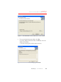
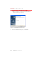


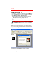

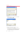
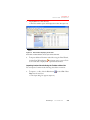
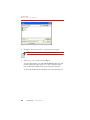


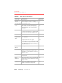


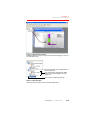
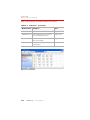
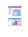
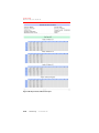


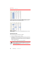
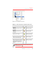
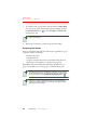
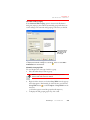
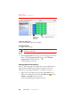

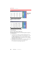

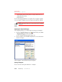
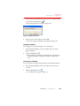
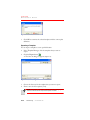
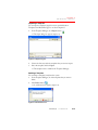


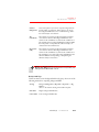
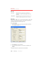
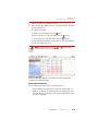
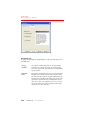
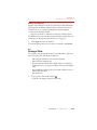


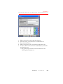


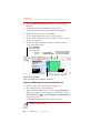
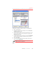

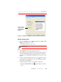
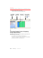


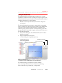

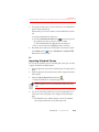
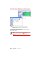

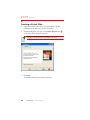
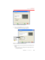
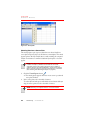
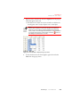


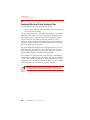
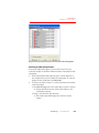
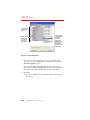

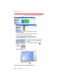
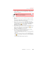

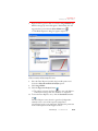


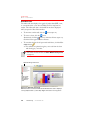

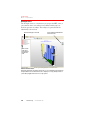

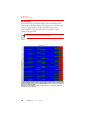

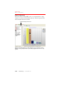


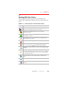


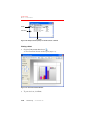

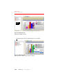


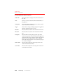


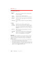

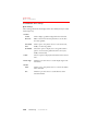


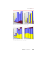

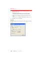


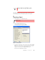
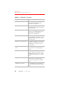
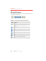
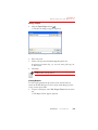
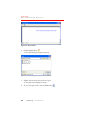


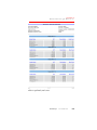

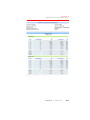
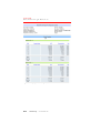
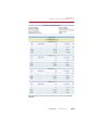


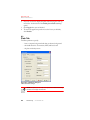


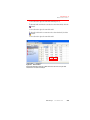

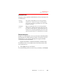


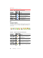

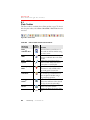


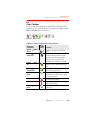
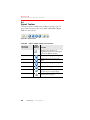
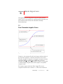
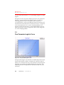
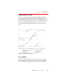
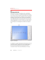
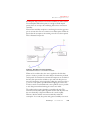
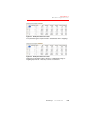

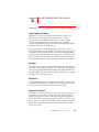


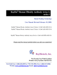
![or BTK [C481S] (cat. # CK-01-1002-384)](http://vs1.manualzilla.com/store/data/005787023_1-2d29b83e06663168d351d396f31f02d5-150x150.png)

![or BTK [C481S] (cat. # CK-01](http://vs1.manualzilla.com/store/data/005981492_2-10b1708324ced5982eb1bb254f0262a2-150x150.png)