1
By: Laurent Wismer & George Oner Water and Habitat Unit, International Committee of the Red Cross Nairobi regional Delegation Table of content 1. Introduction.......................................................................................................................1 First, a set of parameter must be set in the "main" worksheet. ................................................2 Second, the data must be entered or imported. Data are entered or imported worksheets that are mentioned right after. If data are imported, it is done with the importation tools................2 2. MAIN.................................................................................................................................2 3. NODES.............................................................................................................................5 3.1. Junctions ...................................................................................................................5 Base Data..................................................................................................................5 Additional Data ..........................................................................................................6 3.2. Reservoirs .................................................................................................................7 Base Data:.................................................................................................................8 Additional Data: .........................................................................................................9 Quality Data:..............................................................................................................9 3.3. Tanks.......................................................................................................................10 Base Data................................................................................................................10 Additional Data ........................................................................................................11 4. LINKS .............................................................................................................................11 4.1. Pipes........................................................................................................................12 Base Data................................................................................................................12 Additional Data ........................................................................................................14 4.2. PUMP ......................................................................................................................14 Base Data................................................................................................................14 Additional Data ........................................................................................................15 4.3. Valves ......................................................................................................................15 Additional Data ........................................................................................................16 5. VERTICES......................................................................................................................16 Base Data................................................................................................................17 Additional Data ........................................................................................................17 6. PATTERN AND CURVE.................................................................................................18 6.1. Pattern .....................................................................................................................18 6.2. Curve .......................................................................................................................18 7. CHART ...........................................................................................................................19 8. THE TOOLS MENU........................................................................................................19 8.1. Importation tools ......................................................................................................19 8.2. Exportation tools ......................................................................................................20 8.3. Organisation tools....................................................................................................20 8.4. Modification tools .....................................................................................................21 9. Surveying........................................................................................................................22 9.1. Surveying forms.......................................................................................................23 9.2. Surveying data.........................................................................................................24 10. Annexes............................................................................................................................1 10.1. UTM map ..............................................................................................................1 NSM 3 User Manual 14.09.2012 1. Introduction Network Survey Manager (NSM) is a database built on excel that can monitor, design and plot a water network. The information about this network can come from different sources, such as GPS/field surveying, GIS software or Epanet. Once this information has been managed by NSM, it can be exported to a GIS software, GPS, Epanet or Google Earth. The following figure shows an overall picture of the components that can be involved in NSM and their links. Create maps Make maps with the network Use GIS tools Check elevation profiles, find best path for pipes Desk study Place nodes on existing maps Field Collect Collect / complete data by unskilled staff Maps GPS Field Survey ArcView Import Txt from GPS fGIS Make Shp Import from Shp Map Source Make Gpx Excel Excel Import from old NSM NSM x.x Old versions NSM 3.7 Central DB for Water Networks Make Inp NSM 3.5 Tools Check data Sort IDs Rename IDs Round coord Calculate length Change Junction to Vertices Export options Make Kml Epanet Excel Google Earth Design Calculate flows & pressures NSM 3-7 manual 07-09-12.doc Easy use of data Calculate nb beneficiaries Prepare BoQ Adjust diameter according to PN Elevation profile 1/25 Visualisation Cross check with free Sat pictures LWI/GON NSM 3 User Manual 14.09.2012 When NSM is opened, many worksheets already exist and the worksheet "Main" is open. If trying to do a chronological sequence of the worksheets and tools that will be used, it would be like presented after. First, a set of parameter must be set in the "main" worksheet. Second, the data must be entered or imported. Data are entered or imported worksheets that are mentioned right after. If data are imported, it is done with the importation tools. The nodes in orange (junction, reservoir, tank), links in green (pipe, pump and valve) and vertices in pink are components of the network. They need to be filled in first. The pattern and curve in yellow are information about the water consumption of the community and the pump/tank/reservoir that will be used by the components of the network (for a pump or a junction with beneficiaries). They need to be filled in paralle to the nodes/links worksheet. However, given that some patterns and curves are already implemented, these worksheet might be used without being modified. Then data can be organised, modified and checked, using the organisation/modification tools and the "main" worksheet. The result can be seen in the chart worksheet, which is a chart of the network that is used at the end to visualise the network. Data can be exported with the exportation tools. To simplify the structure of this document, first the different worksheets will be presented, and then the tools. At the end, a detailed methodology of how to collect data from the field by surveying is given. 2. MAIN The main sheet is the control center of NSM. It is where the various NSM tools reside and is where the environment settings for the particular project network are set. In this section, only the settings will be discussed. The tool menu will be discussed in the tool section. NSM 3-7 manual 07-09-12.doc 2/25 LWI/GON NSM 3 User Manual 14.09.2012 Name of Project: This is where one enters the name of the network. No two networks should have the same name, else confusion will ensue. In cases where two or more networks are in the same locality, then a serial roman or alphabetical suffix should be used to differentiate them. For example Kandwi I, Kandwi II…. Kandwi N. Name of the project : Goma New Coordinate Bounds: This is a mitigatory measure to ensure that coordinates entered in the various sheets do not go beyond the target area. The bound coordinates should be the limit coordinates of the Minimum Bound Rectangle (MBR) around the network area. The Max(imum) X coordinate (E/W) is the Easting of the farthest edge of the network to the East, while the Min(imum) X Coordinate is the Easting of the farthest edge of the network to the West. The Max(imum) Y Coordinate is the Northing of the farthest edge of the network to the North while the Min(imum) Y is the Northing of the farthest edge of the network to the south. The Length refers to the number of digits that coordinate values should have Max X Coord (E/W) 750'000 Y Coord (N/S) 9'820'000 2'000 Min Decimals 741'500 1 9'812'000 1 1'460 1 Altitude Elevation Bounds: This is a measure against erroneous elevation entries. It sets the highest and lowest possible values acceptable as valid elevation entries. Please note that these checks only guard against obvious errors like missing a digit while entering values or adding an erroneous extra digit, or entering a value that would place your network feature outside the target area, BUT does not substitute ones caution and keenness to ensure that the values entered are correct. A wrong value that falls within the network MBR will not be detected. At the right of this table, the command button "Find min max" can find the maximum and minimum values, based on the data you entered in the sheet. This allows the opposite approach. It needs that data are first entered, and then the min and max are found. Based on these values, it can be determined if there is an erroneous data. Again, this will only detect obvious mistakes. WGS_1984 35 Coordinate System: A datum is a set of orientation, scaling and translation parameters applied to an ellipsoid of known physical parameters (major Axis, Minor Axis and Flattening) to best approximate the geoid. One is expected to understand the datum on which coordinates are declared for ease of data integration. Most of the time, the WGS 1984 is used. Once the datum is determined/selected, the topographical maps and GPS receivers being used in the field must be of or set to the selected datum. Datum UTM Zone M For standardization and ease of tools development, the projection is set to Universal Transverse Mercator (UTM) and all one has to set is the Zone in which the network lies. In case of difficulty, seek expert assistance. The table below can guide in the choice of zone if the longitude of the place is known. UTM Zone 1 2 3 Zone Range 180W - 174W 174W - 168W 168W - 162W NSM 3-7 manual 07-09-12.doc Central Meridian 177W 171W 165W UTM Zone 31 32 33 3/25 Zone Range 0E 6E 6E - 12E 12E - 18E Central Meridian 3E 9E 15E LWI/GON NSM 3 4 5 6 7 8 9 10 11 12 13 14 15 16 17 18 19 20 21 22 23 24 25 26 27 28 29 30 User Manual 162W 156W 150W 144W 138W 132W 126W 120W 114W 108W 102W 96W 90W 84W 78W 72W 66W 60W 54W 48W 42W 36W 30W 24W 18W 12W 6W - 156W 150W 144W 138W 132W 126W 120W 114W 108W 102W 96W 90W 84W 78W 72W 66W 60W 54W 48W 42W 36W 30W 24W 18W 12W 6W 0E 159W 153W 147W 141W 135W 129W 123W 117W 111W 105W 99W 93W 87W 81W 75W 69W 63W 57W 51W 45W 39W 33W 27E 21W 15W 9W 3W 34 35 36 37 38 39 40 41 42 43 44 45 46 47 48 49 50 51 52 53 54 55 56 57 58 59 60 14.09.2012 18E 24E 30E 36E 42E 48E 54E 60E 66E 72E 78E 84E 90E 96E 102E 108E 114E 120E 126E 132E 138E 144E 150E 156E 162E 168E 174E - 24E 30E 36E 42E 48E 54E 60E 66E 72E 78E 84E 90E 96E 102E 108E 114E 120E 126E 132E 138E 144E 150E 156E 162E 168E 174E 180W 21E 27E 33E 39E 45E 51E 57E 63E 69E 75E 81E 87E 93E 99E 105E 111E 117E 123E 129E 135E 141E 147E 153E 159E 165E 171E 177E As can be seen, there are 60 zones of 60 longitude belts which run serially from -1800 Longitude to 1800 Longitude. Similarly, there are 20 Sectors named serially in alphabetical order from C to X excluding I and O of 80 Latitude belts ranging from -800 latitude to +800 latitude. This is such that C-M and N-X represent the southern and northern hemispheres respectively. See the UTM zones and sectors for the whole below. When the square of interest is identified, first read the zone number of the column on the bottom of the map, and then the sector letter on the right. For Switzerland for example, it would give "32T". This map is put in a bigger format in the annexes. NSM 3-7 manual 07-09-12.doc 4/25 LWI/GON NSM 3 User Manual 14.09.2012 3. NODES These are the point features on the network. They signify the change in flow and flow characteristics, network outflows and inflows and network storage components. The nodes include Junctions, Reservoirs and Tanks. To fill in these worksheets, data can be imported using the importation tools (see the Tool Menu). 3.1. Junctions Junctions are points in the network where links join together or are changing their characteristics and where water enters or leaves the network. Hence a junction is when you have a T on a pipe, the end of the section, a house connection or change in the pipe’s diameter. For small networks, one can have a junction for every domestic point, while for large networks it might improve efficiency in calculation to model a series of domestic points using one junction with a demand equivalent to the combined demand. See example modelling below, where the corresponding series of domestic points and connections to the left are modelled into two nodes in the model to the right. Junction Vertices Figure 1 : Modelling domestic connections Base Data Base data Junction ID X-Coord Y-Coord Elev Demand J001 J002 742'933 742'746 9'815'965 9'815'745 1'490 1'490 5.29 3.97 Pattern paRural paRural Emitter X-Coord: This is the X- coordinate or the Easting of the junction. May be obtained using a GPS Receiver or scaled off a gridded topographic map. Ensure the GPS Receiver is set to the correct coordinate system, correct projection and correct geodetic datum (use UTM zones). T connection Houses XX 0.1 0.1 Junction ID: This is the unique identifier for the particular junction. Usually a serial sequence preceded by "J" to denote Junction for example J0001, J002, J003……..Jxxxn. Two Junctions should not have a similar ID. Description Bend JUNCTION Tee junction Blank end Y-Coord: This is the Y- coordinate or the Northing of the junction. Like with the X-Coord above, may be obtained using a GPS Receiver or scaled off a gridded topographic map. NSM 3-7 manual 07-09-12.doc 5/25 LWI/GON NSM 3 User Manual 14.09.2012 Please note that projection and datum is important to pay attention to, in this case if a GPS is used, the coordinate settings should be UTM. Check the "main" section. Elev: This is the elevation of the junction above mean sea level. Please note that this is NOT the elevation of the ground surface above mean sea level but rather that of the actual junction above sea level. Should the junction be buried d-metres below ground surface, then this must be subtracted from the height of the ground surface. Elevation can be approximated using the GPS (Please remember to indicate under description if this is the case) or interpolated from the grid contours, but most accurately through trigonometrical heighting or levelling. Demand: This refers to the outflow from the network at a particular junction. Only domestic points can have demand. The rest of the junctions have zero demand. In most cases, unless metre readings exist, demand is approximated from the beneficiary population. The number of people who are supplied from a particular junction, or the number of jerry cans that are drawn from the junction daily can be used to approximate the demand. It is described in Cubic Metres per Day. Pattern: This refers to the cycle of demand throughout the day. The regular behaviour pattern of the beneficiary population with reference to demand for water. What times of the day do more people draw the water and what times do one find fewer people. It is the variation of demand with time throughout the day. Example and useful patterns have been included within the pattern sheet of the NSM and one can select the most appropriate one. It can also be adapted by using the excel sheet "demand pattern" available in the annexes of the RefMan, under calculations. See pattern worksheet for more information Emitter: Emitters are devices associated with junctions that model the flow through a nozzle or orifice. In these situations the demand (i.e. the flow rate through the emitter) varies in proportion to the pressure at the junction raised to some power. Q s h exp onent They can be used to simulate leakage in a pipe connected to the junction (if a discharge coefficient and pressure exponent for the leaking crack or joint can be estimated) and compute a fire flow at the junction (the flow available at some minimum residual pressure). In the latter case one would use a very high value of the discharge coefficient (e.g., 100 times the maximum flow expected) and modify the junction's elevation to include the equivalent head of the pressure target. Description: This is for explanatory notes on any of the various data fields. Any information that is important but not captured by the existing data fields and any relevant remarks. Additional Data Additional data refers to all auxiliary data important in understanding the network but also clarifying base data. Some of it is redundant data to enable diagnose network calculation errors and data inconsistencies within the base data. However, if this information is available and relevant, it must be entered. It can simplify things in a couple of years, when the situation has changed and nobody is able to remember how it was before. NSM 3-7 manual 07-09-12.doc 6/25 LWI/GON NSM 3 User Manual 14.09.2012 State Date Installed Depth Ground Level Type Consumption Find Beneficiaries Additional info Comments Type: The type of junction it is. Whether T, L Y or Arrow junction. The find button will determine the type of junction it is, looking at the pipes that comes to that junction and go away from that junction. Beneficiaries: This is the number of beneficiaries who draw water from the junction. In the absence of water meter data, the demand at a junction, which is base data, is approximated from the number of beneficiaries using some standard indicators. For example 300 people relying on a domestic point could result in a demand of 15m3 per day assuming a standard water requirement of 50 litres per person per day. Y-Junction Arrow-Junction L-Junction T-Junction Consumption: This is the approximate daily consumption per person. In cases where an arrangement by the water committee and the community on the daily entitlement per person and/or household, this would be the figure reduced to the units of the number of people. Should you enter households instead of people in "No of People" column, the consumption must also be per household. One is however required to maintain consistency and in this case no of people and consumption per person should be adopted. Ground Level : (MASL) This is the height of the ground surface above mean sea level at the junction location. It is a working height from which you subtract the depth of the junction below ground to obtain the elevation in base data. Depth: (M) This the depth in metres of the junction below ground surface. Besides enabling you determine the actual elevation of the junction, is very important information about the junction during maintenance exercise. Date Installed: This is the date the junction was installed or the date of the last parts service (replacement). Important to determine serviceability and could be obtained from the office or from expert/experienced local knowledge. State: This is the state of repair of the junction. Whether it is very good, good, fair, poor or very poor. Comments: This is for explanatory notes on any of the various data fields. Any assumptions made, any information that is important but not captured by the existing data fields and any relevant remarks. 3.2. Reservoirs Reservoirs are the sources of water for the network. They are the inlet points through which water enters the network. They may be boreholes, wells, lake, dam, river intake among others. NSM 3-7 manual 07-09-12.doc 7/25 LWI/GON NSM 3 User Manual 14.09.2012 Please note that the spring is a special case as the discharge of water from the spring is independent of any downstream conditions within the network. As such, a spring is usually modelled as a junction with negative demand. The scalar part of the demand is the total flow discharge from the spring. Base Data: Base data Reservoir ID LacKivu1 LacKivu3 X-Coord 747'609 741'761 Y-Coord 9'813'174 9'815'633 Head Pattern 1'460.0 1'460.0 Description Captage Kivu Captage Keshero Reservoir ID: This is the unique identifier to identify the particular reservoir in the database. Like all the other components, every reservoir must have a unique identifier which as the name implies must not be similar to any other reservoir. Usually, a serial sequence prefixed with letter "R" as in R001, R002, R003………Rxxxn. However, since for most networks, the reservoirs are boreholes sometimes the prefix may be "BH" instead of "R". X-Coord: As is the case with the junction, and any other node for that matter, this is the XCoordinate or the Easting of the reservoir and can be obtained using GPS or by scaling off a topographic map with grid lines. Y-Coord: This is similarly the Y-Coordinate or the Northing of the reservoir and can be obtained using GPS or by scaling off a topographic map with grid lines. Head: As can be appreciated from the model above, the head is the height of the Dynamic Water Level (DWL) above mean sea level (or above adopted Datum). This can be obtained by determining the elevation of the ground surface then subtracting the DWL as is conventionally defined i.e. as a depth from ground surface. NSM 3-7 manual 07-09-12.doc 8/25 LWI/GON NSM 3 User Manual 14.09.2012 Pattern: This is the variation of the Dynamic water level with time. If this is possible to obtain, should be included otherwise, time should not be lost looking for it as it is not too critical. Description: This is for explanatory notes on any of the various data fields. Any assumptions made, any information that is important but not captured by the existing data fields and any relevant remarks. Additional Data: State Date Installed Depth Protected Yield l/d Type Ground Level Additional info Comments The Ground Level (m), Depth, Date Installed, State and Comments are as explained under Junctions. Type: This is whether the reservoir is a borehole, a River Intake, a Dam, a well, a lake or a connection to another supply network. Yield l/d: this is the maximum discharge the source can sustain in litres per day Protected: Whether the water source is protected or not. Please indicate in the description what kind of protection it is. Quality Data: This is for information about the quality of water from the source. Whichever method is used to determine the quality parameters must be described under the description column. Please note that water quality is a sensitive issue especially in public water supply and must be handled in a cautious manner. Conductivity Colour Turbidity PH Quality CommentsQ pH: The pH of a sample of water is a measure of the concentration of hydrogen ions. It is the negative logarithm of the hydrogen ion (H+) concentration. What this means is that at higher pH, there are fewer free hydrogen ions, and that a change of one pH unit reflects a tenfold change in the concentrations of the hydrogen ion. For example, there are 10 times as many hydrogen ions available at a pH of 7 than at a pH of 8. The pH scale ranges from 0 to 14. A pH of 7 is considered to be neutral. Substances with pH of less that 7 are acidic; substances with pH greater than 7 are basic. Since pH can be affected by chemicals in the water, pH is an important indicator of water that is changing chemically. This value is obtained either at a water testing laboratory or using a pH meter. NSM 3-7 manual 07-09-12.doc 9/25 LWI/GON NSM 3 User Manual 14.09.2012 Turbidity (NTU): This is the amount of particulate matter that is suspended in water. Turbidity measures the scattering effect that suspended solids have on light: the higher the intensity of scattered light, the higher the turbidity. Turbidity is measured in NTU (nephelometric turbidity units). May be measured in a laboratory or using a handheld turbidity meter. Colour (mgPt/l): This is a visual interpretation of the colouration in water. If tested in a laboratory would be measured in mgPt/l, but visually interpreted as greenish, brown or no colour among others. Conductivity (µS/cm): Electrical conductivity (EC) estimates the amount of total dissolved salts (TDS), or the total amount of dissolved ions in the water. It is measured in micro Siemens per centimetre (µS/cm). CommentsQ is like in the other cases used to record any relevant remarks, assumptions or extra information. 3.3. Tanks These are storage systems used to retain water for distribution in periods when pumping or extraction from the reservoir is not on-going. They are like buffer systems to regulate flow at the distribution end. Diameter Overflow Inlet Max level Outlet Initial level Min level Figure 2 : Tanks modelling Base Data Base data Tank XYElevatio Init Min Max Min Vol Diameter ID Coord Coord n Level Level Level Vol Curve TBush 749'042 9'819'024 a 1'619 1.5 0 3 23 Description Nouveau Tank ID: This is the unique identifier to identify the particular storage tank in the database. Like all the other components, every tank must have a unique identifier which as the name implies must not be similar to any other tank. Usually, a serial sequence prefixed with letter "T" as in T001, T002, T003………Txxxn. X-Coord and Y-Coord are as explained under Junctions and Reservoirs NSM 3-7 manual 07-09-12.doc 10/25 LWI/GON NSM 3 User Manual 14.09.2012 Elevation: As shown on the model, elevation is the height of the tank-bottom above mean sea level. Since most of the times they are elevated tanks, this may be obtained by determining the height of the ground surface and adding the height of the tank-base above ground. Initial Level: This is the height of water surface above tank-bottom in metres at the start of network calculation. In other words, the length of water column within the tank at the start of network calculation/analysis. Min Level: This is the level of water in tank in metres below which there is no possibility for water to leave the tank. It is the height of the outlet pipe from the base of the tank. Max Level: This is the maximum height in metres water can attain above the tank base. Usually the height of the overflow pipe from the base of the tank. Diameter: The diameter of the tank in meters. For cylindrical tanks this is the actual diameter. For square or rectangular tanks it can be an equivalent diameter equal to 1.128 times the square root of the cross-sectional area. For tanks whose geometry will be described by a curve (see VolCurve) it can be set to any value. Min Vol: The volume of water in the tank when it is at its minimum level, in cubic meters. This is an optional property, useful mainly for describing the bottom geometry of noncylindrical tanks where a full volume versus depth curve will not be supplied (see next). Vol Curve: The ID label of a curve used to describe the relation between tank volume and water level (see Volume curve under the curve worksheet). This property is useful for characterizing irregular-shaped tanks. If left blank then the tank is assumed to be cylindrical. Description: any other relevant data Additional Data State Date Installed Height Type Ground Level Additional info Comments Height: this is the height of the tank All other additional data are as explained in the junctions and reservoirs. 4. LINKS These are the edge features on the network. They convey the water between nodes in the network and comprise of Pipes, Pumps and Valves. Again, to import data to fill in these worksheet, see the importation tools (in the Tool Menu) NSM 3-7 manual 07-09-12.doc 11/25 LWI/GON NSM 3 User Manual 14.09.2012 4.1. Pipes Base Data Base data Find Pipe ID Node 1 Node 2 Length Diamet Roughn MinorL Status Description er ess oss Pipe ID: A unique identifier for the particular pipe. Usually a serial sequence with prefix letter "P" as in P001, P002, P003………Pxxn Node 1: The ID of the upstream node, which could be a junction, a reservoir or a tank. The Identifier of the start point of the particular pipe. Direction of flow Node 1 Node 2 Node 2: The ID of the downstream node, which could be a junction, a reservoir or a tank. The Identifier of the end point of the particular pipe. Length: This is the length dimension of the pipe in "m" and can be calculated if all the necessary vertices are included in the survey and database, else should be measured and manually entered Diameter: This is the internal diameter of the pipe in "mm" Roughness: The roughness coefficient of the pipe. It is Darcy-Weisbach roughness and has units of mm. Material Concrete or Concrete Lined Galvanized Iron Plastic Steel Asbestos cement New Pipe 0.300 - 0.700 0.100 - 0.150 0.001 - 0.002 0.020 - 0.060 0.030 - 0.100 Old Pipe 0.100 - 3.000 0.200 - 0.500 0.100 - 0.500 Minor Loss: Losses occur in straight pipes and ducts as major loss and in system components as minor loss. Components as valves, bends, tees add head loss commonly termed as minor loss to the fluid flow system. NSM 3-7 manual 07-09-12.doc 12/25 LWI/GON NSM 3 User Manual 14.09.2012 Below is a table of minor loss coefficients for a variety of network components Type of Component or Fitting Minor Loss Coefficient - K Tees: Flanged, Line Flow 0.2 Threaded, Line Flow 0.9 Flanged, Branch Flow 1.0 Threaded, Branch Flow 2.0 Threaded Union 0.08 Elbows: Flanged Regular 90o 0.3 o Threaded Regular 90 1.5 o Threaded Regular 45 0.4 o Flanged Long Radius 90 0.2 o Threaded Long Radius 90 0.7 o Flanged Long Radius 45 0.2 o 180 Return Bends: Flanged 0.2 Threaded 1.5 Valves: Fully Open Globe 10 Fully Open Angle 2 Fully Open Gate 0.15 1/4 Closed Gate 0.26 1/2 Closed Gate 2.1 3/4 Closed Gate 17 Forward Flow Swing Check 2 Fully Open Ball 0.05 1/3 Closed Ball 5.5 2/3 Closed Ball 200 Pipe Entrance (Reservoir to Pipe): Square Connection 0.5 Rounded Connection 0.2 Re-entrant (pipe juts into tank) 1.0 Pipe Exit (Pipe to Reservoir): Square Connection 1.0 Rounded Connection 1.0 Re-entrant (pipe juts into tank) 1.0 hminor_loss = ξ v2/ 2 g (1) where hminor_loss = minor head loss (m) ξ = minor loss coefficient v = flow velocity (m/s) g = acceleration of gravity (m/s2) Status: Whether the pipe is Closed, Open or is fitted with a Check Valve. Check valves are two-port valves, meaning they have two openings in the body, one for fluid to enter and the other for fluid to leave. Could be gate or non-return valves NSM 3-7 manual 07-09-12.doc 13/25 LWI/GON NSM 3 User Manual 14.09.2012 Additional Data State Thickness Date Installed Find External Diameter PN Material Additional info Comments Material: This is the material of the pipe such as GI, PVC, Steel etc. It is important to understand the derivation of the absolute roughness values PN: This is the nominal pressure of the pipe. It indicates the maximum working pressure for a pipe. External Diameter: This is the diameter of the exterior ring surface of the pipe Thickness: This is the difference between the internal and external diameters. It is the incident perpendicular distance from the centre of the pipe that is in contact with the pipe material. The command "find" will return a thickness based on the material and the PN. For this command to work, the material and PN must be put as indicated in the comment relative to their column (for example, for the nominal pressure, it must be written PN10 and not 10). If the material is different than the one proposed in the comment of material, it will return "Mat unknown". The date installed and State and Comments are as discussed in the earlier instances. 4.2. PUMP Base Data Base data Pump ID Node 1 Node 2 PumpCurve Pattern Description Pump ID: A unique identifier for the particular pump. Usually a serial sequence with prefix letters "Pu" as in Pu001, Pu002, Pu003………Puxxn Node1 & Node 2 are as explained under pipes except that Node1 is usually a reservoir PumpCurve: It is the combination of heads and flows that the pump can produce. A Pump Curve represents the relationship between the head and flow rate that a pump can deliver at its nominal speed setting. Head is the head gain imparted to the water by the pump. A valid pump curve must have decreasing head with increasing flow. NSM 3-7 manual 07-09-12.doc 14/25 Junction Pump Reservoir LWI/GON NSM 3 User Manual 14.09.2012 Additional Data Date Installed Model No Type Power kVA Additional info State Comments Type: What type of pump it is. Usually the manufacturer and the operational mode Power (kVA): This is the power rating of the pump. Model No. The model Number as issued by manufacturer or any existing industry standards The Date Installed, State & Comments are as already described in earlier chapters (see Junctions or Reservoirs) 4.3. Valves Valves are used to control the pressure or flow at a specific point in the network. Shutoff (gate) valves and check (non-return) valves, which completely open or close pipes, are not considered as separate valve components but are instead included as a property of the pipe in which they are placed Base data NSM 3-7 manual 07-09-12.doc 15/25 LWI/GON NSM 3 Valve ID User Manual Node 1 Node 2 Diameter Type Setting MinorLoss 14.09.2012 Description Valve ID: A unique identifier for the particular valve. Usually a serial sequence with prefix letter "V" as in V001, V002, V003………Vxxn Node 1 and Node 2 are as described under pipes. Diameter: The diameter of the valve Type: This is the type of valve. Only six possible entries can be made and these are PRV(Pressure Reducing Valve), PSV(Pressure sustaining Valve), PBV(Pressure Breaking Valve), FCV(Flow Control Valve), TCV(Throttle Control Valve) or GPV(General Purpose Valve). Please note it is the abbreviations only. Most common networks do not have these valves and one has to be really sure of the valve before indicating it as a valve. Most valves encountered are NRV (Non Return Valves), air valves and gate valves that are not classified as Valves in this case but included in then properties of the pipes. Setting: A required parameter that describes the valve's operational setting. Valve Type Setting Parameter PRV PSV PBV FCV TCV GPV Pressure (m) Pressure (m) Pressure (m) Flow (flow units : m3/h) Loss Coeff. (unitless) ID of head loss curve Minor Loss: is a Unit less minor loss coefficient that applies when the valve is completely opened. Assumed 0 if left blank. For further explanation of the minor loss, see under pipes. Additional Data Additional info Material Date Installed State Description The additional information fields are as explained in the previous chapters (see under pipes) 5. VERTICES These are points along links where there is a change in alignment but which are not junctions or any other node for that matter. Where the link direction changes probably for no flowrelevant reason but to probably keep the network alignment within the acquired easements NSM 3-7 manual 07-09-12.doc 16/25 LWI/GON NSM 3 User Manual 14.09.2012 or to avoid obstacles or for any reason whatsoever not linked to the flow system. The vertex data structure can be used to document such network components like elbows, air valves, gate valves, NRVs among others which would otherwise be missed within the other databases. There is sometimes the tendency not to use this option and Bend put a junction instead of a vertex. Nevertheless, it simplifies things and is therefore advisable to put a vertex when relevant. It will be seen after that a tool exists to transform a junction into a vertex (see modification tools in the tools menu). VERTICE Base Data Tee junction Base data Link ID (pipe) X-Coord Blank end Y-Coord Reducer Link ID: This is the link on which the vertex lies. It must be an ID which is already entered either under Pipes(the most usual and expected), valves or Pumps. X-Coord & Y-Coord are as explained under the various node components. See under junctions. Additional Data Elev Ex ID Description Type GL Depth Date Installed Additional info State Comments Elev, Depth, Date installed, State and Comments are as explained under the junctions section. Ex ID: This the previous ID. It is used when a junction is transformed into a vertex, with the tools junction to vertex. Otherwise, it is left blank. Description: one could be able to indicate whether the node is a NRV, Gate Valve, Air Valve or whatever kind of structure. Type: Here can be put a particularity of the vertex (for example if it is an elbow, a high-point or a low-point) GL: Ground level, as it was explained in the previous worksheets. NSM 3-7 manual 07-09-12.doc 17/25 LWI/GON NSM 3 User Manual 14.09.2012 6. PATTERN AND CURVE 6.1. Pattern This information will be used in a junction with a certain number of beneficiaries that will take water or in a reservoir or a pump. This refers to the cycle of demand throughout the day. The regular behaviour pattern of the beneficiary population with reference to demand for water. What times of the day do more people draw the water and what times do one find fewer people. It is the variation of demand with time throughout the day. It is expressed in percentage or fraction of the average hourly consumption. Thus, an hour that has a fraction greater than one, means that the consumption is greater in that hour than the daily consumption divided by 24 hours, and the other way around. The average of this fraction or percentage should be 1 or 100% respectively. Here, some examples of pattern have been put. Varying demand Demand 0 1 2 3 4 5 6 7 8 9 10 11 12 13 14 15 16 17 18 19 20 21 22 23 Pattern 0.1 0.1 0.1 0.1 0.3 1.0 1.9 2 2.0 1.9 1.5 1.1 1.0 0.9 1.1 1.8 2.0 2.0 1.5 1.0 0.3 0.1 0.1 0.1 Constant demand throughout daylight Demand 0 1 2 3 4 5 6 7 8 Pattern 0 0 0 0 0 0 2 2 2 9 2 10 11 12 13 14 15 16 17 18 19 20 21 22 23 2 2 2 2 2 2 2 2 0 0 0 0 0 0 Constant demand throughout the day Demand 0 1 2 3 4 5 6 7 8 Pattern 1 1 1 1 1 1 1 1 1 9 1 10 11 12 13 14 15 16 17 18 19 20 21 22 23 1 1 1 1 1 1 1 1 1 1 1 1 1 1 Example and useful patterns have been included within the pattern sheet of the NSM and one can select the most appropriate one. For example the pattern may be indicated as "paFlat", "paOnOFF" or "paVillage". It can also be adapted by using the excel sheet "demand pattern" available in the annexes of the Reference Manual, under calculations. 6.2. Curve This worksheet stores information about some data that are used in other worksheets. It is data that have two variables that are linked together (the change of one variable will affect the other). If a graph is done as one variable versus the other, it would form a curve. In this worksheet, the goal is not to put the equation of the curve, but only to put some points (with the value of the two variables it depends from) and the program will extrapolate the value in between these points. The more points are put, the more precise the result will be. Pump This curve will be used in the pump worksheet. A Pump Curve represents the relationship between the flow rate in m3/h (in x) and the head in m (in y) that a pump can deliver at its nominal speed setting, where the head is the head gain imparted to the water by the pump. On pumps booklets furnished by the supplier, the characteristic curve of the pump is put. A valid pump curve must have decreasing head with increasing flow. Volume It is used in the tank worksheet. This property is useful for characterizing irregular-shaped tanks. For a cylindrical tank, there is no need to create a curve, since when the section VolCurve is left blank it is assumed that the height is directly proportional to the volume. If NSM 3-7 manual 07-09-12.doc 18/25 LWI/GON NSM 3 User Manual 14.09.2012 this is not the case, some height in m (in x) and corresponding volume in m3 (in y), should be put. Efficiency This refers to the efficiency of a pump, in function of the flow. Indeed, a pump will have varying efficiencies, depending on the flow it pumps. The efficiency will be maximal when the pump works at its nominal point. The efficiency can be used to estimate the power consumption of the pump. Put the flow in m3/h (in x) and the corresponding efficiency in % (in y). Headloss This is used in the valve worksheet, when working with a GPV. The headlosses are function of the flow. Put the flow in m3/h (in x) and corresponding head loss in m (in y). 7. CHART In this worksheet, a 2-D representation of the network is drawn. This might not be sufficient to allow to visualise the network in the space. Therefore, the data can be exported to a GIS software or Google Earth (see exportation tools). It could also be exported to a GPS, to check on the field how it would look like. As mentioned before, the data can be exported towards Epanet to make further calculation on the design. 8. THE TOOLS MENU The tools can either be found on the toolbar (that will be seen from all worksheets), or, for some of them on the "main" worksheet. The tools that have a command on the "main" worksheet can be used from whatever worksheet, because it will affect all sheets; however, it usually makes sense to use this command from the "main" worksheet (especially for "check worksheets" whose result will be shown on the "main" worksheet). For the other tools, they have to be used from another sheet, because they will only modify the sheet that is open, and will not change the other (for example sort worksheet). Tools available form the "main" worksheet toolbar 8.1. Importation tools Import from Old NSM: This tool enables backward compatibility. As NSM undergoes evolution, data created in the previous versions would require too much time to convert to the NSM 3-7 manual 07-09-12.doc 19/25 LWI/GON NSM 3 User Manual 14.09.2012 current version. This tool enables all such data to be automatically imported and converted to the current version. Import from Shp: Import Nodes data from point shape files (i.e. GIS software), preferably with the same format. Can only be used from a nodes/vertices worksheet. Import vertices from pipes: this will import the vertices of a pipe that is stored as a polyline in a shapefile. This tool can only be used from the vertex worksheet. Import Inp from Epanet: this tool will import data from an Epanet project. Be aware that when using this tool, all data in the workbook will be erased. Import txt from GPS: Import Nodes data from a txt file generated by MapSource. This enable you to get data collected with a GPS, and cleaned with MapSource. It is usually easier to make several files for different kind of nodes (especially when there are a lot of data) and import them one file after another from different worksheets, in order not to have to change manually the worksheet in which the node is put. 8.2. Exportation tools Make Shapefiles: This tool exports your NSM database into corresponding set of ESRI format shapefiles consisting of all the network components. In the latest version of NSM, a projection file is included for every shapefile to alert the applications interacting with the shapefile on the projection of the shapefile data. Make inp File: This tool export the network into a ready Epanet (.inp) file which can be calculated and analysed by Epanet. Make kml File: This tool export the network components into the Keyhole Markup Language (kml) format which can be viewed directly in Google Earth. Make Gps File: This tool export data into a .txt file that can be loaded on a GPS device. 8.3. Organisation tools Hide / Show Surveying Data: For all nodes, links and vertices, the first columns are information concerning surveying. This information is not always relevant (for example if the information on the nodes/links does not come from a surveying); therefore, there is the possibility to hide these first columns when they are not needed. NSM 3-7 manual 07-09-12.doc 20/25 LWI/GON NSM 3 User Manual 14.09.2012 Check Worksheets: This tool is used to verify the validity of data entered in the various sheets, especially the base data. Sheet Records ID Check Base Data columns Col Col Col Col Col Col 3 Col 4 2 5 6 7 8 Junction Reservoir Tank 10 1 1 OK OK OK OK OK OK OK OK OK OK OK OK OK OK Pipe 11 OK OK OK OK Pump Valve Vertice Pattern Curve Total 0 0 0 13 10 5 OK OK OK OK OK OK OK OK OK OK OK OK OK OK OK OK OK OK OK OK OK OK OK OK OK OK OK OK OK OK OK OK Lonely or not existing nodes It looks out for invalid entries, such as type mismatch, unknown/non-existent component IDs, lonely components and missing data. Straight away the data errors can be singled out and corrected without having to encounter errors in running the other functional tools. The result of this check is given in a table in the "main" worksheet. Sort Worksheet: This will sort the worksheet alphabetically based on their ID. Be aware that for example 15 is sorted before 5 (because it looks first at the first number); therefore, in order to be able to use this command in a wise manner the ID should be written with zeros in front (for example 003 instead of 3, the numbers of zeros depends on the number of points that are expected). It will be seen after that there is a tool that allows to rename IDs automatically (see the Rename ID tool). In order to use this function, you have to be on the worksheet you want to change. 8.4. Modification tools Round All Coordinates: This is purely for data precision integrity. It rounds off the coordinate values to whole numbers. The technologies currently used to determine the coordinates (GPS & scaling from topo map) cannot yield sub-meter precision. Calculate Pipe Length: This tool calculates the 3-D length of the pipe where the length does not already exist. Please note that the length will only be correct if the best-fit alignment vertices are observed and included in the database. Rename ID: this gives the possibility to rename systematically your ID. Again this option only works if it is used in the workbook to be modified. By clicking on it, this kind of window will appear. It has different possibilities (three thumbnail). The first is "single", in which it is possible to change the ID one by one, by choosing the ID to be changed and defining a new ID. The second is "Batch Add". This will automatically change the ID of all nodes that have only a NSM 3-7 manual 07-09-12.doc 21/25 LWI/GON NSM 3 User Manual 14.09.2012 numerical ID (this means that an ID that has letters in it would not be changed). It is possible to add a letter in front of the ID (for example j for junction), and to define the wanted number of digits, by clicking in front of the number of # that is wanted. Example Letter to add: J Number of digits: ### (3 digits) If an ID is named 5 before, it would be changed to: J005 If an ID is called J5, it will not be changed (since it is not only numerical). The third thumbnail is "Remove Batch", which allows to remove a specific letter/group of letters in front of all ID. Junction to Vertice: This gives the possibility to change a junction to a vertex. Indeed, it can simplify the network to have vertices instead of junctions when relevant (no pipes attributes changes and no demand). NSM will check if some junctions could be transformed into vertices and ask if it want to be changed. Erase All Data: This tool enables rapid refresh when a new network database is to be created. All sheets are reset to empty and a new network can then be built from scratch. Be careful to use this tool as it could erase data that you still need. Options: With this command, some settings can be chosen. First, under the thumbnail "main", the settings that will be used when checking the worksheets can be defined (for example, the maximum number of connections at a node). The thumbnails "KML", "Epanet" and "GPX", some options can be chosen that will be used when exporting the data to these formats. For example, under "Epanet", the unit of the flow can be chosen (whether it is in liters/min of in cubic meters/hours and so on). 9. Surveying As it was already mentioned in the introduction, there are many ways of collecting your data. One of these ways is the field approach with topological surveying, which is described in more details in this section. Storage / Treatment Strainer Source Pump Distribution Figure 3 : Actual situation The survey involves a systematic sketching of a network alignment and its components, positioning the alignment vertices, the network components and naming the various components and vertices. The sketching may be done on a topographic map of the area if available or on pure plain sheet. The components are symbolized and annotated in the sketch systematically and such annotations used to fill the survey part of the field data collection sheet. NSM 3-7 manual 07-09-12.doc 22/25 LWI/GON NSM 3 User Manual 14.09.2012 The positioning here refers to determination of coordinates for every important point in the network. It may be done by scaling off the topographic map or by using the GPS receiver. Since different GPS receivers could be used by different teams to carry out survey of the same network, it is important to identify the field officer, the GPS receiver used, the Map Sheet used and the date of survey. Field Officer GPS Receiver ID Date Map Sheet ID An example survey process to document the simple network above would proceed as follows: Figure 4 : Sketch the network As can be seen the network components are symbolized and annotated. The annotations are made simple so as to enable easy field work. The numbers are the serial numbers as obtained from the GPS receiver. The m2,m3,m4 are points which could not be taken by GPS for one reason or the other and are only marked on the topographic map. As can be seen, 10 is a reservoir, 11 is a junction, m2 is a tank, 12 and m3 are vertices and13-16 and m4 are junctions. The details are then entered into the relevant forms 9.1. Surveying forms JUNCTION, VALVES & INTERMEDIATE NODES FORM Depth (m) Confirmed (Y/N) ID Location State (P,F,G,U) GPS Position No. Functioning (Y/N) Pipe_TO Locality Type (J,V,IN etc) Pipe_From Type_Size (mm) Map Position No. Description Elevation Demand Curve No. No. of People Consumption l/p/d Total Demand L RESERVOIR FORM Type (Well,BH,,RWC etc) ID Yield (Litres/Day) Confirmed(Y/N) GPS POSITION NO. Location MAP POSITION NO: Power PUMP Pump (Y/N) Type Pump_Level Model_No Connected(Y/N) Permanent(Y/N) QLow QDesign QMax HLow HDesign HMax Description NSM 3-7 manual 07-09-12.doc 23/25 LWI/GON NSM 3 User Manual Approximate Confirmed Water Level Static Protected(Y/N) State (P,F,G,U) pH (pH Scale) Turbidity (NTU) Elevation Quality 14.09.2012 Dyna. T1 Dyna. T2 Description: Colour (mgPt/l) Conductivity (µS/cm) TANK FORM Elevation Min Volume Volume Curve Present Level Minimum Level Maximum Level Date_Installed Diameter ID GPS Position No. Location Pipe_To Pipe_From Map Position No. Description LINK (Pipe, Pump, Valve & Intermediate Node) FORM Type (Pi,Pu,V,IN) ID GPS Position No. Location PUMP/ VALVE Power/ Setting Node1 (N1) Pu/V Type Node2 (N2) Model No. Date_Installed QLow QDesign HLow HDes Diameter (mm) QMax HMax Material Map Position No. Description The data from the forms are entered into the database. They are categorized as Surveying Data, Base Data and Additional Data. For water sources (Reservoirs), the quality data is also a category. The survey data is common for all network components, while the base and additional data very from component to component. See further descriptions below. 9.2. Surveying data F01 Mhd Ali 12.10.08 Z1 Date GPS ID P08 136 137 138 Map Pos No Field O GPS pos No Form Index Map ID Surveying data Locality District Juncti on ID Dema nd Pattern 136 Kandwi Micheweni 137 M01 138 This is the information input so as to document knowledge about the survey exercise. It comprises of information about the persons doing the survey work, the instruments used, the date of survey, the area in which the survey takes place and importantly, the field collection sheet used to record field data. Form Index: This is the index Number of the form used to record field data. Field Data Collection Forms are serialised/Indexed to enable easy identification and to aid trace-back in case of wrong entries or any other sort of human error NSM 3-7 manual 07-09-12.doc 24/25 LWI/GON NSM 3 User Manual 14.09.2012 Field Officer: This is the name of the field officer who carried out the field survey Date: The date on which the field data was collected GPS ID: The Identification Number for the GPS Receiver used to collect the coordinates of the specific network feature. As the project could employ the use of a number of GPS receivers, it would be useful in determining which one was used for ease of traceability and data verification Map ID: In some instances, the field team does not have a working GPS, in which case a 1:10000 topo sheet section printout will be used to mark the location of the network point feature. This field enables the field team to document which map sheet was used to mark the position GPS Pos No: Within the GPS Receiver memory, sometimes the point locations are stored using the automatically generated serial numbers. In other cases, though cumbersome, one may be able to fully type out the name of the point feature. This column documents the serial number of the point feature within the GPS Receiver memory Map Pos No: The identity used to mark the position of a network point feature on the topo sheet printout. Locality: The village or area in which the survey is carried out. For most networks, this is usually the name of the network, but not always. For some networks, which stride various localities, it is important that the actual locality where the feature lies is indicated. District: This is the administrative district in which the feature lies. NSM 3-7 manual 07-09-12.doc 25/25 LWI/GON NSM 3 10. User Manual 14.09.2012 Annexes 10.1. UTM map NSM 3-7 manual 07-09-12.doc 1/1 LWI/GON