Download Depth estimation with the matched filter (C03)

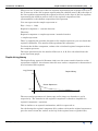
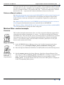
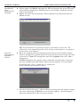
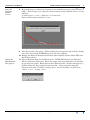
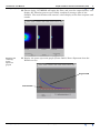
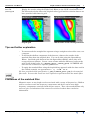
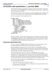
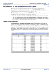
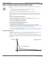
INTREPID User Manual
Library | Help | Top
Depth estimation with the matched filter (C03)
1
| Back |
Depth estimation with the matched filter (C03)
Top
This chapter describes two approaches to depth estimation that use the matched
filter:
•
Separation filtering as described by Cowan and Cowan (1993)
•
Depth slicing as described by Norman (1993)
Spector and Grant (1970) provide a foundation for these techniques.
This method uses the power spectrum graph of a magnetics grid in the spectral
domain. Magnetic sources at similar depths show straight-line segments in this
graph.
Location of sample data for Cookbooks
Where install_path is the path of your INTREPID installation, the project
directory for the Cookbooks sample data is
install_path\sample_data\cookbooks.
For example, if INTREPID is installed in
C:\Program Files\Intrepid\Intrepid4.5,
then you can find the sample data at
C:\Program Files\Intrepid\Intrepid4.5\sample_data\cookbooks
For information about installing or reinstalling the sample data, see "Sample data for
the INTREPID Cookbooks" in Using INTREPID Cookbooks (R19).
For a description of INTREPID datasets, see Introduction to the INTREPID database
(G20). For more detail, see INTREPID database, file and data structures (R05).
Separation filter theory
This method assumes that you can summarise the power spectrum in terms of two
straight line segments, characterising the regional and shallow sources.
The slope of a line segment indicates the depth of the sources that it characterises.
The intercept with the vertical axis is an indication of the intensity of the source at
that depth.
Log (Power)
Separation Filter
B
Power Spectrum
b
Wavenumber
Library | Help | Top
© 2012 Intrepid Geophysics
| Back |
INTREPID User Manual
Library | Help | Top
Depth estimation with the matched filter (C03)
2
| Back |
Where B is the Y intercept of the line segment representing the regional sources;b is
the Y intercept of the line segment representing the shallow sources;H is the slope of
the line segment representing the regional sources;h is the slope of the line segment
representing the shallow sources.A1(r) is the regional component of the
spectrumA2(r) is the shallow component of the spectrum
You can represent the complex spectrum as
E(r) = A1(r) + A2(r)
Regional component = transfer function
Therefore
Regional component = complex spectrum / transfer function
= complex spectrum.
Thus, by applying the transfer function to the complex spectrum, you can obtain the
regional component. The matched filter performs this operation.
To obtain the shallow component, subtract the calculated regional component from
the complex spectrum.
The input parameters for the matched filter are b, h, B, H as calculated from the
power spectrum graph
Depth slicing theory
The depth slicing approach (Norman 1993) uses the same transfer function as the
separation technique, but assumes that the near surface component is characterised
by a horizontal line segment.
Log (Power)
Depth Slicing
B
Power Spectrum
b=1
Wavenumber
The near surface parameters b (intercept) and h (slope) are therefore 1 and 0
respectively. The formula for the regional component is therefore simplified to
regional component = spectrum .
This is similar to an upward continuation, which is expressed as
On calculating the regional component (D1), subtract it from the original spectrum to
give the sources from the surface to the top of the regional sources (product S1).
Library | Help | Top
© 2012 Intrepid Geophysics
| Back |
INTREPID User Manual
Library | Help | Top
Depth estimation with the matched filter (C03)
3
| Back |
You can repeat the process on product S1 to produce a deep component (D2). subtract
the D2 from S1 to give a shallower set of solutions (product S2). You can repeat the
process a number of times. The products D1, D2, ... represent 'depth slices' and the
products S1, S2, ... represent the residual (shallower) sources in each case.
Reference Manual sections
See"Querying the power spectrum graph (OldGridFFT)" in Old spectral domain grid
filters (OldGridFFT) (T38) for instructions on obtaining the Spector-Grant filter
depth estimate, intercept and slope for a straight line segment in a grid’s power
spectrum.
See "Matched filter (reference)" in INTREPID spectral domain operations reference
(R14) for general information about the matched filter in INTREPID.
See "Matched Filter (OldGridFFT)" in Old spectral domain grid filters (OldGridFFT)
(T38) for instructions on using this filter with grids.
Matched filter—worked example
Overview
This worked example demonstrates the use of the separation filtering approach for
extracting the regional component of a survey. You will use the Spectral Domain
Grid Filter tool. You will use the power spectrum graph of a grid dataset to calculate
intercept and slope for two line segments representing the regional and shallow
sources. You will then apply a matched filter with these parameters to the grid
dataset and examine the results.
Steps to follow
Start S D Grid
Filters; Specify
input and
output datasets
Library | Help | Top
1
In the INTREPID Project Manager locate the Cookbook interpretation data
directory (e.g., d:\intrepid\sample_data\cookbooks\interp_min).
2
Start the Spectral Domain Grid filters tool (FFT_Filter from the Filtering menu)
3
Specify mlevel_grid as the Input Dataset. Specify an Output Dataset (You
must output to the grid match_grid1 if INTREPID is running in demonstration
mode. We provide an identical solution dataset for you to compare called
match_grid). Accept the default forward and reverse FFT options as displayed
in the corresponding dialog boxes.
© 2012 Intrepid Geophysics
| Back |
INTREPID User Manual
Library | Help | Top
Calculate the
power
spectrum; View
the graph
Query the
graph for deep
(regional)
sources
Depth estimation with the matched filter (C03)
4
| Back |
4
Choose Apply. INTREPID will apply the FFT and generate the power spectrum
for the dataset, displaying a ‘Filtering process successfully completed’ message
when it has finished.
5
Display the power spectrum graph. (Choose Radial Power Spectrum from the
Window menu).
6
Tip: The horizontal axis represents frequency of the data in cycles/km. The
vertical axis is the natural logarithm of the energy at that frequency, averaged for
all directions in the dataset.
Query the graph for the deep (regional) sources Spector-Grant depth estimate.
Locate a straight line segment in the low frequency (deep source) range and click
each end of it. Note: The straight line must be a segment of the curve, not a
tangent to it.
INTREPID displays the segment using a white line and report the Y intercept,
the slope and Spector-Grant depth estimate for the segment. In our example,
(Y intercept) B = –0.84, (– Slope) H = 11.16 km/cycle,
Spector-Grant depth estimate = 888 m
7
Library | Help | Top
Note the results of the query. Choose OK in the message box and click the display
once only, instructing INTREPID to clear the line segment. (It will disappear
when you click the first of the next pair of points.)
© 2012 Intrepid Geophysics
| Back |
INTREPID User Manual
Library | Help | Top
Query the
graph for
shallow
sources
8
Repeat the process with a line segment in the medium frequency (shallow source )
range. This will give you a Spector-Grant estimate of the shallow sources. In our
example,
(Y intercept) b = –10.9, (– Slope) h = 1.17 km/cycle,
Spector-Grant depth estimate = 93 m
9
Specify the
Matched filter,
then apply it.
Note the results of the query. Choose OK in the message box and click the display
once only, instructing INTREPID to clear the line segment.
10 Display the Spectral Domain Grid Filters main window (Choose Main FFT from
the Window menu).
11 Choose Matched from the Standard menu. INTREPID displays the Matched
Filter Coefficients dialog box. Enter the slopes and intercepts that you obtained
by querying the graph. Enter them in the following order: shallow intercept (b), –
shallow slope (h), deep (regional) intercept (B), – deep (regional) slope (H).
Separate each pair of numbers using a space. In our example, you will enter
–10.9
Library | Help | Top
Depth estimation with the matched filter (C03)
5
| Back |
1.17
–0.84
11.6
© 2012 Intrepid Geophysics
| Back |
INTREPID User Manual
Library | Help | Top
Depth estimation with the matched filter (C03)
6
| Back |
12 Choose Apply. INTREPID will apply the filter, and save the output dataset, and
display the ‘Filtering process successfully completed’ message when it has
finished. The main window will contain a colour display of the filter response and
results.
Examine the
resulting
power
spectrum
graph.
13 Display the power spectrum graph (Choose Radial Power Spectrum from the
Window menu).
Original data
Filtered data
Library | Help | Top
© 2012 Intrepid Geophysics
| Back |
INTREPID User Manual
Library | Help | Top
Depth estimation with the matched filter (C03)
7
| Back |
Display the results using the Flight Path Editor or the UNIX visualisation tool.
The illustration below shows the original mlevel_grid and the solution dataset we
have provided called match_grid.
View the
filtered grid.
Original grid
Matched filter results showing basement
Tips and further exploration
•
You must mark the straight-line segment using a straight section of the curve, not
a tangent.
•
To obtain the shallow component of the dataset, subtract the results of the
matched filter from the original data. You can do this using the Spreadsheet
Editor. Load both grid datasets into the Spreadsheet Editor, where they will
occupy adjacent columns. Create a new column with the difference between the
grids as the initial value (i.e., mlevel_grid – match_grid). INTREPID will
save the new column as a separate grid dataset.
•
To apply the matched filter using the depth slicing approach with the data used in
the worked example, use parameters 1 0 –0.84 11.6
We have provided a task specification (.job) file match_filt.job for the matched
filter task. You can edit it and use it as required to experiment with the match filter.
Limitations of the matched filter
Magnetic source at any depth can be associated with a range of frequencies. Shallow
sources can have some low frequency components and there can be some high
frequency components associated with deeper sources. Thus, the matched filter only
serves to give an indication of the sources at each level rather than conclusive
information.
Library | Help | Top
© 2012 Intrepid Geophysics
| Back |