1
DETERMINE CURRENT TRANSFORMER SUITABILITY USING EMTP MODELS Ralph Folkers Schweitzer Engineering Laboratories, Inc. Pullman, WA USA ABSTRACT Current transformer (CT) and relay modeling are practical tools to evaluate protection equipment performance. This paper demonstrates the use of a set of software tools - Electromagnetic Transients Program (EMTP), The Output Processor (TOP), and Mathcad - to model transient events in the power system, as well as relay response to those events. The paper provides stepby-step instructions for using these tools to better understand and protect power systems. Specifically, in this paper we: 1. Model CTs using EMTP to visualize transient events. 2. Transfer EMTP output into Mathcad to examine CT accuracy, burden effects, saturation, and subsidence. 3. Model digital relays in Mathcad to show the effects of CT saturation on overcurrent, distance, and directional element operation, making relay response to transient events easier to understand. INTRODUCTION Older existing or spare equipment is often used in new construction or retrofit projects. Changing system conditions can cause existing and spare equipment to operate outside of its intended rating. To effectively evaluate equipment suitability, you must have the tools to determine power transformer or circuit breaker CT performance in a protection scheme. The Alternative Transients Program (ATP) version of EMTP is an inexpensive, powerful tool for evaluating CT performance. This paper briefly describes ATP software, provides instructions for constructing a CT model using ATP, and presents a method of modeling relay response by using the CT model as input to digital relay models in Mathcad. The paper uses the CT and relay models to demonstrate: • • • • • Secondary burden and connection effects on Ratio Correction Factor (RCF) and Phase Angle Connection Factor (PACF) to answer the question “When can a relay-accuracy class CT be used for metering?” The effects of X/R, CT class, and burden on CT saturation and recovery times Saturated secondary current reduction and its effects on overcurrent, inverse timeovercurrent, and breaker failure element pickup The effect of CT subsidence current on breaker failure element dropout time Saturated secondary current and its effects on distance and directional element performance. 1 Examples in this paper show methods of analysis rather than illustrating the performance of particular CTs or relays. Appendices A through E provide ATPDraw circuits and detailed Mathcad calculations used in these examples. SOFTWARE The choice of power system transient analysis software is a matter of suitability, cost, and individual preference. Cost can range from $0 to $15,000. We chose the four programs used in the following work for their power, availability, and reasonable price. ATP The ATP version of EMTP is the basic software tool for electric system transient modeling. Different computer operating systems use different versions of the program. Version ATPMING works very well with MS Windows 95 and 98. ATP is free to licensed users who meet the requirements of the ATP users group. Most utilities, consultants, and manufacturers easily meet these requirements. Licensing information is available on the World Wide Web at http://www.ee.mtu.edu/atp/index.html. Once licensed, simply download the program from a password-protected site on the World Wide Web. ATPDraw ATPDraw is a graphical, mouse-driven preprocessor to ATP on the MS Windows platform and uses a standard Windows layout. Users build a picture of an electric circuit by selecting components from menus and using dialog boxes to enter component values and ATP parameters. ATPDraw then creates the ATP input file and runs ATP. Basic ATP model development is much easier in this environment, particularly for new users. You can download ATPDraw for Windows free of charge from the ftp server ftp.ee.mtu.edu (user: anonymous; password: your e-mail address). The Bonneville Power Administration, USA, and SINTEF Energy Research, Norway, own the proprietary rights. TOP TOP, written and supported by Electrotek Concepts, Inc., is a graphical postprocessor for transient data. TOP will graph ATP output files (*.pl4) and allow users to save the data in different formats, including COMTRADE and comma separated variable (CSV) text files. This program is the bridge between ATP and Mathcad. You can download TOP free of charge from the Electrotek website at http://www.electrotek.com/. Mathcad 7 Professional Mathcad worksheets process the CT transient data generated by ATP. The Mathcad desktop interface uses mathematical equations similar to those seen in textbooks. Concepts are easy to see and understand, although the same results can be achieved in other programs such as MATLAB. Mathcad 7 Professional is available from Mathsoft, Inc. 2 CONSTRUCTING A CT MODEL USING ATP This section demonstrates CT modeling using the ATP Saturable Transformer Component, shown in Figure 1. Low Voltage Winding 1 IDEAL N1 : N2 RP RS RMAG LP SATURA BUS1-1 BUS2-1 LS BUS1-2 High Voltage Winding 2 BUS2-2 Figure 1: ATP Saturable Transformer Component To model the CT, use the CT accuracy class, ratio, secondary winding resistance, and excitation curve. Some manufacturers provide the ratio and phase angle correction curves which are useful while testing the model. Accuracy class “C” indicates the CT relay accuracy can be calculated adequately [9]. This paper considers only C-class CTs. Using the step-by-step instructions in Appendix A: Develop a 1200/5 CT Model, create the CT model in ATP as follows: 1. Model the CT secondary on Winding 1 of the saturable transformer component (Figure 1). 2. On Winding 2, set resistor RS equal to zero. Set inductor LS, which must have a value greater than zero, equal to 10E-6. 3. Set LP equal to zero, since a C-class CT secondary leakage reactance is very small. 4. Set resistor RP equal to the CT secondary winding resistance. Add separate circuit components to model lead resistance and burden resistance. 5. Set magnetizing resistance, RMAG, to infinity, since RMAG is very large. Enter a “0” in the ATP model for infinite RMAG. 6. Select seven to ten excitation-current versus voltage points from the CT excitation curve, to include saturation in the model. 7. Convert these current versus voltage points to current versus flux points using the ATP supporting routine SATURA. 8. Create the CT model in ATPDraw (Figure 2). 9. Test the model by recreating the CT excitation curve using the ATPDraw circuit shown in Figure 2. 3 Figure 2: CT Excitation Test Circuit in ATPDraw Figure 3 shows the results of three excitation curve tests using three, four, and nine points to model saturation. The nine-point model gives the best results of the three. Figure 3: Comparison of CT Models with Different Numbers of Excitation Points Always test the CT model. Mistakes appear as ratio errors and irregularities in the excitation curve. Use the model only after it has been tested. In ATP, saturation is a piecewise linear model that can be unstable in certain conditions. Picking too many points on the excitation curve or selecting a time step that is too large can cause high frequency oscillations in the output. Appendix A: Develop a 1200/5 CT Model describes the development of a 1200/5, C800 CT model using nine points from the excitation curve. 4 SECONDARY BURDEN AND CONNECTION EFFECTS ON RCF AND PACF Increasing CT burden increases induced secondary voltage and exciting current, causing ratio and phase angle errors in a CT. Since C-class CT accuracy can be calculated accurately, use ATP to examine the effects of secondary burden at different primary current levels. Appendix B: Calculate CT Accuracy describes the ATPDraw circuit and Mathcad calculations in the following example: This example uses a 1200/5, class C800, CT model in the ATPDraw circuit in Figure 4. The six sources turn on and off in sequence to apply 5%, 10%, 20%, 60%, 100%, and 150% rated current. Each source is on for three cycles. Figure 4: Accuracy Test Circuit in ATPDraw The CT secondary resistor in Figure 4 is a standard burden, B-1.8 (1.62 + j0.784). This burden is equivalent to 1,800 feet of No. 10 AWG. Figure 5 shows the ATP output of primary and secondary current in the graphical postprocessor, TOP. The secondary quantities appear very small because of the plot vertical scale. Notice the six increasing levels of primary current. Figure 5: Primary and Secondary Current in TOP Save the TOP active window containing the CT primary and secondary currents shown in Figure 5 as a CSV text file using the “File Save As” menu item. Read the CSV text file into Mathcad and calculate the RCF and PACF. Figure 6 shows calculated RCF and PACF. 5 The maximum ratio error is 0.09 percent, indicating that this CT could be used in a metering application. You can easily change the ATPDraw circuit to include other burdens and connections. For example, you could model wye-connected CTs under unbalanced load to see how the size of a common neutral wire affects accuracy. Appendix B: Calculate CT Accuracy describes the ATPDraw circuit and Mathcad calculations used in this example. Figure 6: Calculated RCF and PACF THE EFFECTS OF X/R, CT CLASS, AND BURDEN ON CT SATURATION AND RECOVERY TIMES The criterion to avoid CT saturation [2] is: 6 X 20 ≥ + 1 ⋅ I f ⋅ Z b R Where: X/R = If = Zb = the X/R ratio of the primary fault circuit. the maximum fault current in per unit of CT rating. the CT burden in per unit of standard burden. As an example, consider a transmission line with an impedance angle of 85.24° (X/R = 12) and a 1200/5, C800 CT. The maximum fault current is four times the rated CT current. The criterion is satisfied when Zb is less than or equal to 0.38 per unit of the standard 8 Ohm burden, or 3.08 Ohms. Use the circuit shown in Figure 7 to model this example. Figure 7: Test Circuit in ATPDraw Figure 8 shows the voltage developed across the CT secondary during the simulation. Figure 8: CT Burden Voltage During an Asymmetrical Fault 7 The equation that describes the volt-time area under the voltage wave produced by asymmetrical fault current is: t ω ⋅ L t − RL ⋅t − R B s ⋅ N ⋅ A ⋅ ω = I F ⋅ Z B − e dt − ∫ cos(ωt )(ωdt ) ∫ L 0 R 0 Where: Bs N A ω IF ZB L/R = = = = = = = Saturated flux density Number of turns Core cross sectional area Power system frequency Magnitude of secondary current Secondary burden impedance Time constant of the primary fault circuit The CT is at the point of saturation. The same quantity is calculated from the simulation voltage by: n VTA (n ) = ω ⋅ ∆t ⋅ ∑ VB (n ) 0 Where: VTA(n) ω ∆t n VB(n) = = = = = Volt-time area at time step “n” Power system frequency Simulation time-step duration Number of the time-step in the simulation Burden voltage at time-step “n” Plot VTA(n) as n changes from 0 to the end of the simulation and compare the result to the rating voltage of 800 volts for a C800 CT. The voltage in Figure 8 shows slight saturation after 5 cycles, when the accumulated volt-time area shown in Figure 9 approaches 1,000 volts. Recall that CT ratio accuracy will be within 10 percent at the CT rating voltage. The criterion to avoid CT saturation will maintain this accuracy. 8 Figure 9: Accumulated Volt-Time Area Now consider a C800 CT, Figure 7, operating at its rating voltage (100 amps secondary, 8 Ohm burden). Using the same technique, plot the secondary voltage and accumulated volt-time area in Figure 10. Figure 10: C800 CT at Rated Voltage 9 Note in Figure 10 that the CT is operating in saturation, but the ratio correction factor in Table 1 shows the CT accuracy is within its rating limits after one cycle, and below two percent error after four cycles. Table 1: CT RCF at Rated Voltage Cycle 1 2 3 4 5 RCF 1.136 1.057 1.030 1.019 1.013 Finally, consider the C800 CT in Figure 7, now with a secondary burden of 4 Ohms. The magnitude of the primary current is selected to give 65 amps secondary, operating the CT well below its rating voltage after the dc transient subsides. The dc offset in the primary current drives the CT into saturation. In Figure 11, the CT recovers from saturation when the peak of the volt-time area drops below approximately 1000 volts. Figure 11: CT Recovery From Saturation Use these techniques to calculate actual CT class and performance. For example, a C400 CT may actually be just below a C800 rating. Calculate the accuracy under different burdens or use ATP to model CT performance under load and offset fault current at a particular point in your system. Appendix C: Examine X/R, Saturation, and Burden Effects describes the ATPDraw circuit and Mathcad calculations used in this example. SATURATED SECONDARY CURRENT REDUCTION AND ITS EFFECTS ON OVERCURRENT ELEMENT PICKUP Saturation reduces the magnitude of CT secondary current from its ideal value as shown in Figure 12. 10 Figure 12: CT Primary and Secondary Current During Saturation You can calculate the effect of this reduction on digital relay overcurrent elements if you know the relay parameters. Consider the digital relay block diagram in Figure 13. ATP GS Zsys Relay (Mathcad) Analog LPF A/D Converter Full Cycle Cosine Filter + _ |*| 50 Element Output 50 Element Setting Figure 13: Digital Relay Block Diagram The following example demonstrates a digital overcurrent relay response to saturated CT secondary current. Assume a sample rate of 16 samples per cycle or 960 samples per second. The analog low-pass filter is set at a cutoff frequency of 540 Hz to limit signal aliasing. After sampling by the A/D converter, the relay converts the current samples to complex vectors by: Icpx s = I s + j ⋅ I n s− 4 Where: Icpxs Is n Is-n/4 = = = = the complex current at sample “s” the most recent sample of current at sample “s” the number of samples per cycle the sample of current take 1/4 cycle in the past. 11 The relay then compares the absolute values of the complex currents to the 50 element setting to determine if the element should operate. Figure 14 shows the relay response to the saturated current from Figure 12. Figure 14: Relay Response to Saturated CT Secondary Current In this example, saturation initially reduces the relay magnitude response by one half, a reduction that may affect relay performance in different ways. For example, a high-set instantaneous 50 element could pick up for one cycle and then drop out for one to two cycles. A time-delayed overcurrent element could respond up to three cycles late. This example demonstrates that you can model saturated CTs and relay elements, to better understand relay performance during transient events. Appendix D: Examine Overcurrent-Element Response to Saturated CT Secondary Current describes the ATPDraw circuit and Mathcad calculations in this example. THE EFFECT OF CT SUBSIDENCE CURRENT ON BREAKER FAILURE ELEMENT DROPOUT TIME Subsidence current is the current that flows through a CT burden after the line breaker opens. Subsidence current may affect the dropout time of breaker failure overcurrent element, 50BF. If the 50BF element is picked up beyond the breaker failure time delay, other breakers must trip to isolate the failed breaker. CT subsidence current keeps the 50BF element asserted longer than necessary and may contribute to a false breaker failure operation in tightly coordinated systems. Model CT subsidence current with the relay elements shown in Figure 13. Since a fast dropout overcurrent element is used for breaker failure applications, replace the full-cycle cosine filter with a one-half-cycle cosine filter. Open the power system circuit breaker while the CT is saturated to see the most subsidence current. 12 Figure 15 shows the same system as in Figure 12, using a one-half-cycle cosine filter. Figure 15: Subsidence Current Figure 16 shows the model results between 7.5 and 10 cycles. Notice the subsidence current and the relay response. Figure 16: Subsidence Current – 7.5 to 10 Cycles The one-half-cycle cosine filtered current drops below 0.5 amps at t = 8.6 cycles, or 0.75 cycles after the breaker opens. The unfiltered CT secondary current and low-pass filtered CT secondary 13 current decay over time, dropping below 0.5 amps at approximately 10 cycles, or 3 cycles after the breaker opens. A low set 50BF relay that picks up on dc will have a very long dropout time. An induction-cup electromechanical relay designed for breaker failure applications will drop out in 1.25 cycles. In this example, the CT secondary burden is resistive, to give the most subsidence current. Investigate subsidence by varying burden magnitude, burden angle, and circuit breaker opening time. Appendix D: Examine Overcurrent Element Response to Saturated CT Secondary Current describes the ATPDraw circuit and Mathcad calculations used in this example. SATURATED SECONDARY CURRENT AND ITS EFFECTS ON DISTANCE AND DIRECTIONAL ELEMENT PERFORMANCE ATP Power System Model Use a more detailed ATP system model to examine the effects of saturated CT secondary current on distance and directional elements. As a minimum, include the following elements in the ATP model, as shown in Figure E.1: • • • • • • • • • • Sending and receiving sources Source impedances Line circuit breakers Transmission line impedance on either side of the fault Fault switch Fault impedance Dampening resistance to prevent numerical oscillation Voltage transformers (resistor dividers) Current transformers CT secondary lead and burden impedances Digital Relay Model The digital relay model is derived from public information, conference papers, and manufacturer' instruction manuals. The digital relay model includes: • Anti-alias low-pass filter (cutoff slightly above one-half sampling frequency) • Sampling function • Full-cycle cosine filter • Sample-to-vector converter • Sequence current and voltage calculation • Polarizing voltage calculation • Phase-distance calculation • Ground-distance calculation 14 • • Negative-sequence impedance calculation Zero-sequence impedance calculation Appendix E: Power System and Digital Relay Models describes the ATPDraw circuit and Mathcad calculations used in this example. Figure 17 shows the effects of CT saturation during a phase-to-phase-to-ground fault at 15 percent of the line length, applied at 7 cycles into the simulation. Force saturation by increasing CT burden to 4 Ohms. Open the line breaker after 5 cycles. Figure 17: Saturated B- and C-Phase CT Secondary Current, Phase-to-Phase-to-Ground Fault After analog filtering, sampling, and digital filtering, the CT secondary current appears as shown in Figure 18. Figure 18: Filtered Secondary Current, Phase-to-Phase-to-Ground Fault Saturation causes the relay to under-reach, as shown in Figure 19. Without saturation, the relay calculates the ideal B-phase to C-phase impedance (MBC) = 0.936 Ohm at 1.375 cycles after fault inception [4]. With saturation, the relay calculates MBC = 2.09 Ohms at 1.375 cycles after 15 fault inception. At 5 cycles after fault inception, with the B- and C-phase CTs still slightly saturated, the relay calculates 1 Ohm. Figure 19: Phase-to-Phase Impedance Calculation During CT Saturation The phase angle calculated by the relay remains close to the actual phase angle as the CT recovers from saturation, as shown in Figure 20. Figure 20: CT Phase Angle During Saturation Figure 21 shows the effects of CT saturation on Z2 and Z0 calculations. These directional elements are very secure. Notice that Z0 has a brief positive excursion. Security counters in the directional logic ensure that the calculation has stabilized before allowing a directional determination. 16 Figure 21: CT Saturation Effects on Z2 and Z0 Calculations Appendix E: Power System and Digital Relay Models describes the ATPDraw circuit and Mathcad calculations used in this example. CONCLUSIONS 1. ATP, ATPDraw, TOP, and Mathcad are effective, inexpensive tools for power system transient analysis and relay simulation. ATP is very effective for modeling particular power systems and equipment configurations. 2. You can construct an effective C-class CT model from excitation curve data. The model is limited to a frequency response of a few kilohertz and does not include hysteresis or remnant flux. 17 3. You can derive an accurate relay model from public information such as conference papers and instruction manuals. Use the model to understand relay transient performance in your system to improve applications and settings. REFERENCES [1] Stanley E. Zocholl and D.W. Smaha, “Current Transformer Concepts,” Proceedings of the 46th Annual Georgia Tech Protective Relay Conference, Atlanta, GA, April 29 – May 1, 1992. [2] Stanley E. Zocholl, Jeff Roberts, and Gabriel Benmouyal, “Selecting CTs to Optimize Relay Performance,” Proceedings of the 23rd Annual Western Protective Relay Conference, Spokane, WA, October 15 – 17, 1996. [3] J. Esztergalyos, S. Sambasivan, J.P. Gosalia, and R. Ryan, “ATP Simulator of Low Impedance Bus Differential Protection,” Proceedings of the 50th Annual Relay Engineers Conference, Texas A&M University, College Station Texas, April 7 – 9, 1997. [4] E. O. Schweitzer, III and Jeff Roberts, “Distance Relay Element Design,” Proceedings of the 46th Annual Relay Engineers Conference, Texas A&M University, College Station Texas, April 12 – 14, 1993. [5] Stanley E. Zocholl and Gabriel Benmouyal, “How Microprocessor Relays Respond to Harmonics, Saturation, and Other Wave Distortions,” Proceedings of the 24th Annual Western Protective Relay Conference, Spokane, WA, October 21 – 23, 1997. [6] E. O. Schweitzer, III and Daqing Hou, “Filtering for Protective Relays,” Proceedings of the 47th Annual Georgia Tech Protective Relay Conference, Atlanta, GA, April 28 – 30, 1993. [7] Alternative Transients Program (ATP) Rule Book, Copyright© 1987 – 1988 by Canadian / American EMTP User Group. [8] László Prikler and Hans Kr. Høidalen, ATPDraw for Windows 3.1x/95/NT version 1.0 User’s Manual, SINTEF Energy Research, Trondheim, Norway, October 15, 1998. [9] IEEE C57.13-1993 Standard Requirements for Instrument Transformers. [10] Joseph B. Mooney, Charlie F. Henville, and Frank P. Plumptre, “Computer Based Relay Models Simplify Relay-Application Studies,” Proceedings of the 20th Annual Western Protective Relay Conference, Spokane, WA, October 19 – 21, 1993. BIOGRAPHY Ralph W. Folkers received his B.S. and M.S. in Electrical Engineering from Iowa State University. He joined Iowa Public Service in 1978, specializing in substation operations and design, electric metering, and system protection. In 1998 he joined the Research and Development Group of Schweitzer Engineering Laboratories as a power engineer. Mr. Folkers has been a registered Professional Engineer in the State of Iowa since 1979. He has authored several technical papers and presentations on power engineering. 18 APPENDIX A: DEVELOP A 1200/5 CT MODEL Use the data in Figure A.1 to develop and test a 1200/5 CT model in ATP. 0.0024 Ohms / Turn @ 75° C 1.785 Es / Turn @ Knee Figure A.1: CT Characteristics Calculate secondary resistance, Rs: Rs = 0.0024 ⋅ 240 Rs = 0.576 Ω Calculate secondary voltage, V, at the knee of the excitation curve: V = 1.875 ⋅ 240 V = 428.4 V Create a file SAT240.atp with current-voltage pairs selected from the 1200/5 secondary excitation curve. Select a point at the lower end of the curve, several points at, and just above the knee of the curve, and a point at the upper end of the curve. A-1 BEGIN NEW DATA CASE C 1 2 3 4 5 C 345678901234567890123456789012345678901234567890 SATURATION 60. .001 1.E-6 1 0 .01 9. .04 90. 0.1 428. .12 500. .14 600. 0.2 700. 0.3 780 0.4 800 40.0 927 9999 C $PUNCH, SAT240.pch BLANK LINE BEGIN NEW DATA CASE BLANK LINE ENDING ALL CASES Send this file to ATP to create a punch file, SAT240.pch, containing the current-flux pairs that define the CT characteristic used in the transformer model saturation branch. C <++++++> Cards punched by support routine on C SATURATION C 60. .001 1.E-6 1 0 C .01 9. C .04 90. C 0.1 428. C .12 500. C .14 600. C 0.2 700. C 0.3 780 C 0.4 800 C 40.0 927 C 9999 1.41421356E-02 3.37618619E-02 5.36733089E-02 3.37618619E-01 1.31694552E-01 1.60556410E+00 1.75046597E-01 1.87565899E+00 1.89134128E-01 2.25079079E+00 3.41310866E-01 2.62592259E+00 5.61072569E-01 2.92602803E+00 9.75998771E-01 3.00105439E+00 9.43968011E+01 3.47747177E+00 9999 14-Jun-99 15:37:55 <++++++> Use ATPDraw to create the circuit diagram (Figure A.2). The drawing is saved in a circuit (*.adp) file. Enter component values by clicking with the mouse on the component to open a dialog box. Figure A.2: CT Test Circuit in ATPDraw A-2 The circuit has four components; a voltage source on the transformer secondary, a current probe, the saturable transformer model, and a primary resistor. Figure A.3 shows the saturable transformer model. IDEAL N1 : N2 RP Low Voltage Winding 1 RS RMAG LP SATURA BUS1-1 LS BUS1-2 High Voltage Winding 2 BUS2-1 BUS2-2 Figure A.3: ATP Saturable Transformer Model Use the low voltage winding as the CT secondary. The values required by ATPDraw in the saturable transformer attributes dialog box are in Table A.1: Table A.1: Saturable Transformer Attributes Values in ATPDraw Value Description I0 = 0 Current [A] through magnetizing branch (MB) at steady state. F0 = 0 Flux [Wb-turn] in MB at steady state. RMAG = 0 Resistance in magnetizing branch in Ohm. 0 = infinite resistance. RP = 0.576 Resistance in primary winding in Ohm. LP = 0 Inductance in primary winding in Ohm if Xopt. = power freq. VRP = 240 Rated voltage [kV] in primary winding (N1). RS = 0 Resistance in secondary winding in Ohm. LS = 1E-7 Inductance in secondary winding in Ohm if Xopt = power freq. VRS = 1 Rated voltage [kV] in secondary winding (N2). RMS = 0 Nonlinear characteristic flag. Current/Flux characteristic must be entered. Figure A.4 shows how the saturation characteristic file, SAT240.pch, is entered as an “$INCLUDE” file in the component characteristic dialog box. A-3 Figure A.4: Saturable Transformer Characteristic Dialog Box in ATPDraw Enter all of the component data and review the ATP “Settings” command under the ATP menu item in ATPDraw. Use the “Make File” command under the ATP menu item to create the following text file for ATP input. BEGIN NEW DATA CASE C -------------------------------------------------------C Generated by ATPDRAW July, Monday 19, 1999 C A Bonneville Power Administration program C Programmed by H. K. Høidalen at SEfAS - NORWAY 1994-98 C -------------------------------------------------------ALLOW EVEN PLOT FREQUENCY C Miscellaneous Data Card .... C dT >< Tmax >< Xopt >< Copt > .000002 .05 60. 60. 500 10 1 1 1 0 0 1 0 C 1 2 3 4 5 6 7 8 C 345678901234567890123456789012345678901234567890123456789012345678901234567890 /BRANCH C < n 1>< n 2><ref1><ref2>< R >< L >< C > C < n 1>< n 2><ref1><ref2>< R >< A >< B ><Leng><><>0 TRANSFORMER TX0001 1 $INCLUDE, C:\WINDOWS\DESKTOP\WPRC\CT1200\SAT240RD.PCH 1XX0001SEC1 .576 240. 2PRI 1.0E-7 1. PRI 1.00E7 0 /SWITCH C < n 1>< n 2>< Tclose ><Top/Tde >< Ie ><Vf/CLOP >< type > SEC1 MEASURING 1 /SOURCE C < n 1><>< Ampl. >< Freq. ><Phase/T0>< A1 >< T1 >< TSTART >< TSTOP > 14XX0001 0 707.1 60. -1. 1. BLANK BRANCH BLANK SWITCH BLANK SOURCE BLANK OUTPUT BLANK PLOT BEGIN NEW DATA CASE BLANK A-4 Send the file to ATP with the “run ATP” command under the ATP menu in ATPDraw. Examine the output with the graphical postprocessor TOP and record the secondary excitation voltage versus the RMS excitation current. Repeat this process for every data point in the excitation curve. Plot the secondary excitation voltage versus the RMS excitation current to test the model. Figure A.5 shows the ATP output *.pl4 file in TOP. The source in ATP was set for a peak of 707.1 V, or 500 V RMS. From the file SAT240.atp, at 500 V, the secondary excitation current should be 0.12 A RMS. TOP calculates the RMS current as 0.120022 A. Figure A.5: ATP Output *.pl4 File in TOP Figure A.6 shows the RMS secondary excitation current from ATP plotted along with the currentvoltage points selected from the CT characteristic curve. Figure A.6: Original and Calculated Secondary Excitation Current A-5 APPENDIX B: CALCULATE CT ACCURACY Use the 1200/5 CT model from Appendix A in the test circuit (Figure B.1) with a known burden, B-1.8 (1.62 + j0.784). ATPDraw supports Windows copy, cut, and paste functions. Copy the transformer graphical element in the circuit of Appendix A, and paste it into the new drawing. Transformer data (CTR, etc.) will be included in the operation. Figure B.1: CT Accuracy Test Circuit in ATPDraw Table B.1 shows the setup of the current sources for the accuracy test. Each source is turned on for three cycles, and then turned off. The six sources operate in sequence. The data required by each source element also includes frequency (60 Hz) and phase angle (0 degrees). Table B.1: Current Source Setup Current Source Percent Full Load RMS Primary Current Peak Primary Current Source Start Time Source End Time 1 5% 60 84.9 0.0 0.05 2 10% 120 169.7 0.05 0.10 3 20% 240 339.4 0.10 0.15 4 60% 720 1018.2 0.15 0.20 5 100% 1200 1697.1 0.20 0.25 6 150% 1800 2545.6 0.25 0.30 Figure B.2 shows the CT primary and secondary current in the graphical postprocessor, TOP. Notice that the secondary quantities appear very small because of the plot vertical scale. Save the TOP active window, containing the CT primary and secondary currents, as a CSV text file in TOP using the “File Save As” menu item. B-1 Figure B.2: Primary and Secondary Current in TOP Figure B.3 shows the beginning of the CSV text file created by TOP. The file columns are listed in the first line as: 1. Time in seconds 2. CT secondary current 3. CT primary current Delete the first text row so Mathcad can read the numerical data. ,"BUR24018> -SEC (Type 8)","BUR24018>PRI 0,0.000181417,-5.20417e-15 0.0001,0.0141828,3.1999 0.0002,0.0274833,6.39525 0.0003,0.0407447,9.58151 0.0004,0.0539482,12.7542 0.0005,0.067075,15.9087 0.0006,0.0801065,19.0406 0.0007,0.0930242,22.1454 0.0008,0.10581,25.2188 0.0009,0.118445,28.2564 0.001,0.130912,31.2538 0.0011,0.143192,34.2068 0.0012,0.15527,37.1111 0.0013,0.167126,39.9628 0.0014,0.178746,42.7576 0.0015,0.190111,45.4917 0.0016,0.201206,48.1611 0.0017,0.212015,50.7621 0.0018,0.222523,53.291 0.0019,0.232714,55.7441 0.002,0.242575,58.118 0.0021,0.252091,60.4094 0.0022,0.261249,62.6149 -SRC (Type 8)" Figure B.3: TOP CSV Text File Output B-2 The Mathcad file that processes the primary and secondary data is listed below. Import data from an external file into matrix "Data." Data C:\..\BUR24018.CSV Count rows of matrix "Data" and create an index "i" as a row pointer. i 0 .. rows ( Data ) 1 Create time vector "t" and calculate the data time-step, ∆t. t <0> Data ∆t t1 t0 Create current vector "Isec" and "Ipri" from imported data. Isec Ipri <1> Data <2> Data Plot Ipri. The data from ATP consists of 3 cycles each at 5%, 10%, 20%, 60%, 100%, and 150% rated primary current. The functions below calculate RCF and PACF using the "middle" cycle of the 3-cycle tests. 4000 2000 Ipri i 0 2000 4000 0 5 i .60 .∆t 10 15 Create an index of middle cycle endpoints. y 2 , 5 .. 17 Create functions k(y) and g(y) to calculate the beginning and ending row index points of the middle cycle. (continued on next page) B-3 k( y ) ceil g( y ) ceil (y (continued from previous page) 1) 60.∆ t y 60.∆ t Create function RMS to calculate the rms value of the middle cycle of current "I" determined by "Y." RMS( I , Y) rms 0 for j ∈ k( Y) .. g ( Y) 2 60. Ij .∆ t rms RMS rms rms Calculate the number of data points per quarter cycle. r ceil 1. 1 . 1 4 60 ∆ t Create function PA to calculate the phase angle difference in seconds between Ipri and Isec at middle cycle points. PA ( Y) pa 0 for j ∈ k( Y) , k( Y) Ipcc Ipri j j Iscc j pa j PA r Isec j r 2 .. g ( Y) j .Ipri j j .Isec j arg Ipcc j mean( pa ) . arg Iscc j 180.60 π Calculate the rms value of secondary current, Isec at the middle cycle points, y. RMSsec y RMS( Isec , y ) Calculate the rms value of primary current, Ipri at the middle cycle points, y. RMSpriy RMS( Ipri, y ) Calculate the phase angle difference in seconds between Ipri and Isec at the middle cycle points, y. PAy PA( y ) Calculate the ratio correction factor, RCF at each middle cycle point, y. The calculation assumes a 1200/5 CT. RCFy RMSpriy RMSsec y .240 (continued on next page) B-4 (continued from previous page) Calculate the percent primary current at each middle cycle point, y. The calculation assumes a 1200/5 CT. This quantity is used as the independent variable (x axis) for graphing. RMSpriy .100 PCTIpriy 1200 Graph RCF and secondary phase angle (minutes). Ratio Correction Factor 1.001 1.0008 1.0006 1.0004 1.0002 1 0 20 40 60 80 100 120 140 160 140 160 Phase Angle Secondary Lead (Minutes) Percent Rated Primary Current 2.5 2 1.5 1 0.5 0 0 20 40 60 80 100 Percent Rated Primary Current B-5 120 APPENDIX C: EXAMINE X/R, SATURATION, AND BURDEN EFFECTS Use the ATPDraw circuit shown in Figure C.1 to simulate CT response to changes in X/R, saturation, and burden. The source represents system voltage. Adjust X/R with the RLC element connected to the source. Appendix A describes the CT, which is modeled as a saturable transformer component. Set the CT secondary burden using the RLC element connected to the transformer. Figure C.1: Test Circuit in ATPDraw Enter all of the component data and review the ATP “Settings” command under the ATP menu item in ATPDraw. Use the “Make File” command under the ATP menu item to create the following text file for ATP input. BEGIN NEW DATA CASE C -------------------------------------------------------C Generated by ATPDRAW August, Thursday 19, 1999 C A Bonneville Power Administration program C Programmed by H. K. Høidalen at SEfAS - NORWAY 1994-98 C -------------------------------------------------------ALLOW EVEN PLOT FREQUENCY C Miscellaneous Data Card .... C dT >< Tmax >< Xopt >< Copt > .000018 .09 60. 60. 500 50 1 1 1 0 0 1 0 C 1 2 3 4 5 6 7 8 C 345678901234567890123456789012345678901234567890123456789012345678901234567890 /BRANCH C < n 1>< n 2><ref1><ref2>< R >< L >< C > C < n 1>< n 2><ref1><ref2>< R >< A >< B ><Leng><><>0 TRANSFORMER TX0001 3 $INCLUDE, C:\WINDOWS\DESKTOP\WPRC\CT1200\SAT240.PCH 1SEC .576 240. 2SWI 1.0E-6 1. SEC 4. 3 PRI SRC .39 4.5 3 /SWITCH C < n 1>< n 2>< Tclose ><Top/Tde >< Ie ><Vf/CLOP >< type > SWI PRI -1. 10. 10000. 0 /SOURCE C < n 1><>< Ampl. >< Freq. ><Phase/T0>< A1 >< T1 >< TSTART >< TSTOP > 14SRC 0 100000. 60. 85.24 20. BLANK BRANCH BLANK SWITCH BLANK SOURCE SEC BLANK OUTPUT BLANK PLOT BEGIN NEW DATA CASE BLANK C-1 Send the file to ATP with the “run ATP” command under the ATP menu in ATPDraw. Examine the output with the graphical postprocessor TOP and plot the secondary burden voltage, secondary burden current, and primary current as shown in Figure C.2. Notice that the secondary quantities appear very small because of the plot vertical scale. Figure C.2: Simulation Results in TOP Save the TOP active window, containing the currents and voltage, as a CSV text file using the “File Save As” menu item. Import the CSV text file into Mathcad. The Mathcad file that processes the data is listed below. Import data from an external file into matrix “Data:” data C:\..\RECOV.CSV Count rows of matrix “Data:” r rows ( data ) Create an index “I” as a row pointer: i 0 .. r 1 Create time vector “t”, secondary Voltage vector “Vsec”, current vectors “Isec” and “Ipri” from imported data: t data V sec data I sec I pri <0> data data <1> <2> <3> Calculate the data time-step, ∆t: ∆t t1 t0 (continued on next page) C-2 (continued from previous page) Create a function, VTA to calculate the Volt-Time-Area of the “Vsec” secondary voltage curve: x V sec .∆ t VTA( x) j j= 0 VTi VTA( i) Create functions k(y) and g(y) to calculate the beginning and ending cycle index points for the RMS calculation: k( y ) ceil g( y ) ceil (y 1) 60.∆ t y 60.∆ t Create function RMS to calculate the rms value of one cycle of current “I” determined by cycle count “Y:” RMS( I , Y) rms 0 for j ∈ k( Y) .. g ( Y) rms 2 60. Ij .∆ t RMS rms rms Create an index of simulation time in integer cycles: ii 1.. floor( max( t ) .60) Calculate the CT ratio correction factor. RCFii RMS I sec , ii .240 1 RMS I pri , ii Create a cycle pointer: xii ii Ratio correction factor at the end of each cycle: 0 1 2 3 4 5 T T stack x , RCF = 0 1.2487 1.8881 1.3119 1.1109 1.0594 (continued on next page) C-3 (continued from previous page) C-4 APPENDIX D: EXAMINE OVERCURRENT ELEMENT RESPONSE TO SATURATED CT SECONDARY CURRENT Use the ATPDraw circuit shown in Figure D.1 to simulate CT response to changes in X/R, saturation, and burden. The source represents system voltage. Adjust X/R with the RLC element connected to the source. Appendix A: Develop A 1200/5 CT Model describes the CT, which is modeled as a saturable transformer component. Set the CT secondary burden using the RLC element connected to the transformer. Figure D.1: Test Circuit in ATPDraw Enter all of the component data and review the ATP “Settings” command under the ATP menu item in ATPDraw. Use the “Make File” command under the ATP menu item to create the following text file for ATP input. BEGIN NEW DATA CASE C -------------------------------------------------------C Generated by ATPDRAW August, Friday 20, 1999 C A Bonneville Power Administration program C Programmed by H. K. Høidalen at SEfAS - NORWAY 1994-98 C -------------------------------------------------------ALLOW EVEN PLOT FREQUENCY C Miscellaneous Data Card .... C dT >< Tmax >< Xopt >< Copt > .000018 .2 60. 60. 500 50 1 1 1 0 0 1 0 C 1 2 3 4 5 6 7 8 C 345678901234567890123456789012345678901234567890123456789012345678901234567890 /BRANCH C < n 1>< n 2><ref1><ref2>< R >< L >< C > C < n 1>< n 2><ref1><ref2>< R >< A >< B ><Leng><><>0 TRANSFORMER TX0001 3 $INCLUDE, C:\WINDOWS\DESKTOP\WPRC\CT1200\SAT240.PCH 1SEC .576 240. 2SWI 1.0E-6 1. SEC 5. 3 PRI SRC .39 4.5 3 /SWITCH C < n 1>< n 2>< Tclose ><Top/Tde >< Ie ><Vf/CLOP >< type > SWI PRI -1. 100. 10000. 0 /SOURCE C < n 1><>< Ampl. >< Freq. ><Phase/T0>< A1 >< T1 >< TSTART >< TSTOP > 14SRC 0 120000. 60. 85.24 .0333 20. BLANK BRANCH BLANK SWITCH BLANK SOURCE SEC BLANK OUTPUT BLANK PLOT BEGIN NEW DATA CASE BLANK D-1 Send the file to ATP with the “run ATP” command under the ATP menu in ATPDraw. Examine the output with the graphical postprocessor TOP and plot the secondary current as shown in Figure D.2. Figure D.2: Simulation Results in TOP Save the TOP active window, containing the currents and voltage, as a CSV text file using the “File Save As” menu item. Import the CSV text file into Mathcad. The Mathcad file that processes the data is listed below. Import data from an external file into matrix “Data:” Data C:\..RECOV.CSV Count rows of matrix “Data:” R rows ( Data ) 1 Create an index “i” as a row pointer: i 0 .. R Create time vector “t” and current vector “I” from imported data and calculate the data timestep, ∆t: <0> Data <2> IR Data t ∆t t1 t0 Enter the number of samples per cycle of the relay: RS 16 Calculate the number of samples to create an averaging LP filter with a cutoff frequency at 1/2 the sampling frequency: LPW floor 2 . 60 ∆ t .RS (continued on next page) D-2 (continued from previous page) Averaging filter: LPW LP( a ) 1 . RS 1 1 k= 0 IRa LPW k LPW Calculate LP filtered current: ii LPW .. R Iii LP( ii) Calculate the number of relay samples available in the data and create an index “s” as a row pointer: S floor tR .60.RS s 0 .. S Create a vector “Ia” representing the sampled relay values: linterp t , I , Ias s RS.60 Create a filter index “if” and apply a full-cycle cosine filter “IF” to vector “Ia:” if 1 ) .. S ( RS RS 2 . RS IFif 1 cos k . k= 0 2 .π . Ia( if RS ( RS 1) ) k Create a vector index “iv” and form vector current “Icpx” from 90-degree-interval filtered quantities: iv 1 ) .. S IF j .IF ( RS Icpxiv iv iv RS 4 (continued on next page) D-3 (continued from previous page) Graph the absolute value of the complex quantity, Icpx, and the value of the sampled current, Ia: D-4 APPENDIX E: POWER SYSTEM AND DIGITAL RELAY MODELS Use the ATPDraw circuit shown in Figure E.1 to simulate CT response in a two-bus power system. The system quantities are: Z1L = 8.19 + j77.57 Z0L = 36.81 + j245.15 ZS = 0.1 ZL VP = 189500 Positive-sequence line impedance Zero-sequence line impedance Positive- and zero-sequence source impedances Peak source voltage. VSend leads VReceive by 30° This example uses mutually coupled RL elements for lines and sources, but you can use any ATP line model. Split the line into two elements, one on either side of the fault. Appendix A: Develop A 1200/5 CT Model describes the CTs, which are modeled as saturable transformer components. The CT secondaries are wye-connected and grounded at the relay. The CT leads and relay elements are modeled as resistances, but you can change them to include reactances. Attach shunt RLC elements to the circuit breakers to dampen numerical oscillation. E-1 Figure E.1: Small System Model in ATPDraw Enter all of the component data and review the ATP “Settings” command under the ATP menu item in ATPDraw. Use the “Make File” command under the ATP menu item to create the following text file for ATP input. E-2 BEGIN NEW DATA CASE C -------------------------------------------------------C Generated by ATPDRAW September, Wednesday 1, 1999 C A Bonneville Power Administration program C Programmed by H. K. Høidalen at SEfAS - NORWAY 1994-98 C -------------------------------------------------------ALLOW EVEN PLOT FREQUENCY C Miscellaneous Data Card .... C dT >< Tmax >< Xopt >< Copt > .000002 .2833 60. 60. 500 250 1 1 1 0 0 1 0 C 1 2 3 4 5 6 7 8 C 345678901234567890123456789012345678901234567890123456789012345678901234567890 /BRANCH C < n 1>< n 2><ref1><ref2>< R >< L >< C > C < n 1>< n 2><ref1><ref2>< R >< A >< B ><Leng><><>0 C Sending Source Impedance 51VSA VSBA 3.681 24.515 52VSB VSBB .819 7.757 53VSC VSBC C Line Impedance - Sending Side 51VSLA FA 7.363 49.03 52VSLB FB 1.639 15.514 53VSLC FC VSBA 1.E+9 2 VSBB 1.E+9 2 VSBC 1.E+9 2 C Three Phase Fault Impedance FSWA FN 1.0E-6 3 FSWB FN 1.0E-6 3 FSWC FN 1.0E-6 3 C Line Impedance - Receiving Side 51FA VRLA 29.45 196.21 52FB VRLB 6.555 62.055 53FC VRLC C Ground Fault Impedance FN 1.0E-6 0 C Receiving Source Impedance 51RBA VRA 3.681 24.515 52RBB VRB .819 7.757 53RBC VRC RBA 1.E+9 2 RBB 1.E+9 2 RBC 1.E+9 2 C Dampening Resistance VSSWA 4.00E5 0 VSSWB 4.00E5 0 VSSWC 4.00E5 0 C Dampening Resistance VRSWA 4.00E5 0 VRSWB 4.00E5 0 VRSWC 4.00E5 0 C Phase C Current Transformer TRANSFORMER TX0001 3 $INCLUDE, C:\WINDOWS\DESKTOP\WPRC\CT600\SAT120.PCH 1SCC SECN .288 120. 2VSBC CTC 1.0E-6 1. C Phase B Current Transformer TRANSFORMER TX0002 $INCLUDE, C:\WINDOWS\DESKTOP\WPRC\CT600\SAT120.PCH 1SCB SECN .288 120. 2VSBB CTB 1.0E-6 1. (continued on next page) E-3 3 (continued from previous page) C Phase A Current Transformer TRANSFORMER TX0003 3 $INCLUDE, C:\WINDOWS\DESKTOP\WPRC\CT600\SAT120.PCH 1SCA SECN .288 .001 120. 2VSBA CTA 1.0E-6 1. SECC SCC .2 0 SECB SCB .2 0 SECN .2 1 SECA SCA .2 0 C Phase C Relay Resistance SECC 4. 1 C Phase B Relay Resistance SECB 4. 1 C Phase A Relay Resistance SECA 4. 1 C Phase B Voltage Transformer VSECB 100. 2 VSBB VSECB 2.00E5 0 C Phase A Voltage Transformer VSECA 100. 2 VSBA VSECA 2.00E5 0 C Phase C Voltage Transformer VSECC 100. 2 VSBC VSECC 2.00E5 0 /SWITCH C < n 1>< n 2>< Tclose ><Top/Tde >< Ie ><Vf/CLOP >< type > CTA VSSWA MEASURING 1 CTB VSSWB MEASURING 1 CTC VSSWC MEASURING 1 RBA VRSWA MEASURING 1 RBB VRSWB MEASURING 1 RBC VRSWC MEASURING 1 C Sending Circuit Breaker VSSWA VSLA -1. .2 .01 0 VSSWB VSLB -1. .2 .01 0 VSSWC VSLC -1. .2 .01 0 C Receiving Circuit Breaker VRLA VRSWA -1. .2 .01 0 VRLB VRSWB -1. .2 .01 0 VRLC VRSWC -1. .2 .01 0 C Fault Switch FSWA FA 1. 10. 0 FSWB FB .117 1. 0 FSWC FC .117 1. 0 /SOURCE C < n 1><>< Ampl. >< Freq. ><Phase/T0>< A1 >< T1 >< TSTART >< TSTOP > C Sending Source 14VSA 0 189500. 60. -1. 1. 14VSB 0 189500. 60. -120. -1. 1. 14VSC 0 189500. 60. 120. -1. 1. C Receiving Source 14VRA 0 189500. 60. -30. -1. 1. 14VRB 0 189500. 60. -150. -1. 1. 14VRC 0 189500. 60. 90. -1. 1. BLANK BLANK BLANK BLANK BLANK BEGIN BLANK BRANCH SWITCH SOURCE OUTPUT PLOT NEW DATA CASE E-4 Send the file to ATP with the “run ATP” command under the ATP menu in ATPDraw. Examine the output with the graphical postprocessor TOP and plot secondary currents and voltages from the sending end. Save the TOP active window, containing the currents and voltage, as a CSV text file using the “File Save As” menu item. Import the CSV text file into Mathcad. The Mathcad file, shown below, processes the data and is a reference for the Mathcad file that displays the data. Count rows of matrix "Data:" 1 .e a 120j .deg A .e ∠ ( A , B) R j .B .deg rows ( data ) 1 Create an index, "i" as a row pointer: i 0 .. rows ( data ) 1 Create time vector "t" from imported data and calculate the data time-step, ∆t: t data <0> t1 t0 ∆t Calculate the number of samples to create an averaging LP filter with at cutoff frequency at 1/2 the sampling frequency, RS: LPW 2 . 60 ∆ t .RS floor Averaging filter: LPW LP( C, a ) 1 1 . RS k= 0 1 Ca LPW k LPW Create an index "ii" for the LP filtered quantities: ii LPW .. R Calculate filtered quantities: iaii vb ii LP data <1 > LP data , ii <5> , ii va ii icii LP data LP data <4 > <3 > , ii , ii <2> ibii LP data vc ii LP data <6 > , ii , ii Calculate the number of samples available in the data and create an index "s" as a row pointer: S floor tR .60.RS s 0 .. S (continued on next page) E-5 (continued from previous page) Create vectors representing sampled current and voltages in the relay: s RS.60 linterp t , ia , Ias Vas linterp t , ib , Ibs s RS.60 linterp t , ic , Ics 2 2 s linterp t , va , RS.60 s linterp t , vb , RS.60 Vbs 2 s RS.60 2 linterp t , vc , Vcs 2 s RS.60 2 Create a filter index, "if" and apply a full-cycle cosine filter, "CF" to current and voltage vectors: if ( RS 1 ) .. S RS CF( A , q ) 2 . RS 1 cos k . k= 0 2 .π . A( q RS IAif CF( Ia , if) VAif VBif CF( Vb, if) ICif ( RS 1) ) k CF( Va, if) CF( Ic , if) IBif CF( Ib , if) VCif CF( Vc, if) Create a complex vector index, "iv" and form a complex vector, "__cpx" from filtered quantities at 90 degree intervals: iv ( RS IAcpxiv 1 ) .. S IA iv VBcpxiv j .IA VBiv iv j .VB iv RS VAcpxiv VAiv j .VA iv 4 RS ICcpxiv j .IC ICiv iv 4 RS IBcpxiv IBiv j .IB iv 4 VCcpxiv RS VCiv RS 4 j .VC RS iv 4 4 Calculate sequence currents and voltages: ZERO( A , B, C ) A B 3 C ONE( A , B, C) A a .B 2 a .C TWO ( A , B , C) 3 2 a .B A a .C 3 I0iv ZERO IAcpxiv , IBcpxiv , ICcpxiv V0iv ZERO VAcpxiv , VBcpxiv , VCcpxiv I1iv ONE IAcpxiv , IBcpxiv , ICcpxiv V1iv ONE VAcpxiv , VBcpxiv , VCcpxiv I2iv TWO IAcpxiv , IBcpxiv , ICcpxiv V2iv TWO VAcpxiv , VBcpxiv , VCcpxiv Create polarizing voltages for impedance calculations: iii RS VPOLVaiii VPOLVbii 1 .. RS 17 ii V1iii RS VPOLVaii 2. VPOLVcii a VPOLVaii (continued on next page) E-6 17.. S 31.VPOLVa ii V1ii 32 a .VPOLVaii 32 RS 2 (continued from previous page) Calculate phase-to-phase impedances: MAB iv MBCiv MCA iv VBcpxiv . VPOLVaiv Re VAcpxiv Re ( ( 1 ∠ α1L) ) . IAcpxiv Re VBcpxiv . VPOLVa iv IBcpxiv VCcpxiv . VPOLVbiv Re ( ( 1 ∠ α1L) ) . IBcpxiv Re VCcpxiv ICcpxiv IAcpxiv VPOLVbiv .00001 VPOLVciv . VPOLVb iv VAcpxiv . VPOLVciv Re ( ( 1 ∠ α1L) ) . ICcpxiv VPOLVbiv VPOLVciv .00001 VPOLVaiv . VPOLVc iv VPOLVaiv .00001 Calculate phase-to-ground impedances: MAGiv MBGiv MCGiv Re VAcpxiv .VPOLVaiv Re ( ( 1 ∠ α1L) ) . IAcpxiv 3 k0.I0iv .VPOLVaiv .00001 Re VBcpxiv .VPOLVbiv Re ( ( 1 ∠ α1L) ) . IBcpxiv 3 k0.I0iv .VPOLVbiv .00001 Re VCcpxiv .VPOLVciv Re ( ( 1 ∠ α1L) ) . ICcpxiv 3 k0.I0iv .VPOLVciv .00001 Calculate negative-sequence impedance: Z2iv Re V2 . I2 .( 1 ∠ α1L) iv iv I2iv 2 .00001 Calculate zero-sequence impedance: Z0iv Re V0 . I0 .( 1 ∠ α0L) iv iv I0iv 2 .00001 Figure E.2, below, which extends over several pages, shows a portion of the Mathcad display file. Example plots show simulated relay response to saturated CT secondary currents calculated by ATP. E-7 E-8 E-9 Figure E.2: A Portion of the Mathcad Display File Copyright © SEL 1999 (All rights reserved) Printed in USA 991007 E-10