Download ATPDraw- Graphical Preprocessor to ATP. Windows version. H. K.

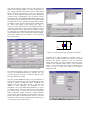
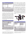
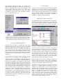
ATPDraw- Graphical Preprocessor to ATP. Windows version.
H. K. Høidalen
L. Prikler
J. L. Hall
SINTEF Energy Research
7034 Trondheim, NORWAY
[email protected]
SYSTRAN Engineering Services
Viola u. 7, H-2013 Pomáz, HUNGARY
[email protected]
Bonneville Power Administration
Portland, OR 97208-3621, USA
[email protected]
Abstract – ATPDraw is a graphical preprocessor to the
ATP-EMTP on the MS Windows platform. This paper
outlines some of the latest developments of ATPDraw,
including improved handling of MODELS, direct
execution of ATP, more components, and the User’s
Manual. The ongoing development is also presented.
Keywords: ATPDraw, ATP-EMTP, MODELS, graphical
pre-processor, Line/Cable Constants, modelling.
I. INTRODUCTION
ATPDraw is a graphical preprocessor to the ATP-EMTP
[1] on the MS Windows platform. In the program the user
can build up an electric circuit, using the mouse, by
selecting predefined components from an extensive palette.
Both single phase and 3-phase components are supported.
ATPDraw generates the ATP file in the appropriate format
based on "what you see is what you get". ATPDraw takes
care of the naming of unspecified nodes. All kinds of
standard circuit editing facilities (copy/paste, grouping,
rotate, export/import) are available. Most of ATP’s
standard components as well as TACS are supported, and
in addition the user can create new objects based on
MODELS [2] or Data Base Modularization. ATPDraw has
a standard Windows layout, supports multiple documents
and offers a large Windows help file system.
Along with ATPDraw comes a program called ATP_LCC
that supports Line/Cable Constants in the ATP-EMTP. In
this program the material and geometric data are specified
in dialog windows and the cross section is displayed in the
main window. ATP executions produce punch files that in
most cases are readable by ATPDraw. PI-circuits, KCLee
and JMarti formats are supported.
A. Improved handling of MODELS
Version 1.2 of ATPDraw for Windows is capable of
reading a mod-file directly, examine its input, output and
data variables, and creating an appropriate circuit objects
automatically. A mod-file is a text file in the MODELS [2]
language describing the actual model starting with MODEL
<ModelName> and ending with ENDMODEL. The mod-file
must be stored in <ModelName>.mod. Maximum 12
input+output variables are allowed along with 36 data
variables. As default, input nodes are basically positioned
on the left side of the icon and the outputs on the right.
Indexed variables are not allowed. Below, the header of a
mod-file is shown. When reading this file, ATPDraw
performs a message box shown in Fig. 1.
MODEL FLASH_1
INPUT V1
V2
iczn
DATA Pset
Eset
fdel
fdur
VAR power
trip
energy
tfire
vcap
OUTPUT trip
-------------
Voltage on positive side
Voltage on negative side
Current [Amps]
Power setting [MJ/ms]
energy setting [MJ]
firing delay [ms]
firing duration [ms]
power into ZnO [W]
gap firing signal[0 or 1]
energy into ZnO [J]
prev fire time [s]
voltage difference [V]
If the user clicks on Yes in Fig. 1, left, the edit support file
dialog box will appear where the user primarily can edit
the icon, change node positions and set new default values
for input type (current/voltage etc.). If the user selects No,
the default ATPDraw object is drawn in the circuit window
directly, as shown in Fig. 1, right.
The ATPDraw program is royalty free and can be
anonymously downloaded free of charge from the ftp
server ftp.ee.mtu.edu. ATPDraw has been continuously
developed since 1992. A User’s Manual that covers the
Windows version of ATPDraw is available [3]. The
functionality of ATPDraw is briefly listed in the appendix.
II. LATEST NEWS
This section lists some of the new facilities introduced in
ATPDraw since version 1.0 for Windows was launched in
June 1997. These are basically improved handling of
Models, direct execution of executable and batch files from
ATPDraw and new and improved components [4].
Fig. 1. Left: Read .mod file dialog box.
Right: Default model object (flash_1.sup).
Version 1.2 of ATPDraw also supports RECORD of model
variables. This option is found under ATP|Settings/Record
page as shown in Fig. 2.
In the list box under Model, all models in the active circuit
are listed. When selecting a model in this box its variables
are listed in the list box under Variable. When selecting a
variable here a default alias name appears in Alias. Edit
this name and click on Add to record the variable. The
Alias name can be changed by selecting an item in the
Record list box and type in a new name. The record list is
stored in the circuit file, but it does not follow the circuit
when using the clipboard or the export group option.
All the older circuit objects of version 1.0 are supported in
the new version, but some of them has been removed from
the Selection menu and replaced by other more general
components. The old objects can still be used in the circuit
and are found under User Specified|Files.. in the /SUP or
/TAC directories if absolutely required. They are supported
internally in ATPDraw and will produce the correct output.
Old circuit files will of course still contain these objects.
The objects added to ATPDraw in the new version are
listed in tab. 1.
Tab. 1. New components in ATPDraw.
Selection menu
Component file
Branch linear|
RLC3
RLC 3-ph
Fig. 2. Record of model variables.
B. Direct execution of ATP/TPPLOT
The user can specify programs to execute directly from
ATPDraw. The option is found under ATP|Edit batch jobs
as shown in Fig. 3, left. In this window the user can select
a name for the batch job (under Name), which file to
execute (under Launch file), and what kind of file to send
as parameter when calling this program (under Parameter).
Selecting Current ATP under Parameter will send the
name of the latest generated ATP file as parameter. When
selecting File, the user has to specify a file to send when
later launching the batch job. The specified batch jobs
appear in the main menu under ATP as shown in Fig. 3,
right. They are stored in the atpdraw.ini file.
Fig. 3. Left: The Edit batch job window
C. More components
Right: ATP menu.
Branch linear|
RLC-D 3-ph
RLCD3
Branch linear|
RLC-Y 3-ph
RLCY3
Branch nonlinear|
L(i) Type 96
NLIND96
Line distributed
Untransposed
LINEZU_2
Line distributed
Untransposed
LINEZU_3
Switches|
Statistic
SW_STAT
Switches|
Systematic
SW_SYST
Machines|
Universal|
synch, ind., 1-ph, DC
Transformers|
Saturable 3-phase
UM_1,
UM_3, UM_4,
UM_6, UM_8
GENTRAFO
TACS|
Transfer function
TRANSF
TACS|
Devices
DEVICE56
Line distributed|
Transp. lines (…
LINEZT_6
LINEZT6N
TYPE 94|
1 phase , 3 phase
TYPE94_1
TYPE94_3
Frequency comp.|
HFS Source
HFS_SOUR
Frequency comp.|
Cigre load 1/3 ph
CIGRE_1
CIGRE_3
Frequency comp.|
Linear RLC
RLC_F
Icon
Several generalised components have been introduced. A
new TACS laplacian transfer function with optional and
flexible limit settings replaces six older components. A
new 3-phase saturable transformer model is added which
allow 3 windings and selection of type of coupling and
reluctance. The component dialog box of this transformer
is shown in Fig. 4. Checking the 3-leg core button, turn the
transformer into a TRANSFORMER THREE PHASE type
with high homopolar reluctance, which is specified instead
of magnetisation losses. Checking the RMS button, enables
specification of the saturation characteristic in RMS values
for current and voltage on the Characteristic page. A
conversion to flux-current values is performed internally in
ATPDraw. If the button is not checked normal flux-current
values should be entered. Three type of winding couplings
are supported; Wye, Delta lead, and Delta lag (more types
will be added later). Icons visualise the selected coupling.
The tertiary winding can be turned on or of by checking
the 3-wind. button.
Fig. 5. Type 94 component dialog box.
A
B
t=0
1 mH
Figure 6. Type 94 component and steady-state specifications.
Fig. 4. General 3-phase transformer component dialog.
ATPDraw now supports Harmonic Frequency Scan, as
shown in Fig. 7. Under Simulation type the user can switch
between time domain, frequency scan, and harmonic
(HFS). The various new output formats from ATP is also
supported and selectable under Output. A new harmonic
source is also introduced with a component dialog box as
shown in Fig. 8, along with some new frequency
dependent loads.
New statistic/systematic switches are introduced with the
concept of independent/master/slave included. The user
can select the type of switch in a combo box and the rest of
the object adapts this setting.
The new Type94 MODELS objects [2,5] are handled in a
special way. When selecting a type 94 component the user
first has to specify a model file (*.mod). ATPDraw then
diagnoses this file like shown in Fig. 1 and finds the
number of data parameter and establishes a new
component. The two standard data parameters (n, ng/n2)
are always ignored. The user can in the components dialog
box, shown in Fig. 5, specify the type of 94 component
THEV (Thevenin), NORT (Norton) or ITER (Iterated),
along with the data paramer(s) and node names. The user
also has the option to add steady-state values to a type 94
component. This is done be specifying node names e.g. by
constructing a circuit shown in Fig. 6.
Fig. 7. Selecting type of simulation.
manual is divided in six parts. Parts 1-3 introduce
ATPDraw and explain how to get started with the program.
Part 4 is a reference manual listing all menus and
components (except for the new one listed in part II of this
paper). Part 5 is an advanced manual with several
illustrative and useful examples. Part 6 covers the line and
cable modelling supported by the auxiliary program
ATP_LCC for ATP’s LINE- and CABLE-CONSTANTS.
Fig. 8. Harmonic source component dialog box.
The handling of electrical machines has been updated
substantially. Several universal machines are allowed with
global specification of initialisation method and interface.
Synchronous machine (type 1), two types of induction
machines (type 3 & 4), DC machine (type 8) and a singlephase machine (type 6) are supported. The universal
machine component dialog box is shown in Fig. 9. The
user enters the machine data in five pages. On the first
some general data like stator coupling and the number of d
and q axis coils are specified. The Global data are set
under the UM page in Fig. 7. On the Magnet. page the
flux/inductance data with saturation are specified. On the
Stator and Rotor pages the coil data are given, and under
Init the initial conditions.
The advanced manual explains how to use MODELS and
User Specified Objects (USP) in ATPDraw. USPs are
external modules written in correspondence with ATP’s
DATA BASE MODULARIZATION technique, and
represented in ATPDraw with basically an icon and a
pointer to the external file. Node names and data values
can be sent as parameters when calling this external
module from ATP. Chapter 5.4 in the advanced manual
shows an example of how to model a 6-pulse thyristor
bridge as a USP and how to use this component to
construct a simple HVDC station, as shown in Fig. 10. Fig.
11 shows the USP’s component dialog where the
thyristor’s fire angle and the snubber circuit can be
specified.
U
POS1
VINV
VS
U
POS2
Fig. 10. 12-pulse rectifying station.
Fig . 9. Synchronous machine type 3 component dialog.
III. USER’S MANUAL
Fig. 11. Component dialog of 6-pulse thyristor bridge.
A User’s Manual for ATPDraw version 1.0 for Windows is
available [3]. This is a 193-page manuscript is also
available as an electronic document in pdf format via ftp at
ftp.ee.mtu.edu/pub/atp/atpdraw/Manual/atpwpdf.zip. The
The difficult part of the USO construction is the
development of the Data Base Module file, but this task is
only performed once for each object.
The advanced manual also shows an example of a
lightning study using JMarti overhead lines, a ground fault
study, a transformer inrush study using BCTRAN with
external added saturation elements etc. When using
overhead lines circuits ATPDraw is in many cases capable
of reading the punch files from Line/Cable Constants
directly as illustrated in Fig. 12.
V. CONCLUSION
ATPDraw is continuously developed and the new facilities
added since June 1997 are mainly: improved handling of
MODELS, direct execution of external programs like ATP,
new and more powerful components, and a User’s Manual.
On the schedule are further improvements in handling of
MODELS and inclusion of Line/Cable modelling in
ATPDraw by support of Cable Parameters.
APPENDIX ATPDraw functionality.
The appendix lists some of the functionality in ATPDraw.
Much more information is found in the User’s Manual [3].
Fig. 13 shows the main window in ATPDraw, with some
open circuit windows and the Selection menu to the right.
Fig. 12. Process of generating a 3-phase overhead line from a
punch file. Top left: Selecting an overhead line punch file. Right:
ATPDraw diagnosis, lib-file on Data Base Module format autocreated. Bottom left: Default component icon for use in circuit.
IV. FUTURE DEVELOPMENTS
ATPDraw does not support or facilitate the usage of the
MODELS language. The user must write his own model
file without the assistance from ATPDraw. The plan is to
extend the present text editor in ATPDraw and add some
tools to assist the user when writing a model file. This will
include some help files and automatic inclusion of the
model’s structure. The editor will also make sure that the
model file is stored in the correct directory with the correct
extension.
The new separate Line/Cable Constant supporting program
ATP_LCC is on a prototype level. The schedule is to
include and improve the facilities of ATP_LCC directly in
ATPDraw and to support CABLE PARAMETERS only.
Selecting a line model in the component selection menu
will bring up a dialog box where the cross section of a line
or cable can be specified with its geometry and material
data. Execution of ATP will be performed automatically to
create a punch file from Cable Parameters. This file will
next be filtered with an already built in module in
ATPDraw to create a Data Base Module file that could be
included in a circuit. The whole process with files and
ATP executions will be hidden from the user who only
sees the cross section and the final ATPDraw component.
A possible next step would be to also support the Line
Model Frequency Scan for verification of the correctness
of the line/cable model.
Fig. 13. ATPDraw main window.
From the Selection menu the user selects components to
insert into the circuit. This menu pops up when clicking the
right mouse button in an empty area of a circuit window.
To select and move an object, simply press and hold down
the left mouse button on the object while moving the
mouse. Release the button and click in an empty area to
unselect and confirm the new position. The object is then
moved to the nearest grid point (10 pixels resolution).
Overlapping components will produce a warning.
Selected objects or a group can be rotated by clicking on it
with the right mouse button. Other object manipulation
functions, such as undo/redo and clipboard options can be
found in the Edit menu as well as on the tool bar.
Selection of a group of objects for moving can be done in
three ways: 1) Holding down the Shift key while leftclicking on an object adds it to the current group. 2)
Holding down the left mouse button in an empty area and
drag will draw a rectangular outline around the desired
objects. 3) Double-clicking the left mouse button in an
empty area enables the creation of a polygon shaped
region. Corners are created with left button clicks and the
region is enclosed with a right click. Objects within the
drawn region become a group. An object and a group of
objects are moved and edited the same way.
It is possible to draw much larger circuits than shown on
the screen in normal zoom mode. The circuit world is
5000x5000 pixels. The user can move around in this world
using the window scrollbars or by dragging the view
rectangle in the Map Window. The Map Window (shortcut
key: M) gives a view of the whole circuit world and a
rectangle showing the current circuit window position.
Selected objects do not follow the scrollbars or the map
window but stay fixed on the screen. Thus, usage of the
e.g. scrollbars will move a selected group in the circuit
world.
Components and component nodes can be opened for
editing. If the user right-click or left double-click on an
unselected component or node, either the Component or
the Node dialog box will appear where component or node
attributes and characteristics can be edited. Click on the
Help button to get component specific help, and press F1
to get general help on the dialog box. Default component
attributes are stored in support files. Access to create and
customise support files is provided under Objects in the
main menu. Node names should normally be specified in
the Node dialog box, and only nodes of special interest
need to be named. ATPDraw handles the whole node
naming process.
Components are connected if their nodes overlap or if a
connection is drawn between the nodes. To draw a
connection between nodes, click on a node with the left
mouse button. A line is drawn between that node and the
mouse cursor. Click the left mouse button again to place
the connection (clicking the right button cancels the
operation). The gridsnap facility helps overlapping the
nodes. Connected nodes are given the same name by the
Make Names and Make File options in the ATP menu.
Nodes can be attached along a connection as well as at
connection end-points. A connection should not
unintentionally cross other nodes (what you see is what
you get). A warning for node naming appears during the
ATP file creation if a connection exists between nodes of
different names, or if the same name has been given to
unconnected nodes. Connections can be selected as any
other objects. To resize a connection, click on its end-point
with the left mouse button, hold down and drag. If several
connections share the same node, the desired connection to
resize must be selected first. Selected connection nodes are
marked with squares at both ends of the selection
rectangle. Connections from a 3-phase node are visualised
as thick.
Tab. 2 Mouse operations in ATPDraw.
Mouse
Unselected
button
Component
Left simple Select
- component
- connection
Right simple Open
comp. dialog
Mouse click on/in
Selected
Node
Component
Draw
connection
Rotate
-.component
- connection
- group
Left hold
Move
Move
component - component
- group
Left double Open
Open group
comp. dialog dialog
Open
space
Unselect +
Place
connection
Open
Selection
node dialog menu +
Cancel
connection
Resize
Select
connection group
Rectangle
Open
Select
node dialog group
Polygon
ATPDraw offers the most common edit operations like
copy, paste, duplicate, rotate and delete. The edit options
operate on a single object or on a group of objects. Objects
must be selected before any edit operations can be
performed. Selected objects can also be exported to a disk
file and any circuit files can be imported into another
circuit.
The circuit drawing can be stored on a specially formatted
binary file called cir-file, by selecting Save or Save As
under File in the main menu. ATPDraw can read cir-files
from all Windows versions, but a separate program called
CONVERT is required to retrieve files from the DOS
version 3. A program called cir2-3.exe converts cirfiles between DOS versions 2 and 3.
The ATP menu shown in Fig. 3, right, includes selections
for setting the miscellaneous ATP cards, creating an ATP
file, study the created ATP file and the printed output of a
simulation, making node names (also called automatically
when selecting Make file), and finally specifying files to
execute from ATPDraw.
ACKNOWLEDGEMENT
The work on ATPDraw is possible due to financing from
U.S. Dept. of Energy, Bonneville Power Administration
and Pacific Engineering Corporation.
REFERENCES
Three phase nodes are given the extensions A/B/C (or
D/E/F) automatically by ATPDraw. Rotation of the phase
sequence is possible by usage of special transposition
objects. A special Splitter object handles connections
between 3-phase and single-phase sub-circuits. These
special objects are found under the Probes&3-phase field
in the Selection menu.
Tab. 2 contains a summary of the various actions taken
dependent on mouse operations. The left mouse button is
generally used for selecting objects or connecting nodes;
the right mouse button is used for specification of object or
node properties.
[1]
[2]
[3]
[4]
[5]
Alternative Transients Program (ATP) - Rule Book,
Canadian/American EMTP User Group, 1987-1998.
L. Dubé, ”Models in ATP”, Language manual, Feb.
1996.
L. Prikler, H.K. Høidalen, ATPDraw User’s Manual,
SEfAS TR A4790, ISBN 82-594-1358-2, Oct. 1998.
H.K. Høidalen, “ATPDraw for Windows, Version 2”.
Proceedings of the 1998 European EMTP Users Group
Meeting, Nov. 8-10, Prague.
L. Dubé, “How to use MODELS-based user-defined
network components in ATP”. Proceedings of the 1996
European EMTP Users Group Meeting, Nov. 10-12,
Budapest.