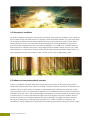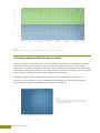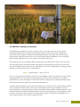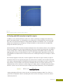
1
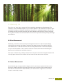
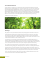
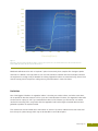
LA I THEORY & PRACTICE We measure the world. Leaf Area Index ( LAI ) is one of the most widely used measurements for describing plant canopy structure. LAI is also useful for understanding canopy function because many of the biosphere-atmosphere exchanges of mass and energy occur at the leaf surface. For these reasons, LAI is often a key biophysical variable used in biogeochemical, hydrological, and ecological models. LAI is also commonly used as a measure of crop and forest growth and productivity at spatial scales ranging from the plot to the globe. In the past, measuring LAI was difficult and time consuming. However, theory and technology developed in recent years have made measuring LAI much simpler and more feasible for a wide range of canopies. The following information is intended to provide a brief introduction to the theory and instruments used to measure LAI. Several scenarios and special considerations are covered, which will help individuals choose and apply the most appropriate method for their research needs. LAI: Theory and Practice v. I.0 Copyright©2014. Decagon Devices, Inc. All Rights Reserved. Printed in the U.S.A Table of Contents 1. What is LAI?………………………………………………………………………… I 2. How to Measure LAI……………………………………………………………… 2 2.1. Direct measurement……………………………………………………………… 2 2.2. Indirect measurement…………………………………………………………… 2 2.2.1. Hemispherical photography…………………………………………………… 2 2.2.2. Radiation transmittance……………………………………………………… 3 2.2.3. Radiation reflectance………………………………………………………… 4 3. Using the LP-80 Ceptometer……………………………………………………… 7 3.1. Short canopies…………………………………………………………………… 9 3.2. Tall canopies……………………………………………………………………… 9 3.3. Clumping and spatial sampling………………………………………………… I0 3.4. Atmospheric conditions………………………………………………………… II 3.5. Influence of non-photosynthetic elements…………………………………… II 4. Using the SRS-NDVI Sensor……………………………………………………… I2 4.1. Developing field-based NDVI-LAI regression models………………………… I3 4.2. SRS-NDVI sampling considerations…………………………………………… I4 4.3. Influence of soil background on NDVI measurements……………………… I5 4.4. Dealing with NDVI saturation in high LAI canopies…………………………… I6 References…………………………………………………………………………… I8 I. What is LAI? Leaf Area Index ( LAI ) quantifies the amount of leaf material in a canopy. By definition, it is the ratio of onesided leaf area per unit ground area. LAI is unitless because it is a ratio of areas. For example, a canopy with an LAI of 1 has a 1:1 ratio of leaf area to ground area (Fig. 1a). A canopy with an LAI of 3 would have a 3:1 ratio of leaf area to ground area (Fig. 1b). Globally, LAI is highly variable. Some desert ecosystems have an LAI of less than 1, while the densest tropical forests can have an LAI as high as 9. Mid-latitude forests and shrublands typically have LAI values between 3 and 6. Seasonally, annual and deciduous canopies and croplands can exhibit large variations in LAI. For example, from seeding to maturity, maize LAI can range from 0 to 6. Obviously, LAI is a useful metric for describing both spatial and temporal patterns of canopy growth and productivity. a Ground Area = 1 m2 Leaf Area = 1 m2 LAI=Leaf Area: Ground Area = 1:1 = 1 b Ground Area = 1 m2 Leaf Area = 3 m2 LAI=Leaf Area: Ground Area = 3:1 = 3 Figure I. Conceptual diagram of a plant canopy where (a) LAI = 1 or (b) LAI = 3. I Defining LAI 2. Measuring LAI There is no one “best” way to measure LAI. Each method has advantages and disadvantages. The method you choose will depend largely on your research objectives. The researcher who needs a single estimate of LAI might use a different method than the one who is monitoring changes in LAI over time, for example, and the grassland researcher may prefer a different method than the forestry researcher. In this guide, we’ll discuss the theoretical basis of each of the major methods along with key advantages and limitations. 2.1 Direct Measurement Traditionally, researchers measured LAI by harvesting all the leaves from a plot and painstakingly measuring the area of each leaf. Modern equipment like flatbed scanners have made this process more efficient, but it is still labor intensive, time consuming and destructive. In tall forest canopies, it may not even be feasible. It does, however, remain the most accurate method of calculating LAI because each individual leaf is physically measured. Litter traps are another way to directly measure LAI, but they don’t work well in evergreen canopies and can only capture information from leaves that have senesced and abscised from the plant. 2.2 Indirect Measurement Several decades ago, canopy researchers began to look for new ways to measure LAI, both to save time and to avoid destroying the ecosystems they were trying to measure. These indirect methods infer LAI from measurements of related variables, such as the amount of light that is transmitted through or reflected by a canopy. Measuring LAI 2 Figure 2. Hemispherical photograph acquired from a mixed deciduous forest using a digital camera fisheye lens. 2.2.I Hemispherical Photography Hemisphere photography was one of the first methods used to indirectly estimate LAI. Researchers would photograph the canopy from the ground using a fisheye lens (Fig. 2). Photographs were originally analyzed by researchers themselves. Now, most researchers use specialized software to analyze images and differentiate between vegetated and non-vegetated pixels. Advantages Hemispherical photography has decided advantages. First, it delivers more than just LAI measurements. It can also provide canopy measurements such as gap fraction, sunfleck timing and duration, and other canopy architecture metrics. Second, the canopy images can be archived for later use or for reanalysis as methods change and software programs improve. Limitations Hemispherical photography has drawbacks, however. In spite of the fact that the images are now digitally processed, user subjectivity remains a significant issue. Users must select image brightness thresholds that distinguish sky pixels from vegetation pixels, causing LAI values to vary from user to user or when using different image analysis algorithms. Hemispherical photography also remains time consuming. It takes time to acquire good quality images in the field and more time to analyze the images in the lab. Also, sky conditions must be uniformly overcast when the pictures are taken. Hemispherical photography does not work well for short canopies like wheat and corn since the camera body, lens, and tripod may not physically fit under the canopy. For some users, instruments that measure PAR offer a shortcut. Some models use LAI values to estimate PAR. In this case, the PAR instrument can be used to directly estimate below-canopy levels of PAR, improving the accuracy of the model. 3 Measuring LAI 2.2.2 Radiation Transmittance Several commercially available instruments, including Decagon’s LP-80 ceptometer, offer an alternative to hemispherical photography. They estimate LAI using the amount of light energy transmitted by a plant canopy. The idea is fairly simple: a very dense canopy will absorb more light than a sparse canopy. This means there must be some relationship between LAI and light interception. Beer’s law provides the theoretical basis for this relationship. For the purposes of environmental biophysics, Beer’s law is formulated as: Equation I PARt = PARi exp ( – kz ) where PARt is transmitted photosynthetically active radiation (PAR) measured near the ground surface, PARi is PAR that is incident at the top of the canopy, z is the path length of photons through some attenuating medium, and k is the extinction coefficient. In the case of vegetation canopies, z accounts for LAI, since leaves are the medium through which photons are attenuated. You can see that if we know k and measure PARt and PARi it may be possible to invert Eq. 1 to calculate z as an estimate of LAI. This approach is commonly referred to as the PAR inversion technique. The real world is slightly more complex, but as you will see in Section 3, Beer’s law is the foundation for estimating LAI using measurements of incident and transmitted PAR. Advantages The PAR inversion technique is non-destructive, one obvious but major advantage that allows a canopy to be sampled extensively and repeatedly through time. The PAR inversion technique is also attractive because it has a solid foundation in radiative transfer theory and biophysics and is applicable in a wide variety of canopy types. For these reasons, the PAR-inversion technique is currently a standard and wellaccepted procedure. In addition to handheld instruments like Decagon’s LP-80 ceptometer, standard PAR sensors (a.k.a. quantum sensors) can also be used to measure transmitted radiation for a PAR-inversion model. The advantage to using PAR sensors as opposed to a purpose-built, handheld LAI instrument is that PAR sensors can be left in the field to continuously measure changes in PAR transmittance. This may be useful when studying rapid changes in canopy LAI or when it is not feasible to visit a field site frequently enough to capture temporal variability in LAI with a handheld instrument. Limitations The PAR inversion technique has a few limitations. It requires measurements of both transmitted (below canopy) and incident (above canopy) PAR under identical or very similar light conditions. This can be challenging in very tall forest canopies, although incident PAR measurements can be made in large canopy gaps or clearings. Also, in extremely dense canopies PAR absorption may be nearly complete, leaving little transmitted light to be measured at the bottom of a canopy. This makes it difficult to distinguish changes or differences in LAI when LAI is very high. Finally, estimates of LAI obtained from measurements of transmitted PAR can be affected by foliage clumping. Errors in LAI estimation associated with clumping can usually be alleviated by collecting numerous spatially distributed samples of transmitted PAR. Measuring LAI 4 2.2.3 Radiation Reflectance Another method for estimating LAI uses reflected rather than transmitted light. Radiation that has been reflected from green, healthy vegetation has a very distinct spectrum (Fig. 3). In fact, some scientists have proposed finding potentially habitable planets outside our solar system by looking for this unique spectral signal. A typical vegetation reflectance spectrum has very low reflectance in the visible portion of the electromagnetic spectrum (~400-700 nm, which is also the PAR region). However, in the near-infrared (NIR) region (> 700 nm) reflectance can be as high as 50%. The exact amount of reflectance at each wavelength depends on the concentration of various foliar pigments like chlorophyll and canopy structure (e.g., arrangement and number of leaf layers). Advantages Early attempts to use spectral reflectance data to quantify canopy properties found that the ratio of red and NIR reflectance could be used to estimate the percent canopy cover for a given area. Later efforts have produced a number of different wavelength combinations that relate to various canopy properties. These wavelength combinations, or spectral vegetation indices, are now routinely used as proxies for LAI or, through empirical modeling, are used to directly estimate LAI. Until recently one of the only ways to collect reflectance data was with a handheld spectrometer—an expensive, delicate instrument designed for the lab, not the field. But sensor options have expanded with the development of lightweight multiband radiometers that measure a specific vegetation index. These little sensors are inexpensive and don’t require a lot of power, making them perfect for field monitoring. This is good news for anyone who wants to monitor changes in LAI over time, including researchers interested in phenology, canopy growth, detecting canopy stress and decline, or detecting diseased plants. Vegetation indices offer another advantage: many earth-observing satellites like Quickbird, Landsat, and MODIS measure reflectance that can be used to calculate vegetation indices. Since these satellites observe large areas, they may serve as a way of scaling observations made at the local scale to much broader areas. Conversely, measurements made at the local scale with a multiband radiometer can be a useful source of ground truth data for satellite-derived vegetation indices. 5 Measuring LAI 0.05 0.45 0.4 Reflectance 0.35 0.03 0.25 0.2 0.15 0.I 0.05 0 400 500 600 700 800 900 I,000 Wavelength(nm) Figure 3. Reflectance Spectra obtained at different stages of canopy development. Note the distinct difference between visible and near infrared (NIR) reflectance that develops as LAI increases. Multiband radiometers also offer a “top down” option for extremely short canopies like shortgrass prairie and forbs. It’s difficult if not impossible to use most LAI estimation methods with these canopies, because the equipment is too big to fully fit beneath the canopy. Vegetation indices are measured using sensors that view the canopy from the top down, making them a great alternative in cases like these. Limitations One of the biggest limitations of vegetation indices is that they are unitless values, and when used alone, do not provide an absolute measure of LAI. If you don’t need absolute LAI values, the vegetation index value can be used as a proxy for LAI. If you need absolute values of LAI, however, you will need to use another method for measuring LAI in conjunction with the vegetation index until enough co-located data has been gathered to produce an empirical model. This method can also be limited due to the location of sensors. By nature, reflectance must be measured from the top of a plant canopy, which may not be feasible in some tall canopies. Measuring LAI 6 3. Using the LP-80 ceptometer Decagon’s LP-80 ceptometer uses the PAR inversion technique for calculating LAI. The LP-80 uses a modified version of the canopy light transmission and scattering model developed by Norman and Jarvis (1975). Five key variables used as inputs are discussed below. τ (ratio of transmitted and incident PAR): The most influential factor for determining LAI with any PAR inversion model is the ratio of transmitted to incident PAR. This ratio (τ) is calculated using measurements of transmitted PAR near the ground surface and incident PAR above the canopy. 86.5 cm τ is a relatively intuitive variable to understand. When LAI is low, most incident radiation is transmitted through the canopy rather than being absorbed or reflected it, thus τ will be close to 1. As the amount of leaf material in the canopy increases, there is a proportional increase in the amount of light absorbed and a decreasing proportion of light will be transmitted to the ground surface. The LP-80 consists of a light bar, which has 80 linearly spaced PAR sensors, and an external PAR sensor. In typical scenarios, the light bar is used to measure PAR under the canopy, whereas the external sensor is meant to quantify incident PAR, either above the canopy or in a clearing. Additional measurement scenarios are covered in Sections 3.1 and 3.2. θ (solar zenith angle): θ is the angular elevation of the sun in the sky with respect to the zenith, or the point directly over your head, at any given time, date, and geographical location (Fig.4). The solar zenith angle is used to describe the path length of photons through the canopy (e.g., in a closed canopy the path length increases as the sun approaches the horizon), and for determining the interaction between beam radiation and leaf orientation (discussed below). θ is automatically calculated by the LP-80 using inputs of local time, date, latitude and longitude. Therefore, it is critical to make sure that these are correctly set in the LP-80 configuration menu. ƒb (beam fraction): In an outdoor environment, the ultimate source of shortwave radiation is the sun. When the sky is clear, most radiation comes as a beam directly from the sun (Fig. 5a). In the presence of clouds or haze, however, some portion of the beam radiation is scattered by water vapor and aerosols in the atmosphere (Fig. 5b). This scattered component is referred to as diffuse radiation. ƒb is calculated as the ratio between diffuse and beam radiation. The LP-80 automatically calculates fb by comparing measured values of incident PAR to the solar constant, which is a known value of light energy from the sun (assuming clear sky conditions) at any given time and place on earth’s surface. χ (leaf angle distribution): The leaf angle distribution parameter (χ) describes the projection of leaf area onto a surface. Imagine, for example, a light source directly overhead. The shadow cast by a leaf with a vertical orientation would be much smaller than the shadow cast by a leaf with a horizontal orientation. In nature, canopies are typically composed of leaves with a mixture of orientations. This mixture is often best described by what is known as the spherical leaf distribution with a χ value = 1 (the default in the LP-80). Canopies with predominately horizontal orientations, such as strawberries, have χ values > 1, whereas canopies with predominately vertical orientations, like some grasses, have χ values < 1. Extensive details about the LP-80’s LAI model are provided in the user’s manual: www.decagon.com/education/lp-80-manual/ 7 Using the LP-80 Ceptometer a b Figure 4. Solar zenith angle changes during the day. Observer is facing the equator (Left). Figure 5. Beam fraction under (a) sunny and (b) overcast sky conditions (Right). In general χ describes how much light will be absorbed by the leaves in a canopy at different times of day as the sun moves across the sky. The estimation of LAI with the PAR inversion technique is not overly sensitive to the χ value, especially when sampling under uniformly diffuse sky conditions (Garrigues et al., 2008). The χ value is most important when working with canopies displaying extremely vertical or horizontal characteristics and when working under clear sky conditions where fb is less than approximately 0.4. For additional information about leaf angle distribution, the reader is referred to Campbell and Norman (1998). K (extinction coefficient): The canopy extinction coefficient, K, describes how much radiation is absorbed by the canopy at a given solar zenith angle and canopy leaf angle distribution. The concept of an extinction coefficient comes from Beer’s law (Eq. 1). A detailed explanation of the extinction coefficient can quickly become complicated. For LAI estimation it is sufficient to know that the angle of solar beam penetration interacts with leaf angle distribution to determine the probability that a photon will be intercepted by a leaf. For purposes of estimating LAI, K is calculated as: Equation 2 K= √ χ2+tanθ 2 χ+1.744 (χ+1.182)-0.733 From this equation it should be obvious that, for any given canopy, K only changes as the sun moves across the sky. The LP-80 automatically calculates K each time it measures LAI. Once K is calculated and all other variables quantified, LAI is calculated as: Equation 3 L= [(1- 2K1 ) ƒb-1 )] 1n τ A(1-.047ƒb) where L is LAI and A is leaf absorptivity. By default A is set to 0.9 in the LP-80. Leaf absorptivity is a highly consistent property for most healthy green foliage and a value of 0.9 is a good approximation for most situations. In extreme cases (e.g., extremely young leaves, highly pubescent or waxy leaves, senescent leaves) A may deviate from 0.9, leading to errors in estimates of LAI. If you are using the LP-80 in nontypical conditions you may need to manually combine the outputs from the LP-80 with a modified A value to calculate LAI. Using the LP-80 Ceptometer 8 3.I Using the LP-80 in short canopies (e.g., cereal crops, grasslands) In typical scenarios it is best to hold the ceptometer at a consistent height underneath the canopy, while the attached external PAR sensor is held above the canopy. Use the attached bubble level to ensure that the light bar and external PAR sensor are held level. For row crops or small sample plots, researchers often mount the external sensor on a tripod in between rows or above the canopy. The LP-80 makes simultaneous above- and below-canopy PAR measurements each time the button is pressed, accounting for any changes in light conditions. If the canopy is short enough, an even easier approach is to use the ceptometer to acquire both above and below canopy measurements. Simply hold the LP-80 above the canopy to acquire an incident PAR measurement. Update the above canopy measurement every few minutes or as sky conditions change (e.g., due to variable clouds). In either case, all the other variables discussed in Section 3 are measured and calculated automatically, and LAI is updated with each below canopy measurement. 3.2 Using the LP-80 in tall canopies (e.g., forests, riparian areas) In tall canopies it is often not practical to measure above and below-canopy PAR with one instrument. When using the LP-80 in tall canopies there are a couple of options available for making above and below canopy measurements of PAR. One option is to mount a PAR sensor above the canopy or in a wide clearing with an unobstructed view of the sky. This method requires some additional post-processing of the data, but can give good results. The PAR sensor needs to be attached to its own data logger, which should be configured to acquire measurements at regular intervals (e.g., every 1-5 minutes) so that any variation in ambient light levels will be captured. You should collect below canopy measurements with the ceptometer as you normally would, then combine the data in post processing, using the timestamps to pair each above- and below-canopy measurement. Calculate τ with each pair, which can then be used as an input to Equation 3. 9 Using the LP-80 Ceptometer The second option is useful to use when it is not feasible to place a PAR sensor above the canopy or when a PAR sensor or data logger is not available. If this is the case then you can use the LP-80 to measure incident PAR in a location outside the canopy with an unobstructed view of the sky. In measurement mode, you can choose whether you are measuring incident or transmitted radiation. When using the LP-80 itself to take above and below canopy readings, you should take the variability of sky conditions into account. On a clear sky day, it is easiest to acquire samples toward the middle of the day, since the light levels won’t change much over the span of 20 to 30 minutes. When sky conditions are uniformly overcast, PAR conditions can remain sEquation 6 for longer periods of time, giving you a longer measurement window before needing to reacquire an above canopy measurement. If sky conditions are highly variable, however, we do not recommend this method unless you can constantly update the incident PAR measurement. The LP-80 automatically calculates LAI with each below-canopy measurement using the stored incident PAR measurement. Reacquire an incident PAR measurement any time light conditions change (e.g., when cloud obstructs the solar disk, or after ~ 20-30 minutes have passed) to prevent error in the LAI calculation. 3.3 Clumping and spatial sampling In most canopies, LAI is variable across space. For example, in row crops, LAI can range from 0 to 2-3 within a distance of 1 meter. Even in forests and other natural canopies, variable tree spacing, branching characteristics, and leaf arrangement on stems causes clumping. This means that pointbased measurements of LAI can be highly biased. Lang and Yueqin (1986) found that averaging several measurements along a horizontal transect helped alleviate biases associated with clumping at fine spatial scales. The LP-80 uses a similar approach, averaging light measurements across eight groups of ten sensors situated along an 80 cm long probe. Although this approach reduces errors at the local scale, it may not account for variability in LAI at the canopy scale. Researchers must consider spatial variability in canopy LAI when developing a sampling scheme. In general, more heterogeneous canopies will require more LAI measurements across space in order to obtain a LAI value that is representative of the entire canopy. Using the LP-80 Ceptometer 10 3.4 Atmospheric conditions The LP-80 is capable of accurately measuring LAI in both clear sky and overcast conditions. This is because the LAI model used by the LP-80 accounts for changes in diffuse and beam radiation (ƒb), solar zenith angle (θ ), and because incident and transmitted radiation are measured simultaneously when using an abovecanopy PAR sensor. Errors associated with incorrectly specifying the leaf angle distribution (χ) are most pronounced when sampling under clear sky conditions (Garrigues et al., 2008). This is because there is a larger proportion of radiation coming from a single angle (the beam radiation directly from the sun). Under these conditions it is important to correctly model how leaf angle and beam penetration angle interact. So, when sampling under clear sky conditions make sure that you are using an appropriate χ value. 3.5 Influence of non-photosynthetic elements In forests, shrublands, and other areas where woody species are present, LP-80 measurements will be influenced by elements other than leaves. For example, tree boles, branches, and stems will intercept some radiation, and thus have an effect on estimates of LAI obtained with the PAR inversion technique. In fact, some researchers refer to the measurement obtained from the LP-80 and similar instruments to Plant Area Index (PAI) rather than LAI, in order to acknowledge the contribution of non-leaf material to the measurement. It should come as no surprise that PAI will be higher than LAI in any given ecosystem. However, values of PAI and LAI are often not too different because leaf area is generally much larger than branch area and the majority of branches are shaded by leaves (Kucharik et al., 1998). In deciduous ecosystems, the contribution of woody material can be accounted for by acquiring measurements during the “leaf-off” stage. II Using the SRS-NDVI Sensor In depth technical SRS-NDVI specifications and operating details are provided in the manual, which can be accessed on the web decagon.com/support/manual-spectral-reflectance-sensor-srs/ 4. Using the SRS-NDVI sensor The SRS-NDVI sensor measures canopy reflectance in red and NIR wavelengths, which allows for calculation of the Normalized Difference Vegetation Index (NDVI). In turn, NDVI can be used to estimate LAI. We provide a brief overview of the SRS-NDVI operating theory here. The SRS-NDVI measures canopy reflectance in red and NIR wavelengths, and its measurements can be used to calculate or approximate LAI. Red and NIR reflectances are used the following equation to calculated NDVI: Equation 4 where ρ denotes percent reflectance in NIR and red wavelengths. Mathematically, NDVI can range from -1 to 1. As LAI increases, red reflectance will typically decrease due to increasing canopy chlorophyll content, whereas NIR reflectance increases due to expanding mesophyll cells and increasing canopy structural complexity. So, under typical field conditions NDVI values typically range from somewhere around 0 to 1, representing low and high LAIs, respectively. In cases like phenology and “stay green” phenotyping where absolute values of LAI are not required, NDVI values can be used directly as proxies for LAI. For example, if the objective of a study is to track the temporal patterns of canopy growth and senescence (Fig. 6), then it may be adequate to simply use NDVI as the metric. If your research objectives require estimates of actual LAI, it is possible to establish a canopyspecific model that will allow NDVI to be converted to LAI. This method is described in the next section. Using the SRS-NDVI Sensor I2 Leaf Area Index 4 3 2 NDVI 0.8 0.6 0.4 2000 2001 2002 2003 2004 2005 2006 2007 Year Figure 6. NDVI closely tracks the year-to-year seasonal dynamics of LAI in a mixed deciduous forest. 4.I Developing field-based NDVI-LAI regression models To directly estimate LAI using NDVI values, you need to develop a site-specific or crop-specific correlative relationship. The best way is to take co-located measurements of NDVI and LAI (e.g., using a LP-80 ceptometer). For example, co-located measurements of LAI and NDVI were acquired during a period of rapid canopy growth. Least squares regression was used to fit a linear model to the data (Fig. 7). With this model, we can use NDVI to predict LAI without making independent measurements. Developing a robust empirical model involves some effort, but once the model is complete, you can continuously monitor changes in LAI with a SRS-NDVI sensor deployed over a plot or canopy long term. This method can ultimately save significant effort and time in the long run. 3.5 3 LAI 2.5 Figure 7. Relationship between NDVI and LAI. The fitted linear regression model (solid line) can be used to predict LAI from NDVI measurements. 2 I.5 I 0.5 0 0.3 0.4 0.5 0.6 NDVI I3 Using the SRS-NDVI Sensor 0.7 0.8 0.9 4.2 SRS-NDVI sampling considerations The SRS-NDVI is designed to be used as a dual view sensor. This means that one sensor, having a hemispherical field of view, should be mounted facing toward the sky. The other sensor, having a 36° field of view (18° half angle), should be mounted facing downward at the canopy. Down and up looking measurements collected from each sensor are used to calculate percent reflectance in the red and NIR bands. Percent reflectances are used as inputs to the NDVI equation (Eq. 4). The up looking sensor must be placed above any obstructions that will block the sensor’s view of the sky. The down looking sensor should be directed at the region of the canopy to be measured. The size of the area measured by the down looking sensor is dependent on the sensor’s height above the canopy. The spot diameter of the down looking sensor is calculated as: Equation 5 Spot Diameter = (tan (γ) x h)2 x π where γ is the half angle of the field of view (18° for the SRS-NDVI), and h is the height of the sensor above the canopy. Equation 5 is valid for measuring spot diameter when the down looking sensor is pointed straight down (i.e., nadir view angle). In cases where the down looking sensor is pointing off-nadir, the spot will be oblique and will be larger than that calculated by Equation 5. To quantify spatial variability in LAI, several down looking sensors can be set up to monitor different portions of the canopy. For example, several sensors were mounted above the canopy in a deciduous forest to monitor differences in spring phenology of several trees. Measurements of NDVI revealed differences in the timing and magnitude of leaf growth among the trees that were measured (Fig. 8). A similar approach could be used to monitor the response of plants in individual plots subject to experimental manipulation, or to monitor growth patterns across different agricultural units. Using the SRS-NDVI Sensor I4 0.95 ASPEN I 0.90 ASPEN 2 NDVI 0.85 RED OAK I 0.80 RED OAK 2 0.75 BIRCH I BIRCH 2 0.70 RED PINE 0.65 I40 I42 I44 I46 I48 I50 I52 I54 Day of the Year Figure 8. Spatial variability of NDVI during spring green up. The variability is driven by differences in the timing of leaf development among individual trees and tree species. 4.3 Influence of soil background on NDVI measurements Considerable error in NDVI measurements can occur when soil is in the field of view of the SRS-NDVI sensor, or in situations where the amount of soil in the field of view changes due to canopy growth (e.g., from early to late growing season). Qi et al. (1994) showed that NDVI is sensitive to both soil texture and soil moisture. This soil sensitivity can make it difficult to compare NDVI values collected at different locations or at different times of the year. It can also make it difficult to establish a reliable NDVI-LAI regression model, as discussed in Section 4.1. The Modified Soil Adjusted Vegetation Index (MSAVI) was developed by Qi et al. (1994) as a vegetation index that has little to no soil sensitivity. MSAVI is calculated as: Equation 6 Advantages of MSAVI include: (1) it requires no soil parameter adjustment, and (2) it uses the exact same inputs as NDVI (red and NIR reflectances), meaning that it can be calculated from the outputs of any NDVI sensor. I5 Using the SRS-NDVI Sensor I 0.9 0.8 NDVI 0.7 0.6 0.5 0.4 0.3 0.2 0 6 3 9 LAI Figure 9. NDVI has limited sensitivity to LAI values greater than 3-4. 4.4 Dealing with NDVI saturation in high LAI canopies In addition to soil sensitivity, NDVI also suffers from a lack of sensitivity to changes in LAI when LAI is greater than approximately 3 to 4, depending on the canopy (Fig. 9). Decreased NDVI sensitivity at high LAI is due to the fact that chlorophyll is a highly efficient absorber of red radiation. Thus, at some point, adding more chlorophyll to the canopy (e.g., through the addition of leaf material) will not appreciably change red reflectance (see Fig. 3). Several solutions to NDVI saturation have been developed. One of the simplest solutions uses a weighting factor that is applied to the near infrared reflectance in both the numerator and denominator of Equation 4. The resulting index is called the Wide Dynamic Range Vegetation Index (WDRVI; Gitelson, 2004). The weighting factor can be any number between 0 and 1. As the weighting factor approaches 0 the linearity of the WDRVI-LAI correlation tends to increase at the cost of reducing sensitivity to LAI changes in sparse canopies. The Enhanced Vegetation Index (EVI) is another vegetation index that has higher sensitivity to high LAI compared to NDVI. EVI was originally designed to be measured from satellites and included a blue band as an input to alleviate problems associated with looking through the atmosphere to earth’s surface from orbit. Recently, a new formulation of EVI has been developed that does not require a blue band. This modified version of EVI is referred to as EVI2 (Jiang et al., 2008). Similar to the MSAVI index described in Section 4.3, EVI2 uses the exact same inputs as NDVI (red and NIR reflectances), and is calculated as: Equation 7 EVI2 = 2.5 x ρNIR – ρred ρNIR + (2.4 x ρred ) + 1 Another advantage of EVI2 also is that it has less soil sensitivity compared to NDVI. Thus, EVI2 is a good all-around vegetation index for estimating LAI since it has low sensitivity to soil and has a linear relationship with LAI. References I6 This guide covers some of the common methods used to measure LAI. The chart below is meant to be used as a quick reference guide for choosing the most appropriate method for your situation. I encourage you to use this chart in combination with the information provided above when making decisions about which method to use. Steven Garrity, Ph.D Canopy Scientist & Product Manager Quick LAI Method Comparison Chart Method Relative Temporal Suitability Cost Sampling for Tall Single or Continuous Canopies Measurements Suitability Spatial for Short Scaling Canopies Ease of Vertical Collecting Profiling Samples Samples DestructiveH*Single L Harvest H L VL Yes Litter TrapsM* Single H L L - M M No HemisphericalM Photography Single H L M M No PAR Inversion MBoth*H* HM H Yes (LP-80) Vegetation Index L - VH Continuous *** Labor Single with LP-80 Intensive Continuous with subcanopy PAR sensors. M** * Requires access to top of canopy or large open area. ** Requires access to top of canopy. Key | VL = very low, L = low, M = moderate, H = high, VH = very high I7 VH M - H VH No SRS Multiband Radiometer Accuracy: 10% or better for spectral irradiance and radiance values. Dimensions: 43 x 40 x 27 mm. Calibration: NIST traceable calibration to known spectral irradiance and radiance. Measurement Time: < 300 ms. Connector Type: 3.5 mm (stereo) plug or stripped and tinned wires. Communication: SDI-12 digital sensor. Data logger compatibility: (not exclusive) Decagon Em50 series, Campbell Scientific. NDVI bands: Centered at 630 nm and 800 nm with 50 nm and 40 nm Full Width Half Maximum (FWHM), respectively. LP-80 Ceptometer LP-80 Ceptometer Operating environment: 0 to 5°C, 0 to 100% relative humidity. Probe length: 86.5 cm. Number of sensors: 80. Overall length: 102 cm (40.25 in). Microcontroller dimensions: 15.8 x 9.5 x 3.3 cm (6.2 x 3.75 x 1.3 in). PAR range: 0 to >2,500 µmol m-2 s-1. Resolution: 1 µmol m-2 s-1. Minimum spatial resolution: 1 cm. Data storage capacity: 1MB RAM, 9000 readings. Unattended logging interval: User selectable, between 1 and 60 minutes. Instrument weight: 1.22 kg (2.7 lbs). Data retrieval: Direct via RS-232 cable. Power: 4 AA Alkaline cells. External PAR sensor connector: Locking 3-pin circular connector (2 m cable). Extension cable option: 7.6 m (25 ft). SRS-NDVI References Campbell, G.S., Norman, J.M. (1998) An Introduction to Environmental Biophysics. 2nd Edition. Springer-Verlag, New York, NY U.S.A. Garrigues, S., Shabanov, N.V., Swanson, K., Morisette, J.T., Baret, F., Myneni, R.B. (2008) Intercomparison and sensitivity analysis of Leaf Area Index retrievals from LAI-2000, AccuPAR, and digital hemispherical photography over croplands. Agricultural and Forest Meteorology, 148:1193-1209. Gitelson, A.A. (2004) Wide dynamic range vegetation index for remote quantification of biophysical characteristics of vegetation. Journal of Plant Physiology, 161:165-173. Hyer, E.J., Goetz, S.J. (2004) Comparison and sensitivity analysis of instruments and radiometric methods for LAI estimation: assessments from a boreal forest site. Agricultural and Forest Meteorology, 122:157-174. Jiang, Z., Huete, A.R., Didan, K., Miura, T. (2008) Development of a two-band enhanced vegetation index without a blue band. Remote Sensing of Environment, 112:3833-3845. Kucharik, C.J., Norman, J.M., Gower, S.T. (1998) Measurements of branch area and adjusting leaf area index indirect measurements. Agricultural and Forest Meteorology, 91:69-88. Lang, A.R.G., Yueqin, X. (1986) Estimation of leaf area index from transmission of direct sunlight in discontinuous canopies. Agricultural and Forest Meteorology, 37: 229-243. Norman, J.M, Jarvis, P.G. (1974) Photosynthesis in Sitka spruce (Picea sitchensis (Bong.) Carr.) III. Measurements of canopy structure and interception of radiation. Journal of Applied Ecology, 12:839-878. Rouse, J.W., Haas, R.H., Schell, J.A., Deering, D.W. (1973) Monitoring vegetation systems in the Great Plains with ERTS. Third ERTS Symposium, NASA SP351 I, 309-317. Qi, J., Chehbouni, A., Huete, A.R., Kerr, Y.H., Sorooshian, S. (1994) A modified soil adjusted vegetation index. Remote Sensing of Environment, 48:119-126. I8 Canopy Leaf Area Index DISTRIBUTED BY 2365 NE Hopkins Ct. Pullman, WA 99163 email: [email protected] phone: 1-509-332-2756 fax: 509-332-5158 web: www.decagon.com We measure the world.