Download Power Electronics Laboratory

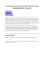
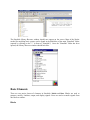
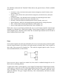
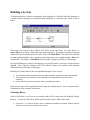
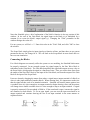
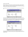
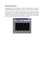
Power Electronics Laboratory
User Manual
Department of Electrical and Computer Engineering
Purdue University
Safety Precautions
General Precautions
•
Keep the work area neat and clean.
•
No object lying on table or nearby circuits.
•
Always use safety glasses when testing the circuit.
•
No loose wires or metal pieces should be lying on table or near the circuit, to cause shorts and
sparking.
•
Avoid using long wires, that may get in your way while making adjustments or changing leads.
•
Keep high voltage parts and connections out of the way from accidental touching and from any
contacts to test equipment or any parts, connected to other voltage levels.
•
When working with inductive circuits, reduce voltages or currents to near zero before switching
open the circuits.
•
BE AWARE of dangling objects like bracelets, rings, metal watch bands, and loose necklace (if
you are wearing any of them), they conduct electricity and can cause burns. Do not wear them
near an energized circuit.
•
When working with energized circuits (while operating switches, adjusting controls, adjusting
test equipment), use only one hand while keeping the rest of your body away from conducting
surfaces.
Before Powering the Circuit
•
Check for all the connections of the circuit and scope connections before powering the circuit, to
avoid shorting or any ground looping, that may lead to electrical shocks or damage of equipment.
•
Check any connections for shorting two different voltage levels.
•
Check if you have connected load at the output.
•
Double check your wiring and circuit connections (use a point-to-point wiring diagram to review
when making these checks).
While Switching ON the Circuit
•
Apply low voltages or low power to check proper functionality of circuits.
•
Once functionality is proven, increase voltages or power, stopping at frequent levels to check for
proper functioning of circuit or for any components is hot or for any electrical noise that can
affect the circuit normal operation.
While Switching OFF the Circuit
•
Reduce the voltage or power slowly till it comes to zero.
•
Switch of all the power supplies and remove the power supply connections.
•
Let the load be connected at the output for some time, so that it helps to discharge capacitor or
inductor if any, completely.
While Modifying the Circuit
•
Switch Off the circuit.
•
Modify the connections based on the requirement.
•
Recheck the circuit and switch ON.
Simulink Basics Tutorial
Starting Simulink
Basic Elements
Building a System
Running Simulations
Simulink is a graphical extension to MATLAB for the modeling and simulation of systems. In
Simulink, systems are drawn on screen as block diagrams. Many elements of block diagrams are
available (such as transfer functions, summing junctions, etc.), as well as virtual input devices
(such as function generators) and output devices (such as oscilloscopes). Simulink is integrated
with MATLAB and data can be easily transferred between the programs. In this tutorial, we will
introduce the basics of using Simulink to model and simulate a system.
The idea behind these tutorial is that you can view it in one window while running
Simulink in another window. Do not confuse the windows, icons, and menus in the
tutorials for your actual Simulink windows. Most images in these tutorials are not
live - they simply display what you should see in your own Simulink windows. All
Simulink operations should be done in your Simulink windows.
Starting Simulink
Simulink is started from the MATLAB command prompt by entering the following command:
>>simulink
Alternatively, you can click on the "Simulink Library Browser" button at the top of the MATLAB
command window as shown below:
The Simulink Library Browser window should now appear on the screen. Most of the blocks
needed for modeling basic systems can be found in the subfolders of the main "Simulink" folder
(opened by clicking on the "+" in front of "Simulink"). Once the "Simulink" folder has been
opened, the Library Browser window should look like:
Basic Elements
There are two major classes of elements in Simulink: blocks and lines. Blocks are used to
generate, modify, combine, output, and display signals. Lines are used to transfer signals from
one block to another.
Blocks
The subfolders underneath the "Simulink" folder indicate the general classes of blocks available
for us to use:
•
•
•
•
•
•
•
•
Continuous: Linear, continuous-time system elements (integrators, transfer functions, statespace models, etc.)
Discrete: Linear, discrete-time system elements (integrators, transfer functions, state-space
models, etc.)
Functions & Tables: User-defined functions and tables for interpolating function values
Math: Mathematical operators (sum, gain, dot product, etc.)
Nonlinear: Nonlinear operators (coulomb/viscous friction, switches, relays, etc.)
Signals & Systems: Blocks for controlling/monitoring signal(s) and for creating subsystems
Sinks: Used to output or display signals (displays, scopes, graphs, etc.)
Sources: Used to generate various signals (step, ramp, sinusoidal, etc.)
Blocks have zero to several input terminals and zero to several output terminals. Unused input
terminals are indicated by a small open triangle. Unused output terminals are indicated by a
small triangular point. The block shown below has an unused input terminal on the left and an
unused output terminal on the right.
Lines
Lines transmit signals in the direction indicated by the arrow. Lines must always transmit signals
from the output terminal of one block to the input terminal of another block. One exception to
this is that a line can tap off of another line. This sends the original signal to each of two (or
more) destination blocks, as shown below:
Lines can never inject a signal into another line; lines must be combined through the use of a
block such as a summing junction.
A signal can be either a scalar signal or a vector signal. For Single-Input, Single-Output systems,
scalar signals are generally used. For Multi-Input, Multi-Output systems, vector signals are often
used, consisting of two or more scalar signals. The lines used to transmit scalar and vector
signals are identical. The type of signal carried by a line is determined by the blocks on either
end of the line.
Building a System
To demonstrate how a system is represented using Simulink, we will build the block diagram for
a simple model consisting of a sinusoidal input multiplied by a constant gain, which is shown
below:
This model will consist of three blocks: Sine Wave, Gain, and Scope. The Sine Wave is a
Source Block from which a sinusoidal input signal originates. This signal is transferred through
a line in the direction indicated by the arrow to the Gain Math Block. The Gain block modifies
its input signal (multiplies it by a constant value) and outputs a new signal through a line to the
Scope block. The Scope is a Sink Block used to display a signal (much like an oscilloscope).
We begin building our system by bringing up a new model window in which to create the block
diagram. This is done by clicking on the "New Model" button in the toolbar of the Simulink
Library Browser (looks like a blank page).
Building the system model is then accomplished through a series of steps:
1. The necessary blocks are gathered from the Library Browser and placed in the model window.
2. The parameters of the blocks are then modified to correspond with the system we are
modelling.
3. Finally, the blocks are connected with lines to complete the model.
Each of these steps will be explained in detail using our example system. Once a system is built,
simulations are run to analyze its behavior.
Gathering Blocks
Each of the blocks we will use in our example model will be taken from the Simulink Library
Browser. To place the Sine Wave block into the model window, follow these steps:
1. Click on the "+" in front of "Sources" (this is a subfolder beneath the "Simulink" folder) to display
the various source blocks available for us to use.
2. Scroll down until you see the "Sine Wave" block. Clicking on this will display a short explanation
of what that block does in the space below the folder list:
3. To insert a Sine Wave block into your model window, click on it in the Library Browser
and drag the block into your workspace.
The same method can be used to place the Gain and Scope blocks in the model window. The
"Gain" block can be found in the "Math" subfolder and the "Scope" block is located in the "Sink"
subfolder. Arrange the three blocks in the workspace (done by selecting and dragging an
individual block to a new location) so that they look similar to the following:
Modifying the Blocks
Simulink allows us to modify the blocks in our model so that they accurately reflect the
characteristics of the system we are analyzing. For example, we can modify the Sine Wave
block by double-clicking on it. Doing so will cause the following window to appear:
This window allows us to adjust the amplitude, frequency, and phase shift of the sinusoidal
input. The "Sample time" value indicates the time interval between successive readings of the
signal. Setting this value to 0 indicates the signal is sampled continuously.
Let us assume that our system's sinusoidal input has:
•
•
•
Amplitude = 2
Frequency = pi
Phase = pi/2
Enter these values into the appropriate fields (leave the "Sample time" set to 0) and click "OK" to
accept them and exit the window. Note that the frequency and phase for our system contain 'pi'
(3.1415...). These values can be entered into Simulink just as they have been shown.
Next, we modify the Gain block by double-clicking on it in the model window. The following
window will then appear:
Note that Simulink gives a brief explanation of the block's function in the top portion of this
window. In the case of the Gain block, the signal input to the block (u) is multiplied by a
constant (k) to create the block's output signal (y). Changing the "Gain" parameter in this
window changes the value of k.
For our system, we will let k = 5. Enter this value in the "Gain" field, and click "OK" to close
the window.
The Scope block simply plots its input signal as a function of time, and thus there are no system
parameters that we can change for it. We will look at the Scope block in more detail after we
have run our simulation.
Connecting the Blocks
For a block diagram to accurately reflect the system we are modeling, the Simulink blocks must
be properly connected. In our example system, the signal output by the Sine Wave block is
transmitted to the Gain block. The Gain block amplifies this signal and outputs its new value to
the Scope block, which graphs the signal as a function of time. Thus, we need to draw lines from
the output of the Sine Wave block to the input of the Gain block, and from the output of the Gain
block to the input of the Scope block.
Lines are drawn by dragging the mouse from where a signal starts (output terminal of a block) to
where it ends (input terminal of another block). When drawing lines, it is important to make sure
that the signal reaches each of its intended terminals. Simulink will turn the mouse pointer into
a crosshair when it is close enough to an output terminal to begin drawing a line, and the pointer
will change into a double crosshair when it is close enough to snap to an input terminal. A signal
is properly connected if its arrowhead is filled in. If the arrowhead is open, it means the signal is
not connected to both blocks. To fix an open signal, you can treat the open arrowhead as an
output terminal and continue drawing the line to an input terminal in the same manner as
explained before.
Properly Connected Signal
When drawing lines, you do not need to worry about the path you follow. The lines will route
themselves automatically. Once blocks are connected, they can be repositioned for a neater
appearance. This is done by clicking on and dragging each block to its desired location (signals
will stay properly connected and will re-route themselves).
After drawing in the lines and repositioning the blocks, the example system model should look
like:
In some models, it will be necessary to branch a signal so that it is transmitted to two or more
different input terminals. This is done by first placing the mouse cursor at the location where the
signal is to branch. Then, using either the CTRL key in conjunction with the left mouse button
or just the right mouse button, drag the new line to its intended destination. This method was
used to construct the branch in the Sine Wave output signal shown below:
The routing of lines and the location of branches can be changed by dragging them to their
desired new position. To delete an incorrectly drawn line, simply click on it to select it, and hit
the DELETE key.
Running Simulations
Now that our model has been constructed, we are ready to simulate the system. To do this, go to
the Simulation menu and click on Start, or just click on the "Start/Pause Simulation" button in
the model window toolbar (looks like the "Play" button on a VCR). Because our example is a
relatively simple model, its simulation runs almost instantaneously. With more complicated
systems, however, you will be able to see the progress of the simulation by observing its running
time in the the lower box of the model window. Double-click the Scope block to view the output
of the Gain block for the simulation as a function of time. Once the Scope window appears,
click the "Autoscale" button in its toolbar (looks like a pair of binoculars) to scale the graph to
better fit the window. Having done this, you should see the following: