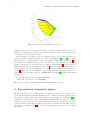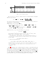
1
The Making of a Geometric Algebra Package in Matlab Computer Science Department University of Waterloo Research Report CS-99-27 Stephen Mann∗, Leo Dorst†, and Tim Bouma† [email protected], [email protected], [email protected] Abstract In this paper, we describe our development of GABLE, a Matlab implementation of the Geometric Algebra based on C`p,q (where p + q = 3) and intended for tutorial purposes. Of particular note are the matrix representation of geometric objects, effective algorithms for this geometry (inversion, meet and join), and issues in efficiency and numerics. 1 Introduction Geometric algebra extends Clifford algebra with geometrically meaningful operators, and its purpose is to facilitate geometrical computations. Present textbooks and implementation do not always convey this geometrical flavor or the computational and representational convenience of geometric algebra, so we felt a need for a computer tutorial in which representation, computation and visualization are combined to convey both the intuition and the techniques of geometric algebra. Current software packages are either Clifford algebra only (such as CLICAL [9] and CLIFFORD [1]) or do not include graphics [6], so we decide to build our own. The result is GABLE (Geometric Algebra Learning Environment) a hands-on tutorial on geometric algebra that should be accessible to the second year student in college [3]. The GABLE tutorial explains the basics of Geometric Algebra in an accessible manner. It starts with the outer product (as a constructor of subspaces), then treats the inner product (for perpendilarity), and moves via the geometric product (for invertibility) to the more geometrical operators such as projection, rotors, meet and join, and end with to the homogeneous model of Euclidean space. When the student is done he/she should be able to do simple Euclidean geometry of flats using the geometric algebra of homogeneous blades. Our desire to visualize meant that we did not need to go beyond 3 dimensions, and our implementation focuses on C`3,0 (although our implementation is general enough to handle other signatures in 3-dimensional space as well). Since this software is meant for a tutorial, we did not have great efficiency concerns (though we did have some), and were most interested in ease of implementation and the creation of a software package that could be made widely available. These goals led us to implement GABLE in Matlab, and to foster distribution of geometric algebra, it was made to work with the student version of Matlab. This paper describes our experiences in developing the package. We ran into some issues that any implementer of geometric algebra will need to decide on (representation, computational efficiency, stability of inverses); but we also encountered insufficiently precisely resolved issues in the very structure of geometric algebra itself, which the need for ∗ Computer † Computer Science Department, University of Waterloo, Waterloo, ON N2L 3G1, CANADA Science Department, University of Amsterdam, Kruislaan 403, 1098SJ Amsterdam, The Netherlands 1 2 The Making of a Geometric Algebra Package in Matlab Figure 1: Interpolation of orientations for a bivector. straightforward practical use brought out. Among these are the various inner products, and the precise definition and semantics of the meet and join operators in Euclidean geometry. This paper motivates and documents our decisions in these matters. Our representation of geometric objects is a refinement of the 8 × 8 representation that has been presented by others, along the lines suggested by Lounesto and Ablamowicz [8]pg 72), [1]. We compare this representation of geometric algebra to matrix representations of Clifford Algebras in Section 2. For the important but potentially expensive operation of inversion (or geometric division), we settled on a variation of a method proposed by Lounesto for C`3,0 , which we extend in Section 3 to work for arbitrary signature (in 3 dimensions). At the higher level, Section 4 gives some detail on our implementation of the meet and join operations, extending them to the non-trivial cases of partially overlapping subspaces. Section 5 discusses some of the peculiarities of doing all this in Matlab, the graphics portion of our package, and some of the numerical aspects of GABLE. The tutorial itself [3] is available on the World Wide Web at http://www.wins.uva.nl/~leo/clifford/gable.html http://www.cgl.uwaterloo.ca/~smann/GABLE/ These webpages contain both the Matlab package GABLE and the tutorial textbook. 2 Representation of geometric algebra The first decision we faced in our implementation was which representation to use for the geometric objects. The most natural representation in Matlab would be a matrix representation. Matrix representations for the geometric product in the Clifford algebras of various signatures are well studied [10]; for each signature a different matrix algebra results. That is slightly unsatisfactory. Moreover, our desire to make our algebra a proper geometric algebra implies that we should not only represent the geometric product, but also the outer and inner products, and preferably on a par with each other. These issues are discussed in more detail in Section 2.4; in brief, we ended up using a modified form of the 8 × 8 matrix representation. Mann, Dorst, Bouma – University of Waterloo Research Report CS-99-27 2.1 3 The matrix representation of GABLE In GABLE, we represent a multivector A as an 8 × 1 column matrix giving its coefficients relative to a basis for the Clifford algebra: A = [1, e1 , e2 , e3 , e1 ∧e2 , e2 ∧e3 , e3 ∧e1 , e1 ∧e2 ∧e3 ] A0 A1 A2 A3 A12 A23 A31 A123 , where {e1 , e2 , e3 } form an orthogonal basis for the vector space of our algebra. We will use bold font for the multivector, and math font for its scalar-valued coefficients. The multivector A is thus represented by an 8 × 1 column matrix [A], which we will denote in shorthand as A * ) [A]. Now if we need to compute the geometric product AB, we view this as a linear function of B determined by A, i.e., as the linear transformation AG (B), the ‘G’ denoting the geometric product. Such a linear function can be represented by an 8 × 8 matrix, determined by A (and the fact that we are doing a geometric product) acting on the 8 × 1 matrix of [B]. We thus expand the representation [A] of A to the 8 × 8 geometric product matrix [AG ], and apply this to the 8 × 1 representation[B] of B: G AB * ) [A ] [B]. The result of the matrix product [AG ][B] is the 8×1 matrix representing the element AB. The matrix entry [AG ]α,β (so in column α and row β, with α and β running through the indices {0, 1, 2, 3, 12, 23, 31, 123}) can be computed in a straightforward manner from the multiplication table of the geometric product: eα eβ = c eγ [AG ]γ,β = c Aα . ⇐⇒ (1) This 8 × 8 matrix [AG ] can then be used to evaluate the (bilinear) product AB by applying it to the 8 × 1 column matrix [B] using the usual matrix multiplication: [AB]γ = [AG ] [B] γ = X [AG ]γ,β [B]β . β So for example the identity e1 e2 = e12 leads to the matrix entry [AG ]12,2 = A1 ; this is the only nonzero entry in column β = 2. In matrix multiplication between A = A1 e1 and B = B2 e2 this yields [AB]12 = [AG ]12,2 [B]2 = A1 B2 , which is the correct contribution to the e12 component of the result. In algebraic parlance, the numbers c defined above (which depend on α, β and γ) are the structure coefficients of the algebra determined by the geometric product. In particular, each c will be a positive or negative factor depending on the basis of the algebra, the permutation of the elements, and the signature of the algebra. Both the outer and the inner product can be implemented as matrix multiplications, since A ∧ B and A · B are also linear functions of B, determined by A. So we implement O I A∧B * ) [A ] [B] and A · B * ) [A ] [B]. The 8 × 8 matrices [AO ] and [AI ] are given below, and they are constructed according to Equation 1 for the outer product and inner product, respectively. 4 The Making of a Geometric Algebra Package in Matlab 2.2 The representation matrices With the recipe of Equation 1, we now present the actual matrices. The c values of Equation 1 contain signed products of σi s. These represent the signature (and metric) through their definition as σi ≡ ei ei . Geometric product matrix: G [A ] = A0 A1 A2 A3 A12 A23 A31 A123 σ1 A1 A0 −σ1 A12 σ1 A31 −A2 σ1 A123 A3 A23 σ2 A2 σ2 A12 A0 −σ2 A23 A1 −A3 σ2 A123 A31 σ3 A3 −σ3 A31 σ3 A23 A0 σ3 A123 A2 −A1 A12 −σ1 σ2 A12 −σ2 A2 σ1 A1 −σ1 σ2 A123 A0 −σ1 A31 σ2 A23 A3 −σ2 σ3 A23 −σ2 σ3 A123 −σ3 A3 σ2 A2 σ3 A31 A0 −σ2 A12 A1 −σ1 σ3 A31 σ3 A3 −σ3 σ1 A123 −σ1 A1 −σ3 A23 σ1 A12 A0 A2 −σ1 σ2 σ3 A123 −σ2 σ3 A23 −σ1 σ3 A31 −σ1 σ2 A12 σ3 A3 σ1 A1 σ2 A2 A0 (2) Outer product matrix: O [A ] = A0 A1 A2 A3 A12 A23 A31 A123 0 A0 0 0 −A2 0 A3 A23 0 0 A0 0 A1 −A3 0 A31 0 0 0 A0 0 A2 −A1 A12 0 0 0 0 A0 0 0 A3 0 0 0 0 0 A0 0 A1 0 0 0 0 0 0 A0 A2 0 0 0 0 0 0 0 A0 (3) Inner product matrix: I [A ] = A0 0 0 0 0 0 0 0 σ1 A1 A0 0 0 0 0 0 0 σ2 A2 0 A0 0 0 0 0 0 σ3 A3 0 0 A0 0 0 0 0 −σ1 σ2 A12 −σ2 A2 σ1 A1 0 A0 0 0 0 −σ2 σ3 A23 0 −σ3 A3 σ2 A2 0 A0 0 0 −σ3 σ1 A31 σ3 A3 0 −σ1 A1 0 0 A0 0 −σ1 σ2 σ3 A123 −σ2 σ3 A23 −σ1 σ3 A31 −σ1 σ2 A12 σ3 A3 σ1 A1 σ2 A2 A0 (4) Note the relation between these matrices: the inner product matrix and the outer product matrix both have all non-zero elements taken from the geometric product matrix. Note also the lack of signature in the outer product matrix; this is in agreement with the fact that it forms a (non-metric) Grassmann algebra that may be viewed as a geometric algebra of null vectors, for which all σi equal 0. The reader acquainted with geometric algebra may realize that we have implemented an inner product that differs slightly from Hestenes’ inner product [4]: we prefer the contraction defined in [7], since we found that its geometric semantics is much more convenient. We will motivate this in Section 4.3. We have implemented other inner products as well (see next section), but the contraction is the default. 2.3 The derived products It is common to take the geometric product as basic, and define the other products using it by selecting appropriate grades. This can be the basis for an implementation; the Maple package at Cambridge [6] has been so constructed. For our comparative discussion below, we state the definitions; these can be used in a straightforward manner to derive the matrix representations. Mann, Dorst, Bouma – University of Waterloo Research Report CS-99-27 q=0 p=0 p=1 p=2 p=3 p=4 IR(1) IR(1) IR(2) C(2) IH(2) 2 q=1 C(1) IR(2) 2 IR(2) IR(4) C(4) q=2 q=3 IH(1) C(2) IR(4) 2 IR(4) IR(8) 2 5 IH(1) IH(2) C(4) IR(8) C(8) Table 1: Matrix representations of Clifford algebras of signatures (p, q). Notation: IR(n) are n × n real matrices, C(n) are n × n complex-valued matrices, IH(n) are n × n quaternion-valued matrices, 2IR(n) are ordered pairs of n × n real matrices (which you may think of as a block-diagonal 2n × 2n matrix containing two real n×n real matrices on its diagonal and zeroes elsewhere), and similarly for the other number systems. • Outer product A∧B= X hhAir hBis is+r . (5) r,s where h·ir is the grade operator taking the part of grade r of a multivector. • Contraction inner product AcB = X hhAir hBis is−r , (6) r,s where the grade operator for negative grades is zero (we thank Svenson [11] for this way of writing the contraction). Note that this implies that ‘something of higher grade cannot be contracted onto something of lower grade’. For scalar α and a general non-scalar multivector A we get αcA = αA and Acα = 0. • Modified Hestenes inner product This is a variation of the Hestenes inner product that fixes its odd behavior for scalars (which messes up the meet operation, as discussed in Section 4.3): A ·M B = X hhAir hBis i|s−r| . (7) r,s For scalar α and a general non-scalar multivector A we get α ·M A = αA = A ·M α. • Hestenes inner product The original Hestenes product differs from Equation 7 in that the contributions of the scalar parts of A and B are explicitly set to zero. Note that mixed-grade multivectors require expansion of a double sum in all these products. 2.4 Representational issues in geometric algebra For Clifford algebras of arbitrary signature (p, q) (which means p + q spatial dimensions, of which p basis vectors have a positive square, and q have a negative square) linear matrix representations have long been known. We repeat part of the table of such representations in Table 1, see [10]. The various representations are non-equivalent, so the table can be used for arguments on unique representations. Note that the Clifford algebras for a 3-dimensional space can have many different representations depending on the signature. Though this is not a problem for implementations, it makes it harder to obtain a parametric overview on the metric properties of the various spaces, and a representation that contains the signature as parameters σi has our slight preference. The outer product forms a Grassmann algebra. We have been unable to find a similar representation table in the literature on Grassmann algebras, but at least for even-dimensional Grassmann algebras 6 The Making of a Geometric Algebra Package in Matlab this is easily established. A Clifford algebra with signature (p, p) can be converted into a 2p-dimensional Grassmann algebra by pairing of the basis vectors with positive and negative signature. The table then shows that the Grassmann algebra of even dimension p is isomorphic to IR(2p ). Odd dimensions can be seen as subalgebras of the next even dimension. The inner product is not associative, and is therefore not isomorphic to a matrix algebra. Our initial exclusive interest in C`3,0 suggests the representation C(2), with elements represented as (A0 + A3 ) + i(A12 + A123 ) (A1 − A31 ) + i(A2 + A23 ) (A1 + A31 ) + i(−A2 + A23 ) (A0 − A3 ) + i(−A12 + A123 ) , but this works only for the geometric product; the other products would then have to be implemented using the grade operator. We prefer a representation in which all three products are representable on a par, and in which signatures are parameterized. This desire to represent arbitrary signatures parametrically necessitates viewing C`3,0 as a subalgebra of C`3,3 , and therefore to choose a representation in IR(8). This algebra IR(8) also contains a representation of the outer product as a certain kind of lowertriangular matrices (in fact, Equation 2 works nicely: the matrix product of two such matrices faithfully represents the outer product). For arbitrary signatures, there cannot exist a change of representation in which both the outer product matrices and the geometric product matrices could be reduced to a smaller size (i.e., brought onto a block-diagonal representation of the same kind), since we need the full IR(8) to handle those signatures anyway. Now the need to represent the inner product as well indicates that we can not represent the elements of the algebra by matrices in their function as both operator (i.e., first factor) and operand (i.e., second factor). We therefore switch to the view where each product is seen as a linear function of the operand, parameterized by the operator, as detailed in Section 2.1. We maintain the IR(8)-representation of these linear functions, but they now operate on 8-dimensional vectors representing the operand (rather than forming an algebra of operators). Thus we arrive at the representation we have chosen (also for the geometric product), with the operator matrices naturally defined as in Equation 1. It should be clear that the same reasoning suggests an IR(2n ) representation of the geometric algebra of n-dimensional space of arbitrary signatures, with matrices defined for the three products in the same way. 2.5 Computational efficiency If we would represent our objects as 8 × 8 matrices of reals, the resulting matrix multiply to implement the geometric product would cost 512 multiplications and 448 additions. Further, using the 8 × 8 matrix representation, to compute the outer product and/or inner product, we would have to use the grade operator (or, for the outer product, pay the expansion cost to convert to the outer product 8 × 8 matrix representation). Addition and scalar multiplication of elements in this form require 64 additions and 64 multiplications respectively. This method is extremely inefficient and we will not discuss it further. The computational efficiency of the 8 × 1 format is better. Addition and scalar multiplication of elements in this form require 8 additions and 8 multiplications respectively. For the products, our method has the computational cost of having to expand one of the one of the 8 × 1 matrices to an 8 × 8 matrix and then multiply it by an 8 × 1 matrix at a cost of 64 multiplications, 56 additions, and the cost of expansion. When we include the cost of signatures in the expansion cost, then the total cost is increased by 48 multiplications. It is of course possible to use the table of Clifford algebra isomorphisms as a literal guide to the implementation. Let us consider the costs of implementing the special case of the 3-dimensional Clifford algebras; our table shows that this involves implementation of C(2), 2IR(2) and 2IH(1). In all representations the operations of addition and scalar multiplication have take 8 floating point additions and 8 Mann, Dorst, Bouma – University of Waterloo Research Report CS-99-27 a∧b 0 1 2 3 0 0 1 2 3 1 1 2 3 (4) 2 2 3 (4) (5) 7 3 3 (4) (5) (6) Table 2: Grade of the outer product of blades. Along the top row and left column are the grades of blades a and b; the table gives the grade of the outer product of these blades. Note that if the grade is greater than 3, then the result will be 0. floating point multiplications, respectively (in the IR(8) representation, these operations are performed on the 8 × 1 matrices representing the objects). To compute the geometric product we need to multiply elements. The complexity of the basic multiplications is: one complex multiply takes 4 floating point multiplications and 2 additions – we denote this as (4, 2); one double real multiply takes (2, 0); one quaternion multiply takes (16, 12). For a full matrix implementation to produce the geometric product this yields for C(2) a complexity of (32, 16); for 2IR(2) a complexity of (16, 8); for 2IH(1) a complexity of (32, 24). Depending on the structure of the algebra, one may thus be fortunate by a factor of two. These should be compared to our IR(8) implementation acting on 8 × 1 matrices, which has a complexity of (110, 56), for general signatures. This is a factor of 3 worse than 2IH(1), the most expensive of the other three representations. If we consider only C`3,0 , then we have no signature cost, and IR(8) costs (64, 56) compared to (32, 16) for C(2). To implement a full geometric algebra, these specific geometric product implementations need to be augmented with a grade operation to extract elements of the grade desired, according to Equations 6 and 5. For C(2) it takes (0, 8) to extract the eight separate elements, and presumably the same for 2IH(1) and 2IR(2). For simplicity of discussion, when extracting a single grade, we will assume that it costs 3 additions (although for scalars and trivectors, the cost is only 1 addition). This process of a geometric product followed by grade extraction is simple if the objects to be combined are blades (rather than general multivectors). Such an operation requires a geometric product followed by grade extraction, which for C(2) has a total worst case cost of (32, 19), although there may be some additional cost to test for the grade of the blade, etc., which would add (0, 16) to the cost ((32, 35) total) if we need to perform a full grade extraction of each operand. When taking the outer or inner product of multivectors that are not blades, the use of the geometric product and grade extraction becomes quite expensive, since we must implement a double sum (see Equations 5, 6, and 7). A naive implementation of this formula would require 16 geometric products and grade extractions, an additional 12 additions to combine the results for each grade, and 8 additions to reconstruction the result, for a total cost of (512, 324). However, looking at Table 2, we see that that six of these geometric products will always be 0, and we can easily rewrite our code to take advantage of this. This modification to the code reduces the cost to (320, 210). By unbundling the loop and simplifying the scalar cases (i.e., multiplying B by the scalar portion of A reduces 4 geometric products to one floating point addition (to extract the scalar) and 8 floating point multiplies, and multiplying A by the scalar portion of B reduces 3 more geometric products to one addition and 7 floating point multiplies) we can get the cost down to (32 ∗ 3 + 15, 19 ∗ 3 + 2 + 12 + 8) = (111, 79). Further special casing of the vector and bivector terms can reduce this cost to (33, 45) (as detailed in the next paragraph), but note that in doing this (a) we have left the complex representation for computing these products and (b) each product will need its own special case code. Regardless, the code that optimizes the product of each grade would cost (for the outer product) 16 additions for the initial grade extraction, 15 multiplies for the grade 0 cases, 6 multiplies and 3 additions 8 The Making of a Geometric Algebra Package in Matlab Operation addition scalar multiplication grade extraction geometric product other products of blades other products of multivectors 8×1 (0, 8) (8, 0) (0, 0) (64, 56) (64, 56) (64, 56) C(2) (0, 8) (8, 0) (0, 8) (32, 16) (32, 19) (111, 79) Table 3: Comparison of costs for 8 × 1 and C(2). Complex n×1 Geometric Product 2(3n+1)/2 22n Other products on blades 2(3n+1)/2 22n Other products on multivectors n2 2(3n+1)/2 22n Table 4: Comparison of costs of various methods, with n being the dimension of the underlying vector space. for each of the 3 vector/bivector cases, with the usual 12 additions for combining results and 8 more additions to reconstruct the complex number, giving a total cost of (33, 45). However, if we desire to write such special case code, we could do so for the 8 × 1 representation at the lower cost of (33, 9), since we would not have to extract and combine the grades to form our 8 × 1 representation. Note that the above discussion is on the cost of writing special case code for the outer product only. If we choose this route, we would also need to write special case code for each of the inner products and possibly for each dimensional space in which we wish to work. A reasonable compromise of special cases versus general code for the complex representation would be to handle the scalars as special cases and write the loops to avoid the combinations that will always give zero. Table 3 compares the costs of using the 8 × 1 representation and the C(2) representation, assuming we do the these optimizations for the C(2) products of multivectors. 2.5.1 Asymptotic costs If we are interested in arbitrary dimensional spaces, then we need to look at the asymptotic costs. Table 4 summarizes the costs of the complex and of the n × 1 representation (where n = p + q is the dimension of the underlying vector space) for the geometric product and for the other products on blades and for the other products on general multivectors. In this table, we only give the top term in the cost expression, ignoring grade extraction, etc., for the complex representation of other products. Use of only this top order term also ignores the savings achieved for the complex representation by not computing the products whose grade is higher than n and special casing the scalar products; such optimizations roughly equate to a factor of two savings. Note that we use the complex representation as a coarse representative of the other representations; in the other cases we would use the quaternion or double-real representation, which cost roughly a factor of 2 less than the complex representation. From the table, we see that asymptotically the complex representation is always best. However, for small n, the n × 1 representation is best when performing inner or outer products of general multivectors, with the cross-over point being around n = 14. But when n is 14, the cost of even the geometric product in the complex representation is extremely large, requiring roughly 3 × 10⁶ multiplications. For smaller n, the complex representation is better than the n × 1 representation for the geometric product and the products of blades, while the n × 1 representation is computationally less expensive than the complex representation for the other products of general multivectors. However the other products of general multivectors are rarely (if ever) performed in our present understanding of what Mann, Dorst, Bouma – University of Waterloo Research Report CS-99-27 constitute geometrically significant combinations. Thus, in general the complex/quaternion/double-real representation will be more efficient than the n × 1 representation by a factor of 2n/2 . The conclusion must be that once one has decided on a particular geometry for one’s application, reflected in a particular signature, it makes sense to implement it literally using the isomorphism of Table 1. These ratios of complexity hold for arbitrary dimension n: the IR(2n ) implementation has a complexity of 2n/2 times higher than the literal isomorphism implementation, depending on the algebra. The conclusion must be that once one has decided on a particular geometry for one’s application, reflected in particular signature, it makes sense to implement it literally using the isomorphism of Table 1. For the tutorial in 3 dimensional spaces, the cost of the 8 × 1 representation is only a factor of two more expensive than the complex representation. Since we were writing tutorial code, we felt this savings was more than offset by the explicitness of the signature. Also, the IR(8) representation was easier to code and debug than the C(2) would have been since the Aα coefficients appear explicitly in the IR(8) matrix, and we didn’t have to write any special product implementations that would be required to achieve better efficiency for the outer and inner products of general multivectors. Further, to implement the double-real or quaternion representations in Matlab would have required us to implement our own matrix multiply routine for those representations, which would have been far slower than using the 8 × 1 representation and the Matlab matrix multiply routines. 3 Inverses In Matlab, the obvious way to compute the inverse of a geometric object M is to express it in the 8 × 8 geometric product matrix representation, [M]. Then inversion of [M] may be done using the Matlab matrix inverse routine, and the first column of [M]−1 will be the representation of the inverse of M. However, when we implemented this method for computing the inverse, we found that it introduced small numerical errors on rather simple data, and thus was less stable than we would like. We investigated a method of Lounesto’s that was more stable in our testing, and is computationally considerably more efficient than a matrix inverse. Lounesto [8] (pg.57) proposes a method to compute inverses in Clifford algebras of 3-dimensional spaces. We discuss it now, and extend it slightly. Lounesto’s trick is based on the observation that in three dimensions (and that is essential!) the product of a multivector M and its Clifford conjugate M only has two grades, a scalar and a pseudoscalar (the Clifford conjugate is the grade involution of the reverse of a multivector). Let Mi denote the part of M of grade i, though we will write M0 for the scalar part. Then we compute MM = (M0 + M1 + M2 + M3 )(M0 − M1 − M2 + M3 ) = (M02 − M21 − M22 + M23 ) + 2(M0 M3 − M1 ∧ M2 ), and the first bracketed term is a scalar, the second a trivector. Further, at least in Euclidean 3-space, if such an object of the form ‘scalar plus trivector’ N0 + N3 is non-zero, then it has an inverse that is easily computed: (N0 + N3 )−1 = N0 − N3 . N02 − N23 Please note that not all multivectors have an inverse, not even in a Euclidean space: for instance M = 1 + e1 leads to MM = 0, so this M is non-invertible. In a non-Euclidean space, the denominator may become zero even when N0 and N3 are not, and we need to demand at least that N02 6= N23 . (When it exists, the inverse is unique. This follows using the associativity of the geometric product: if A and A0 are left and right inverses of B, respectively, then A = A(BA0 ) = (AB)A0 = A0 . Therefore any left inverse is a right inverse, and both are identical to the inverse.) 9 10 The Making of a Geometric Algebra Package in Matlab Term M MM −1 MM M(MM)−1 Total Naive (0,0) (64,56) 8×1 Good (0,0) (64,56) Scalar (0,0) (64,56) (4,1) (64,56) (132,113) (4,1) (16,8) (84,65) (0,0) (8,0) (72,56) Naive (0,8) (32,16) C(2) Good (0,8) (32,16) Scalar (0,8) (32,16) (4,1) (32,16) (64,41) (4,1) (16,8) (52,33) (0,0) (8,0) (40,24) Table 5: Cost of Lounesto’s inverse. These two facts can be combined to construct an inverse for an arbitrary multivector M (still in Euclidean 3-space) as follows: −1 M −1 = MM −1 M −1 = M(MM) = M (MM)0 − (MM)3 (MM)20 − (MM)23 The following two lemmas and their proofs demonstrate the correctness of Lounesto’s method in 3dimensional spaces of arbitrary signature. Lemma: 1 M−1 exists if and only if MM exists. Proof: First, assume that M−1 exists. Then 1 = M−1 M = (M−1 M−1 )(MM), so that (MM)−1 = M−1 M−1 , which exists. Secondly, assume that (MM)−1 exists. Then we have 1 = (MM)(MM)−1 = M(M(MM)−1 ), so that M−1 = M(MM)−1 , which exists. QED Lemma: 2 Let N = N0 + N3 . Then iff N02 6= N23 , N−1 exists and equals (N0 + N3 )−1 = N0 − N3 N02 − N23 Proof: Assume N02 6= N23 , then (N0 + N3 ) (N0 − N3 )/(N02 − N23 ) = (N02 + N3 N0 − N0 N3 − N23 )/(N02 − N3 )2 = (N02 − N23 )/(N02 − N23 ) = 1, so N−1 is as stated. Now assume that N−1 exists. Then if N3 = 0 the result is trivial. If N3 6= 0 and N0 = 0 the result is trivial. So take N3 6= 0 and N0 6= 0. Let K be the inverse of N = N0 + N3 . Then it needs to satisfy (N0 + N3 )(K0 + K1 + K2 + K3 ) = 1, so, written out in the different grades (N0 K0 + N3 K3 ) + (N0 K1 + N3 K2 ) + (N0 K2 + N3 K1 ) + (N0 K3 + N3 K0 ) = 1 Straightforward algebra on the terms of grade 0 and 3 yields (N02 − N23 )K3 + N3 = 0, and since N3 6= 0 this gives N02 6= N23 . Then the case above shows that the inverse is N−1 = (N0 − N3 )/(N02 − N23 ). QED Table 5 summarizes the costs to compute the inverse for both the 8 × 1 representation and for the C(2) representation. In this table, we give three algorithms for each representation: a naive algorithm, that does not try to exploit any extra knowledge we have about the terms we are manipulating; a good algorithm, that exploits the structure of (MM)−1 , which is a scalar plus a pseudo-scalar, and thus does not require a full product when multiplied by M; and a scalar version that can be used when (MM)−1 is a scalar. This last case occurs when M is a blade, a scalar plus a bivector, or a vector plus the pseudo-scalar, which covers most of the geometrically significant objects we manipulate. Mann, Dorst, Bouma – University of Waterloo Research Report CS-99-27 Note that in this table we have omitted the cost of the six negations needed to compute the Clifford conjugate. Also note that the complex representation requires 8 additions when computing the Clifford conjugate because it has to separate and recombine the scalar and pseudo-scalar part of the geometric object. Lounesto’s method is computationally much cheaper than the matrix inverse method, with a good implementation of Lounesto’s method requiring 149 Matlab floating point operations for the 8 × 1 representation, while the Matlab matrix inverse routine on 8 × 8 matrices requires 1440 Matlab floating point operations. Lounesto’s method really makes convincing use of the special structure of our matrices. While a faster matrix inversion routine may be available, it is unlikely that there will be a general routine capable of inverting our special 8 × 8 matrix in fewer than 149 floating point operations (which is after all little more than twice the number of matrix elements!). Further, in practice we found our modified Lounesto inverse to compute a more numerically stable inverse than the matrix inverse routine provided by Matlab (perhaps not surprising, since it involves fewer operations). Had we used the C(2) representation of elements in our geometric algebra, the cost of matrix inversion would have dropped dramatically, with Matlab requiring only 260 floating point operations to invert a 2×2 complex matrix. However, Lounesto’s method using the complex representation only requires 75 floating point operations. Thus Lounesto’s inversion method is also less expensive in the C(2) representation. 4 Meet and Join The geometric intersection and union of subspaces is done by the meet and join operations. These have mostly been used by others in the context of projective geometry, which has led to the neglect of some scalar factors and signs (since they do not matter in that application). This issue was partly treated in [2], but the development of the tutorial required some more investigation of those scalar factors. This section reports on that. 4.1 Definition The meet and join operations are geometrical ‘products’ of a higher order than the elementary products treated before. They are intended as geometrical intersection and union operators on (sub)spaces of the algebra. Since subspaces are represented by pure blades, these operations should only be applied to blades. Let blades A and B contain as a common factor a blade C of maximum grade (this is like a ‘largest common divisor’ in the sense of the geometric product), so that we can write A = A0 ∧ C and B = C ∧ B0 (note the order!). We will actually choose A0 and B0 to be perpendicular to C, so that we may also write the factorization in terms of the geometric product: A = A0 C and B = CB0 (but note that A0 and B0 are in general not mutually perpendicular!). If A and B are disjoint, then C is a scalar (a 0-blade). We now define meet and join as join(A, B) = A0 ∧ C ∧ B0 and meet(A, B) = C. Note that the factorization is not unique: we may multiply C by a scalar γ. This affects the join result by 1/γ and the meet by γ, so meet and join are not well-defined. (Since γ may be negative, not even the orientation of the results is defined unambiguously.) So these operations are hard to define in a Clifford algebra; but for a Geometric Algebra, they definitely desired. Many geometric constructions are actually insensitive to the magnitude and/or sign of the blade representing the subspace. A prime example is the projection (xcA)/A onto the subspace represented by A – there is not problem using for A the outcome of a meet or join. 11 12 The Making of a Geometric Algebra Package in Matlab In our implementation, we do want to guarantee that meet and join of the same subspaces can be used consistently, so we do need to base both on the same factorization. We can make the computational relationships between meet and join explicit. The definition gives for the join, given the meet (where the fraction denotes right-division): join(A, B) = A ∧ B. meet(A, B ) (8) Note that this is only valid if the meet is an invertible blade. In non-Euclidean spaces there may therefore be a problem with this equation and the factorization on which it is built: if C is a null blade (i.e., a blade with norm 0, non-invertible) then we cannot compute A0 in terms of A from the factorization equation A = A0 C, and therefore not compute join(A, B) = A0 ∧ B from the meet (or vice versa, by a similar argument). We thus have to limit join and meet to non-null blades; which means that we restrict ourselves to Euclidean spaces only. (Actually, anti-Euclidean spaces in which all signatures are −1 would obviously be permissible as well.) Since no blades are now null-blades, we can agree to make the common factor C a unit blade (so that |C| = 1) leaving only the sign of its orientation undetermined. But please be aware that this is a rather arbitrary partial fixing of the scalar factor! By duality relative to join(A, B) and symmetry of a scalar-valued contraction (or inner product) it follows from Equation 8 that 1= A B B A c = c . meet(A, B) join(A, B) join(A, B) meet(A, B) The division by meet(A, B) can be factored out (this is due to the containment relationship of the factors of the contraction and easy to prove using the techniques in [2]) and we obtain meet(A, B) = B c A. join(A, B) (9) Thus we can start from either meet or join and compute the other in a consistent manner. The symmetry of the equations means that either way is equally feasible.1 4.2 Implementation We saw that the three issues, factorization of A and B, computing their join (smallest containing superspace) and computing their meet (largest common subspace) are intertwined; giving any one determines the other two (at least in Euclidean signatures). We have chosen to use the join (i.e., the smallest common space of A and B) as the one to implement, and to base the meet on it using Equation 9. In principle, this determination of the smallest common space is a minimization problem, which may be solved by starting with a space that is too big and reducing it, or by growing one that is too small. In either case, the general case will involve some administration of polynomial time in the number of blades, and therefore exponential in the dimensionality of the space. We have not solved this general issue; in the 3-dimensional Euclidean space of interest in the tutorial the join is fairly easy to implement case by case. First observe that the definition implies that for disjoint spaces A and B, factored by a scalar C = 1, join(A, B) equals A ∧ B. In particular, we see in Table 6 that A ∧ B equals join(A, B) unless the dimensions of A and B are too high (sum exceeds 3), with some exceptional degeneracies when the grades are 1 and 2. So we may use the outer product as a basis for an algorithm. The table shows that of (B/I3 )cA may aid in treating some of the non-outer-product cases, where I3 is the pseudoscalar of our 3-dimensional Euclidean space (details below). This has led us to consider two algorithms for the computation of the join: 1 Equation 9 is frequently extended to provide a 3-argument meet function relative to a general blade I: meet(A, B, I) ≡ (B/I) · A. However, since the geometric significance of using anything but join(A, B) as third argument is unclear, we will not use it. Also, beware that some writers may switch the order of the arguments in this formula! Mann, Dorst, Bouma – University of Waterloo Research Report CS-99-27 join(A, B) 0 1 2 3 A∧B 0 1 2 3 0 0 1 2 3 1 1 2(∅) 3(∅) ∅ 2 2 3(∅) ∅ ∅ 3 3 ∅ ∅ ∅ 0 0 1 2 3 1 1 2(1) 3(2) 3 2 2 3(2) 3(2) 3 (B/I3 )cA 0 1 2 3 13 3 3 3 3 3 0 3 2 1 0 1 2 1(∅) 0(∅) 1 2 1 0(∅) 1(∅) 2 3 0 1 2 3 Table 6: The result of the join in 3-space can often be computed using the wedge product. We have indicated the grade of the results, with ∅ indicating a zero result, and results in brackets alternative outcomes in degenerate cases. • Algorithm A For non-degenerate arguments, we can implement join(A, B) by computing the quantity J = A∧B. If J is non-zero, then it is the result we want. Otherwise, if the grade of one of the arguments equals 3, the result is proportional to this argument. For instance, let grade (A) = 3, then a possible factorization of B is through B = Cβ (with B0 = β a scalar) which yields join(A, B) = A ∧ B0 = βA. If we choose the common factor to be a unit blade, then β = ±|B|, so that the result is join(A, B) = ±|B|A. We choose, arbitrarily, the positive sign. That leaves the exceptions. When not both grades are 2, the result is proportional to the argument of highest grade, by a scalar factor depending on the other argument (by the same reasoning as above, taking that scalar factor equal to the norm implies considering the common factor to be a unit blade). When both grades are 2, we need to find whether these 2-blades are coincident or not. If they are not, then their join is proportional to I3 , so we may use Equation 8 to compute a carrier for this common subspace: M = (B/I3 )cA. We normalize this to a unit blade: C = M/|M|, and then return join(A, B) = (A/C) ∧ B as the proper multiple of I3 . If they are coincident, the computation of M yields zero (which is how we may detect it) and we return |A|B or, equivalently up to the undetermined sign, |B|A. • Algorithm B For non-degenerate arguments, we can implement join(A, B) by computing the quantity J = A∧B. If J is non-zero, then it is the result we want. Otherwise, we compute M = (B/I3 )cA. If M is non-zero, then it is proportional to the meet (since precisely in those cases, the join is proportional to the blade I3 of grade 3). The common factor C is then the unit blade C = M/|M|, so the join is then A0 ∧ C ∧ B0 = (A/C) ∧ B. In the degenerate cases indicated in parentheses in the table for the join, both J and M of the previous paragraph are zero. Which degenerate case we have is readily determined by testing the grade of A and B. If both are vectors or bivectors, then they must be parallel. The factoring is thus A = αC and B = Cβ, with both α and β scalars. The result of the join is then join(A, B) = αβC = αB = βA. We can implement this as |A|B or |B|A, if we agree to factor out a unit blade C. If exactly one of A and B is a vector c, then the other must be a bivector containing this vector as a factor. The factorization is now A = ac and B = βc, so join(A, B) = βac = βA (if A is the bivector) or A = αc and B = cb, so join(A, B) = αB (if B is the bivector). If we fix the common 14 The Making of a Geometric Algebra Package in Matlab blade c to be a unit blade, this may be implemented as |B|A or |A|B, respectively. Algorithm A is computationally faster since it mostly does testing of grades to establish the exceptional cases. Algorithm B has a simpler conditional structure, leading to simpler code. It is the one we implemented. With the join found, the meet is computed from Equation 9. Although either is only determined only up to a scalar, they are consistent in the sense of those equations, and their relative magnitudes may therefore be used to derive geometrically meaningful results. 4.3 Why we use a contraction as inner product We gave three different inner product definitions in Section 2.3, and we still owe the explanation on why we prefer the contraction, which has been used so rarely in geometric algebra. The main reason is that Hestenes’ original inner product (abbreviated as HIP) has some features that make it less suitable for straightforward geometric interpretations. This shows up rather clearly when it is used in the meet operation, and in projection operations. The former can be fixed by treating the scalars differently, the latter requires more and leads to the contraction. Suppose we take the meet of I3 and a vector a, in the 3-dimensional space with pseudoscalar I3 . We would obviously expect the outcome to be a multiple of a, since the meet should have the semantics of geometric intersection, and the intersection of the subspace spanned by I3 and the subspace spanned by a should be the subspace spanned by a. The join of I3 with any subspace is I3 , so we may use Equation 9 to compute the meet. Using the Hestenes inner product, denoted as ·H , we obtain: meetH (a, I3 ) = (I3 /I3 ) ·H a = 1 ·H a = 0, since the HIP with a scalar is zero. On the other hand meetH (I3 , a) = (a/I3 ) ·H I3 = a. So the meetH is severely asymmetrical, which is unexpected for an operation that should be geometric intersection. In this case, it is due to the awkward properties of scalars (which [5] page 20 notes, but does not fix). We can fix this by modifying the Hestenes inner product to a new inner product denoted ·M , the same as ·H except for scalars. For scalars, we demand that α ·M u = α u for scalar α, and any multivector u. This leads to the modified Hestenes inner product defined in Equation 7. We will abbreviate it as modified HIP. For non-scalars this modified HIP has a certain symmetry in grades of the arguments: the inner product of a blade of grade r with one of grade s, or vice versa is a blade of grade |r − s|. The contraction of Equation 6 does not have this property: it actually ‘contracts’ the first argument inside the second, one cannot contract something of a bigger grade onto something of a smaller grade. For its use in the meet, this is a distinction without a difference, since in the evaluation of Equation 9 as (B/join(A, B))cA, the first argument blade of the inner product has a grade that never exceeds that of the second argument blade. But the selection of the inner product also has an effect on the evaluation of the projection. For blades, Hestenes and Sobczyk [5] define the projection of A into B as (A·H B)·H B−1 . Some problems with scalars are noted (see [5], page 20) which we can fix by using ·M instead. Using that but following the reasoning of [5], we can then show that the projection can be simplified to (A ·M B)/B if grade (A) ≤ grade (B), and zero otherwise. Rightly, [5] prefers the new algebraic form since it makes proofs easier. Yet there is still this conditional split into cases; when treating blades of grades not known a priori this may lead to lots of cases and still make work hard. Using the contraction, the projection onto the blade B can be defined as (AcB)/B, for all arguments A. This is automatically zero when A exceeds B; since the algebraic properties of the contraction are Mann, Dorst, Bouma – University of Waterloo Research Report CS-99-27 15 similar to those of the (extended) HIP, most proofs still work unchanged in their mechanics, but now do not require careful conditional splits dependent on the grades of the arguments complicating the reasoning. Geometrically interpreted, the contraction implicitly contains subspace relationships, in the sense that the blades resulting from the simple formula AcB must be contained in B, and so must the result of the division by B to produce the actual projection. This therefore encodes something that must be added as a separate concept when using the (modified) HIP: that subspaces may be contained inside each other; Hestenes’ conditions on the grade impose this explicitly; the contraction does it implicitly without additional structure, and thus provides a simpler algebra without sacrificing any geometry. In summary, the choice between HIP and modified HIP is clear: use the modified HIP or you will get a much more complicated geometric intersection operation as meet. It can probably be fixed with some grade testing, but this is not as elegant as fixing the inner product instead. Our preference for the contraction is based on the algebra and geometrical semantics that permits a simpler projection operator.2 Again, this can be fixed with appropriate grade testing, but we prefer the more straightforward modification of the inner product. The power of the meet and join defined in this way – making essential usage of the contraction – shows in the connection function in GABLE (see [3]): it is possible to give an algorithm without cases to compute the translation to make the meet between two affine subspaces non-trivial. Here ‘case-less’ means: no internal separate treatment of situations, all situations are computed using the same formula (whether point-to-point, line-to-line, line-to-point, parallel lines). Moreover, this formula is also valid in arbitrarily dimensional (Euclidean) space. The fact that we can do this shows that we are beginning to have the right primitive operations at our disposal in a computational language for geometry. 5 Implementation details This section describes some of the implementation details of GABLE. We include it so that others may benefit from our experiences. 5.1 Geometric algebra programming details We encountered a few issues with programming the geometric algebra that were not specific to Matlab. In particular, the use of coordinate frames and the inner product. 5.1.1 Frames Geometric algebra has the property of being “coordinate-free.” However, to read and write data, we are forced to use a coordinate system. We chose to use an orthonormal basis for the vector space ({e1 , e2 , e3 }), which we implemented as Matlab functions. By implementing these basis elements as functions, we avoided initialization problems, and they are globally available to all Matlab functions without having to explicitly declare them. We give the user the option to set the vector basis to be used for output. GABLE does not allow the user to select the bivector output basis or the pseudoscalar output basis; if a vector basis of ({a1 , a2 , a3 }) is used for the output of vectors, then we automatically select the basis {a1 ∧ a2 , a2 ∧ a3 , a3 ∧ a1 } for the output of bivectors, and a1 ∧ a2 ∧ a3 for the output of the pseudo-scalar. 2 It is of some concern that the contraction combines the notions of perpendicularity and containment in one operation (for AcB is contained in B and perpendicular to A), and we need to investigate whether the remainder of the structure of geometric algebra enables their disentanglement; the projection operation suggests that it does. We should also mention an alternative definition of the contraction, as the adjoint of the outer product in terms of an extension of the bilinear form, which demonstrates its basic algebraic tidiness (see [7]) and its nicely ‘dual’ relationship to the outer product. This makes for improved duality relationships, see [2]. 16 The Making of a Geometric Algebra Package in Matlab 5.1.2 Inner products As detailed earlier, we experimented with three inner products: the standard Hestenes inner product, the variation of Hestenes product for which scalars are multiplied rather than resulting in zero, and the Lounesto contraction. Although we found that the contraction was the most useful for our tutorial, we have made all three available as innerH, innerS, contraction respectively. The inner product routine itself, inner, is merely a routine that selects among the three inner products. To set a particular inner product, use GAitype, with 0 corresponding to the contraction, 1 to the Hestenes inner product, and 2 to the inner product that handles scalars. 5.2 Matlab objects The Matlab language has objects. For our implementation of the geometric algebra, we created a GA object, which stores the 8 × 1 matrix representing a geometric object. No other information is stored in the object. However, the benefit of using an object is that we were able to overload the ‘*’ and ‘ˆ’ operators to perform the geometric product and the inner product respectively. We also overloaded ‘+’ and ‘-’ (both binary and unary) to add, subtract, and negate geometric objects. Operations such as dual, inverse, and exponentiation we left as named routines (dual, inverse, and gexp respectively), although we did overload the ‘/’ operator to allow for right-division by a geometric object. I.e., the expression A/B is computed as A*inverse(B). We also overloaded ‘==’ and ‘~=’ to allow for the comparison of geometric objects. 5.3 Scalars Scalar values caused us several problems. Matlab represents these as type double. However, a GA object is a matrix of eight scalars. When all but the first entry are zero, the GA object represents a scalar. Rather than have the user explicitly convert from double to GA, our routines check their input for type double and automatically convert it to a GA scalar as needed. We also had to decide what to do if the results of one of our procedures was a scalar. Our choices were to leave this as a GA object, which facilitates certain internal choices and simplifies some code, or to automatically convert scalars back and forth between double and GA. We chose the latter approach, as it fits more naturally with the rest of Matlab and seems more appropriate for the tutorial setting. However, this automatic conversion interacts poorly with our overloading of the circumflex for the outer product. With automatic conversion of GA to double, if A and B in the expression A^B are both scalars, then both are converted to double and Matlab calls the scalar exponentiation function rather than our outer product function. Since the outer product of two scalars is actually the product of the two scalars, the result will be incorrect. For simple testing of the geometric algebra, the wedge product problem should not be a problem. However, if you are concerned, you can turn off automatic conversion of GA scalars to double by using the command GAautoscalar. Called with an argument of 0 turns off the auto-conversion, and called with an argument of 1 turns auto-conversion on. Alternatively, if you have a value v that must be a have a GA object and not a scalar, you may write GA(v). GAautoscalar does not affect the automatic conversion of arguments to our routines from double to GA scalars. Since checking the type of the arguments takes time, we have a set of internal routines that assume their arguments are of type GA and always leave their results as type GA. If you prefer to do the conversion manually, you may use this alternative set of routines; note, however, that you will be unable to use the overloaded operators. Table 7 summarizes the correspondence between the two sets of routines. To create a GA object from a scalar s, use GA(s). To convert a GA object g to a double, use double(g). Mann, Dorst, Bouma – University of Waterloo Research Report CS-99-27 Autoconvert * + ^ / dual 17 GA arguments GAproduct GAplus GAminus GAouter GAdivide GAdual Table 7: Correspondence between auto-conversion routines and GA routines 0.5 1 0.5 0.02 0 −0.02 0 0.5 0.5 0 0 −0.5 0 −0.5 −0.5 0.5 0 −0.5 0.5 0 −0.5 Figure 2: Graphical representation of vector, bivector, trivector One further complexity introduced by the autoconversion of scalars was a need for a non-GA version of our routines. In Matlab, if one or more arguments of a routine is an object, the system checks to see if that routine is a class method, and invokes that method if it is. However, if no arguments are objects, then the class methods are not considered. Thus, to handle scalars, we needed a function corresponding to most of our GA methods that handles the case when all arguments are scalars. For example, our draw routine needs to draw scalars. But if draw is given a scalar argument, the GA object method draw is not called. Thus, we wrote a second draw routine to handle the scalar case. 5.4 Graphics Since we wanted a visual tutorial, we created graphical representations for all blades, and used Matlab rendering commands to draw them. The following table summarizes our representations: Type Representation Orientation scalar vector bivector trivector Text above window Line from origin Disk centered at origin Line drawn sphere None Arrow head Arrows along edge Line segments going out or in Figure 2 illustrates the vector, bivector, and trivector; the axes are put in automatically by Matlab. We chose the disk as our representation for bivectors since with our matrix representation of the geometric objects, we do not necessarily have the defining vectors for the bivector (which may not even exist, as is the case if the bivector was created as the dual of a vector). Without such vectors, we can not use the standard parallelogram representation of the bivector. We had a similar problem with the trivector (i.e., we were unable to use a parallelepiped as its representation) and thus we used the 18 The Making of a Geometric Algebra Package in Matlab sphere. However, we also provide demonstration routines to illustrate the more standard representations of bivectors and trivectors, but the user must provide the basis on which to decompose them. Objects of mixed grade presented a more difficult problem. While it is easy to draw the scalar, vector, bivector, and trivector components independently, this is not particularly illustrative. We found it more useful to illustrate the operations of the inner, outer, and geometric products. The first two are fairly easy to demonstrate: we have two subwindows, in the former we draw the operands and in the latter we draw the result. The geometric product is more difficult to illustrate. So in addition to providing a routine to show the operands and result of the geometric product, we presented examples of using the geometric product as an operator to perform rotations and interpolation between orientations. Because of the peculiarities of our graphics routines (multiple windows with the same view, equal coordinate axes, etc.) we wrote our own routine (GAview) to change the Matlab view. Further, to help give the user a better grasp of the 3D scene, we wrote GAorbit, a variation on a Matlab sample routine for rotating the scene. The main difference between our viewing routines and the ones in Matlab is that our routines keep the same view on all subplots and using equal axes. 5.4.1 Matlab colors We considered several options for the rendering method. In particular, we considered allowing the user to have full shaded images of vectors, bivectors, etc. We discarded this idea, as it would have significantly added to the non-geometric algebra complexity of the tutorial, made our coding task harder, and for color mapped displays there would be problems similar to those discussed below. Not using shaded images does have a distinct disadvantage: the shading gives important depth cues that help the user determine the 3D aspects of the picture. However, we found that having a routine that rotates the scene (GAorbit in GABLE) gives sufficient depth cues to allow us to properly visualize the graphics. We also considered allowing (at least as an option) the user to specify colors as an RGB triple. While there are clear advantages to such an option (a larger range of colors available being the primary advantage), we again rejected it, partially because of the added complexity, but more so for color map reasons. On an 8-bit graphics display, only a limited number of colors (256) are available on the display at any one time, even though the monitor is capable of displaying a much larger range of colors. To give the user of an 8-bit display access to the full 24-bits of available colors, the windowing system creates a color map for each window that maps each 8-bit color value to a 24-bit color. Since several windows are visible at one time, many systems use the color map of the current window as the color map for the entire display. This use of the current window’s color map as the color map for the entire display would be disastrous for our Matlab application, since the user types in one window (which on many systems is the window whose color map is used for the display) and has the graphics displayed in another window. If the graphics window has its own color map, the user would have to type in one window, then switch contexts to the other window to see the proper colors. Such a change of contexts is difficult and leads to confusion, especially for inexperienced computer users. For the colors for our package, we chose to use the Matlab ASCII colors. Matlab uses a small set of characters to designate some basic colors as indicated in Table 8. To draw a geometric object in a particular color, you specify the color as an optional argument to our drawing routines. In addition, a few of our drawing routines have a color ’n’, which disables part of its drawing. In our experience with our geometric algebra package, we found that while we occasionally wanted additional colors and shading, we were able to illustrate everything we wanted with the ASCII colors that Matlab provides. Mann, Dorst, Bouma – University of Waterloo Research Report CS-99-27 Character Color ’r’ red ’g’ green ’b’ blue ’c’ cyan ’m’ magenta ’y’ yellow 19 ’k’ black ’w’ white Table 8: Matlab colors One common graphics feature that Matlab lacks is transparency, which would have been extremely useful to us to show things behind or inside of objects. For example, if we had transparency, then we would have rendered a trivector as a transparent sphere rather than a line drawing of a sphere. However, it is likely that transparency would have had the color map problems discussed above, and that we at least would have needed an option to shut it off. 5.4.2 Matlab graphics problems The Matlab hold, axis, and rendering methods interacted poorly with our package. The following summarizes how we overrode Matlab’s defaults and why: • axis. To properly display the arrow heads of our vectors, we need equally scaled axes. If we have non-uniform scaling, the arrow heads look like open umbrellas, and further no longer appear perpendicular to the arrow body itself. To force equal axes, in the draw command we call axis(’equal’). If you want non-uniform scaling of your axes, you will need to make a call to axis after your last call to draw. The problems are worse for GAorbit, especially when drawing multiple subgraphs. GAorbit sets axis vis3d, and rotates all subgraphs simultaneously. Further, DrawOuter, etc., call a routine that finds the min/max of all the subgraph axes (being careful of 2D plots) and sets all subplots to have the same axis. • hold. We use the patch command to draw some of our objects and plot3 command to draw other objects, and some objects are drawn with both. Matlab appears to call ‘hold on’ when patches are drawn, but does not make such a call when drawing lines. To make our drawing routines behave consistently for all geometric objects, we call ‘hold on’ at various places internal to our routines. • render. There are two rendering modes: ’painter’ and ’zbuffer’. Unfortunately, the painter mode does not split overlapping polygons. Since all our bivectors overlap, drawing two bivectors in painter mode draws one completely on top of the other, which is incorrect. Thus, we set the default rendering mode to ’zbuffer’, which correctly renders the bivectors. However, when saving the graphics screen to a PostScript file (such as for making figures), if you’ve rendered with the ‘zbuffer’ mode Matlab creates a bitmap image, which is huge and of low quality. If you’re using the ’painter’ rendering mode, Matlab will create a smaller, more reasonable PostScript file. If there is only one bivector in your image, this latter method is preferred. To allow for both, we wrote a GArender command. With no arguments, it returns the current rendering mode. With one argument, it sets the rendering mode to that argument. 5.5 Dealing with numerical issues Numerically, some routines (particularly the inverse routine) may create small error terms. For example, we might get a Geometric Object that should be a vector, but has a small (on the order of 10−16 ) bivector term. Several of our routines (e.g., the drawing routines) check to make sure that the arguments are blades, and such numerical errors, though small, will cause these routines to fail. I.e., while the numerical error causes no particular computational problems, some routines will reject such geometric objects as not being blades. Thus, we wrote gazv, which sets all small terms of a geometric object to zero. 20 The Making of a Geometric Algebra Package in Matlab The routine gazv will set to zero all terms of a GA that are smaller in absolute value than 1e-15, giving a warning when it does so. When developing code, it is a good idea to use gazv to overcome small numerical problems, and once the code is debugged switch to grade (since presumably you know the grade you want). Although you could use grade from the beginning, its use might hide some bugs that the system would otherwise automatically catch for you. We additionally wrote two similar routines: GAZ, which is identical to gazv except that it doesn’t produce a warning message, and blade which converts a geometric object into a blade. Since this software is meant for a tutorial, our == and = operators compare to within a numerical tolerance. Thus, vectors, etc., differing by only small amounts will be considered equal. If an exact equality is desired, one may use the eeq function. Any further testing will require extracting the coordinates using inner. Other than these small round-off errors (usually introduced by inverse), we encountered no numerical problems with GABLE. However, it should be noted that we did not perform extremely complex computations, and further testing of our software is needed to better assess its numerical stability. 5.6 Hacking To implement the basic geometric algebra, we used the following “hacks”: • We wanted the canonical basis vectors e1, e2, and e3 to be available as global variables without having to declare them in each function (i.e., like pi in Matlab). The only way we could find to do this is to implement them as functions. The only unfortunate side-effect we found to this trick is mentioned in Section 5.7. • For speed reasons (mainly in the graphics routines), we accessed directly the m matrix of the GA object rather than take the inner product of the GA object with the basis vectors e1, e2, e3. This was a mistake: it would have been better to implement a (private) function that takes a GA object and an integer i (1,2, or 3) and returns GA.m(i). The advantages to this alternative implementation is that it would have had the speed we required (needing only a function call instead of the matrix multiply required by the inner product) and it localized the use of the m field to fewer routines. Had we done this, then experimenting with the complex representation would have required changing a smaller set of routines. • Graphics. As noted in Section 5.4, we had to play some tricks to get the Matlab graphics to behave like we wanted. • Persistent variables. We were unable to find a way to initialize persistent variables. Thus, where they are used (in routines like GASignature), we give them a default value of 1, and then access the variable as Product(v), since the product of an undefined variable is 1 in Matlab. These tricks were used sparingly, and in general the implementation of the basic package did not require any great coding hacks. However, the implementation of the demonstration software did require additional, nastier hacking. In particular, we did the following: • We wrote two routines for demonstrations: GAdemo and GAblock. The former is a simple script that demonstrates the basic features of the package. The latter is a function to run the code of the examples in the text. In both, we wanted to pause the script to allow the user to refer back to the tutorial, look at the screen, etc. Further, we wanted the user to be able to enter Matlab commands at this point or to easily continue the demonstration (i.e., by just hitting <Return>). And we wanted a special prompt. Unfortunately, this turns out to be hard to do in Matlab. First, the Matlab prompting routine (keyboard) doesn’t allow you to change the prompt and you have to enter the command ‘return’ Mann, Dorst, Bouma – University of Waterloo Research Report CS-99-27 to continue the script. Thus, we wrote our own prompting routine, GAprompt. This routine loops repeatedly, executing user typed commands until it gets a <Return> on a line by itself (with a special command to abort, as described below). However, we encountered another problem with GAprompt: if we made it a function, then any command assignments (e.g., a=2) would be lost when the user quit the GAprompt sequence. Thus, rather than make GAprompt a function, we made it a script (see the Matlab documentation for a discussion of the difference between a script and a function). But making a routine a script instead of a function means that you can’t call it with arguments (e.g., you can only type GAprompt and not GAprompt(’hi ’). So to pass arguments to GAprompt we had to use global variables. • The previous item really only discusses GAprompt. We still had to write our scripts, GAdemo and GAblock. We wanted to echo the Matlab command run for the reader to see, and we wanted such lines to be prefixed with >>, as they would be if the user typed them. Thus, in these scripts, each line is printed with disp and then run. We also wanted the user to be able to abort the running of GAblock, so we wrote a GAend “command”, which is caught by GAprompt and used to terminate GAblock. To implement GAend, we had to use the try/catch functions of Matlab. Further, to ensure that the code in the tutorial matched the code in GAblock, we wrote a Perl script to extract the code from the tutorial and create GAblock.m. We faced a peculiar choice with GAblock: if we implemented it as a function, then we could pass an argument to it (i.e., which demonstration sequence to run), but the intermediate values it computes would be lost after the GAblock finished running. But if we implemented it as a script, then while the values it computes would be retained after it finished running, we would be unable to call it with an argument and have to use a global variable to select which demonstration to run. In the end, we decided that the convenience of passing the argument to GAblock was more important and implemented it as a function rather than a script. In all, the geometric algebra package did not require too many tricks to implement it, although the demo scripts required far more hacks than seems reasonable. To a large extent, the hacks in the demo scripts were required because Matlab provides no mechanism for running a command within a procedure in the global name space, which despite the problems it caused us is probably a good thing. 5.7 Additional Matlab Problems In many ways, Matlab eased the implementation of this geometric algebra. It was convenient not having to write the matrix routines, etc. Plus Matlab objects and operator overloading nicely encapsulated many of the ideas we wanted to show while hiding many of the distracting details of the implementation. On the other hand, using Matlab caused us to introduce several “warts” in GABLE, such as the following: • Matlab objects use standard arithmetic precedence for arithmetic on objects. This means that ‘ˆ’ has a higher precedence than ‘*’. This matches the precedence used by Hestenes, but may be counter-intuitive as the geometric and outer products conceptually have similar precedence. Thus, it may be necessary to use parentheses at times. • If a function name is the first entry on the command line, and the character following it is a space, then the rest of the line is treated as arguments to that function. We implemented e1, e2, e3 as functions, which made them available as global “variables”, but has the unfortunately side-effect in Matlab that you can not type >> e1 + e2 21 22 The Making of a Geometric Algebra Package in Matlab ??? Error using ==> e1 Too many input arguments. and must instead type >> e1+e2 ans = e1 + e2 However, anywhere else you may freely use spaces around e1, e2, e3. For example, >> a = e1 + e2 ans = e1 + e2 5.8 Using GABLE as a Matlab package GABLE is a fairly self-contained package. It shouldn’t interact too much with other packages, and the automatic conversion to scalars should facilitate using GABLE results with other routines. The main potential problem is the scalar routines: if another package uses names like inner, outer, etc., for matrices, then only that package’s routines or GABLE’s routines can be used. One way to resolve such a conflict is to give up the automatic conversion to scalars in GABLE, remove those routines, and always explicitly convert to/from GA objects. 5.9 Summary In implementing GABLE in Matlab, we encountered a variety of problems. Most of these were easily overcome, and the result is a nicely integrated package for experimenting with geometric algebra. Further, the graphics allows for visualization of the geometry, enabling geometric formulas to be visualized. Although it may make it sound like we fought with Matlab every step of the way, nothing could be further from the truth. Overall, we found Matlab useful in developing our tutorial. Matlab’s built in matrix computations and graphics reduced our programming effort, and their object system allowed us to create a geometric object and overload the standard arithmetic symbols to operate on these objects. The short comings of Matlab were minor and an inconvenience instead of a major problem. Without the built-in functions and graphics of Matlab, our project would have taken far longer to complete. 6 Conclusions In GABLE, our Matlab package for the geometric algebra tutorial, we have chosen an 8×1 representation of multivectors, to be expanded to an 8 × 8 matrix representation when they are used as operands in the elementary products (geometric product, inner product, outer product). In our detailed comparison of the complexity of this representation with representations based on the isomorphisms of Clifford algebras with matrix algebras, this choice appeared not always the most efficient for software used in an actual application (rather than a mere tutorial), especially if the signature of the space required could be known beforehand, and if one would deal mostly with pure blades. Further developments in the practical use of geometric algebra should show whether those are indeed sufficient for our needs. If applications would require many inner and outer product of multivectors of mixed grade, then our explicit representation of these products by matrices should be considered. For the geometric division, we have extended Lounesto’s method to computer inverses to work in 3-dimensional spaces of arbitrary signatures; but it should be emphasized that the method does not work Mann, Dorst, Bouma – University of Waterloo Research Report CS-99-27 23 in spaces of higher dimensions since it is based on properties of the Clifford conjugation that do not generalize to such spaces. In those spaces, an inversion of the geometric product matrix will be required. The need to make geometrical macros for intersection and connection of geometrical objects ‘without case statements’ necessitated a detailed study of the join and meet operations and their relationship. We have now embedded them properly into the geometric algebra of blades, even though each is only determined up to a scalar factor; the key is to realize that both are based on the same factorization of blades. The tutorial shows that despite this unknown scalar, geometrically significant quantities based on them are unambiguously determined. This explicit realization appears to be new. At the start of this project, we thought it would be straight-forward to implement this software using results in the literature. However, we found the literature lacking in several areas, which we have partly addressed in this paper. As a result of our work, we now have GABLE, a Matlab package and tutorial that should ease the learning of geometric algebra for people new to the subject. Further, we have found the package useful for testing out ideas and results of our own. 7 Acknowledgments We gratefully acknowledge the funding of Stephen Mann’s sabbatical by the Dutch Organization for Scientific Research (NWO), and of Tim Bouma’s summer stay by the University of Amsterdam. A Matrices In GABLE, we represented our geometric objects as column vectors. [ 1 e1 e2 e3 e1 ∧ e2 e2 ∧ e3 e3 ∧ e1 e1 ∧ e2 ∧ e3 ] m1 m2 m3 m4 m5 m6 m7 m8 When we want to compute the product of two geometric objects A and B, we would expand A into the appropriate 8 × 8 matrix, and compute the product of this 8 × 8 matrix with the 8 × 1 matrix representation of B. This appendix gives the three product matrices. GABLE also allows for arbitrary signature. The values S1 , S2 , and S3 represent the products of each basis elements ei with itself. Geometric Product matrix: 8 G = m1 m2 m3 m4 m5 m6 m7 m8 S1 m2 m1 −S1 m5 S1 m7 −m3 S1 m8 m4 m6 S2 m3 S2 m5 m1 −S2 m6 m2 −m4 S2 m8 m7 S3 m4 −S3 m7 S3 m6 m1 S3 m8 m3 −m2 m5 −S1 S2 m5 −S2 m3 S1 m2 −S1 S2 m8 m1 −S1 m7 S2 m6 m4 −S2 S3 m6 −S2 S3 m8 −S3 m4 S2 m3 S3 m7 m1 −S2 m5 m2 −S1 S3 m7 S3 m4 −S3 S1 m8 −S1 m2 −S3 m6 S1 m5 m1 m3 −S1 S2 S3 m8 −S2 S3 m6 −S1 S3 m7 −S1 S2 m5 S3 m4 S1 m2 S2 m3 m1 (10) 24 The Making of a Geometric Algebra Package in Matlab Outer Product matrix: 8 O = m1 m2 m3 m4 m5 m6 m7 m8 0 m1 0 0 −m3 0 m4 m6 0 0 m1 0 m2 −m4 0 m7 0 0 0 m1 0 m3 −m2 m5 0 0 0 0 m1 0 0 m4 0 0 0 0 0 m1 0 m2 0 0 0 0 0 0 m1 m3 0 0 0 0 0 0 0 m1 (11) Inner Product matrix (this is the Hestenes inner product): 8 D = 0 0 0 0 0 0 0 0 S1 m2 0 −S1 m5 S1 m7 0 S1 m8 0 0 S2 m3 S2 m5 0 −S2 m6 0 0 S2 m8 0 S3 m4 −S3 m7 S3 m6 0 S3 m8 0 0 0 −S1 S2 m5 −S2 m3 S1 m2 −S1 S2 m8 0 0 0 0 −S2 S3 m6 −S2 S3 m8 −S3 m4 S2 m3 0 0 0 0 −S1 S3 m7 S3 m4 −S3 S1 m8 −S1 m2 0 0 0 0 −S1 S2 S3 m8 −S2 S3 m6 −S1 S3 m7 −S1 S2 m5 S3 m4 S1 m2 S2 m3 0 (12) Contraction Matrix: C8 = A.1 m1 0 0 0 0 0 0 0 S1 m2 m1 0 0 0 0 0 0 S2 m3 0 m1 0 0 0 0 0 S3 m4 0 0 m1 0 0 0 0 −S1 S2 m5 −S2 m3 S1 m2 0 m1 0 0 0 −S2 S3 m6 0 −S3 m4 S2 m3 0 m1 0 0 −S3 S1 m7 S3 m4 0 −S1 m2 0 0 m1 0 −S1 S2 S3 m8 −S2 S3 m6 −S1 S3 m7 −S1 S2 m5 S3 m4 S1 m2 S2 m3 m1 (13) Mathematical form We repeat the mathematical form of our matrices here, including the contraction matrix. Contraction Matrix: G [A ] = A0 A1 A2 A3 A12 A23 A31 A123 σ1 A1 A0 −σ1 A12 σ1 A31 −A2 σ1 A123 A3 A23 σ2 A2 σ2 A12 A0 −σ2 A23 A1 −A3 σ2 A123 A31 σ3 A3 −σ3 A31 σ3 A23 A0 σ3 A123 A2 −A1 A12 −σ1 σ2 A12 −σ2 A2 σ1 A1 −σ1 σ2 A123 A0 −σ1 A31 σ2 A23 A3 −σ2 σ3 A23 −σ2 σ3 A123 −σ3 A3 σ2 A2 σ3 A31 A0 −σ2 A12 A1 −σ1 σ3 A31 σ3 A3 −σ3 σ1 A123 −σ1 A1 −σ3 A23 σ1 A12 A0 A2 −σ1 σ2 σ3 A123 −σ2 σ3 A23 −σ1 σ3 A31 −σ1 σ2 A12 σ3 A3 σ1 A1 σ2 A2 A0 (14) Mann, Dorst, Bouma – University of Waterloo Research Report CS-99-27 25 Outer Product matrix: O [A ] = A0 A1 A2 A3 A12 A23 A31 A123 0 A0 0 0 −A2 0 A3 A23 0 0 A0 0 A1 −A3 0 A31 0 0 0 A0 0 A2 −A1 A12 0 0 0 0 A0 0 0 A3 0 0 0 0 0 A0 0 A1 0 0 0 0 0 0 A0 A2 0 0 0 0 0 0 0 A0 (15) Inner Product matrix (this is the Hestenes inner product): I [A ] = 0 0 0 0 0 0 0 0 σ1 A1 0 −σ1 A12 σ1 A31 0 σ1 A123 0 0 σ2 A2 σ2 A12 0 −σ2 A23 0 0 σ2 A123 0 σ3 A3 −σ3 A31 σ3 A23 0 σ3 A123 0 0 0 −σ1 σ2 A12 −σ2 A2 σ1 A1 −σ1 σ2 A123 0 0 0 0 −σ2 σ3 A23 −σ2 σ3 A123 −σ3 A3 σ2 A2 0 0 0 0 −σ1 σ3 A31 σ3 A3 −σ3 σ1 A123 −σ1 A1 0 0 0 0 −σ1 σ2 σ3 A123 −σ2 σ3 A23 −σ1 σ3 A31 −σ1 σ2 A12 σ3 A3 σ1 A1 σ2 A2 0 (16) Contraction Matrix: [AC ] = A0 0 0 0 0 0 0 0 σ1 A1 A0 0 0 0 0 0 0 σ2 A2 0 A0 0 0 0 0 0 σ3 A3 0 0 A0 0 0 0 0 −σ1 σ2 A12 −σ2 A2 σ1 A1 0 A0 0 0 0 −σ2 σ3 A23 0 −σ3 A3 σ2 A2 0 A0 0 0 −σ3 σ1 A31 σ3 A3 0 −σ1 A1 0 0 A0 0 −σ1 σ2 σ3 A123 −σ2 σ3 A23 −σ1 σ3 A31 −σ1 σ2 A12 σ3 A3 σ1 A1 σ2 A2 A0 (17) References [1] R. Ablamowicz. Clifford algebra computations with Maple. In W.E. Baylis, editor, Clifford (Geometric) Algebras with Applications to Physics, Mathematics and Engineering. Birkhäuser, 1996. [2] Leo Dorst. Honing geometric algebra for its use in the computer sciences. In G. Sommer, editor, Geometric Computing with Clifford Algebra. Springer, expected 2000. [3] Leo Dorst, Stephen Mann, and Tim Bouma. GABLE: A matlab tutorial for geometric algebra. Available at http://www.wins.uva.nl/~leo/clifford/gable.html, 1999. [4] David Hestenes. New Foundations for Classical Mechanics. Reidel, 1986. [5] David Hestenes and Garrett Sobczyk. Clifford Algebra to Geometric Calculus. Reidel, 1984. [6] Anthony Lasenby and M. Ashdown et al. GA package for Maple V. 1999. [7] Pertti Lounesto. Marcel riesz’s work on clifford algebras. In Clifford numbers and spinors, pages 119–241. Kluwer Academic, 1993. [8] Pertti Lounesto. Clifford Algebras and Spinors. London Mathematical Society Lecture Note Series 239. Cambridge University Press, 1997. 26 The Making of a Geometric Algebra Package in Matlab [9] Pertti Lounesto, Risto Mikkola, and Vesa Vierros. Clical user manual: Complex number, vector space and clifford algebra calculator for ms-dos personal computers. Technical Report A248, Institute of Mathematics, Helsinki University of Technology, 1987. [10] Ian R Porteous. Topological Geometry. Cambridge university Press, Cambridge, 1981. [11] Lars Svenson. Personal communication at ACACSE’99, Ixtapa, Mexico, 1999.