Download GABLE+: A GAViewer Tutorial for Geometric Algebra

GABLE+: A GAViewer Tutorial for Geometric Algebra
Leo Dorst, Stephen Mann, Tim Bouma and Daniel Fontijne
April 6, 2005
Abstract
In this tutorial we give an introduction to geometric algebra, using our GAViewer software.
In the geometric algebra for 3-dimensional Euclidean space, we graphically demonstrate the
ideas of the geometric product, the outer product, and the inner product, and the geometric
operators that may be formed from them. We give several demonstrations of computations
you can do using the geometric algebra, including projection and rejection, orthogonalization,
interpolation of rotations, and intersection of linear offset spaces such as lines and planes. We
emphasize the importance of blades as representations of subspaces, and the use of meet and join
to manipulate them. We end with Euclidean geometry of 2-dimensional space as represented in
the 3-dimensional homogeneous model.
1
GABLE Version 1.5 (GABLE+)
2
Contents
1 Introduction
1.1 Getting started . . . . . . . . . . . . . . . . . . . . . . . . . . . . . . . . . . . . .
1.2 Notation . . . . . . . . . . . . . . . . . . . . . . . . . . . . . . . . . . . . . . . . .
3
4
5
2 The products of geometric algebra
2.1 Scalar product . . . . . . . . . . . . . . . . . . . .
2.2 The outer product . . . . . . . . . . . . . . . . . .
2.2.1 Definition . . . . . . . . . . . . . . . . . . .
2.2.2 Bivectors . . . . . . . . . . . . . . . . . . .
2.2.3 Trivectors . . . . . . . . . . . . . . . . . . .
2.2.4 Quadvectors? . . . . . . . . . . . . . . . . .
2.2.5 0-vectors . . . . . . . . . . . . . . . . . . .
2.2.6 Use: parallelness and spanning subspaces .
2.2.7 Blades and grades . . . . . . . . . . . . . .
2.2.8 Other ways of visualizing the outer product
2.2.9 Summary . . . . . . . . . . . . . . . . . . .
2.3 The inner product . . . . . . . . . . . . . . . . . .
2.3.1 Definition . . . . . . . . . . . . . . . . . . .
2.3.2 Interpretation: perpendicularity . . . . . .
2.3.3 Summary . . . . . . . . . . . . . . . . . . .
2.4 The geometric product . . . . . . . . . . . . . . . .
2.4.1 Definition . . . . . . . . . . . . . . . . . . .
2.4.2 Invertibility of the geometric product . . .
2.4.3 Duality . . . . . . . . . . . . . . . . . . . .
2.4.4 Summary . . . . . . . . . . . . . . . . . . .
2.5 Extension of the products to general multivectors .
.
.
.
.
.
.
.
.
.
.
.
.
.
.
.
.
.
.
.
.
.
.
.
.
.
.
.
.
.
.
.
.
.
.
.
.
.
.
.
.
.
.
.
.
.
.
.
.
.
.
.
.
.
.
.
.
.
.
.
.
.
.
.
.
.
.
.
.
.
.
.
.
.
.
.
.
.
.
.
.
.
.
.
.
.
.
.
.
.
.
.
.
.
.
.
.
.
.
.
.
.
.
.
.
.
.
.
.
.
.
.
.
.
.
.
.
.
.
.
.
.
.
.
.
.
.
.
.
.
.
.
.
.
.
.
.
.
.
.
.
.
.
.
.
.
.
.
.
.
.
.
.
.
.
.
.
.
.
.
.
.
.
.
.
.
.
.
.
.
.
.
.
.
.
.
.
.
.
.
.
.
.
.
.
.
.
.
.
.
.
.
.
.
.
.
.
.
.
.
.
.
.
.
.
.
.
.
.
.
.
.
.
.
.
.
.
.
.
.
.
.
.
.
.
.
.
.
.
.
.
.
.
.
.
.
.
.
.
.
.
.
.
.
.
.
.
.
.
.
.
.
.
.
.
.
.
.
.
.
.
.
.
.
.
.
.
.
.
.
.
.
.
.
.
.
.
.
.
.
.
.
.
.
.
.
.
.
.
.
.
.
.
.
.
.
.
.
.
.
.
.
.
.
.
.
.
.
.
.
.
.
.
.
.
.
.
.
.
.
.
.
.
.
.
.
.
.
.
.
.
.
.
.
.
.
.
.
.
.
.
.
.
.
.
.
.
.
.
.
.
.
.
.
.
.
.
.
6
6
7
7
8
8
9
10
10
10
11
12
12
12
13
14
14
14
15
16
17
18
3 Geometry
3.1 Projection, rejection . . . . . . . .
3.2 Orthogonalization . . . . . . . . .
3.3 Reflection . . . . . . . . . . . . . .
3.4 Rotations . . . . . . . . . . . . . .
3.4.1 Rotations in a plane . . . .
3.4.2 Rotations as spinors . . . .
3.4.3 Rotations around an axis .
3.5 Orientations in 3-space . . . . . . .
3.5.1 Interpolation of orientations
3.6 Complex numbers and quaternions:
3.7 Subspaces off the origin . . . . . .
3.7.1 Lines off the origin . . . . .
3.7.2 Planes off the origin . . . .
3.7.3 Intersection of two lines . .
3.8 Summary . . . . . . . . . . . . . .
.
.
.
.
.
.
.
.
.
.
.
.
.
.
.
.
.
.
.
.
.
.
.
.
.
.
.
.
.
.
.
.
.
.
.
.
.
.
.
.
.
.
.
.
.
.
.
.
.
.
.
.
.
.
.
.
.
.
.
.
.
.
.
.
.
.
.
.
.
.
.
.
.
.
.
.
.
.
.
.
.
.
.
.
.
.
.
.
.
.
.
.
.
.
.
.
.
.
.
.
.
.
.
.
.
.
.
.
.
.
.
.
.
.
.
.
.
.
.
.
.
.
.
.
.
.
.
.
.
.
.
.
.
.
.
.
.
.
.
.
.
.
.
.
.
.
.
.
.
.
.
.
.
.
.
.
.
.
.
.
.
.
.
.
.
.
.
.
.
.
.
.
.
.
.
.
.
.
.
.
.
.
.
.
.
.
.
.
.
.
.
.
.
.
.
.
.
.
.
.
.
.
.
.
.
.
.
.
.
.
.
.
.
.
.
.
.
.
.
.
.
.
.
.
.
.
.
.
.
.
.
.
.
.
.
.
.
.
.
.
.
.
.
.
.
.
.
.
.
.
.
.
.
.
.
19
19
20
21
23
23
24
26
27
27
28
29
29
31
31
32
. . . .
. . . .
. . . .
join .
. . . .
.
.
.
.
.
.
.
.
.
.
.
.
.
.
.
.
.
.
.
.
.
.
.
.
.
.
.
.
.
.
.
.
.
.
.
.
.
.
.
.
.
.
.
.
.
.
.
.
.
.
.
.
.
.
.
.
.
.
.
.
.
.
.
.
.
.
.
.
.
.
.
.
.
.
.
.
.
.
.
.
33
33
33
35
36
37
. . . . . . .
. . . . . . .
. . . . . . .
. . . . . . .
. . . . . . .
. . . . . . .
. . . . . . .
. . . . . . .
. . . . . . .
subsumed .
. . . . . . .
. . . . . . .
. . . . . . .
. . . . . . .
. . . . . . .
4 Blades and subspace relationships
4.1 Subspaces as blades . . . . . . . . . . . . . .
4.2 Projection, rejection, orthogonal complement
4.3 Angles and distances . . . . . . . . . . . . . .
4.4 Intersection and union of subspaces: meet and
4.5 Combining subspaces: examples . . . . . . . .
.
.
.
.
.
.
.
.
.
.
.
.
.
.
.
.
.
.
.
.
.
.
.
.
.
.
.
.
.
.
5 Is this all there is?
39
A GAViewer details
40
B Glossary
40
GABLE Version 1.5 (GABLE+)
1
Introduction
This is an introduction to geometric algebra, which is a structural way to think about and
calculate with geometry. It differs in its nature from linear algebra, constructive Euclidean
geometry, differential geometry, vector calculus and other ways you may have learned before;
yet it encompasses them all in a natural manner, including some extra things like complex
numbers and quaternions. To help understand and visualize the geometry, we have created the
GAViewer software, which we use in this tutorial to illustrate our examples.
We believe geometric algebra is going to be useful to all of us applying geometry in our
problems in robotics, vision, computer graphics, etcetera. This tutorial is meant to be an easily
accessible introduction that gives you an overview of the subject, in a way that helps you assess
its power, and helps you decide whether to study it seriously.
There are several reasons why geometric algebra is so convenient to work with in geometry,
and they all involve the capability to talk constructively about important geometrical concepts
(we name them below), which are all embedded as elementary objects in the algebra. Having
those available will change your thinking in a strangely powerful way, and geometric algebra
then provides the computational tools to implement that new thinking. Obviously, you can’t
change your thinking overnight, and so we will demonstrate some of it in the tutorial to give
you a flavor.
Here are some teasers to get you interested:
• subspaces and dependence (Section 2.2.6)
Subspaces become elementary objects; a ∧ b, for instance, is an object that represents the
plane spanned by vectors a and b, and a ∧ b ∧ c the volume spanned by vectors a, b, c.
Linear dependence is then easily expressible: a ∧ b = 0 implies that a and b are dependent
since they do not span a plane.
• division by subspaces (Section 2.4.2)
In geometric algebra, you can divide by vectors, planes, etcetera. This makes solving equations between geometric objects easier; and it allows interesting coordinate-free construction of geometric relationships. For instance, the component of a vector x perpendicular
to a plane a ∧ b is the volume spanned by x, a and b, divided by the plane. In formula:
(x ∧ a ∧ b)(a ∧ b)−1 .
• parameterization and duality (Section 2.4.3)
It is often convenient to represent objects dually: planes by normal vectors, lines by
their slope and intercept, etcetera. Mathematicians have told us that these dual objects
live in dual spaces (the dual representation of a plane is not a vector but a 1-form, and
transforms as such), and this makes their representation a mapping between spaces. In
geometric algebra, objects and their duals live in the same algebra, and are algebraically
related: ‘dualization’ of an object is simply ‘dividing by the volume element’ of the space
it lives in. This has enormous advantages, since this transition to a dual description does
not involve a change of space and data structures.
• operations are products of vectors (Section 3.4)
In geometric algebra, the ratio b/a of two vectors defines the rotation/scaling between
them, in all its aspects: both the plane it happens in, and the angle between them, and
the dilation (scale) factor. Such characterizations of operations are easy to compose,
and can be applied not only to rotate vectors, but (using the same formula) also planes,
volumes, etcetera, in n-dimensional space.
• complex numbers and quaternions (Section 3.6)
Have you ever wondered why quaternions work and what they are? In geometric algebra,
we will derive them naturally, and they will not be anything worth a special term. And it
will be clear how they generalize to describe rotations in n dimensions. They are just an
example of the many efficient structures present in geometric algebra that pop up as you
use them. Complex numbers, which describe rotations in a plane, are another example.
We will find that every plane a ∧ b in Euclidean space has a ‘complex number system’
associated with it, and that this is basically the b/a we mentioned above as the rotation
operator for that plane. All these things are connected in a highly satisfying manner (as
we hope you will agree when you’re done).
• meet (Section 4.4)
There is a powerful operation called the meet, which is the general incidence relationship
3
GABLE Version 1.5 (GABLE+)
between geometric entities. The meet of two lines in 3D, for instance, will return the
intersection point and intersection strength (sine of angle between the lines) if the lines
intersect; but it will return a line if they coincide, and it will return the Euclidean distance
between them if they do not have a point in common. Using geometric algebra, we are
capable of defining such operators without forcing the user to split them into cases.
• geometric differentiation
Something we will not be able to cover in this tutorial, but which is important to applications in continuous geometry, is the capability to differentiate and integrate with respect
to geometric objects. It becomes possible to find the optimal orientation explaining a set
of measurement data by a standard optimization procedure: define the criterion that you
want to optimize, differentiate with respect to rotation and set this equal to zero to find
the extremum. Many techniques now become transportable from ordinary optimization
theory of functions to the optimization of geometrical objects.
You may find in this tutorial lots of things that are familiar, because a lot of this work has been
invented before in other contexts than geometric algebra. It is only recently that we understand
how it all fits together into one framework, and how important that is for the computer sciences.
It now becomes possible to write one book, and one computer program, which contains all the
geometry we might ever need. Gone would be the transitions between parts of the real-world
problem that are solved by linear algebra, vector calculus, or differential geometry, with the
accompanying inefficiency and sensitivity to bugs. All would just be done within the framework
of geometric algebra.
In this tutorial, we introduce terms gradually, and give you a geometric intuition of their
meaning as we go along. We limit almost all of our explanations to the geometric algebra of
Euclidean 3-dimensional space, which is denoted C3,0 . Other geometric algebras are important
to computer science as well, but in them intuition is somewhat harder to obtain, and that is the
reason we decided not to use them in this introductory tutorial.
1.1
Getting started
First a historical note. Several years ago, we wrote GABLE (Geometric Algebra Basic Learning Environment), which according to the number of downloads and reactions was a helpful
introduction to geometric algebra for many. It was two things really:
• GABLE the tutorial, and
• GABLE, the Matlab package for doing geometric algebra.
Since we originally wrote ’GABLE the Matlab package’ however, we have written GAViewer to
overcome limitations we experienced in the Matlab environment (notably, to make something
that would more easily extend to the conformal model of Euclidean geometry.) Also, the success
of the tutorial demanded a version that did not require users to acquire Matlab first. What you
are reading right now is the fairly direct translation of ’GABLE the tutorial’ to the GAViewer
program, so if you have done the earlier version there is little new here. We also provide a set of
GABLE emulation .g files, that you should load into the GAViewer program. We have tried to
keep the differences between the Matlab and GAViewer versions of this tutorial small; however,
there are some subtle differences, the most important one being that GAViewer always tries to
draw the geometric interpretation of what you type on the console. We shall refer to the new
tutorial package as GABLE+, for those functions that are specific to the tutorial; but most
functionality derives from the general functionality of GAViewer and can be used beyond the
tutorial package.
We have left out the part on the homogeneous model as it is superceded by our tutorial on
conformal geometric algebra (CGA). This CGA tutorial [10] also runs in GAViewer.
To get the most out of reading this tutorial, you should read it while running GAViewer on
a color display, and try the sample code and exercises. Currently, the GAViewer executable is
available for Windows and Linux.
This tutorial is not a tutorial on GAViewer, but you will find that going through the tutorial
will give you a good introduction of how to use GAViewer. A user manual is in the making [7].
You can download the GAViewer software from the following web page:
http://www.science.uva.nl/ga/viewer
The instructions there will tell you how to set up the software. Once you have GAViewer
running, download the set of .g files from:
4
GABLE Version 1.5 (GABLE+)
http://www.science.uva.nl/ga/tutorials/GABLE
Extract the X tutorial files.zip file you find on that page (where X is the date these files were
revised). Whenever you start GAViewer to run the GABLE+ tutorial demos, select File→Load
.g directory and specify the directory were you installed your GABLE+ files.
Besides loading the .g files, it is wise to enter
init_gable();
at the console everytime you work on this tutorial. This removes possible side effects from other
things you might have done in GAViewer, and performs some initialization actions, such as
selecting the left contraction as inner product.
You can get a quick introduction to the basics of geometric algebra by running the command
GAdemo(); (mind the semicolon, or you will see ans = 0 at every prompt). This demonstration
routine will show you vectors, bivectors, and trivectors, as well as introduce the three products
of geometric algebra. However, GAdemo() is not a substitute for reading this tutorial, as the
interpretations and description of how to use the geometric algebra is too involved for the demo
script. Thus, after running GAdemo() you will need to read the remainder of this tutorial.
1.2
Notation
In this tutorial, we will use standard, italic math fonts for our equations. When giving GAViewer
code, or specifying variables in our text, we will use typewriter font. We will elaborate on some
further parts of our notation as we introduce it. Further, in our GAViewer code samples, unless
otherwise specified, we will assume that you clear the graphics window (using clf()) before
running each code fragment. If we have a running example (i.e., where the sample code is
separated with explanatory text), the later code fragments will begin with
>> //...
to indicate that this is a continuation of the previous code fragment (you should not type the
‘//...’ in GAViewer!). We may denote the variables you need to continue from the previous
segment (so if you have inadvertently cleared things, you know what to redo). E.g.,
>> //... needs X
means that the example is continued from the previous fragment, but that you only need the
variable X from that fragment. Occasionally, we will put comments in our code fragments to
indicate what the code is doing; such comments look like
>>
// === words
You do not need to type such comments into GAViewer, and in general you do not need to type
anything following a double slash on a line.
Sometimes an illustration involves a lot of typing. To save you typing, we have put this
code in a routine called GAblockN(). Any code sequence that appears in a GAblockN() will be
prefaced by
>> // GAblockN();
where N denotes the appropriate section. To run this sequence, type everything after the ’//’
sign on that line. The running of such a code sequence will stop on any line with a ’// prompt’.
At such times, we want you to see something, and give you a special prompt:
GAblock >>
At this prompt, you may type GAViewer commands; when done, just press return and the block
of code will resume running. For a continued code fragment (i.e., one that starts with //...’),
you will be prompted to read the tutorial before continuing.
Note that we insert the GAblockN() prompts for a reason: either you should be understanding
something in the picture, or you need to understand a result on the screen. At these prompts,
you can and should type GAViewer code to test things, to rotate the view on the screen using
the mouse, etc., until you understand what is being illustrated.
By the way, another way to save typing in some of the more repetitive exercises is the feature
to use the up-arrow to step through your command history, permitting you to change earlier
commands by ‘inline editing’: overtyping, deletion and insertion.
5
GABLE Version 1.5 (GABLE+)
Command
e1,e2,e3
I3
+,-,*,/,^,.
dual
exp
grade
inverse
isGrade
join
meet
norm
sLog
unit
clf
cld
clc
GAorbiter
factored bivector
factored trivector
green, red, blue,...
yellow, magenta,...
white, black, grey
ori
point
line
dynamic
Arguments
6
multivectors
(multivector)
(multivector)
(blade)
(multivector,n)
(multivector)
(multivector,g)
(multivector)
(multivector)
(multivector)
(spinor)
(blade)
()
()
()
(angle, time)
(v1, v2)
(v1,v2,v3)
(blade)
Result
Basis vectors for generating the geometric algebra
The unit pseudoscalar
The operations of our geometric algebra
Compute the dual of a multivector
The geometric product exponential, emv
Return the grade of a blade (−1 if a multivector)
Return the portion of the multivector that is of grade n
Compute the inverse (if it exists) of the multivector
Test if multivector is blade of grade g
Join two blades
Meet two blades
Returns the norm of a multivector.
The geometric logarithm of a spinor
Returns the parallel blade of unit length and same sign.
clears the screen
clears the dynamic statements
clears the console
Rotates the view; optional arguments give angle and time
Draw bivector spanned by v1,v2 as parallelogram
Draw trivector spanned by v1,v2,v3 as parallelepiped
Draw the blade in a specific color
(blade)
(vector)
(point, point)
{ statement }
Draw the orientation of the blade
Creates a point a location ’vector’
Creates a line through two points
Creates a dynamic statement
Table 1: Table summarizing geometric algebra GAViewer/GABLE+ commands.
2
The products of geometric algebra
This section introduces the basics of the geometric algebra, and gives the GAViewer commands
for performing the operations. Many of the objects have a graphical representation, and are
automatically displayed on the screen. Table 1 summarizes the GAViewer commands described
in this section and in the rest of this tutorial. We will introduce these routines gradually, as we
need them; the table is here just for reference. Some additional commands and details on some
of the commands in this table can be found in the appendices. You can also get a summary of
commands using ‘help()’ and ‘help(all)’.
2.1
Scalar product
The defining elements of geometric algebra are the vectors of a linear space of vectors over
scalars. In our package, we use an orthonormal basis to represent this linear space, with vectors
e1, e2, and e3, and we will always use integer or real numbers as our scalars.1 You can scale
and add these vectors in the usual manner. For example, to create the vector a = 3e1 + 2e2 ,
you would type
>> a = 3 * e1 + 2 * e3
a = 3.00*e1 + 2.00*e3
or, since the ’space’ character is the geometric product in GAViewer:
>> a = 3 e1 + 2 e3
1 Frames
are a necessary crutch for input and output; but most of our computations will be independent of the
frame of representation, in the sense that our equations and computations can be expressed in a coordinate-free
manner.
GABLE Version 1.5 (GABLE+)
Figure 1: a = 3 e1 + 2 e3, b = e2,
a = 3.00*e1 + 2.00*e3
The norm of a vector is its length (in the standard metric in Euclidean space):
>> // ... needs a
>> norm(a)
ans = 3.61
In GAViewer, when you assign a value to a variable in the global scope (i.e., on the console),
the interpretation of that value gets drawn. There are three exceptions: when you terminate
the statement containing the assignment with a semicolon ’;’, when the value has no geometric
interpretation, or when GAViewer is unable to draw the interpretation (because we have not
implemented it yet, or due to roundoff errors).
For example, try the difference between
>> b = e2;
and
>> b = e2,
b = 1.00*e2
Your screen should now look something like Figure 1. Note that both vectors start at the
origin and have their arrow head at the end of the line segment away from the origin. If you
would like to understand the spatial relationship better, use the three mouse buttons to rotate
/ translate your viewpoint, or type:
>> GAorbiter();
and the plot will turn 360 degrees over 10 seconds. You can get smaller rotations by giving it
an argument; try GAorbiter(180);. If you give a second argument, you can change the time
over which it rotates; try GAorbiter(180,5);.
Scalars can not be drawn, but you can see their value on the console, in the object controls
window on the right of GAViewer (when it is visible (menu View→Controls)), and on the
statusbar at the bottom GAViewer:
>> c = 2
>> select(c) // select() selects the current object
2.2
2.2.1
The outer product
Definition
Geometric algebra has an outer product, often called a wedge product. The outer product has
the properties of anti-symmetry, linearity and associativity. For vectors u, v, w we have:
• v ∧ w = −w ∧ v, so that v ∧ v = 0
• u ∧ (v + w) = u ∧ v + u ∧ w
• u ∧ (v ∧ w) = (u ∧ v) ∧ w
7
GABLE Version 1.5 (GABLE+)
8
The outer product of a vector v with a scalar α, or of two scalars α and β, we define to be equal
to the scalar product
α ∧ β = αβ and α ∧ v = αv,
and then use associativity to extend that to the evaluation of more involved terms.
(The properties of the outer product of two vectors are similar to the properties of the cross
product for two vectors in 3D. Yet it results in a different geometrical object, as we will soon
see. We will discuss the correspondence between the two in Section 2.4.3).
2.2.2
Bivectors
In GAViewer, the circumflex symbol (ˆ) is used to take the outer product of objects. E.g., the
outer product of e1 and e2 is formed by e1^e2. Here are some to try, and you may want to
verify the results on paper using the definition:
>>
>>
>>
>>
>>
2^e2
e1^e2
e2^e1
e1 ^ (e1+e2)
(e1+e2) ^ (e1-e2)
The outcome of the wedge product of two vectors thus contains terms like α(e1 ∧ e2 ), etc.,
which can not be simplified further to vectors or scalars. This outcome is therefore a new kind
of object in our geometric algebra, called a bivector.
As you try more combinations, you find that any bivector can be expressed as a scalarweighted linear combination of the standard bivectors e1 ∧ e2 , e2 ∧ e3 , e3 ∧ e1 , formed by outer
product between the vectors in the vector basis. This follows easily from the linearity and antisymmetry properties in the definition of the outer product. These bivectors thus form a bivector
basis (but as in the case of a basis for vectors, other bases may serve just as well). Algebraically,
the set of bivectors in 3-dimensional space is therefore in itself a 3-dimensional linear space.
You can view a bivector as a directed area element, directed both in the sense of specifying
a plane and an orientation in that plane. In general, with φ denoting the angle from u to v and
with i the unit directed area of the (u, v)-plane, we can write:
u ∧ v = |u| |v| sin(φ)i.
You recognize that |u| |v| sin(φ) is the directed area spanned by u and v; and as u and v get
more parallel, this quantity becomes smaller. As you make the angle negative, the bivector
becomes negative (in agreement with the anti-symmetry of the outer product since now u and v
have switched roles); this is what we mean by a directed area element. The i indicates the plane
in which this takes place; it is therefore a geometric ‘unit direction of dimension 2’ of what is
measured.
Graphically we represent the bivector in GAViewer as a directed circle in the bivector plane.
The area of the circle is the magnitude of the bivector. Arrows along a bivectors border can
indicate the orientation, but in GAViewer you have to turn that on explicitly using the ori()
function.
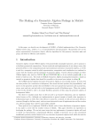
For example, let us draw some vectors, and then draw a bivector:
>> clf(); a = 2 e1 + e3, b = e2,
>> c = ori(e1^e2)
You should see in the graphics window something like Figure 2. Perform GAorbiter to appreciate
the spatial relationships better: note that the circle lies in the plane containing both e1 and e2.
The norm of a bivector is the absolute value of the area it represents:
>> norm((e1+e2)^e3)
ans =
1.4142
2.2.3
Trivectors
Taking the outer product of three vectors yields yet another object, which is naturally called
a trivector. It is a directed volume element. In 3-dimensional space, all such elements must
be multiples of the unit directed volume element, which we denote by I3 . (In other words,
algebraically the trivectors of a 3-dimensional vector space form a 1-dimensional linear space
GABLE Version 1.5 (GABLE+)
Figure 2: a = 2 e1 + e3, b = e2, c = e1^e2
with basis I3 .) In an orthonormal basis e1 , e2 , e3 for our Euclidean 3-space, we equate it with
the volume spanned by the ‘right-handed’ frame: I3 ≡ e1 ∧ e2 ∧ e3 . The unit directed volume
I3 is often called the (unit) pseudoscalar of 3-dimensional Euclidean space.
We have implemented I3 as I3. [[ but it gets cleared when they do clf(). ]] Verify
the outcome of the following expressions by hand, to get some dexterity in manipulations with
the wedge product on the basis of its definition:
>>
>>
>>
>>
>>
>>
>>
e1^(e2^e3)
(e1^e2)^e3
e1^e2^e3
e3^e2^e1
e1^(e1+2*e2)^e3
e1^(e1+2*e2)^e1
norm(e1^e2^e3)
Notice that the trivector e3 ∧ e2 ∧ e1 equals −I3 : these vectors in this order form a ‘left-handed’
frame. The terms denoting ‘handedness’ are therefore not explicit conventions anymore, they
have become part of the computational framework of geometric algebra as the signs of trivectors.
The norm of a trivector is absolute value of the volume; if you need a signed scalar denoting the
volume of a trivector T, use T/I3 .
Conceptually, a trivector represents an oriented volume. Graphically, we represent it by a
sphere, which we render transparently such that it won’t hide all objects inside it. The magnitude
of the trivector is represented by the volume of the sphere. To indicate the orientation (use the
ori() function again), we draw line segments emanating from the surface of the sphere; the
orientation is indicated by whether these line segments go into or out of the sphere. Try
>> s1 = green(ori(I3))
>> s2 = red(ori(-0.5*I3))
2.2.4
Quadvectors?
If you try taking some outer products of four or more vectors, you will find that these are
all zero. You may understand why this should be: since only three vectors in 3-space can be
independent, any fourth must be writable as a weighted sum of the other three; and then the
anti-symmetry of the outer product kills any term in the expansion. For instance:
e1 ∧ e2 ∧ e3 ∧ (e1 + e2 )
=
e1 ∧ e2 ∧ e3 ∧ e1 + e1 ∧ e2 ∧ e3 ∧ e2
=
(e1 ∧ e1 ) ∧ e2 ∧ e2 − e1 ∧ (e2 ∧ e2 ) ∧ e3 = 0.
So the highest order object that can exist in a 3-dimensional space is a trivector. But you can
also see that this is not a limitation of geometric algebra in general: if the space had more
dimensions, the outer product would create the appropriate hyper-volumes.
If all we are interested in is planar geometry, then all vectors can be written as the linear
combination of two basis vectors, such as e1 and e2 ; in that case, the highest order object would
9
GABLE Version 1.5 (GABLE+)
10
be a bivector. We would then call I2 ≡ e1 ∧ e2 a pseudoscalar of that 2-dimensional space. In
n-dimensional space, the pseudoscalar is the highest dimensional object in the space. It received
this rather strange name because it is ‘dual’ to a scalar, as we will see in Section 2.4.3.
2.2.5
0-vectors
In the same vein of the interpretation of k-vectors as geometrical k-dimensional subspaces based
in the origin, we can reinterpret the scalars geometrically. Since these are 0-vectors, they should
represent a 0-dimensional subspace at the origin, i.e. geometrically, a scalar is a weighted
point at the origin. This is a fully admissible geometric object, and therefore it should not be
surprising that it is a member of the basis {1, e1 , e2 , e3 , e1 ∧ e2 , e2 ∧ e3 , e3 ∧ e1 , e1 ∧ e2 ∧ e3 } of
the geometric algebra of 3-dimensional space.
2.2.6
Use: parallelness and spanning subspaces
The outer product of two vectors u and v forms a bivector. When you keep u constant but
make v increasingly more parallel to it (by turning it in the (u, v)-plane), you find that the
bivector remains in the same plane, but becomes smaller, for the area spanned by the vectors
decreases. When the vectors are parallel, the bivector is zero; when they move beyond parallel
(v turning to the ‘other side’ of u) the bivector reappears with opposite magnitude. Try this:
>> a = e1
>> b = e2
>> dynamic{c = ori(a ^ b),}
Drag the vectors a and b using the right mouse button, or assign them a different value on the
console, like
>> a = e2 + 0.05 e1
The dynamic{} statement will be re-evaluated every time a, or b change, adapting the bivector
c. The more parallel the vectors are, the smaller the bivector will be.
A bivector may thus be used as a measure of parallelness: in Euclidean space u ∧ v equals
zero if and only if u and v are parallel, i.e., lie on the same 1-dimensional subspace. Note that
this even holds for 1-dimensional space.
When you’re done with the example from above, use cld(); to remove the dynamic{}
statement. Otherwise it will stick around and confuse you later on.
Similarly, a trivector is zero if and only if the three vectors that compose it lie in the same
plane (2-dimensional subspace). We then do not call them ‘parallel’; the customary expression
is ‘linearly dependent’, but the geometric intuition is the same. If the vectors are ‘almost’ in the
same plane, they span a ‘small’ trivector (relative to their norms times the unit pseudoscalar).
In fact, we can use a bivector B to represent a plane through the origin:
vector x in plane of B
⇐⇒
x ∧ B = 0.
And this B even represents a directed plane, for we can say that a point y is at the ‘positive
side’ of the plane if y ∧ B is a positive volume, i.e., a positive multiple of the unit pseudoscalar
I3 . We will come back to this powerful way of representing planes later (Section 3.7); but for
now you understand why we like to think of a bivector as a directed plane element.
2.2.7
Blades and grades
We now have all the basic elements for our geometric algebra of 3-space: scalars, vectors,
bivectors, and trivectors (pseudoscalars). We have constructed each of these from vectors and
scalars using the outer product. There are some useful terms to describe this construction.
A blade is an object that can be written as the outer product of vectors. For instance, e1 ,
or e1 ∧ (e1 + 2e2 ), or I3 ≡ e1 ∧ e2 ∧ e3 .
The grade of a blade is the dimension of the subspace that the blade represents. So for
instance grade(e1 ∧ (e1 + e2 + e3 )) = 2, and grade(I3 ) = 3. As you see, the outer product of a
object with a vector raises the grade of the object by one (or gives 0).
We can make general objects in our algebra by taking scalar-weighted sums of blades such
as 1 + e1 + e2 ∧ e3 . Such objects are called multi-vectors. In this construction, a blade is called
an m-vector, with m the grade of the blade. In that sense, a scalar is a 0-vector. Often such a
multivector is of mixed grade (do not worry about its geometrical interpretation yet).
GABLE Version 1.5 (GABLE+)
In GAViewer, we have a routine grade that when given an object, returns the grade of that
object. If the object is of mixed grade, grade returns -1. When invoked with a geometric object
and an integer, grade returns the portion of the geometric object of that grade. For example,
>> grade(e1+I3,1)
ans = 1.00*e1
>> grade(e1+I3,3)
ans = 1.00*e1^e2^e3
To test if an object is of a particular grade, use the isGrade command:
>> isGrade(e1^e2,1)
ans = 0
>> isGrade(e1^e2,2)
ans = 1.0
In this context of blades and grades, there is a peculiarity of 3-dimensional space that does
not carry over to higher dimensions: in 3-space (or 2-space, or 1-space), any multivector that is
not of mixed grade can be factored into a blade. For example, we can rewrite e1 ∧ e2 + e2 ∧ e3
as (e1 − e3 ) ∧ e2 . The former is the sum of two bivectors (and thus not in blade form), while the
latter is the outer product of two vectors (and is therefore obviously a blade). In 4-dimensional
space, this fails: e1 ∧ e2 + e3 ∧ e4 cannot be rewritten as the outer product of two vectors.
2.2.8
Other ways of visualizing the outer product
The interpretation of the bivector as a directed circle, which we have used so far, is not what
everyone uses to visualize them. The standard interpretation works directly with the outer
product. If you have e1 ∧ (e1 + e2 ), then for the standard interpretation, we construct the
parallelogram having e1 and e1 + e2 as two of its sides. Graphically, we would draw the vector
(e1 + e2 ) starting from the head of e1 . The area of this parallelogram is the area of the bivector,
and the two vectors give the orientation.
You can see this interpretation of the bivector in GABLE+ using by typing
>> a = factored_bivector(e1, e1 + e2)
Note, however, that the particular vectors used to construct the bivector are not unique. Any
two vectors in this plane that form a parallelogram of the same directed area give the same
bivector. For example,
>> //...
>> b = red(factored_bivector(e1, e2))
will draw a second red parallelogram (a square) that overlaps the first parallelogram. Although
these are two different parallelograms, they are coplanar and have the same directed area,
therefore they represent the same bivector. (If you are having trouble seeing any of the two
bivectors, slide down the alpha value (in the object controls window) for both of them.)
Using GAViewer, you can test that these represent the same bivector by using the equality
operator:
>> e1^(e1+e2) == e1^e2
ans = 1.00
In GAViewer, a result of ‘1’ for a Boolean test means “true” and a result of ‘0’ means “false.”
In our example, this means the geometric objects are the same, which we can also prove algebraically:
e1 ∧ (e1 + e2 ) = e1 ∧ e1 + e1 ∧ e2 = e1 ∧ e2
Note that the area is oriented. In particular, if we reverse the order of the vectors in the
outer product, we get a different result:
>> e1^e2 == e2^e1
ans = 0
However, they only differ by a sign:
>> e1^e2 == -e2^e1
ans = 1.00
11
GABLE Version 1.5 (GABLE+)
This is a result of the bivector representing a directed area: if we reverse the order of the
arguments, then we get the opposite direction.
More generally, we can think of the bivector as representing any directed area within some
simple, closed, directed curve. (To prove this we would need to develop a calculus; we will
not do so in this introduction, so please just accept this statement.) We used a circle for our
representation since we often will not have the creating vectors for a bivector. Indeed, depending
on how we constructed the bivector such vectors may not exist, for example when we take the
dual (Section 2.4.3) of a vector. While we may use any closed curve of the appropriate area,
the circle is the closed curve with perfect symmetry. In our rendering of the bivector, the area
of the circle indicates the area of the bivector; to indicate the orientation of the area, we draw
arrows along its rim.
In a similar manner, we can view a trivector as a parallelepiped. Clear the screen, then run
>> t = factored_trivector(e1,e1+e2,e3)
>> GAorbiter();
to see the parallelepiped constructed for a trivector.
2.2.9
Summary
In this section we have seen the outer product, which combines elements of geometric algebra to
form higher dimensional elements. In particular, the outer product of two vectors is a directed
area element that spans the space containing those two vectors. When applied to other blades
of our space, we get higher dimensional directed volume elements.
If the vectors we combine with the outer product are linearly dependent, then the result of
the outer product will be zero; if they are ‘almost linearly dependent’ in the sense of almost
aligned, the outer product will be small. Therefore the outer product provides a quantitative
and computational way to treat linear dependence.
Exercises
1. Draw the following bivectors e1 ∧ e2 , e2 ∧ e3 , and e3 ∧ e1 , each in a different color. Use
function like red(), white() and blue() to set the color.
2. Redraw the bivectors of the previous exercise using factored bivector(). Based on this
and the previous exercise, do you have a feeling that these bivectors are orthogonal?
3. Draw using factored bivector() the bivectors e1 ∧ e2 and e1 ∧ (e2 + 3e1 ). From this
picture, do you get a feeling whether or not these two bivectors are equal? Test their
equality by comparing them with the == operator.
4. Draw the bivectors e1 ∧ e2 and e2 ∧ e1 . Use the ori() function to draw the orientation
of the bivectors. Are these two bivectors the same? Hint: Notice how the arrows point
in opposite directions. Repeat this exercise using factored bivector() and comment on
the results.
5. Draw the trivector e1 ∧ e2 ∧ e3 the ordinary way (use the ori() function to draw the orientation), and using factored trivector(). Now clear the screen and draw the trivector
e1 ∧ e3 ∧ e2 with both drawing routines. Which graphical representation gives you a better
feel for orientation?
6. Draw the vectors e1 , e2 , and e3 . Next draw the bivector e1 ∧e2 and the trivector e1 ∧e2 ∧e3 .
From this picture, is it easy to tell that the drawn vectors were used to create the bivector
and trivector? Redo this exercise using factored bivector() and factored trivector().
Which graphical representation gives you a better feel for the bivector/trivector that gets
created from particular vectors?
2.3
2.3.1
The inner product
Definition
In a Euclidean vector space, you may have used an inner product, often called the dot product,
to quantify lengths and angles. Geometric algebra also has an inner product, and in our specific
geometric algebra, C3,0 , the inner product on two vectors is the same as the Euclidean inner
product of two vectors.
On vectors, the inner product of our geometric algebra has the standard properties of symmetry and linearity:
12
GABLE Version 1.5 (GABLE+)
13
• u·v =v·u
• (αu + βv) · w = α(u · w) + β(v · w), for α, β scalars
• In Euclidean spaces: u · u > 0 if u is not zero, and u · u = 0 if and only if u is zero
In geometric algebra, the inner product can be applied to any elements of the geometry. Its
definition for such arbitrary elements is rather complicated (for instance, it is neither associative
nor symmetric, though it is linear), and we defer its definition to Section 2.5, although we will
use it before then in some examples to develop a feeling for its meaning.
In our mathematical formulas, we will use ‘·’ to represent the inner product. In GAViewer
we use the . operator:
>> (2 e1 + 3 e3) . e1
ans = 2.00
The inner product takes precendence over the geometric product and addition, so leaving out
the paratheses will give a different result:
>> 2 e1 + 3 e3 . e1
ans = 2.00*e1
// this is equal to 2 e1 + (3 e3 . e1)
The inner product is also defined between a scalar α and a vector u, in which case it is
defined to by their product: α · u = αu; however, the converse is zero: u · α = 0.2 You can also
use it on bivectors and trivectors. Try some:
>>
>>
>>
>>
>>
2 . e1
e1 . 2
e1 . e1^e2 // this is equal to e1 . (e1^e2)
e1^e2 . e1^e2
e1^e2 . -I3
We need to interpret these intriguing results geometrically, and see how we can put this extended
inner product to practical use.
2.3.2
Interpretation: perpendicularity
For two vectors u and v, the inner product u · v is a scalar. From linear algebra, we know how
to interpret this scalar: if two vectors are of unit length, then the inner product is the length of
the perpendicular projection of each vector on to the other, which is equal to the cosine of the
angle between the two vectors. If either vector is not of unit length, then the cosine is scaled
by the lengths of the vectors. So if the angle between vectors u and v is φ, then
u · v = |u| |v| cos(φ).
Thus the inner product is a measure of perpendicularity: if we keep u constant and turn v to
become more and more perpendicular to u, the inner product gets smaller, becomes zero when
they are precisely perpendicular, and changes sign as v moves ‘beyond’ perpendicular.
The inner product keeps this interpretation of perpendicularity when applied to bivectors,
but becomes much more specific geometrically: for instance
x · B is a vector in the B-plane perpendicular to x.
Let us visualize this:
>>
>>
>>
>>
clf();
B = e1^e2
x = yellow(e1+e3) // draw x in yellow
dynamic{ xiB = x . B, }
Because we have made xiB dynamic, it will be recomputed when you can modify B or x. For
¯
instance, use ctrl-right mouse button-drag to move the yellow vector x and see what happens.
When you’re done with this example, use cld(); to remove the dynamic{} statement.
Note that the result is also perpendicular to x and in the B-plane if the vector x was in the
B-plane to begin with.
2 The reader who knows geometric algebra can see that we deviate from the commonly used inner product of
Hestenes here. We will get back to that.
GABLE Version 1.5 (GABLE+)
>>
>>
>>
>>
14
clf();
B = e1^e2
b = yellow(e1)
biB = b . B
So in a sense, the operation ‘·B’, applied to a vector b in the B-plane (so that b ∧ B = 0),
produces the perpendicular to b in that plane, the complement to b in the B-plane. This
generalizes, as we will see later (Section 4.2).
Even with a trivector, the interpretation of the inner product as producing a perpendicular
result remains:
>>
>>
>>
>>
clf();
x = e1+e3
xiI3 = x . I3
GAorbiter();
The inner product x · I3 is now the bivector representing the plane perpendicular to x. Conversely, the inner product of a bivector with a trivector produces a vector perpendicular to the
plane of the bivector:
>>
>>
>>
>>
clf();
B = (e1 + e2) ^ e3
BiI3 = B . I3
GAorbiter();
You begin to see how conveniently the inner and outer product work together to produce simple
expressions for such constructions.
In general, for blades of different grades, if the grade of the first argument is less than the
grade of the second argument, then their inner product is a blade whose grade is the difference in
grades of the two objects, lies in the subspace of the object of higher grade, and is perpendicular
to the object of lower grade. The inner product is thus grade decreasing. However, if the first
argument has a larger grade than the second, our inner product is zero (because of this gradereducing property it is also known as a contraction, and you cannot contract something bigger
onto something smaller).3
But what happens if we take the inner product of two blades of the same grade? We already
know that the inner product of two vectors yields a scalar. Try taking the inner product of two
bivectors:
>> e1^e2 . e2^e3
>> e1^e2 . e1^e2
In both cases, the result is a scalar; in the first example, the result is 0, while in the second
example, it is −1. Likewise, if we take the inner product of the pseudoscalar with itself the
result is a scalar. In general, the inner product of two blades of the same grade results in a
scalar.
2.3.3
Summary
The inner product is a generalization of the dot product, and may be applied to any two elements
of our space. When applied to vectors, it is the familiar dot product. More generally, the inner
product is associated with perpendicularity.
2.4
2.4.1
The geometric product
Definition
We have seen how the inner and outer product of two vectors specify aspects of their perpendicularity and parallelness, but neither gives the complete relationship between the two vectors.
So it makes sense to combine the two products in a new product. This is the geometric product,
and it is amazingly powerful.
We denote the geometric product of objects by writing them next to each other leaving the
multiplication symbol understood. For vectors u and v, we define:
u v = u ∧ v + u · v.
(1)
3 You should be aware that the more commonly used ‘Hestenes inner product’ is not a contraction. More about
this later.
GABLE Version 1.5 (GABLE+)
15
This is therefore an object of mixed grade: it has a scalar part u · v and a bivector part u ∧ v.
This mixed grade is not a problem, as geometric algebra spans a linear space in which such
scalar-weighted combinations of blades are perfectly permissible.
Changing the order of u and v gives:
v u = v ∧ u + u · v = −u ∧ v + u · v,
so the geometric product is neither fully symmetric, nor fully anti-symmetric.
With the geometric product defined, we can use it as the basis of geometric algebra, and
view the inner and outer products as secondary, derived constructions. For instance, for vectors
we we can retrieve the inner and outer products as its symmetric and anti-symmetric parts,
respectively:
u·v
=
u∧v
=
1
(uv
2
1
(uv
2
+ vu)
(2)
− vu)
(3)
and these formulas can be extended to arbitrary multivectors (see Section 2.5). Although the
products algebraically have this relationship to each other (with the geometric product being
the more fundamental one), yet we will show that geometrically it is convenient to think of them
as three basic products, each with their own geometric annotations and usage. Inner product
and outer product are indeed highly meaningful ‘macros’ for geometric algebra.
In GAViewer, you can use the * operator for the geometric product, but you can also omit
it and simply use a space ’ ’ for the geometric product. In this text we will omit the *. Use
the following examples to play around with geometric product a bit– but check the outcomes
by hand to familiarize yourself with the computations.
>>
>>
>>
>>
>>
e1 (e1 + e2) // this is equal to e1 * (e1 + e2)
(e1 + e2)(e1 + e3)
(e1 + e2)(e1 + e2)
e1 e2
e1 e1
The geometric product is extended by linearity and associativity to general multivectors (Section 2.5), which is how we have implemented it. A geometric product of general multivectors
may produce multivector with many different grades:
>> (1 + e1)(e1 e2 + e1^e2^e3 + e1.e2^e3)
ans = 1.00*e2 + 1.00*e2^e3 + 1.00*e1^e2 + 1.00*e1^e2^e3
Here GAViewer may complain that the multivector has no interpretation. You can still use it
in computation, but GAViewer can not draw it.
The geometric interpretation of the geometric product is more difficult than the geometric
interpretations of vectors, bivectors, and trivectors. By Equation 1,
>> e1 (e1 + 2 e2)
results in the scalar e1 · (e1 + 2e2 ) = e1 · e1 = 1 and a bivector e1 ∧ (e1 + 2e2 ) = 2e1 ∧ e2 and
it is hard to understand what that means. We will soon recognize that the geometric product
produces a geometric operator rather than a geometric object, and that therefore we had better
visualize it through its effect on objects, rather than by itself. GAViewer draws the multivector
kind of like a bivector with a arrow in it, which suggests that it has something to do with
rotation.
2.4.2
Invertibility of the geometric product
The inner product and outer product each specify the relationships between vectors incompletely,
so they can not be inverted (e.g., knowing the value of the inner product of an unknown vector x
with a known vector u does not tell you what x is). However, the geometric product is invertible.
This is extremely powerful in computations.
Still, not all multivectors have inverses in general geometric algebras. Fortunately, in the
geometric algebra of Euclidean space, subspaces (represented as blades, i.e., multivectors of a
single grade) do. Thus, for each blade A = 0 in Euclidean space, we can find A−1 such that
AA−1 = 1.
Let us first take a linear subspace, characterized by a vector v. (Why does a vector characterize a linear subspace? Because x ∧ v = 0 characterizes all vectors x in this subspace.) What
is its inverse? Think about this, then ask GAViewer:
GABLE Version 1.5 (GABLE+)
>>
>>
>>
>>
16
v = 2 e1
iv = inverse(v)
v iv
iv v
So, as you thought, the inverse of a vector is parallel to the vector, but differs by a scalar factor:
v−1 =
v
.
v·v
This is easily verified:
v(v/(v · v)) = (vv)/(v · v) = (v · v + v ∧ v)/(v · v) = (v · v + 0)/(v · v) = 1.
Now consider a two-dimensional subspace, characterized by a bivector B. For instance, what
is the inverse of 2e1 ∧ e2 , where the basis {e1 , e2 , e3 } is orthonormal? In such a basis we have:
e1 e1 = e1 · e1 = 1, etc.
and e1 e2 = e1 ∧ e2 , etc.
(4)
With this, we observe that
(e1 ∧ e2 ) (e1 ∧ e2 ) = (e1 e2 )(e1 e2 ) = e1 (e2 e1 )e2 = −(e1 e1 )(e2 e2 ) = −1,
(5)
so, in the sense of the geometric product: the square of a bivector is negative. Then the inverse
is simple to determine: (2e1 ∧ e2 )−1 = − 12 (e1 ∧ e2 ) = 12 e2 ∧ e1 . In general, in C3,0
B−1 =
B
.
B·B
The inverse of a pseudoscalar αI3 is also easy. Observe that
I3 I3
=
(e1 ∧ e2 ∧ e3 )(e1 ∧ e2 ∧ e3 )
=
e1 e2 e3 e1 e2 e3 = −e2 e1 e3 e1 e2 e3
=
e2 e3 e1 e1 e2 e3 = e2 e3 e2 e3
=
−e3 e2 e2 e3 = −e3 e3 = −1
Thus, in our algebra the inverse of αI3 is:
(αI3 )−1 = −I3 /α.
In GAViewer, use inverse() to compute the inverse of a geometric object. As a shorthand for B*inverse(A), you may write B/A. Note that the geometric product is not in general
commutative, so we would write inverse(A)*B as (1/A)*B, which is rarely equal to B/A.
2.4.3
Duality
The dual of an element A of our geometric algebra is defined to be
dualA ≡ A/I3 = −AI3 ,
(6)
and in GAViewer the function dual() returns the dual of an object. The dual of a blade
representing a subspace is a blade representing the orthogonal complement of that subspace,
i.e., the space of all vectors perpendicular to it. This is a common construction, and it is great
to have it in such a simple form: just divide by I3 .
For example, type the following:
>> clf();
>> a = e1
>> b = dual(e1)
The red vector represents e1; the blue circle represents the dual of e1, which is -e2^e3 as shown
by the following derivation:
dual(e1 )
=
−1
e1 I−1
3 = e1 (e1 ∧ e2 ∧ e3 )
=
e1 (e1 e2 e3 )−1 = −e1 e1 e2 e3
=
−e2 e3 = −e2 ∧ e3
GABLE Version 1.5 (GABLE+)
17
The construction is more striking for more arbitrary vectors, of course (see exercises).
Note that for a blade U we have grade (dual(U)) = 3 − grade (U), so that the dual of a
scalar is a pseudoscalar and vice versa: dual(1) = −I3 and dual(I3 ) = 1 (this is true in any
space and partly explains the name ‘pseudoscalar’ for the n-dimensional volume element).
As a consequence of this rule on grades, the dual relationship between vectors and bivectors
is only valid in 3-dimensional space. In 3-space, we may characterize a plane (which is really
a bivector) dually by a vector; that vector is commonly called the normal vector of the plane.
We now see that it is the dual of the bivector. Indeed, both of the following two equations
characterize the same plane B:
x ∧ B = 0 and x · dual(B) = 0.
We recognize the latter as the ‘normal equation’ of the plane B, the inner product of a vector
x with the normal vector n ≡ dual(B) = B/I3 .
This is an example of a duality relationship between the outer product and inner product.
Since the outer product produces an element of geometric algebra, we can take its dual. One
can then prove (nice exercise, try it for vectors)
dual(u ∧ v) = u · dual(v)
and
dual(u · v) = u ∧ dual(v)
(7)
for any multivectors u and v from the geometric algebra of the space with the pseudoscalar I3
used to define the dual.
This is a good moment to explain how the 3-dimensional cross product of vectors fits into
geometric algebra. The cross product obeys
u × v = dual(u ∧ v).
You can see this with the following GABLE+ commands:
>>
>>
>>
>>
>>
>>
clf();
a = e1 + 0.5 e2
b = e1 + e2 + e3
B = a ^ b
d = green(dual(B))
GAorbiter();
Here we see that the red vector is perpendicular to both of the blue vectors. To check that the
dual matches the cross-product, print the dual of B compare it with you own computation of
the cross product.
So we could define the cross product using the above equation. However, we will not do so,
for two reasons. Firstly, the cross product is too particular for 3-dimensional space; in no other
space is the dual of a ‘span of vectors’ a vector of that space. And secondly, its only use is
to characterize planes and rotations. Geometric algebra offers a much more convenient way to
characterize those, directly through bivectors. We have seen this for planes and we will see it
for rotations soon. Since these bivector characterizations are valid in arbitrary dimensions, we
prefer them to any specific, 3D-only construction. So: we will not need the cross product.
Exercises
1. Determine the subspace perpendicular to the vector e1 + 0.2 e3 .
2. Determine the subspace perpendicular to the plane spanned by the vectors e1 + 0.3 e3 and
e2 + 0.5 e3 , in one line of GAViewer.
3. Prove Equation 7.
4. We used the geometric product to define the dual. We can also make the dual using the inner product (thus directly conveying the intuition of ‘orthogonal complement’). Give such
a formulation of the dual in a way that is equivalent to the geometric product formulation
of the dual and show this equivalence.
2.4.4
Summary
The geometric product is a third product of our geometric algebra. Unlike the inner and outer
products, the geometric product is invertible, which is useful when doing algebraic manipulations. In Section 3, we will see geometric interpretations of the geometric product.
GABLE Version 1.5 (GABLE+)
2.5
18
Extension of the products to general multivectors
We have stated that the inner, outer, and geometric products can be generalized to arbitrary
multivectors. In this section, we will first show how to extend the definition of the geometric
product to general multivectors. Once we have that, it is easy to extend the inner and outer
products.
For general objects of geometric algebra, the geometric product can be defined as follows
(this is not the only way, but it is the most easy to understand). In the n-dimensional vector
space considered, introduce an orthogonal basis {e1 , e2 , · · · , en }. Use the outer product to
extend this to a basis for the whole geometric algebra (the one containing e1 ∧ e2 , etcetera).
Any multivector can be written as a weighted sum of basis elements on this extended basis.
The geometric product is defined to be linear and associative in its arguments, and distributive
over +, so it is sufficient to defined what the result is of combining two arbitrary elements of
the extended basis. We first observe that the desired compatibility with Equation 1 combined
with the orthogonality of the basis vectors leads to
ei ej = −ej ei
if i = j
(8)
because on the orthogonal basis, effectively ei ej equals ei ∧ ej if i = j. If i = j, Equation 1
gives the scalar result ei · ei , which in our Euclidean space equals 1.4 So we have
ei ei = 1.
(9)
This is now enough to define the geometric product of any elements in the geometric algebra.
For instance (2 + e1 ∧ e2 )(e1 + e2 ∧ e3 ) is expanded by distributivity over + to 2e1 + (e1 ∧ e2 )e1 +
2(e2 ∧ e3 ) + (e1 ∧ e2 )(e2 ∧ e3 ). The term (e1 ∧ e2 )e1 in this equals (e1 e2 )e1 , and by associativity
this equals e1 e2 e1 . We apply Equation 8 to get −e1 e1 e2 , and then Equation 9 to get −e2 .
The other terms are computed in a similar way. Note that this definition is heavily based on
the introduction of an orthogonal basis (which is somewhat inelegant); other definitions manage
to avoid that. You may also think that all these expansions make the geometric product an
expensive operation. But the above was just to show how those minimal definitions actually
define the outcome mathematically; a more practical computation scheme using matrices on
the extended basis is what we used to make the orginal GABLE (such details may be found in
[14, 15]).
Now that we have defined the general geometric product, it is easy to generalize both the
inner and outer products. Both products are linear in their arguments, and so are sufficiently
specified when we say what they do on blades. For instance, if we would want to know the
outcome of (A1 + A2 ) · (B1 + B2 ) (where the index denotes the grade of the blades involved),
then this can be written out as A1 · B1 + A1 · B2 + A2 · B1 + A2 · B2 .
For a blade U of grade r, and a blade V of grade s, the definitions for inner and outer
products are:
U · V = grade(UV, s − r)
U ∧ V = grade(UV, s + r).
Since no element of geometric algebra has a negative grade, the inner product is only non-zero
if s ≥ r.5 Note that the inner product lowers the grade, and the outer product increases the
grade.
For a vector u and an s-blade V, these formulas can be shown to produce:
u∧V
u·V
=
1
(uV
2
=
1
(uV
2
+ Vu)
(10)
− Vu).
(11)
as a shorthand for (−1)s V (it is sometimes called the grade involution).
where we used V
Compare this to equations (3) and (2).
Beware: it is not generally true that UV = U · V + U ∧ V; that is only so if U is a vector.
For instance, compute the geometric product of two specific bivectors:
4 To get a general geometric algebra, of a space with a quadratic form (‘metric’) Q, this is set to some specified
scalar Q(ei ), usually taken to be +1 or −1. The sign of Q(ei ) is called the signature of ei .
5 In this the inner product we use as a default in the GABLE+ tutorial deviates from the most commonly used
inner product in geometric algebra, as defined by Hestenes, which has |s − r| rather than (s − r). Our product has a
more direct geometric interpretation, which we will need in the later chapters.
GABLE Version 1.5 (GABLE+)
19
>> (e1^e2)*((e1+e2)^e3)
ans =
-1*e2^e3 + -1*e3^e1
>> inner((e1^e2),((e1+e2)^e3))
ans =
0
>> (e1^e2)^((e1+e2)^e3)
ans =
0
In general, the geometric product of an r-vector and an s-vector contains vectors of grade
|r − s|, |r − s| + 2, · · · r + s − 2, r + s; the inner and outer product specify only two terms of
this sequence, and are therefore only a partial representation of the geometric product (which
contains all geometric relationships between its arguments). For objects other than vectors,
there is much more to geometric algebra than just perpendicularity (inner product) and spanning
(outer product), but in this tutorial we focus on those.
There are some useful formulas permitting the computation of the inner product of multivectors made using the geometric product or the outer product. We state them without proof,
for vectors u and pure blades U, V and W (the general case then follows by linearity).
3
· W)
u · (VW) = (u · V)W + V(u
(12)
∧ (u · W)
u · (V ∧ W) = (u · V) ∧ W + V
(13)
(U ∧ V) · W = U · (V · W)
(14)
Geometry
In this section we will show how the products of geometric algebra can be used to perform many
geometrical tasks.
3.1
Projection, rejection
Given a subspace and a vector, one operation we commonly need to perform is to find the part
of the vector that lies in the subspace and the part of the vector that lies outside the subspace.
These operations are called projection and rejection respectively. Both are easy to perform with
geometric algebra.
Let us begin with a vector v and the desire to write it as v⊥ + v relative to a subspace
characterized by a blade M, where v⊥ is the component of v perpendicular to M, and v the
parallel component. Therefore v⊥ and v need to satisfy
v⊥ · M = 0 and v ∧ M = 0.
Thus
v⊥ M
=
v⊥ · M + v⊥ ∧ M
=
v⊥ ∧ M
=
v⊥ ∧ M + v ∧ M
=
v ∧ M.
But we can divide by the blade M, on both sides, so we obtain:
v⊥ = (v ∧ M)/M
(15)
v = (v · M)/M.
(16)
A similar derivation shows that
These are the general projection and rejection formulas for a vector v relative to any subspace
with invertible blade M, in any number of dimensions. Powerful stuff!
It is important to visualize what is going on. Take M to be a 2-blade, determining a plane.
Then v ∧ M is a volume spanned by v with that plane. It is a ‘reshapable’ volume: any vector v
that has its endpoint on the plane parallel to M, through v’s endpoint, spans the same trivector.
The division by M in the formula for the projection demands the factoring of this volume into
a component M, and therefore returns what is left: the unique vector perpendicular to M that
spans the volume. This is a general property:
GABLE Version 1.5 (GABLE+)
20
Dividing a space B by a subspace A produces the orthogonal complement to A in B.
If A is not a proper subspace, other things happen that we’ll cover later.
These relationships can be seen in GAViewer. To begin, clear the graphics screen (clf())
and draw a bivector. For this demonstration, we will use factored bivector() to draw the
graphical representation of a bivector. Next, draw a vector that lies outside the plane of this
bivector:
>> clf();
>> B = factored_bivector(e1,e1+e2)
>> v = 1.5 e1 + e2 / 3 + e3
To get a better feel for the 3D relationships, use the mouse or GAorbiter() to rotate around
the scene a bit.
We can now type our formulas for the perpendicular and parallel parts of v directly into
GAViewer and draw the resulting perpendicular and parallel components of v relative to B:
>> //... needs v,B
>> vpar = green(v.B / B)
>> vperp = magenta(v^B / B)
We stated that this computation works for any subspace B. In particular, we can set B to be a
vector, and the same computations for vpar and vperp work. Try this!
As we will see later (but you could try it now), you may project a bivector A onto a bivector
B using the ‘same’ formula: A = (A · B)/B. However, the rejection of the bivector is now not
obtained by A⊥ = (A ∧ B)/B, (which is zero since quadvectors do not exist in 3D), but simply
by A⊥ = A − A (a formula that also works in the previous case where A is a vector). More
about the relationships of subspaces in Section 4.
Exercises
1. Redo the example of projection and rejection using the same v as above, but with B=e1+e2.
2. Let v = −3e1 − 2e2 and let B = 2e2 ∧ (e3 + 3e1 ). Compute the projection and rejection
of v by B. Draw v, B, and this projection and rejection. Try this exercise once using
factored bivector() to draw B and a second time using draw to draw B.
3. With the same v and B as the previous exercise, study how the rejection formula works:
first draw v ∧ B using factored trivector(); as decomposition use v, v · B and the
projection P( (v), B). Then draw that trivector again in a decomposition that uses the
rejection.
4. Prove the formula for projection: v = (v · M)/M.
5. (Not easy!) Using Equations 12, 13 and 14, show that
((a ∧ b) · M)/M = a ∧ b
(still a useful exercise!). This gives two ways to compute the projection of a bivector a ∧ b
relative to a blade M. Which do you prefer and why?
3.2
Orthogonalization
Geometric algebra does not require the representation of its elements in terms of a particular
basis of vectors. Therefore the specific treatment of issues like orthogonalization are much less
necessary. Yet it is sometimes convenient to have an orthogonal basis, and they are simple to
construct using our products.
Suppose we have a set of three vectors u, v, w, and would like to form them into an
orthogonal basis. We arbitrarily keep u as one of the vectors of the perpendicularized frame,
which will have vectors denoted by primes:
u ≡ u.
Then we form the rejection of v by u , which is perpendicular to u :
v ≡ (v ∧ u )/u
GABLE Version 1.5 (GABLE+)
21
Now we take the rejection of w by u ∧ v , which is perpendicular to both u and v :
w ≡ (w ∧ u ∧ v )/(u ∧ v )
and we are done. (This is the Gram-Schmidt orthogonalization procedure, rewritten in geometric
algebra.) Here’s an example (no need to type it, use GAblock1();, see section 1.2):
>> // GAblock1();
>> // ORTHOGONALIZATION
>> clf();
>>
>>
>>
>>
// the original vectors
u = green( e1+e2 ),
v = green( 0.3*e1 + 0.6*e2 - 0.8*e3 ),
w = green( e1 -0.2*e2 + 0.5*e3 ),
>>
>>
>>
>>
// and orthognalized:
u_p = red( u ),
v_p = red( (v^u_p)/u_p ),
w_p = red( (w^u_p^v_p)/(u_p^v_p) ),
>> GAorbiter();
You might want to draw the duals to show the perpendicularity of the resulting basis more
clearly (see Exercise 1).
Note that in this construction, v ∧u = v u = v∧u, and w ∧v ∧u = w (v u ) = w∧v∧u,
so that it preserves the trivector spanned by the basis, in magnitude and orientation. Check
this in GAViewer:
>> (u ^ v ^ w) == (u_p ^ v_p ^ w_p)
ans = 1.00
As an exercise, you might want to give the algorithm for n-dimensional orthogonalization.
Exercises
1. Convince yourself that up, vp and wp are orthogonal, using graphics routines to explore
their construction. You might for instance draw dual(up), and in that plane study vp and
wp.
3.3
Reflection
Suppose we wish to reflect a vector v through some subspace (a vector, a plane, whatever). In
a geometric algebra, this subspace is naturally described by a blade, so we will look at reflecting
v through a unit blade M. If we write v as
v = v⊥ + v ,
where v⊥ is the part of v perpendicular to M and v is the part parallel to M (we derived
formulas for both in the Section 3.1), then r, the reflection of v through M, is given by
r = v − v⊥ .
Using our formulas for the parallel and perpendicular parts of v relative to M, we see that
r
=
v − v⊥
=
(v · M)M−1 − (v ∧ M)M−1
=
1
(vM
2
=
v)M−1 − 12 (vM + −M
Mv)M−1
−
MvM−1 .
This is an interestingly simple expression for such arbitrary reflections.
Let us see what the formula yields for specific choices of the blade we reflect in. In 3D, there
are four possibilities for the blades.
GABLE Version 1.5 (GABLE+)
22
r
m
v
v
v
Figure 3: Reflecting v through m.
• scalar: M = 1
The scalar, viewed as a subspace, is a point at the origin (see Section 2.2.5). And indeed,
our reflection formula yields v → − v, which is clearly a point reflection in the origin.
• vector: M = u
Let the blade M characterize the reflecting subspace be a unit vector u; then the reflection
is relative to a line in direction u. This gives
r = uvu.
An attractive formula for a basic process!
• bivector M = B
For a plane in 3D characterized by a unit bivector B (so that B2 = −1, and therefore
B−1 = −B), we obtain
r = BvB.
We could also write this in terms of the dual to the plane, i.e., the normal vector n defined
as n = BI−1
3 :
r = BvB = nI3 vnI3 = nI23 vn = −nvn.
(It is a good exercise to prove r = −nvn for reflection in a hyperplane dual to n in
arbitrary-dimensional space.)
You can see this in GAViewer with the following sequence of commands:
>>
>>
>>
>>
clf();
v = yellow(e1 + 2 e3)
M = e1 ^ e2
v_r = M v M
• volume M = I3
Since I3 = −I3 and I3 commutes with v, this gives v → v. Reflection in the containing
space is the identity, since v⊥ = 0.
To develop the formula for the reflection of an arbitrary blade of grade k in the blade M of
grade m, first see what happens for the geometric product of the reflection of k vectors:
(−
Mu1 M−1 )(−
Mu2 M−1 ) · · · (−
Muk M−1 ) =
=
u1 M−1 M
u2 M−1 · · · M
um M−1
(−1)k M
=
(−1)k+km Mu1 M−1 Mu2 M−1 · · · Muk M−1
=
(−1)k(m+1) Mu1 u2 · · · uk M−1 .
Therefore:
X even grade :
X odd grade :
X → MXM−1
X → −
MXM−1
A bit complicated; but that is how reflections are for such subspaces.
By the way, you see from this what happens if you reflect a plane characterized by a bivector B, relative to the origin: it is preserved. However, its normal would reflect, and that is
undesirable. In the past, when people could only characterize planes by normal vectors, they
GABLE Version 1.5 (GABLE+)
23
therefore had to make two kinds of vectors: position vectors which do reflect in the origin, and
‘axial’ vectors which don’t, and realize that a normal vector is an axial vector. Using bivectors
directly to characterize planes, we have no need of such a strange distinction: the algebra and
its semantics simplifies by admitting objects of higher grade!
Exercises
1. Reflect the bivector B = (e1^e2 + 2/3 e2^e3 + e3^e1/3) through the plane spanned by
the bivector M = e1^e2. Note carefully what happens to the orientation of the bivector.
Is that what you expected?
2. Reflect the pseudoscalar I3 through a bivector. Note the orientation.
3. Do orientation and magnitude of the reflecting blade M matter to the reflection result?
3.4
Rotations
3.4.1
Rotations in a plane
Consider a vector a, and a vector b that is ‘a rotated version of a’. We can try to construct b
as the multiplication of a with some element R of our algebra:
b = Ra,
and since the geometric product with a is invertible we find simply that
R = b/a =
ba
.
a·a
This is a bit too general to describe a rotation, since we have nowhere demanded explicitly that
a and b should have the same norm. Therefore ba contains both a rotation and a dilation
(‘stretch’) of the vector a. This is then a possible interpretation for the geometric product: ba
is the operator that maps a−1 to b. (Or, alternatively, b/a is the operator that transforms a
into b.)
For the pure rotation we wished to consider, the length of the rotated vector (and equivalently, the norm of the vector) does not change. To create an R that does not depend on the
length of the vectors we used to construct it, we should construct R using vectors of the same
norm in the direction of a and b; for instance, both unit vectors. In Euclidean space the inverse
of a unit vector is the vector itself. So then we get: a rotation operator is the geometric product
of two unit vectors (and vice versa).
Try this in GAViewer using the following sequence of commands:
>>
>>
>>
>>
clf();
a = blue( e1 )
b = blue( unit(e1+e2) )
R = b / a
At this point, we see the vectors a and b drawn in blue and R in red. By construction, they are
separated by a 45 degree angle. If you now type:
>> //... needs a,R
>> b = alpha(blue(b), 0.5), // make ’b’ transparent
>> Ra = R a
we see a red vector drawn over-top b, since this is a rotated to become b. Rotating this vector
a second time and looking from above
>> //... needs a,R
>> RRa = green( R R a )
we see that we have rotated a by the angle between a and b (45 degrees) twice, giving rotation
of a by 90 degrees (drawn in green).
You can use this rotation to rotate any vector in the a ∧ b-plane; for instance, if you wish
to rotate c = 2a + b, then you are looking for a vector d such that d is to c as b is to a. In
formula: d/c = b/a, and therefore d = (b/a)c = Rc. Let us try that:
>> //... needs a,b
>> c = magenta( 2 a + b )
>> Rc = magenta( R c )
GABLE Version 1.5 (GABLE+)
24
Writing things in their components of fixed grade, the expression for R is (taking a and b
unit vectors)
R = ba = b · a + b ∧ a = cos φ − i sin φ,
where i is the bivector denoting the oriented plane containing a and b, oriented from a to b,
and φ is the angle between them in that oriented plane, so from a to b. Note that if we would
orient the plane from b to a, then i would change sign, and R would only be the same if φ
changes sign as well. So the orientation of i specifies how to measure the angle.
If you have had complex numbers or Taylor series in your math courses, you may realize
that we can write the above as an exponential:
cos φ − i sin φ = e−iφ
This is based on i2 = −1, which is correct since i is a unit bivector in C3,0 (Equation 5). If
you have not had those subjects, just consider this as a definition of a convenient shorthand
notation in terms of ‘abstract’ exponentials. In fact, there are several equivalent ways of writing
the relationship between a and b, and hence the rotation over the ‘bivector angle’ iφ:
b = e−iφ a = aeiφ .
The sign-change in the exponent is due to the non-commutative properties of the geometric
product. So i is not really a complex number: then the order would not have mattered.
As we showed before when rotating the vector c = 2a + b, you can use this formula to rotate
arbitrary vectors in the i-plane over an angle φ as
Rx = e−iφ x.
Let us try this, using the geometric exponent function exp():
>>
>>
>>
>>
>>
>>
clf();
i = e1 ^ e2
R = exp(-i pi/2)
a = e1
Ra = green( R a )
aR = yellow( a R )
Note that Ra indeed rotates a over π/2 in the positive orientation direction of the plane e1 ∧ e2
(from e1 to e2 ), and aR is the opposite orientation (it rotates over −π/2). If you print R, you
will notice that there are some numerical issues: it is not the pure bivector it should have been,
but this affects the result R*a but little. Geometric algebra is numerically stable!
However, if x is not in the i-plane, the formula e−iφ x does not produce a pure vector. You
might try this, for instance with b=e1+e3; you will see something a bit surprising. So the above
rotation formulas (Ra and aR) only work for vectors a in the plane in which R is defined; i.e.,
we do not yet have the formula for general rotations in 3-space, which is the topic of the next
section.
3.4.2
Rotations as spinors
There is a better representation of those rotations that keep the i-plane invariant, and which
will work on any vector, whether in the i-plane or not. We construct it by realizing that a
rotation can be made by two reflections. We saw in Section 3.3 that the reflection of a vector x
in a vector a can be written as: axa−1 . Following this by a reflection in a vector b we obtain
(take a and b as unit vectors):
b(axa−1 )b−1 = (ba)x(ba)−1 = e−iφ/2 xeiφ/2 ,
where i is the plane of a and b (so proportional to a ∧ b) and φ/2 the angle between a and
b. This produces a rotation over φ, as you may find by inspecting Figure 4 or writing out the
shorthand explicitly. In doing this, it is convenient to split x in components perpendicular and
contained in i, and to use that x⊥ i = ix⊥ (since x⊥ · i = 0) and x i = −ix (since x ∧ i = 0):
e−iφ/2 xeiφ/2
=
(cos(φ/2) − i sin(φ/2))x(cos(φ/2) + i sin(φ/2))
=
(cos(φ/2) − i sin(φ/2))(x⊥ + x )(cos(φ/2) + i sin(φ/2))
GABLE Version 1.5 (GABLE+)
25
Figure 4: A rotation represented as two reflections.
=
(cos2 (φ/2) − i2 sin2 (φ/2))x⊥ + x (cos2 (φ/2) − sin2 (φ/2) + 2 sin(φ/2) cos(φ/2) i)
=
x⊥ + x (cos(φ) + sin(φ)i)
=
x⊥ + x eiφ
So the perpendicular component is unchanged, and the parallel component rotates over φ.
Therefore the rotation of x over φ in the i-plane is given by the formula
x → e−iφ/2 xeiφ/2 .
This formula represents the desired rotation. Let us try the last example of the previous section
(a 90 degree rotation in the e1 ∧ e2 -plane) again, now properly using the new formula:
>>
>>
>>
>>
>>
>>
>>
clf();
i = e1 ^ e2;
R = exp(-i pi/2/2) // note the half angle!
a = green( e1 )
b = green( e1 + e3 )
Ra = R a / R
Rb = R b / R
The new formula easily extends to arbitrary multivectors, as follows. Suppose we want to rotate
cd. We can perform this rotation by rotating c and d independently and multiplying the results.
But this is simply
−iφ/2 iφ/2 −iφ/2 iφ/2 −iφ/2
e
ce
e
de
= e
cdeiφ/2 .
Linearity of the rotation permits us to rotate sums of geometric products using this formula;
and since that is all that inner products and outer products are (see Equations 10 and 11), the
formula applies to those as well. Therefore, characterizing a rotation R by R = e−iφ/2 , we can
use it as
X → RXR−1
to produce the rotated version of X, whatever X is.
>> //... needs a,b,R
>> aob = a ^ b
>> Raob = R aob / R
The object R = e−iφ/2 is called a spinor (or sometimes a rotor). It is all we need to characterize
a rotation in n dimensions. Composition of rotations (independent of what we are going to
rotate) is then just a multiplication of their spinors. For rotating X first by R1 and then by R2
gives:
R2 (R1 XR1−1 )R2−1 = (R2 R1 )X(R2 R1 )−1
which is a new rotation using the spinor R = R2 R1 . Be careful, though: spinors do not commute,
so you cannot simply say e−i2 φ2 e−i1 φ1 = e−(i2 φ2 +i1 φ1 ) .
GABLE Version 1.5 (GABLE+)
26
Exercises
1. On paper and on the computer, make an operator that implements a rotation of 90 degrees
around the e1 axis, followed by 90 degrees around the e2 axis. After you have constructed
it, write it in exponential form again (on paper only) – this should give you the effective
total rotation, in terms of a rotation plane and an angle.
2. Repeat the same exercise using rotation matrices; especially the final step of retrieving
axis and angle is quite a bit more work!
3. Draw, rotate and draw a bivector, and make sure your intuition keeps up with these results!
4. What happens when you rotate a trivector? Can you prove that?
3.4.3
Rotations around an axis
In the previous section, we took a rotation in the plane and extended it to a rotation in 3-space.
However, we can also characterize rotations in 3-dimensions by an axis and an angle. You may
wonder how this 3-dimensional rotation is related to the above rotation.
The answer: it is simply related by duality. We can rewrite the bivector iφ/2 (the rotation
plane and angle) as
iφ/2 = (iφ/2)I−1
3 I3 = (dual(i)φ/2)I3 = (uφ/2)I3 = I3 uφ/2,
with u ≡ dual(i) the unit vector dual to i. It is the rotation axis. Thus a rotation in 3D may
be characterized by a vector of length φ/2 along the axis u:
R = e−iφ/2 = e−I3 uφ/2
A very handy formula, all you need is uφ to get a computable representation of the rotation! This
is natural, much more so than rotation matrices in which the axis is hidden as the eigenvector
of eigenvalue 1, and the angle in the complex eigenvalues or the trace. (Beware: in higher
dimensions, this rewriting does not work, and you will have to use the bivectors. For instance
in 4-dimensional space the dual of the bivector characterizing the rotation plane is a bivector;
rotations in 4D do not have an axis).
Obviously, all this is similar to the cross product trick, which is also valid in 3D only. We
have seen that a × b = dual(a ∧ b), so that u = dual(i) can be written as the cross product
of two vectors in the i-plane. However, the characterization of rotation by a bivector works in
arbitrary dimensions, and is therefore a good habit even in 3D.
To move back and forth between the spinor in exponential form, and the argument of the
exponential, it is convenient to have an inverse of the exponential, i.e., a logarithm. This inverse
is not unique, since if R = exp(iφ/2), then also exp(iφ/2 + 2πi) = R; so the logarithm of
a spinor has multiple values (those of you familiar with complex analysis may recognize the
phenomenon). In the implementation for the logarithm of a spinor we choose the value of the
bivector between −πi and πi; this is the function sLog(). You see it used in the exercise below.6
Exercises
1. Verify that the following code is an implementation of the first exercise of the previous
section. Note especially how we retrieve the direction of the effective rotation axis.
>>
>>
>>
>>
>>
>>
// GAblock2();
// ROTATION EXERCISE
clf();
R1 = exp(-I3 e1 pi/2/2);
R2 = exp(-I3 e2 pi/2/2);
R = R2 R1
>>
>>
>>
>>
// The objects and the rotor:
a = blue( e1 + e2 )
Ra = magenta( R a / R )
RRa = red( R Ra / R )
6 If you use sLog() on a non-unit spinor S, then there is an additive scalar term equal to log(|S|), in agreement
with the usual behavior of the logarithm on products.
GABLE Version 1.5 (GABLE+)
27
>> // // The axis of rotation:
>> axisR = green( grade(unit(-(sLog(R))/I3 ), 1) )
3.5
Orientations in 3-space
When a vector, bivector, or other geometric element is rotated relative to another element, we
can use that to encode orientation. This representation is itself an element of the geometric
algebra. Here is how that works, in a Euclidean space.
3.5.1
Interpolation of orientations
Interpolation between orientations in 3-space is a notorious problem; often required, but not
easy to do tidily in many a classical representation. In geometric algebra, the problem is fairly
easily solved – about as easily as it is stated. First, we characterize orientations in terms
of rotation operators, in a coordinate-free manner. The idea is straightforward: when you
consider an object to have a certain orientation, what you mean is that relative to its standard
orientation (whatever that may be), it has undergone some rotation R. So its orientation may be
characterized by this rotation R. If we have two orientations, then these may be characterized
by two rotations RA and RB . A smooth interpolation between these two orientations may then
be achieved by n intermediate identical rotation operators R, to be applied to RA , so that the
subsequent rotations are
R0 = RA ;
Ri+1 = R Ri ;
Rn = RB .
The intermediate orientations of whatever object X we wanted oriented are then Ri XRi−1 ,
for i = 1, · · · , n. With this specification of the manner of rotation (n identical operators) the
problem can be solved in a fairly straightforward manner.
The total rotation to be made by the n operators R is the rotation from RA to RB , which
−1
. This should equal Rn , so we have
is RB RA
−1
= e−I3 aφ/2 ,
Rn = RB RA
where a and φ follow from RB and RA (see below for an example). The solution is then
R = e−I3 aφ/2
1/n
= e−I3 aφ/(2n) .
Taking the n-th root of a spinor can be done by taking its logarithm using sLog() (giving the
argument of the exponential), dividing by n, and then exponentiating.
The following example shows the computations to implement this. Let RA be the orientation
achieved from some standard orientation by a rotation over Ie1 π/2, and let RB be the rotation
Ie2 π/2. Let us say that the aim is to get from RA to RB in eight intermediate steps. We
compute:
>>
>>
>>
>>
>>
>>
>>
>>
// GAblock3();
// INTERPOLATION OF ORIENTATIONS
clf();
RA = exp(-::I3 e1 pi/2/2);
RB = exp(-::I3 e2 pi/2/2);
Rtot = RB/RA;
n = 8;
// we rotate in 8 steps
R = exp(sLog(Rtot)/n)
To demonstrate the correctness, we need an object that shows the orientations. So we choose
to draw some bivector u^v in orientation RA and RB, and show the intermediate orientations.
>> //... needs n, R, RA, RB
>> u = e1+e2-e3;
>> v = e1+e3;
>> // === initial orientation:
>> O[0] = blue( factored_bivector(RA u / RA, RA v / RA) )
>> // === final orientation:
GABLE Version 1.5 (GABLE+)
Figure 5: Interpolation of orientations for a bivector.
>> O[n] = green( factored_bivector(RB u / RB, RB v / RB) )
>> axisR = red( grade(unit(-sLog(R)/I3), 1) )
>> Ri = RA;
>> for (i = 1; i < n; i = i + 1) {
Ri = R Ri;
ui = Ri u / Ri;
vi = Ri v / Ri;
O[i] = factored_bivector(ui, vi);
// interpolate the color:
c = get_color(O[0]) * (n - i) / n + get_color(O[n]) * i / n;
O[i] = color(O[i], c),
}
This gives a result similar to Figure 5. Make sure you understand the reason behind these
steps (the drawnow command forces Matlab to display the draw commands in DrawBivector;
without this command, nothing would be displayed until the for loop was exited). If you have
learned about quaternions before, you may realize that the above geometric algebra approach
to interpolating orientation is equivalent to unit quaternions (see also next section). For most
people, those are an isolated technique; you may now appreciate how they are a natural part of
the algebraic structure of the 3-dimensional space.
Exercises
1. Verify the axis and angle in the example above by hand.
2. What happens in the example if one of the rotations, say RB , was over 180 degrees, so
ψ = π. Is the solution still well-behaved?
3. What happens if RA and RB occur in the same plane?
3.6
Complex numbers and quaternions: subsumed
So rotations are characterized by the plane in which they occur; those planes are characterized
by bivectors; and combinations of rotations are represented by geometric products of these
bivectors. If you have heard of complex numbers and quaternions, you know that those may
also be used to do rotations, in the plane and in space, respectively. How does this compare
to the geometric algebra method? Surprisingly, the answer is: it is exactly the same (but in a
richer context)!
Algebraically, we may observe that the linear space C3,0 has several interesting subspaces
with corresponding sub-algebras. In particular, consider the subspace spanned by {1, e1 ∧ e2 }
on an orthonormal basis e1 , e2 , e3 . The product of e1 ∧ e2 with itself is
(e1 ∧ e2 )(e1 ∧ e2 ) = e1 e2 e1 e2 = −e1 e1 e2 e2 = −1.
28
GABLE Version 1.5 (GABLE+)
29
Thus in this subspace, the bivector e1 ∧ e2 has similar properties to the complex number i,
and we see that indeed we can use this linear subspace of our geometric algebra spanned by 1
and e1 ∧ e2 as the complex numbers, with their product represented by the geometric product
(at least if we are careful about the order, due to difference in the commutative properties of
the two algebras). Within geometric algebra, these can be seen as operators, which can act on
geometrical subspaces represented by vectors, bivectors, trivectors or scalars. Complex numbers
can only multiply each other, not ‘operate’ on other objects such as vectors.
Now consider the subalgebra spanned by {1, e1 ∧ e2 , e2 ∧ e3 , e1 ∧ e3 }. The analysis of the
previous paragraph shows that
(e1 ∧ e2 )2 = (e2 ∧ e3 )2 = (e1 ∧ e3 )2 = −1,
Further, we have
(e1 ∧ e2 )(e2 ∧ e3 )
=
e1 ∧ e3
(e2 ∧ e3 )(e1 ∧ e3 )
=
e1 ∧ e2
(e1 ∧ e3 )(e1 ∧ e2 )
=
e2 ∧ e3
and changing the order in which we multiply these bivectors changes the sign of the result. In
other words, with the identification i = e1 ∧ e2 , j = e2 ∧ e3 , and k = e1 ∧ e3 we get:
i2 = j 2 = k2 = −1,
i j = k, j k = i, k i = j.
You may recognize this: they are the defining equations of quaternions, usually introduced as a
special ‘number system’, somehow mysteriously handy for computations with rotations.
Now we see that the basic ‘complex numbers’ occurring in quaternions are actually a basis
of bivectors in the geometric algebra C3,0 . Those seemingly imaginary numbers are actually
real spatial planes in disguise, and their product is just the geometric product. Not a big surprise, then, that quaternions are so useful in describing orientations: quaternions are actually
disguised spinors representing the rotation planes, and their products therefore represent successive rotations. Within the same framework, we can now also represent the objects on which the
rotations need to act, and that is a significant improvement over the quaternion representation.
3.7
3.7.1
Subspaces off the origin
Lines off the origin
You may have noticed that most of the objects we have drawn are based about the origin.
Vectors start from the origin, bivectors and trivectors contain the origin. It is possible, however,
to describe objects that are not centered at the origin, basically by adding a vector, bivector,
etcetera to offset them to where we desire. Let’s see how.
We have already seen that a blade B characterizes a subspace through the outer product,
as follows: the equation
x∧B= 0
holds if and only if x is linearly dependent on the vectors ‘in’ the blade. So in particular, if the
blade is a vector v, the equation x ∧ v = 0 characterizes the vectors of points on the line in
direction v, through the origin. Its parametric solution is x = τ v, for any real number τ .
To characterize a line off the origin, through a point p, we simply translate x, i.e., we let
x − p satisfy the line equation. This gives
x∧v =p∧v
as the implicit equation of the line parallel to v, through p. So all points x on the line span the
same bivector with v. A line is thus implicitly characterized by a vector v (called the tangent)
and a bivector V ≡ p ∧ v (called the moment), and determined by an arbitrary vector p on the
line. These terms are illustrated in Figure 6.
This implicit characterization of the line leads to a parametric specification of the points on
it, which is
x = (p ∧ v)/v + τ v.
GABLE Version 1.5 (GABLE+)
30
tangent
v
p
V/v
V=p^v
moment
perpendicular support vector
Figure 6: A line described by offset p and tangent v, with moment V.
’You may recognize in the first term the rejection of p by v, i.e., the perpendicular support
vector of the line. It can also be written in terms of the moment as V/v. The variable τ is a
real number; as it varies from −∞ to +∞ we obtain all points on the line.
(For those interested, here is how the parametric equation is obtained from the implicit
equation x ∧ v = V. First write it as: xv = V + x · v, then divide out v to obtain: x =
V/v + (x · v)/v = V/v + (x · v−1 )v. Now recognize that x · v−1 is a real number taking values
between −∞ and +∞, effectively specifying for each point x its characterizing parameter; call
it τ , and you have the parametric equation.)
So for example, if we want a line parallel to v = e2 that passes through p = e1 + e2 , we are
interested in all vectors x satisfying the equation x ∧ e2 = (e1 + e2 ) ∧ e2 = e1 ∧ e2 . Obviously
x = e1 + τ e2 is the parametric solution, and this is readily verified:
x ∧ e2 = (e1 + τ e2 ) ∧ e2 = e1 ∧ e2 = (e1 + e2 ) ∧ e2 ,
for all real numbers τ . For example, e1 + 2e2 lies on our line. We can test this in GAViewer by
checking that the equation is satisfied:
>> (e1 + 2 e2) ^ e2 == (e1 + e2) ^ e2
ans = 1.00
We can give a graphic illustration of the bivector equality characterizing a line by using factored bivector().
First draw the defining bivector for the line, i.e., its moment:
>> a = alpha( factored_bivector(e1, e2), 0.5)
Next let’s draw the corresponding bivectors for two more pieces of the line:
>> //...
>> b = alpha( factored_bivector(e1 + e2, e2), 0.5)
>> c = alpha( factored_bivector(e1 + 2 e2, e2), 0.5)
What we see in this figure is that the gray arrows (which connect points on the line) are collinear.
By varying τ in the parametric equation, we can sample points along the line. We have
written a routine called DrawPolyline() that will draw the piecewise line segment, in a ‘connect
the dots’ fashion. As arguments, DrawPolyline takes a cell array of geometric objects that are
all vectors, and draws the piecewise line segment that connects the tips of these vector arguments
(in Matlab, a cell array is a list of items enclosed in ‘{}’). We can use DrawPolyline to draw
a portion of our line. We begin by clearing the screen and redrawing the bivector representing
our line:
>> clf(); b = factored_bivector(e1+e2,e2),
Next, we draw three points and the line using point() and line(). Internally, these functions
use the conformal model, which is not described in this tutorial. So, to draw the line x = e1 +τ e2 :
>>
>>
>>
>>
>>
//...
v1 = point(e1)
v2 = point(e1 + 3 e2)
v3 = point(e1 + 7 e2)
ln = line(v1, v2)
The three points should be collinear, as indicated pictorially by line.
GABLE Version 1.5 (GABLE+)
3.7.2
31
Planes off the origin
For planes, we just use a bivector as characterizing the tangent blade B. That gives
x∧B=p∧B
as the equation characterizing all vectors x of points on the plane with tangent B and moment
p ∧ B (i.e., passing through p). We can show this graphically:
>>
>>
>>
>>
>>
>>
clf();
p = e1, b1 = e2, b2 = e3
pl1 = factored_trivector(b1,
pl2 = factored_trivector(b1,
pl3 = factored_trivector(b1,
pl4 = factored_trivector(b1,
b2,
b2,
b2,
b2,
p)
p + b1)
p + b2)
p + b1 + b2)
This shows pictorially that all these trivectors have a common bivector (which is b1^b2), and
all the same moment; so the position vectors p, p+b1, p+b2, p+b1+b2 all lie in the same plane.
Use GAorbiter() or manipulate the viewpoint using the left mouse button to see this.
You may derive that the perpendicular support vector is now (p ∧ B)/B.
The parametric equation of the plane involves two scalar parameters (this is a slightly more
advanced subject; read the rest of this section only if you are interested). Let B = b1 ∧ b2
with b1 and b2 orthogonal so that we may even write B = b1 b2 , then starting from the
parametric equation derived similarly to that of the line, we rewrite using the inner product
identity x · (b1 b2 ) = (x · b1 )b2 − (x · b2 )b1 (which is equation 13):
x
=
(x ∧ B)/B + (x · B)/B
=
(p ∧ B)/B + (x · B)/B
=
(p ∧ B)/B + (x · (b1 b2 ))B−1
=
(p ∧ B)/B + ((x · b1 )b2 − (x · b2 )b1 ) B−1
=
(p ∧ B)/B + (x · b1 )b2 B−1 − (x · b2 )b1 B−1
=
−1
(p ∧ B)/B + (x · b1 )b−1
1 + (x · b2 )b2
=
−1
(p ∧ B)/B + (x · b−1
1 )b1 + (x · b2 )b2
=
(p ∧ B)/B + τ1 b1 + τ2 b2 ,
−1
with the appropriate definitions of τ1 ≡ (x · b−1
1 ) and τ2 ≡ (bx · b2 ).
3.7.3
Intersection of two lines
Suppose we have two lines in a plane (but not through the origin) and we wish to find their
intersection. For example, as illustrated in the left half of Figure 7, suppose we have the two
lines described by
x∧u
=
p∧u
x∧v
=
q∧v
In this figure, we draw p and q emanating from the origin, and u and v emanating from the
heads of p and q respectively to indicate the direction of the lines.
Rearranging to get the diagram on the right half of this figure, we see that the intersection
is given by U + V, where U and V are scaled versions of u and v respectively. What we need
to find are the two scale factors. But from the figure, we see that the scale factor needed to
scale u to U is given by the ratio of the area of the parallelogram defined by U and v (which is
q ∧ v) to the area of the parallelogram defined by u and v (which is u ∧ v). These quantities
thus come immediately from the outer product, and we using the symmetric construction to get
the scale factor for V, we see that the intersection is given by
p∧u
q∧v
u+
v.
u∧v
v∧u
(17)
Note here that the outer products in each ratio are bivectors whose area is the area of the
parallelogram spanned by the two vectors. When we divide a bivector by a parallel bivector,
the bivector parts cancel, leaving only the ratio of the two scalar components. Here is an
example of application of Equation 17:
GABLE Version 1.5 (GABLE+)
32
u
v
p
p
V
q
u
v
U
q
Figure 7: Intersection of two lines.
//
//
>>
>>
>>
GAblock4();
LINE INTERSECTS LINE
clf();
p = e2, u = 0.2 e2 + e1;
q = e1, v = e2 - 2 e1;
>> p1 = p - 2u; p2 = p + 2u;
>> line1 = blue(line(p1, p2))
>> q1 = q - 2v; q2 = q + 2v;
>> line2 = green(line(q1, q2))
In this diagram, we have drawn two lines, one in blue and one in green. Now draw
>>
>>
>>
>>
//...
U = magenta( (q ^ v / u ^ v) u )
V = magenta( (p ^ u / v ^ u) v )
i = U + V
Here we see the magenta vectors are scaled versions of the u and v directions of the lines. The
sum of the magenta vectors is the red vector, which points to the intersection point of the two
lines.
Exercises
1. Intersect the line x ∧ (e1 + 2e2 ) = 0 with the line x ∧ (e2 − e1 ) = (e1 + e2 ) ∧ (e2 − e1 ).
Draw a picture similar to the one above.
2. What happens to the above intersection code if one of the lines passes through the origin
(e.g., p=0;)? Does it still work? Why or why not?
3. What happens to the above intersection code if the lines are parallel (i.e., u = v)? Try
this in GAViewer. Later we will see line intersection code that does not have this problem.
4. As a guess for the formula specifying the intersection point of a line x ∧ u = p ∧ u and a
plane x ∧ V = q ∧ V (where V is the bivector tangent of the plane), try:
p∧u
q∧V
u+
V
u∧V
V∧u
on some examples. Did it work? Can you see why, geometrically?
3.8
Summary
In this section, we have studied geometric computations. Using the three products, we have
seen how to compute projections, rejections, reflections and rotations. We also looked at lines
off the plane, and saw how to use the geometric operations to intersect these lines.
GABLE Version 1.5 (GABLE+)
33
A
A
rej
rej=0
comp
B
comp
proj
B
rej
A
proj
proj
B
comp
Figure 8: Subspace A and its geometric relationship relative to a subspace B, for several relative
grades and positions.
4
Blades and subspace relationships
Blades are the fundamental objects in geometric algebra. We have seen how a k-blade is formed
by taking the outer product of k independent vectors. We have also shown that a blade represents
a k-dimensional subspace containing the origin. In the next section, we present a trick to make
blades represent subspaces off-set from the origin. That obviously makes blades very relevant
objects in geometric algebra, and their geometry worthy of a separate study.
In this section, we determine the operations required to assess the relative positions of blades:
how they project onto each other, how they can be decomposed relative to each other, and how
they intersect. This intersection will necessitate the definition of a new kind of product in
geometric algebra, the meet, and a related product, the join, as geometric union.
4.1
Subspaces as blades
Picture, in your mind, two blades; they can be a vector and a bivector, two vectors, two bivectors,
or they may even be scalars (blades of grade 0). As you visualize them in the way we have done,
you actually make each of those k-blades characterize a k-dimensional subspace, through the
equivalence
vector x in subspace determined by A
⇔
x ∧ A = 0.
This interpretation of blades is not specific on sign or magnitude of A, so by themselves,
subspaces have no significant sign or magnitude. For now, we can think of subspaces as ‘blades
modulo a multiplicative scalar’ – but we’ll keep in mind that geometric algebra would allow us
to be more quantitative about subspaces than we may have been used to. By the way, note that
a scalar blade A yields the equation x = 0, so that it represents a point at the origin.
We would like to encode the following relationships of subspaces into geometric algebra:
• projection of subspaces onto each other, and its counterpart: rejection of subspaces by each
other
• intersection of subspaces, including how ‘orthogonal’ this intersection is
• ‘union’ of subspaces: common span, or common superspace, with some measure of their
degree of parallelness
• the ‘sides’ of a space split by a subspace
• a distance measure between subspaces
We will see that a limited set of operators can express all these concepts, and that they are
composed of the products we have defined so far.
4.2
Projection, rejection, orthogonal complement
Consider the examples of the subspaces sketched in Figure 8. It depicts subspaces A and B
of various grades, and some subspaces derived from their geometric relationships. We will now
find the corresponding formulas.
We have already mentioned before, in Section 3.1, that the projection of a blade A onto a
blade B is given by the formula
proj(A, B) ≡ (A · B)/B.
GABLE Version 1.5 (GABLE+)
projection
proj(A, B)
= (A · B)/B
scalar
k-blade
k-blade
k-blade
k-blade
0
rejection
rej(A, A)
= A − (A · B)/B
0
0
0
k-blade
k-blade
k-blade
34
‘complement’
comp(A, B)
A·B
-blade
( − k)-blade
scalar
( − k)-blade
scalar
0
description
A is a scalar
A lies in B
A and B coincide
= k: in general position
non-trivial intersection
A perpendicular to B
Table 2: Relationship between two subspaces A (of grade k) and B (of grade ≥ k).
We interpret this as the projection formula for subspaces: it gives the component of A entirely
in B.7 This projection is the inner product divided by B, which is like the dual in the Bplane of the inner product. The inner product A · B by itself therefore also has geometric
significance: it is the orthogonal complement, within B, of the projection of A. We will denote
it by comp(A, B) if we mean to imply this meaning. You may want to think of it as ‘the part
of B not contributing to A’,
The ‘perpendicular’ part of A to B is the rejection, it is the component of A not in B:
rej(A, B) = A − proj(A, B) = (AB − A · B)/B
(18)
Only when A is a vector a can we write this as rej(a, B) = a − proj(a, B) = (aB − a · B)/B =
(a ∧ B)/B, and even then there are problems in 1-dimensional space; it is better to use the
universal Equation 18.
So the relationship of two subspaces A and B split into three parts:
• The projection proj(A, B) of A onto B, which equals (A · B)/B.
• The rejection rej(A, B) of A by B, which is A − proj(A, B); it projects to zero, which we
may express by saying it is the part of A perpendicular to B.
• The complement comp(A, B), which is the part of B orthogonal to A and its projection;
this is the subspace A · B. This is a new concept; you see how it is an atom in the
construction of the projection. (Proof of orthogonality to A is easy using Equation 14:
A · (A · B) = (A ∧ A) · B = 0 · B = 0.)
Depending on how they relate, some of these subspaces may be zero, or identical to A. Such
events define the various relative situations of A and B, see Table 2 and Figure 8.
Let us play with this in 3 dimensions:
>>
>>
>>
>>
>>
>>
clf();
A = e1 - e2 / 2 + e3
// a line
B = e1 ^ (e2 + e3 / 2)
// a plane
dynamic{cAB = green( A . B ),}
dynamic{pAB = cyan( cAB / B ),}
dynamic{rAB = magenta( A - pAB ),}
(use GAorbiter for interpretation!). You can also manipulate the red vector A using by ctrl-right
mouse button-dragging it. The other vectors will adjust accordingly.
Now replace B by the line e1/2+e2+e3/3 (or a line of your choice) and the dynamic statements
will automatically re-evaluate. Note that projection and rejection are as expected, and that the
orthogonal complement to A in B is now a scalar. The point at the origin is indeed the only
subspace of B and ‘orthogonal’ to both A and its projection.
Now do the same on two non-identical planes, for instance A = e2^(e1+e3) and B = e1^(e2+e3/2),
and interpret the results. (As you may see, the magnitudes of the bivectors are somewhat difficult to interpret using the automatic drawing command. We’ll soon use factored bivector()
instead, but then we first need to find the intersection of the planes, to span them nicely.)
7 If
you use the Hestenes inner product, you have to perform an extra test to make sure that you have the blade
with smallest grade as first argument, or this interpretation will not work. Our use of the contraction as inner product
requires no such testing.
GABLE Version 1.5 (GABLE+)
35
This subspace interpretation casts an interesting new light on the inner product of vectors.
We have seen that a scalar is, geometrically, the representation of a point at the origin. The inner
product u · v of two vectors u and v is the subspace of v which is the orthogonal complement of
u; and geometrically, that is the point at the origin, on the line determined by v. So the inner
product of two vectors is a weighted point...
If you want to stretch your intuition for generalization to new limits, use the space itself for
B, so take B = I3 and take A to be a line, and then a plane. Verify what you see by computation!
Why does the dual subspace appear? Can you make yourself see and feel that the rejection of
A from 3-space is 0, which is ‘not even a point’ ?
The same formulas and interpretation are still applicable when A and B are coincident spaces:
play around with B = 2*A, choosing a line, plane or I3 for A. What is the projection now?
What you may learn from all this is that geometric algebra has no special cases for computing
such geometric relationships. It is not always easy to find the characterization in words of what
is computed since it may not be a classically recognized concept (our notion of ‘orthogonal
complement of A in B’ is a bit of a stretch), but we have found it rewarding to add the
outcomes of straightforward computations as a elementary concepts to our intuition.
4.3
Angles and distances
A vector x has several relevant relationships with respect to a planar or linear subspace A in
3-space such as its incidence angle, the distance of its tip to the subspace, and the ‘side’ it lies
on. With projection and rejection, these are easy to compute.
• perpendicular distance
The perpendicular distance is obviously the length of the rejection |(rej(x, A))| = |(x − (x · A)/A)| =
|((x ∧ A)/A)|.
• side
The quantity x ∧ A is the space spanned by x and A; we can compare this to the blade
we might already have for this subspace to determine whether x lies on the ‘positive’ or
‘negative’ side of A. If A is a 2-blade, then x ∧ A is a 3-blade (or zero, in which case
x lies in A). So we can compute the side as the sign of the scalar (x ∧ A)/I3 . If A is
one-dimensional, there is no natural orientation to give to the 2-blade x ∧ A: so a line in
3-space has no sides (for a point – it does induce a sense in lines).
Note that the side is closely related to the perpendicular distance: for the plane we can
=
write I3 = nA, with n the normal vector of A (so that n · A = 0). Then (x ∧ A)I−1
3
(x ∧ A)/A/n = rej(x, A)/n. Since the rejection and n are parallel, this is a scalar,
expressing the perpendicular distance in units of n (if you take x = n, you get 1). So for
a point relative to a plane, we obtain a signed distance, and that is often more useful than
just the absolute value of the perpendicular distance.
• angle
The angle of a vector relative to a line or plane is characterized by the ratio between its
rejection and projection, which is like the tangent function from trigonometry:
x∧A
rej(x, A)
=
.
proj(x, A)
x·A
The magnitudes of x and A cancel, so it is properly independent of scale. Note that we
have not taken norms, so that the result is a bivector (it is the ratio of a (k + 1)-blade and a
(k − 1)-blade, so a 2-blade). We may write the outcome as i tan φ. This explicitly gives us
the plane i in which the angle is to be measured, and it cancels the bothersome ambiguity
of sign which the use of a tangent always involves. The above expression computes i tan φ,
and if you wished to interpret the angle in the oppositely oriented plane −i, the value of
the tangent function (and therefore the angle φ) automatically changes sign. As we have
seen when treating rotations, angles are essentially bivectors! (It is even possible to extend
the trigonometric functions naturally to geometric algebra; then the formula may be said
to compute tan(iφ), see [9]).
Let us try this out:
// GAblock5();
// PROJECTION, REJECTION
clf();
GABLE Version 1.5 (GABLE+)
36
x = blue( e1 + e2/2 + e3 ),
A = green( e2 + e3/3 ),
pxA = magenta( (x . A) / A ),
rxA = magenta( (x ^ A) / A ),
p_plus_r = pxA + rxA;
// projection + rejection
cmd("fgcolor black");
cmd("polygon line1 3 pxA p_plus_r rxA dm2");
distxA = norm(rxA),
tanglexA = rxA/pxA;
anglexA = atan(norm(tanglexA))*180/pi,
B = yellow( e1^A ),
// A planar subspace (containing A)
pxB = red( (x . B) / B ),
rxB = red( (x ^ B) / B ),
p_plus_r2 = pxB + rxB;
cmd("polygon line2 3 pxB p_plus_r2 rxB dm2");
distxB = norm(rxB),
tanglexB = rxB/pxB;
anglexB = atan(norm(tanglexB))*180/pi,
Exercises
1. What do you get if you compute these quantities relative to a 0-dimensional subspace
A = 2, or relative to the total 3-space A = I3 ? Can you interpret those outcomes
sensibly?
2. If you add ‘1’ to the bivector we computed above, you get an operator which (under postmultiplication) rotates and scales x to be in the subspace A. Why? Check this for the
subspaces in the GAViewer example above.
3. In 3-dimensional space, the relative orientation of two planes is also determined by an
angle. Can you give a formula for the value of its tangent function?
4.4
Intersection and union of subspaces: meet and join
In the example of the two planes:
>> // GAblock6();
>> // MEET, JOIN
>> clf();
>> A = blue( e2 ^ (e1 + e3) ),
>> B = green( e1 ^ (e2 + e3 / 3) ),
>> cAB = A . B,
>> pAB = cyan( cAB / B ),
>> rAB = magenta( A - pAB ),
we see that the formulas so far do not determine their line of intersection. Such an intersection
between subspaces is obviously something we often need; so we need to make it computational.
First, how do we determine that a subspace A has a non-trivial intersection with subspace
B? In such a case, there is at least a 1-dimensional subspace c in common. Rewriting the
blades in the form A = A ∧ c and B = c ∧ B , we see that A ∧ B = (A ∧ c) ∧ (c ∧ B ) =
A ∧ (c ∧ c) ∧ B = A ∧ 0 ∧ B = 0. So we find:
A and B have non-trivial intersection
⇔
A ∧ B = 0.
Of course the fact that A ∧ B = 0 may mean that there are several independent 1-dimensional
subspaces in common; A and B might even coincide completely. Let us suppose that C is a
GABLE Version 1.5 (GABLE+)
37
largest common subspace of A and B (in the sense of: the highest dimensionality, so the highest
grade). Then we can write A = A ∧ C and B = C ∧ B , so we can ‘factor out’ the common
subspace C. (The weird order is to get better signs later on.)
The common subspace C is the ‘intersection’ of the two subspaces A and B. We would like
to define an operation in geometric algebra that produces it; let us call that the meet operation.
It is thus defined by:
If A and B can be factored using a highest grade sub-blade C as A = A ∧C and B =
C ∧ B , then their meet is meet(A, B) = C.
We have indeed implemented such an operation:
>> //... needs A,B
>> mAB = meet(A,B) // this is equal to mAB = A & B
However, you should be somewhat careful with using its outcome. The problem is that the
factorization is not unique, and so neither is the meet. Since C is a blade indicating a subspace,
any multiple γC is just as valid, and that would produce a meet of γC. We could demand
|C| = 1 (at least in Euclidean spaces), but that would still leave the sign undetermined. The
outcome of the meet is therefore a strange ‘object’: it has no well-defined sign. Its meaning as
a subspace is perfectly clear (x is in C iff x ∧ C = 0), but as a blade it is ambiguous: it has no
unique orientation that can be established on the basis of A and B alone.
If we consider C in the context of the superspace spanned by A and B, we can be more
specific on its orientation. This common superspace is like a union of the spaces A and B. It
is often called the join of A and B, and we define it through the factorization we had before:
If A and B can be factored using a highest grade sub-blade C as A = A ∧C and B =
C ∧ B, then their join is: join(A, B) = A ∧ C ∧ B (= A ∧ B = A ∧ B ).
This we have also implemented:
>> //... needs A,B
>> jAB = join(A,B) // this is equal to jAB = A | B
Obviously, in this case of two distinct 2-blades in 3-space, it is proportional to I3 . If A and B
would be disjoint, then join(A, B) is proportional to A ∧ B.
Again, the problem is that the factorization is not unique, and replacing C by γC now
changes the join by a factor of 1/γ. Thus we have the problem of assigning a magnitude to the
join, as we did for the meet. Although we have no mechanism in geometric algebra to fix the
magnitudes uniquely (and this is a fundamental impossibility, since it is the ambiguity of the
factorization that causes it), we can at least make a meet and join that are consistent, in the
sense that they are based on the same factorization. This can be done based on the observation
that join and meet are related by
join(A, B) =
A
∧ B.
meet(A, B)
(A derivation may be found in [14, 15].) It can be rewritten to the more commonly seen form
meet(A, B) =
B
· A.
join(A, B)
We have moreover scaled the meet to have unit norm. This fixes meet and join up to one shared
ambiguous sign.
4.5
Combining subspaces: examples
With projection, rejection, orthogonal complement, meet and join, we have a powerful set of
terms to describe many (all?) relationships between subspaces. And they are all computationally
related, we can use their properties both synthetically to construct new objects reflecting the
relationships, or analytically in derivations.
Let us play around with these new tools. We have written a small function drawall() that
draws the all these geometric relationships in one go: [[ wouldn’t it be better to make it a
batch, so that we don’t need to explain about the ::? ]]
GABLE Version 1.5 (GABLE+)
38
batch drawall(e3ga A, e3ga B) {
drawall_obj1 = blue( A ),
drawall_obj2 = green( B ),
drawall_comp = red( lcont(A, B) ),
drawall_proj = cyan( ::da_comp / B );
drawall_rej = magenta( A - ::drawall_proj );
drawall_meet = black( A & B ),
drawall_join = yellow( A | B ),
}
Note the colors used to draw objects, and realize that if objects overlap exactly, one of them
may not be visible. It is therefore a good idea to use non-unit-norm blades for A and B, so that
the various objects are more likely to have different magnitudes.
Let us first continue the example of the two intersecting planes A and B of Section 4.2.
Remember how it was hard to see whether the projection was done correctly when we drew the
bivectors using the standard method? We can use the above functions to redo that quickly:
>> clf();
>> drawall(e2 ^ (e1+e3), e1 ^ (e2+e3/2))
Now that we have the meet operation, we can use the meet as a common vector in the two planes,
and this permits us to use factored bivector() to show the various blades more clearly in a
factored form.
>> // GAblock7();
>> // MEET AND JOIN DECOMPOSED
>>
>>
>>
>>
clf();
A = e2^(e1+e3);
B = e1^(e2+e3/2);
M = black( 0.5 A & B ),
>>
>>
>>
>>
//
fA
//
fB
draw A decomposed:
= blue( factored_bivector(A / M, M) )
draw B decomposed:
= green( factored_bivector(M,1/M * B) )
>>
>>
>>
>>
//
fP
//
fR
draw projection decomposed:
= cyan( factored_bivector(project(A, B) / M, M) )
draw rejection decomposed:
= magenta( factored_bivector((A - project(A, B)) / M, M) )
// scale with 0.5 for clearer drawings
>> // draw the join:
>> J = yellow(A | B)
You now see how the magnitudes of projection and rejection obviously give the original A as
their sum, which was hard to appreciate in the circular way of drawing the bivectors.
What we have defined is general for blades of any dimension. For instance, let’s take a
1-blade and a 2-blade.
>> clf();
>> drawall(e1-e2/2+e3, e1^(e2+e3/2));
The fact that the meet is a scalar, indicates that the intersection is the point a the origin.
Or take a 0-blade and a 1-blade, a rather degenerate case:
>> drawall(3, 2 (e2 + e3));
No matter how degenerate the situation, our relationship operators have no exceptions,
and the results are always sensibly interpretable. These functions and operators are extremely
stable to any blades you might use them on, and they can be used to implement all of classical
geometry.
GABLE Version 1.5 (GABLE+)
39
One more step is needed: to show how blades can represent off-set subspaces such as lines
and planes in general position. The old GABLE used to have a part on the homogenous model
right here, but we decided to leave that out and to refer to our tutorial on conformal geometric
algebra tutorial instead, where it is treated in a better context.
Exercises
1. The vector p = e1 + e2 lies in the plane A = (e1 + e2 ) ∧ e3 (as you may verify). How
far does its endpoint lie from the intersection of A with the plane B = 2(e1 ∧ (e2 + e3 )?
Draw this!
2. What is the angle between p and the intersection of A and B?
5
Is this all there is?
Our tutorial stops here. We have familiarized you with the basic operators that geometric
algebra offers, and some of their geometrical significance. The intuition acquired should enable
you to read some of the other texts which are available, and get you into the right mode of
thinking in geometrical concepts.
There are some things we left out of the tutorial. Since they are rather elementary, you may
run into them soon after trying other texts, so a few words may be appropriate.
• signatures
3-dimensional space can be given different signatures, so that the unit vectors do not square
to 1, but to another scalar such as −1. We have chosen not to confuse the novice with
the strange properties of non-Euclidean spaces, but GAViewer contains two non-Euclidean
algebras:
– c3ga: 5D geometric algebra for use with conformal model of 3D euclidean space.
– i2ga: an experimental 6D geometric algebra for operations on 2.5 Dimages.
.
• inner products
There are several inner products around; the one we have chosen is by no means standard,
though it has the most straightforward geometric interpretation. The most common in
texts is the one introduced by Hestenes, which we have coded as hip(). You can play
around with the other inner products through inner product():
>>
>>
>>
>>
inner_product(lcont); // set the . operator to left contration
inner_product(rcont); // set the . operator to right contration
inner_product(hip); // set the . operator to Hestenes inner product
inner_product(mhip); // set the . operator to modified Hestenes inner product
• higher dimensions
In this tutorial, we have only used 3-dimensional geometric algebra. However, GAViewer
also contains a 4D algebra for use with the homogeneous model, a 5D algebra for use with
the conformal model, and 6D algebra for images.
• other models of Euclidean geometry; other geometries
A natural follow-up to this material is our tutorial on the conformal model of Euclidean
geometry [10], which uses GAViewer to good effect. We recommend it to show how far
the GA thinking can go to make effective models of computation.
• differential geometry
A major subject we have not treated is differential geometry, and geometric calculus. The
objects in geometric algebra can be differentiated, in new and powerful ways, and this
is beginning to expand the scope of all fields using differential geometry. Matlab is less
suited to show this flexibly. The Maple implementation of geometric algebra written in
Cambridge [6] is a good tool to use when studying these new forms of differentiation (for
instance combined with their course [4]).
GABLE Version 1.5 (GABLE+)
Further reading
To deepen your understanding after our introduction, we’d like to recommend some literature
for further study. When you look around on the web, you’ll find that many people are enthusiastically writing down their own first understanding of the material. This may be very helpful to
you (it often spells out details that more experienced texts leave out), but you may risk missing
the point of it all, since the methods and style of thinking tends to be pre-GA. So our recommendations are for more mature texts (ahem). Some of these are from the physics community,
where it has been used slightly longer. But increasingly, computer science applications can also
be found.
We would recommmend the following material.
• The first part of the two part CG&A tutorial [5, 13] is mostly covered by this tutorial; the
second part takes it further into more advanced topics.
• Our tutorial on CGA (conformal geometric algebra) [10], is a natural followup in the same
style. Then read the third CG&A part [2] on five ways to do ray tracing.
• The introductory chapters of ‘New Foundations of Classical Mechanics’ [9].
• The general chapters of ‘Geometric Algebra for Physicists’ [1].
• An application to a basic but involved geometry problem in computer vision, with a brief
introduction into geometric algebra [11].
• Papers showing how linear algebra becomes enriched by viewing it as a part of geometric
algebra [3, 8].
Read them in approximately this order. We are working on texts more specifically suited for a
computer graphics audience.
You can also find a large amount of additional literature from the usual sources. However,
one warning: some people make no distinction between ‘geometric algebra’ and ‘Clifford algebra’
so you may want to check both; but you will find that the literature on the latter contains little
basic geometry (it tends to be about spinors). Your best keyword for initial search is ‘geometric
algebra’. readable to non-physicists. There is no standard journal to follow the developments
in GA, and that is as it should be: when all is said and done, geometric algebra is merely a tool
to do interesting geometrical things, so the uses should appear in the technical journals of each
field.
If you got interested in the software aspects, there are various toolkits available for Matlab,
Maple, Mathematica and the like, and these are helpful to your study though they do not really
have production speeds. Many neglect the visualization of GA, which we find so helpful to
develop our thinking. If you want to write a bigger application, look at our C++ implementation
Gaigen (which is behind GAViewer), which we have used to build a ray tracer and some other
applications. Other fast software is Clifford and CLU. But all attempts are the basic geometry,
there are no packages yet with a lot of algorithms from computational geometry (such as Voronoi
diagrams, convex hull, and the like). Our website should have up-to-date links to available
packages and their properties.
A
GAViewer details
Details on GAViewer can be found in its manual [7].
B
Glossary
This glossary is meant to convey the geometric flavor of terms, rather than their exact definitions
– for those the reader is referred to the appropriate sections.
• Bivector - A directed area element, a 2-dimensional direction. Formed by the outer product
of two independent vectors, it determines a plane through the origin. (Section 2.2.2)
• Blade - a subspace through the origin; a k-blade is constructed as the outer product of k
vectors. (Section 2.2.7)
• Dual - The orthogonal complement of a multivector (usually a blade); made through
division by the unit volume. (Section 2.4.3)
40
GABLE Version 1.5 (GABLE+)
• Geometric product - The product to scale, rotate and orthogonalize multivectors; it provides a geometric operator. (Section 2.4.1)
• Grade involution - take the k-blade A and multiply it by (−1)k ; for multivectors, do this
for each of its blades. (Section 2.5)
• Homogeneous model - The embedding of n-dimensional Euclidean space in an (n + 1)dimensional geometric algebra.
• Inner product - the product used when orthogonal complements are involved. (Section 2.3)
• Inverse - The inverse under the geometric product; denoted by A−1 (as object) or by /A
(as right-side operator). (Section 2.4.2)
• Multi-vector - a sum of blades, the most general element of geometric algebra. (Section 2.2.7)
• Outer product - The product used for spanning subspaces. (Section 2.2)
• Projection - The component of a blade totally contained in another blade; or the operation
producing this. (Section 3.1)
• Pseudoscalar - The outer product of all the vectors in a basis for our vector space; the
‘volume-element’ of the space. (Section 2.2.3)
• Rejection - The component of a blade totally outside another blade; or the operation
producing this. (Section 3.1)
• Spinor - a product of vectors, to be used as the operator S in the spinor product SxS−1 .
(Section 3.4.2)
• Trivector - A directed volume element. Formed by the outer product of three independent
vectors. (Section 2.2.3)
• Vector - The basic 1-dimensional elements of a linear space spanning a geometric space.
A basis for this vector space generates the linear space of the geometric algebra of the
geometric space.
• Wedge product - Another name for the outer product. (Section 2.2)
References
[1] A. Lasenby C. Doran. Geometric Algebra for Physicists. Cambridge university Press,
Cambridge, 2003.
[2] L. Dorst D. Fontijne. Modelling 3d euclidean geometry. Computer Graphics and Applications, 23(2):68–78, March/April 2003.
[3] C Doran, A Lasenby, and S Gull. Linear algebra. In WE Baylis, editor, Clifford (Geometric) Algebras with Applications in Physics, Mathematics and Engineering, chapter 6.
Birkhauser, 1996.
[4] Chris Doran and Anthony Lasenby. Physical applications of geometric algebra. Available
at http://www.mrao.cam.ac.uk/~clifford/ptIIIcourse/, 1999.
[5] Leo Dorst and Stephen Mann. Geometric algebra: a computation framework for geometrical
applications: Part i. Computer Graphics and Applications, 22(3):24–31, May/June 2002.
[6] Anthony Lasenby et al. GA package for Maple V.
Available at http://www.mrao.cam.ac.uk/~clifford/software/GA/, 1999.
[7] D. Fontijne et al. Gaviewer: Interactive geometric algebra with opengl visualization. Available at http://www.science.uva.nl/ga/viewer/, 2003, 2003.
[8] David Hestenes. The design of linear algebra and geometry. Acta Applicandae Mathematicae, 23:25–63, 1991.
[9] David Hestenes. New Foundations for Classical Mechanics. Reidel, 2nd edition, 2000.
[10] D.
Fontijne.
L.
Dorst.
3d
euclidean
geometry
through
conformal
geometric
algebra
(a
gaviewer
tutorial).
Available
at
http://www.science.uva.nl/ga/tutorials/CGA/index.html , 2004, 2004.
[11] J. Lasenby, W J Fitzgerald, C J L Doran, and A N Lasenby. New geometric methods for
computer vision. International Journal of Computer Vision, 36(3):191–213, 1998.
41
GABLE Version 1.5 (GABLE+)
[12] Pertti Lounesto, Risto Mikkola, and Vesa Vierros. CLICAL user manual: Complex number,
vector space and clifford algebra calculator for MS-DOS personal computers. Technical
Report Institute of Mathematics Research Reports A248, Helsinki University of Technology,
1987.
[13] Stephen Mann and Leo Dorst. Geometric algebra: a computation framework for geometrical
applications: Part ii. Computer Graphics and Applications, 22(4):58–67, July/August 2002.
[14] Stephen Mann, Leo Dorst, and Tim Bouma. The making of a geometric algebra package
in Matlab. Technical Report CS-99-27, University of Waterloo, December 1999. Available
as ftp://cs-archive.uwaterloo.ca/cs-archive/CS-99-27/.
[15] Stephen Mann, Leo Dorst, and Tim Bouma. The making of GABLE, a geometric algebra
learning environment in Matlab. In E. Bayro-Corrochano and G. Sobczyk, editors, Geometric Algebra with Applications in Science and Engineering, pages 491–511. Birkhäuser,
2001.
42